I. Dissociation free energies in drug-receptor systems via non equilibrium alchemical simulations: theoretical framework

Abstract

In this contribution I critically revise the alchemical reversible approach in the context of the statistical mechanics theory of non covalent bonding in drug receptor systems. I show that most of the pitfalls and entanglements for the binding free energies evaluation in computer simulations are rooted in the equilibrium assumption that is implicit in the reversible method. These critical issues can be resolved by using a non-equilibrium variant of the alchemical method in molecular dynamics simulations, relying on the production of many independent trajectories with a continuous dynamical evolution of an externally driven alchemical coordinate, completing the decoupling of the ligand in a matter of few tens of picoseconds rather than nanoseconds. The absolute binding free energy can be recovered from the annihilation work distributions by applying an unbiased unidirectional free energy estimate, on the assumption that any observed work distribution is given by a mixture of normal distributions, whose components are identical in either direction of the non-equilibrium process, with weights regulated by the Crooks theorem. I finally show that the inherent reliability and accuracy of the unidirectional estimate of the decoupling free energies, based on the production of few hundreds of non-equilibrium independent sub-nanoseconds unrestrained alchemical annihilation processes, is a direct consequence of the funnel-like shape of the free energy surface in molecular recognition. An application of the technique on a real drug-receptor system is presented in the companion paper.

I Introduction

The determination of the binding affinity of a ligand for a biological receptor system is placed right at the start of the drug discovery and development process, in a sequence of increasing capital-intensive steps, from safety tests, lead optimization, preclinical and clinical trials. Thanks to modern experimental and computational techniques, the cost for screening putative ligands for a given protein target has diminished steadily in the last decades. Regrettably, this increased productivity in ligands screening did not translate in a corresponding surge in the rate of approved drugs.Munos (2009) It is becoming increasingly clear that the observed decline in the R&D productivity in the pharmaceutical industry in the last decades, the so-called Eroom Law,Scannell et al. (2012) is largely due to the high cost of failures at some stage along the drug development sequence. Paradoxically, the screening capabilities in High throughput screening or computer-based de novo techniques, by letting many candidates to proceed further in the drug discovery pipeline, unavoidably produces a sharp increase in the cost of failure.phr From a computational standpoint, structure based virtual screening using molecular docking technologies is definitely part of the problem.Lavecchia and Di-Giovanni (2013); Marechal et al. (2011) The reliability of the common docking scoring functions regarding the affinity of a ligand for a target is severely undermined by factors such as the complete or partial neglect of protein reorganization, microsolvation phenomena, entropic effects, ligand conformational disorder etc.Chodera et al. (2011); Deng et al. (2015) The simplifying assumptions implied in molecular docking, while speeding up the screening process, have in general a strong negative impact on the predictive power of the method that is often unable to discriminate between ligands of nanomolar, micromolar or millimolar affinityDeng et al. (2015); Marechal et al. (2011) hence producing a large number of costly false positive.

In the last two decades, in the context of atomistic molecular dynamics (MD) simulations with explicit solvent, various computational techniques have been devised to compute the absolute binding free energies with unprecedented accuracy such as the Double Decoupling method (DDM),Gilson et al. (1997) Potential of Mean Force (PMF)Woo and Roux (2005); Colizzi et al. (2010), MetadynamicsLaio and Parrinello (2002); Fidelak et al. (2010); Biarnes et al. (2011) or generalized ensemble approaches (GE) like the Binding Energy Distribution Analysis (BEDAM)Gallicchio et al. (2010), the Adaptive Integration MethodFasnacht et al. (2004), or the Energy Driven Undocking scheme.Procacci et al. (2014) All these methodologies bypass the sampling limitations that are inherent to classical molecular dynamics simulations in drug receptor systems by appropriately modifying the interaction potential and/or by invoking geometrical restraints so as to force the binding/unbinding event in a simulation time scale typically in the order of the nanoseconds.Gumbart et al. (2013); Deng et al. (2015) In the so-called alchemical transformationsJorgensen and Ravimohan (1985); Shirts et al. (2007); Jorgensen and Thomas (2008); Gumbart et al. (2013); Deng and Roux (2009); Gilson et al. (1997); Gallicchio and Levy (2011); Hansen and van Gunsteren (2014); Wang et al. (2015), probably the most popular and widely used Shirts et al. (2007); Phillips et al. (2005) of these methods, the ligand, in two distinct thermodynamic processes, is reversibly decoupled from the environment in the bulk solvent and in the binding site of the solvated receptor. Reversible decoupling is implemented by discretizing the non physical alchemical path in a series of independent equilibrium simulations each with a different Hamiltonian H($\lambda_{i}$) with the ligand-environment coupling $\lambda_{i}$ parameter varying in small steps from $\lambda=1$ to $\lambda=0$ corresponding to the fully coupled and decoupled (gas-phase) state of the ligand, respectively. In most of the variants of the reversible alchemical route, a geometrical restraint, whose spurious contribution to the binding free energy may be eliminated a posteriori, keeps the ligand in the binding site at intermediate values of the $\lambda$ coupling parameter. The overall free energies for the two decoupling processes are computed by summing up the free energies differences relative to $\lambda$-neighboring Hamiltonians using either thermodynamic integrationKirkwood (1935) (TI) or the free energy perturbationZwanzig (1954) (FEP) scheme with the Bennett acceptance ratio.Bennett (1976); Shirts et al. (2003); Procacci (2013) The absolute standard binding free energy can be finally computed as the free energy difference between the two decoupling processJorgensen and Ravimohan (1985) using a correctionGilson et al. (1997); General (2010); Procacci (2015) to account for the reversible work needed to bring the ligand volume from that imposed in the MD simulation to that of the standard state. The alchemical procedure can be merged with GE approaches by letting $\lambda$ hopping between neighboring $\lambda$ states so as to favor conformational sampling of the ligand.Chodera et al. (2011); Gallicchio et al. (2010); Gallicchio and Levy (2011); Kaus and McCammon (2015)

In this contribution I critically revise the alchemical reversible approach in the context of the statistical mechanics theory of non covalent bonding in drug receptor systems, evidencing the strengths and the weakness of the methodology from a computational standpoint. For example, although the alchemical approach to the binding free energy determination can be effectively parallelized, still, due to unpredictable convergence problems that may emerge at the non physical intermediate $\lambda$ states, the CPU cost per ligand-receptor pair remains considerable,Gallicchio and Levy (2011); Fujitani et al. (2009); Deng and Roux (2009); Yamashita et al. (2015); Kaus and McCammon (2015) with a non negligible shareGumbart et al. (2013); Deng et al. (2015); Fujitani et al. (2009) of the overall parallel simulation time being invested in equilibration. Besides, minimizing the free energy variance in reversible $\lambda$-hopping alchemical simulations without degrading excessively the performances is far from trivial.Chodera et al. (2011); Naden and Shirts (2015); Kaus and McCammon (2015)

We then rationalize the equilibrium unrestrained alchemical transformations, the so-called Double Annihilation method (DAM) by W.L. Jorgensen and C. RavimohanJorgensen and Ravimohan (1985), as a limiting case of a general non equilibrium (NE) theory of alchemical processes, specifically addressing some controversial and elusive issues like the volume dependence of the decoupling free energy of the bound state.General (2010); Fujitani et al. (2009); Jayachandran et al. (2006) We further show that most of pitfalls and entanglements in the equilibrium approach can be resolved by using the recently proposed non-equilibrium variant of the alchemical method, named Fast Switching Double Annihilation Method (FS-DAM)Sandberg et al. (2015) relying on the production of many independent non-equilibrium trajectories with a continuous dynamical evolution of an externally driven alchemical coordinate,Procacci and Cardelli (2014) completing the alchemical decoupling of the ligand in a matter of few tens of picoseconds rather than nanoseconds. The absolute binding free energy is recovered from the annihilation work distributions by applying an unidirectional free energy estimate, on the assumption that any observed work distribution is given by a mixture of Gaussian distributions,Procacci (2015) whose normal components are identical in either direction of the non-equilibrium process, with weights regulated by the Crooks theorem.Crooks (1998) In FS-DAM, the sampling issue at intermediate $\lambda$ state is eliminated altogether. The accuracy in FS-DAM free energy computation relies on the correct sampling of the initial fully coupled state alone and on the resolution of the work distribution depending on the number of independent NE trajectories. With this regard, I show that the reliability and accuracy of the unidirectional estimate of the decoupling free energies, based on the production of few hundreds of NE independent sub-nanoseconds unrestrained alchemical annihilation processes, is a direct consequence of the funnel-like shape of the free energy surface in molecular recognition.

II The statistical-thermodynamic basis for non covalent binding

The statistical mechanics foundation for the non covalent binding in drug receptor systems in solution is based on the assumption that in the following chemical equilibrium

$${\rm R+L\rightleftharpoons RL}$$ (1)

the complex, RL, behaves as distinct chemical speciesMihailescu and Gilson (2004) with its own chemical potential, exactly as the well defined chemical species ${\rm R}$ and ${\rm L}$. Because of the intrinsic weakness of the non bonded interactions (from few to few tens of $k_{B}T$), the partition function of the complex R-L must rely on the definition of the configurational quantity $I({\bf r},\Omega)$, with ${\bf r}$ and $\Omega$ being the translational and orientational coordinates of the ligand relative to the receptor. $I({\bf r},\Omega)$ is equal to 1 where the complex is formed and 0 otherwise.Gilson et al. (1997); Luo and Sharp (2002); Mihailescu and Gilson (2004); Zhou and Gilson (2009) In the infinite dilution limit, the equilibrium constant for the reaction of Eq. 1, $K=\frac{[RL]}{[R][L]}$, can be defined in terms of the canonical statistical average $\langle I({\bf r},\Omega)\rangle V|_{\lim V\rightarrow\infty}$.Luo and Sharp (2002) The quantity $\langle I({\bf r},\Omega)\rangle$ tends to zero at infinite dilution, such that the product $\langle I({\bf r},\Omega)\rangle V$ tends to the equilibrium constant as $V$ tends to infinity:

$$K\equiv\langle I({\bf r},\Omega)\rangle V|_{\lim\rightarrow\infty} = V\frac{\int I({\bf r},\Omega)e^{-\beta w({\bf r},\Omega)}d{\bf r}d\Omega}{\int e^{-\beta w({\bf r},\Omega)}d{\bf r}d\Omega}$$ (2)

$$= \frac{1}{8\pi^{2}}\int I({\bf r},\Omega)e^{-\beta w({\bf r},\Omega)}d{\bf r}d\Omega$$

where $w({\bf r},\Omega)$ is the potential of mean force (PMF) for the $\{{\bf r},\Omega\}$ ligand-receptor conformation. In deriving the last equation, we have used the fact that $\lim_{V\rightarrow\infty}\int e^{-\beta w({\bf r},\Omega)}d{\bf r}d\Omega=8\pi^{2}V$, as the PMF $w({\bf r},\Omega)$ is non zero only in a limited volume where the RL complex exists and zero otherwise. Eq. 2 is sometimes written as an integral restricted to the so-called binding site volume ${V_{\rm site}}$

$$\frac{1}{8\pi^{2}}\int_{V_{\rm site}}e^{-\beta w({\bf r},\Omega)}d{\bf r}d\Omega.$$ (3)

The equilibrium constant $K$ for the reaction ${\rm R+L\rightleftharpoons RL}$ has the dimension of a volume and is a true physical observable, usually accessed by measuring some spectroscopic signal $s$ that is proportional to the fraction of bound receptors (binding isotherm). Mihailescu and Gilson (2004) The binding free energy is related to $K$ via the equation

$$\Delta G=-k_{B}T\ln(K/V_{\rm ref})$$ (4)

where $V_{\rm ref}$ is the reference volume in units consistent with the units of concentration in $K$, e.g., 1 M or about 1661 $A^{3}$/molecule for molarity units. As such, the free energy defined in Eq. 4 is a purely conventional quantity, measured with respect to some state defined by the reference molecular volume $V_{\rm ref}$. When the reference concentration is taken to be 1M (or, equivalently, the molecular volume is 1661 ų), $\Delta G$ corresponds to the standard binding free energy, indicated with $\Delta G_{0}$.

In atomistic molecular dynamics simulations, the equilibrium constant can be directly accessed by means of Eqs. 2 and 3 using PMF-based technologiesBaron et al. (2010); Deng and Roux (2009) or binding energy distribution methods.Gallicchio et al. (2010) These techniques require a prior knowledge of the domain where $I({\bf r},\Omega)=1$. However, if the binding is tight, and if the domain is chosen large enough so as to include all states contributing significantly to the integral of Eq. 3, then the equilibrium constant is independent, within certain limits, on the integration domain.Gilson et al. (1997); Gallicchio et al. (2010) Alternatively, one can compute the free energy gain/loss in the formation/dissociation of the complex RL starting from the unbound state in solution or viceversa.Deng and Roux (2009); Yamashita et al. (2015); Wang et al. (2015) In reversible alchemical transformations, as we shall see later on in detail, the free energy cost for bringing the ligand from the bound to the unbound state in solution is obtained by constructing a thermodynamic cycle whereby the ligand, in two distinct thermodynamic processes, is reversibly decoupled (i.e. brought to the gas-phase) from the environment in the bulk and in the binding site. While the decoupling free energy of the ligand in the bulk, $\Delta G_{\rm L}$, bears no dependence on the reference state, when alchemically decoupling the ligand in the complex, the computed free energy $\Delta G_{\rm RL}$ depends on the effective reference concentration of (or volume available to) the ligand implied in the simulation.Gilson et al. (1997); Boresch et al. (2003); Zhou and Gilson (2009); General (2010) For example, when the RL complex is unrestrained except for periodic boundary conditions, the volume available to the ligand is apparently that of the simulation boxBoresch et al. (2003); Deng and Roux (2009); General (2010); Procacci (2015). Alternatively, one could allow the ligand in the bound state to move within an effective volume set by a translational and rotational restraint potentialGilson et al. (1997) possibly matching the region where the function $I({\bf r},\Omega)$ is equal to 1. Whatever the approach adopted, in order to make the computed dissociation free energy $\Delta G_{\rm sim}=\Delta G_{\rm RL}-\Delta G_{\rm L}$ independent of the simulation conditions, a standard state correction (SSC) must be added such that

$$\Delta G_{0}=\Delta G_{\rm sim}+k_{B}T\ln\left(\frac{V_{\rm ref}}{V_{0}}\right)+k_{B}T\ln\left(\frac{\xi_{\rm ref}}{8\pi^{2}}\right).$$ (5)

The second and third terms in Eq. 5 may be viewed as the reversible work to bring the volume and the solid angle available to the ligand in the simulation of the bound state to that of the standard state $V_{0}=1661$ ų and $\xi_{0}=8\pi^{2}$, respectively.Gilson et al. (1997) Eq. 5 is valid, provided the alchemical transformation is done reversibly, that is, each intermediate state along the alchemical decoupling coordinate must be at equilibrium, sampling canonically all the configurations of the ligand contributing to the integral of Eq. 2. In the unrestrained alchemical approach ($V_{\rm ref}=V_{\rm box}$ and $\xi_{\rm ref}=8\pi^{2})$), full canonical sampling at small $\lambda$ is pathologically difficult,Boresch et al. (2003) but also in the constrained variant, the restraint can be unintentionally implemented in a such a way that some important orientations contributing to $I_{i}({\bf r},\Omega)$ are rarely accessible or poorly sampled in the time of the simulation. Thus, the lack of dependence of $\Delta G_{\rm sim}$ on ${V_{\rm ref}}$, sometimes observed in reversible alchemical simulations, indicates a problem, typically a convergence issue, such as the ligand not sampling the full available phase space.

The elementary theory sketched out above works very well if the ligand behaves as an entity performing small librations in a regular and smooth potential set by the surrounding receptor. In the real world of drug-receptor binding processes, the potential in the binding site can be very rugged, characterized by many local energy minima along complex ro-vibrational collective coordinates. Energetically distinct conformations are very challenging in equilibrium based MD techniques, as the final result may depend on the chosen initial set up of the simulation.Gallicchio et al. (2010); Kaus and McCammon (2015) In the simple language of docking, we say that the ligand can adopt different possible conformational “poses” with different scoring functions. Let’s now assume that the ligand can occupy the binding site region, the so-called “exclusion zone” in the receptorMihailescu and Gilson (2004), with different orientations. We can hence define non overlapping step functions of the kind $I_{i}({\bf r},\Omega)$ (where the index $i$ label the (RL)_i orientational pose) in such a way that $I({\bf r},\Omega)=\sum_{i}^{N_{p}}I_{i}({\bf r},\Omega)$, with $N_{p}$ being the number of poses. In this manner, the equilibrium concentration of the bound species RL detected by the signal $s$ (that is assumed to be unable to discern orientational poses in the exclusion zone) is given by

$$[{\rm RL}]=\sum_{i}^{N_{p}}[{\rm(RL)}_{i}]$$ (6)

The species (RL)_i, each defined by its own $I_{i}({\bf r},\Omega)$ function, are subject to the simultaneous equilibria

$${\rm R+L} \rightleftharpoons {\rm(RL)}_{i}~{}~{}~{}~{}i=1,2,...N_{p}$$

$${\rm R+L} \rightleftharpoons {\rm RL}$$ (7)

From Eq. 6 we trivially obtain that the overall equilibrium constant for the reaction ${\rm R+L\rightleftharpoons RL}$ can be written as $K=\sum_{i}^{N_{p}}K_{i}$, with $K_{i}=\frac{[{\rm(RL)}_{i}]}{[R][L]}$ being the equilibrium constant for the complex in the $i$-th pose. Using Eq. 4, we may thus define the standard binding free energy for pose $i$ as $\Delta G_{0i}=-k_{B}T\ln K_{i}$ where $K_{i}$ is expressed in molarity and a standard state concentration of 1M is implied. Now, the molecular recognition machinery in biological system works well because very often one particular pose is preferred with respect to all others. If we set $\Delta G_{01}$ as the most stable pose among the $N_{p}$ possible ligand bound states, then, using Eqs. 4 and 6 we can write

$$e^{-\beta\Delta G_{0}} = e^{-\beta\Delta G_{10}}(1+\sum_{i=2}^{N_{p}}e^{-\beta\Delta G_{1}^{i}})$$ (8)

where we have defined the relative free energy difference $\Delta G^{i}_{1}=\Delta G_{0i}-\Delta G_{01},~{}i=2..N_{p}$ between pose $i$ and the most stable pose ($i=1$). Note that the positive quantity $\Delta G^{i}_{1}\equiv-k_{B}T\ln\frac{K_{i}}{K_{1}}$, referring to a process involving no changes in the number of species, bears no dependence on the standard state. If all these relative free energies $\Delta G^{i}_{1}$ are worth several $k_{B}T$ such that $\sum_{i=2}^{N_{p}}e^{-\beta\Delta G_{1}^{i}}\ll 1$, then taking the logarithm of Eq. 8 one may write

$$\Delta G_{0}={\color[rgb]{0,0,0}\Delta G_{10}-k_{B}T\sum_{i=2}^{N_{p}}e^{-\beta\Delta G_{1}^{i}}}\simeq\Delta G_{10}$$ (9)

where we have used the fact that $\log(1+x)\simeq x$ for $x$ small. Eq. 9 says that, if one of the poses is much more stable than all the others, then the overall standard binding free energy in the drug-receptor system is dominated by that of the most favorable pose. Eq. 9 is indeed at the very heart of molecular recognition in biological systems. Eq. 9 is also central, as we shall see in the following, in the NE theory of alchemical transformations since when it holds, a very simple and unbiased estimate of $\Delta G_{10}$ may be derived from the work distributions obtained in the NE trajectories.

III Reversible alchemical transformations in drug receptor systems

As previously outlined, in the alchemical method, the absolute standard dissociation free energy for the reaction ${\rm RL\rightleftharpoons R+L}$ may be recovered as the difference between the decoupling free energy of the ligand in the binding site and in the bulk solvent.Jorgensen and Ravimohan (1985) In either processes, the free energy along the non physical path between the fully coupled state and the decoupled states, with Hamiltonians $H(x,\lambda)_{\lambda=1}$ and $H(x,\lambda)_{\lambda=0}$ respectively, is computed by discretizing the $\lambda$ parameter in a number of $N_{\lambda}$ intermediate states $\lambda_{i}$ in the [0,1] interval and by running a standard MD simulation for each of these states. The switching off protocol of the ligand-environment interactions may vary from system to system although there is a general consensus for first turning off the electrostatic interactions followed by the Lennard-Jones atom-atom terms supplemented with a soft-core potentialBeutler et al. (1994); Buelens and Grubmüller (2012) to avoid catastrophic numerical instabilities when approaching to $\lambda=0$. The reversible work of the whole process can be obtained by appropriately summing up the individual free energy differences between neighboring $\lambda_{i}$ states evaluated using either TI or FEP techniques. In FEP, these differences are computed exploiting the superposition of neighboring potential energy distribution functions and implementing the Zwanzig formulaZwanzig (1954) such that $\Delta G_{f}=-k_{B}T\sum_{i=1}^{N-1}\langle e^{-\beta(H_{\lambda_{i+1}}-H_{\lambda_{i}})}\rangle_{\lambda_{i}}$ with $\lambda_{1}=1$ and $\lambda_{N}=0$. In the decoupling process of the bound state RL, the ligand, for each $\lambda_{i}$ state, must sample all the attainable conformations for the given Hamiltonian $H(x,\lambda_{i})$, including all secondary poses of the kind ${\rm(RL)}_{j},~{}j=2,3..$ (see Eqs. 6-9). When $\lambda_{i}$ is approaching to zero, the ligand may occasionally leave the receptor, severely slowing down the convergence.Boresch et al. (2003) Therefore, when the ligand is decoupled in the bound complex, usually it is common practice to impose a geometrical restraint in the simulations so as to avoid the “wandering ligand problem” related to the choice of $V_{\rm ref}=V_{\rm box}$.Gilson et al. (1997); Gallicchio et al. (2010); Gumbart et al. (2013) The free energy cost of imposing the restraint, the so-called “cratic” free energyHermans and Wang (1997), corresponds to the SSC discussed in Eq. 5. The SSC, stemming from the restraint volume $V_{\rm ref}$, may be evaluated analyticallyHermans and Wang (1997); Gilson et al. (1997), or numerically,Gumbart et al. (2013) depending on how the restraints are imposed. Decoupling with restraints is often referred as Double Decoupling MethodGilson et al. (1997) (DDM) while the unrestrained variant is known as double annihilation method (DAM).Jorgensen and Ravimohan (1985); Jayachandran et al. (2006) In modern DDM implementation,Gumbart et al. (2013) the translation and rotational restraints, that force the ligand to explore a restricted orientational and positional space in the binding region, are progressively enforced/removed while the ligand is being decoupled/coupled. Hence, each $\lambda_{i}$ point in the [0,1] interval is actually characterized by a potential coupling parameter $\lambda_{i}^{C}$ and by a restraint $\lambda_{i}^{R}$ state. If each of the $\lambda_{i}$ independent simulations in the [0,1] interval has reached convergence, canonically sampling all conformations that are attainable at the Hamiltonian $H(x,\lambda_{i}^{C},\lambda_{i}^{R})$), then the free energy computed in either directions (decoupling or coupling) must be identical and independent of the initial set up of the system. When applying FEP to reversible alchemical transformations is common practiceFujitani et al. (2009); Pohorille et al. (2010); Gumbart et al. (2013) to evaluate the free energy difference between neighboring states using bidirectional estimator.Shirts et al. (2003); Bennett (1976) One can in fact define a “reverse” free energy estimate as $\Delta G_{r}=k_{B}T\sum_{i=2}^{N}\langle e^{-\beta(H_{\lambda_{i-1}}-H_{\lambda_{i}})}\rangle_{\lambda_{i}}$ that must coincide for each $\lambda_{i}$ point with the forward estimate $\Delta G_{f}$ if equilibrium is reached everywhere along the alchemical coordinate. The forward and reverse estimate in the $\lambda$ interval (0,1) can be combined using the Crooks theoremCrooks (1998) and the Bennett acceptance ratio.Bennett (1976) The manifestation of a hysteresis is usually syntomatic of lack of complete convergence. The latter is often related to the presence of secondary poses ${\rm(RL)}_{i}$ that may emerge especially at small $\lambda$ values,Gallicchio et al. (2010); Kaus and McCammon (2015) when most of the ligand-environment interaction has been switched off and barriers between alternate ligand conformations/poses are smoothed. Kinetic traps provided by alternate poses may degrade the overlap between energy distributions of neighboring $\lambda_{i}$ states, making the convergence slow and uneven in the [0,1] interval.Naden and Shirts (2015) To overcome this serious problem and unpredictable behavior, in a parallel environment, alchemical transformations can be coupled to Generalized Ensemble techniques whereby each replica of the system performs a random walk in the $\lambda$ domain with $\lambda$ moving according to a Metropolis criterion, so as to make the $\lambda$ probability distribution flat on the whole [0,1] $\lambda$ interval. These methods are termed $\lambda$-hopping schemes and use either Hamiltonian Replica Exchange (HREM)Gallicchio and Levy (2011), Serial Generalized Ensemble (SGE) methodologiesChelli (2010) or Adaptive Integration Schemes (AIM) Fasnacht et al. (2004); Kaus and McCammon (2015) and are all aimed at defeating the convergence problems induced by the existence of meta-stable conformational states of the bound ligand along the alchemical path. In the HREM implementation, no bias potential is needed in the transition probability, while in SGE or AIM, the bias potential (i.e. an estimate of the free energy difference between neighboring $\lambda$ windows) is evaluated on the fly using the past history produced by all replicas.Chelli (2010)

When different poses of the ligand in the binding site are separated by energy barrier significantly higher than $k_{B}T$, or for bulky ligands characterized by a manifold of conformational states, $\lambda$-hopping schemes may be non resolutive, still being plagued by convergence issues.Kaus and McCammon (2015) For example, for a ligand as simple as phenol in Lysozime, convergence of the decoupling free energy starting form a random pose may take as much as one nanosecond of parallel simulation, even adopting a very fine grid when approaching to the decoupled state $\lambda=0$. Gallicchio et al. (2010) In the Thrombin-CDB complexKaus and McCammon (2015) after about five nanoseconds of $\lambda$-hopping simulation, convergence is not even in sight.Kaus and McCammon (2015) There are finally some pathological examples where even $\lambda$-hopping schemes exhibit a marked initial pose dependence, like in the BACE1 complexes.Cumming et al. (2012); Kaus and McCammon (2015) The relative free energy of the BACE-24 and BACE1/17a systems may differ by as much as 4 kcal mol^-1 with two possible symmetrical orientation of a phenyl ring of ligand 24 bearing a bulky substituent, whose size makes virtually impossible the flipping of the ring in the binding site. In that case, even with the use of soft-core potentials, no mixing whatsoever of the two poses at any $\lambda$ state can be observed. One obvious way of circumventing the lack of mixing in these cases is of course that of increasing the density of $\lambda$ states near the critical points of the $\lambda$ path, correspondingly increasing the number of replica and the cost of the simulation. Alternatively, as proposed in Ref. Kaus and McCammon (2015), one can supplement the $\lambda$-hopping method with ad-hoc Hamiltonian scaling schemes on appropriate collective/conformational coordinates of the ligand. These latter approaches, however, while preserving the efficiency of the alchemical calculation, are not general as they require prior knowledge of the topology of the barriers and of the kinetic traps preventing the mixing between the competing poses.

Summarizing, we may state that the real problem in reversible alchemical simulations is related to the fact that it is not yet available a universal protocol for minimizing the statistical uncertainty of calculations performed along an alchemical path. Uncertainty may depends critically on the specific subsets of the $\lambda$ path where activated collective coordinates, possibly induced by the imposed restraints, can cause the insurgence of kinetic traps degrading the energy overlap of neighboring $\lambda$ states. With this regard, it has been pointed out that minimizing the overall statistical uncertainty is equivalent to minimizing the thermodynamic length, that is, of choosing the $\lambda$ alchemical protocol so that the total uncertainty for the transformation is the one which has an equal contribution to the uncertainty across every point along the alchemical path.Naden and Shirts (2015) The quest for the optimal path in alchemical reversible transformations is intimately connected to the necessity of having an a priori estimate of the accuracy in binding free energy evaluation. The latter is indeed an essential requirement in the development of a second generation high throughput virtual screening tool in drug discovery.Wang et al. (2015) In the present stage, in spite of the many noticeable efforts in this direction, reversible alchemical transformations are still quite far form being that tool.Naden and Shirts (2015); Chodera et al. (2011); Kaus and McCammon (2015) In the following sections I shall discuss some aspects of the theory of non covalent binding in the context of non equilibrium transformation, showing that fast-switching alchemical simulationsSandberg et al. (2015) may provide a reliable and efficient instrument in drug discovery.

IV Non-equilibrium theory of alchemical transformations in non covalent binding

IV.0.1 Basic theory

The requirement of an equilibrium transformation along the entire (0,1] semi-open interval is lifted altogether in the recently proposed Fast Switching Double Annihilation Method.Sandberg et al. (2015); Procacci (2015) FS-DAM implies an equilibrium sampling only on one extreme of $\lambda$ [0,1] interval, i.e. at the fully coupled states of the complex and of the free ligand in solution at $\lambda=1$. Once the initial states have been somehow prepared, several fast non equilibrium trajectories ($N_{\tau}$) are launched in parallel with zero communication overhead by switching off the ligand-environment interactions in a protocol. The fast decoupling protocol, identical for all trajectories, is analogous to that used in the reversible counterpart (i.e. we first switch off the electrostatic interactions and then we turn off the dispersive-repulsive term using a soft-core potential to avoid instabilities at low $\lambda$’s). The duration $\tau$ of the Non Equilibrium experiments ($\tau$-NE) may last from few tens to few hundreds of picoseconds depending on the size of the ligand.Procacci and Cardelli (2014) The annihilation of the ligand (in the complex or in bulk) is conventionally taken to be the forward process.Procacci et al. (2006) The non equilibrium annihilation or forward work, $W_{1\rightarrow 0}$, done in driven $\tau$-NE experiments starting from canonically sampled fully coupled states with a common time schedule, obeys the Jarzynski theoremJarzynski (1997)

$$e^{-\beta\Delta G_{1\rightarrow 0}}=\langle e^{-\beta W_{1\rightarrow 0}}\rangle=\int P(W_{1\rightarrow 0})e^{-\beta W_{1\rightarrow 0}}dW_{1\rightarrow 0}$$ (10)

with $\Delta G_{1\rightarrow 0}$ being the annihilation/forward free energy. For the annihilation of the complex, the free energy must include a standard state correction that I shall discuss in detail below in this section. The Jarzynski formula, Eq. 10, is of little practical use for evaluating $\Delta G_{1\rightarrow 0}$ since it relies on an exponential average over the distribution $P(W_{1\rightarrow 0})$ on its left tail, i.e. a statistics that is both inherently noisy and biased, even if the spread of the work data is only moderately larger than $k_{B}T$.Hummer (2001); Gore et al. (2003); Park and Schulten (2004); Shirts and Pande (2005); Oberhofer et al. (2005) In case of Gaussian work distributions for the (forward) annihilation process, the Crooks theoremCrooks (1998),

$$\frac{P_{AB}(W_{1\rightarrow 0})}{P_{BA}(-W_{0\rightarrow 1})}=e^{\beta(W_{1\rightarrow 0}-\Delta G_{1\rightarrow 0})},$$ (11)

imposes that the underlying reverse work distribution $P_{BA}(-W_{0\rightarrow 1})$ for the fast growth process must also be Gaussian with the same variance $\sigma$ and with mean work given by $\langle-W_{0\rightarrow 1}\rangle=\langle W_{1\rightarrow 0}\rangle-\beta\sigma^{2}$,Hummer (2001); Park and Schulten (2004); Procacci et al. (2006); Goette and Grubmüller (2009); Gapsys et al. (2015); Procacci (2015) hence providing an unbiased unidirectional estimate of the annihilation free energy based on the forward process alone of the form

$$\Delta G_{1\rightarrow 0}=\langle W_{1\rightarrow 0}\rangle-\frac{\beta\sigma^{2}}{2}$$ (12)

where the first two cumulants $\langle W_{1\rightarrow 0}\rangle$ and $\sigma$ are both a monotonic functions of duration time $\tau$ of the NE process.Feng and Crooks (2008); Procacci and Marsili (2010) The term $\frac{\beta\sigma^{2}}{2}$ represents the mean dissipation during the $\tau$-NE transformation. In this regard, it has been observedGoette and Grubmüller (2009); Procacci and Cardelli (2014); Gapsys et al. (2012) that the work distribution obtained in fast $\tau$-NE annihilation/creation experiments of small to moderate size organic molecules in polar (water) and non polar (octanol) solvents has a marked Gaussian character and that the corresponding dissipation is surprisingly small. Hydrophobic or polar molecules, annihilated/created in explicit water or octanol in times as short as 63 or 180 picoseconds, consistently exhibitProcacci and Cardelli (2014) dissipation energies ranging from 1 to 2 for kcal mol^-1 for water and from 2 to 4 for kcal mol^-1 for octanol. The corresponding forward and reverse distributions, $P_{AB}(W_{1\rightarrow 0}),~{}P_{BA}(-W_{0\rightarrow 1})$, have a high degree of superposition and are strikingly symmetrical with respect to the free energy $\Delta G_{1\rightarrow 0}$ in all analyzed case, as predicted by Eq. 11 for Gaussian distributions. The Gaussian nature of the annihilation/creation of small molecules in water may be quantified by the cumulants of the distribution of order higher than two, that according to Marcinkiewicz theoremMarcinkiewicz (1939) should all be equal to zero. When the dissipation is small, i.e. the spread of the distribution is limited, the Gaussian estimate Eq. 12 is astonishingly robust.Sandberg et al. (2015); Procacci (2015)

	$\langle W_{1\rightarrow 0}\rangle$	$\Delta G_{1\rightarrow 0}$ (Eq. 12)	$\Delta G_{1\rightarrow 0}$ (Eq. 11)
Benzene	1.75 $\pm$ 0.09	0.87 $\pm$0.14	0.79 $\pm$0.04
Benzamide	11.15 $\pm$ 0.16	9.95 $\pm$0.24	9.78 $\pm$0.07
Ethanol	4.39 $\pm$ 0.05	3.80 $\pm$0.04	3.80 $\pm$0.04
Pentane	-1.59 $\pm$ 0.06	-2.52 $\pm$0.08	-2.56 $\pm$0.05

Table 1: Decoupling mean work and corresponding free energies (in kcal mol^-1) for some polar and apolar molecules computed using the work distributions reported in Figure 5 of Ref. Procacci and Cardelli (2014)

in Table 1 I report results for the decoupling free energy of drug-size molecules in water using the work data obtained in Ref. Procacci and Cardelli (2014) for the fast switching annihilation of a set polar and non polar molecules in water solvent in standard conditions. The overall NE process lasted in all cases only 63 picoseconds and the work distributions were obtained using 256 NE annihilation/growth works. In Table 1, the Gaussian estimate using Eq. 12 on the decoupling distribution reported in Figure 5 of Ref. Procacci and Cardelli (2014) is compared to the bidirectional estimate (in bold font) obtained by applying the Crooks theorem and the Bennett acceptance ratio. Remarkably, the fast annihilation Gaussian estimates of the solvation free energies are practically coincident with the maximum likelihood Bennett-Crooks bidirectional estimate confirming the reliability of Eq. 12 in fast switching alchemical transformations in water solvent. Regarding the errors reported in table 1 for the Gaussian estimate, it should be remarked that the variance in $\langle W\rangle$ and $\sigma^{2}$ for normally distributed samples follows the ancillary t-statisticsKrishnamoorthy (2006) and is proportional to $\sigma(\tau)/(N_{\tau})^{1/2}$ and $\sigma^{2}(\tau)/(N_{\tau})^{1/2}$, respectively where $\sigma(\tau)$ is the $\tau$-dependent spread of the underlying normal distribution. So, if $\sigma$ is of the order of few kcal mol ^-1 and if Eq. 12 holds, only few hundreds trajectories are needed to get an error on the free energy below 1 kcal mol^-1. Unlike in reversible alchemical transformations, in their NE variant the overall error can therefore be very naturally and reliably computed via standard block-bootstrapping from the collection of $N_{\tau}$ NE works. In Table 1, for example, the errors were computed using random bootstrap samples with 128 work values, taken from the pool of 256 works. Moreover, reducing the number of NE trajectories by a factor of $G$ amplifies the error on $\langle W\rangle$ and $\sigma^{2}$ only by $G^{1/2}$ making Gaussian based estimates extremely robust and reliable even with a very small number of sampling trajectories.Procacci (2015) The Gaussian shape in the rapid annihilation of the ligand (in the bound or in the unbound state) is a natural consequence of the time scale used in the annihilation (few tens to few hundreds of ps) of ligands in standard conditions. As we shall discuss in detail further below, such time scale is way too fast to allow extensive conformational sampling while $\lambda$ is continuously decreased, but is slow compared to the time scale of the modulating vibrational motions of the atoms surrounding the annihilating ligand. In this way, the energy change at a given time $t$ during the driven $\tau$-NE process depends to a very good approximation only on the alchemical state (i.e. on the instantaneous value of $\lambda(t)$) at that given time) as in Markovian memory-less processes.Park and Schulten (2004); Procacci and Cardelli (2014)

IV.1 Free energy estimates for a mixture of Gaussian processes

Eq. 12, based on a single symmetrically related forward and reverse work distributions, implies that the $\tau$-NE process connects two well defined thermodynamic states, each defined by a single free energy basin. This could be the case for the process of fast annihilating/growing of a small and relatively rigid molecule in a solvent. When the initial and/or the final thermodynamic states are characterized by a manifold of free energy basins with uneven well depth, (like for the many alternate poses of a ligand on a receptor or for the misfolded states of a protein) then Eq. 12 is no longer valid and the observed forward and reverse work distribution can be strongly asymmetrical.Procacci et al. (2006) In Ref. Procacci (2015) it was shown that, in systems characterized by a principal free energy basin and a manifold meta-stable states on one or both end of the $\tau$-NE process, then the asymmetrical forward $P(W_{1\rightarrow 0})$ and reverse distributions $P(-W_{0\rightarrow 1})$ can be rationalized in terms of a mixture of an equal number of, say $N$, Gaussian functions of identical width in either direction, with first order $\tau$-dependent forward cumulant, $\mu_{i}$, and weights, $c_{i}$, regulated by a generalization of the Crooks theorem-based Eq. 12:

$$\Delta G_{1\rightarrow 0} = -k_{B}T\ln\sum_{i}^{N}c_{i}e^{-\beta(\mu_{i}-\frac{\beta\sigma_{i}^{2}}{2})}$$ (13)

In the above equation, the forward $c_{i}$ weights satisfy the constraint $\sum_{i}c_{i}=1$ and the reverse first order cumulants, $\nu_{i}$ and weights, $d_{i}$, are related to the forward counterpart by

$$\nu_{i} = \mu_{i}-\beta\sigma_{i}^{2}$$ (14)

$$d_{i} = e^{\beta\Delta G}e^{-\beta(\mu_{i}-\frac{\beta\sigma_{i}^{2}}{2})}c_{i}\$$ (15)

In other words, the Crooks theorem, Eq. 11, imposes that, if in one direction of the $\tau$-NE process the work distribution happens to be given by a combination of $N$ normal distributions, somehow connected to the existence of a manifold of free energy basins, it must be so in the reverse process as well, albeit with different combination coefficients given by Eq. 15. Eqs. 13-15, with $N=2$ explains surprisingly well the striking asymmetry observed in systems where one direction of the $\tau$-NE experiment (forward and/or reverse) envisages the entrance in a funnel, like in the folding of a small poli-peptideProcacci et al. (2006); Procacci and Marsili (2010); Procacci (2015) or, possibly, in the docking of a drug on a receptor. To see why in this latter case, suppose that on one end of the $\tau$-NE process we have only one possible free energy basin (say the uncoupled state R + (L)_gas-phase at $\lambda=0$), and on the other end (say the coupled state RL at $\lambda=1$) one of the many basins has a disproportionate Boltzmann weight with respect to weight of the others all lying several $k_{B}T$. According to Eq. 9, the overall weight of these secondary poses is given by $W_{s}=\sum_{i=2}^{N_{p}}e^{-\beta\Delta G_{1}^{i}}$. Then, provided that $1/N_{\tau}>W_{s}$, all $N_{\tau}$ trajectories, starting form the equilibrium fully coupled state with $\lambda=1$, should include sub-states sampled only in the principal basin. All these $\tau$-NE trajectories, starting form the principal pose, end up into the same state corresponding to the single free energy basin at $\lambda=0$ of the free receptor and of the unbound ligand. The resulting forward work distribution should hence appear quasi Gaussian with a $\tau$-dependent dissipation $\beta\sigma^{2}(\tau)/2$ and with inappreciable contamination on the left tail of the distribution due to normal components related to the so-called “shadow states”.Procacci (2015) These shadows states can be only explored and perceived as end $\tau$-NE states in the reverse process where, for short $\tau$, most of the final $\tau$-NE poses would be clearly sub-optimal. As stated in Ref. Procacci (2015), because of the mathematical structure of the Crooks theorem for Gaussian mixtures, shadow states in the $\tau$-NE reverse process undergo exponential amplification (see Eq. 15). From a physical standpoint, in the reverse process, starting from the single-basin state, the components of the arrival multi-basins thermodynamic state can be explored and detected because of the extra energy provided by the dissipation that allows to overcome the barriers between the basins.

IV.2 Standard state correction (SSC) in non equilibrium unrestrained alchemical simulations

As previously discussed, unconstrained reversible DAM provides a dissociation free energy $\Delta G_{\rm sim}=\Delta G_{\rm RL}-\Delta G_{\rm L}$ that in principle should depends on the box volume via Eq. 5, but in the practice results in many cases apparently independent on it.Jorgensen and Ravimohan (1985); Jayachandran et al. (2006); Fujitani et al. (2009); Yamashita et al. (2015) It has been arguedGilson et al. (1997); Boresch et al. (2003); Deng and Roux (2009) that such apparent independence on the simulation conditions arises since it is difficult to reach full convergence in a simulation time of the order of the nanosecond at small $\lambda$’s where the ligand may leave the binding site and start to explore orientationally and translationally disordered unbound states. In effect, the two decoupling processes, leading to $\Delta G_{\rm RL}$ and $\Delta G_{\rm L}$, are both performed in the same way: one must switch off the ligand interactions from environments of comparable atomic density and having a common maximum distance range of the order of 10:15 Å. This given, it seems quite unreasonable that in just one of these processes, the annihilating free energy is so dependent on the volume or on the time scale of the simulation. The stubborn apparent independence of the computed decoupling free energy for the bound state $\Delta G_{\rm RL}$ on the volume of the simulation box and on the length of the simulations has often leadFujitani et al. (2009); Yamashita et al. (2015); Jayachandran et al. (2006) to essentially identify $\Delta G_{\rm DAM}=\Delta G_{\rm RL}-\Delta G_{\rm L}$ with $\Delta G_{0}$ itself, even negating the very existenceFujitani et al. (2009) of the standard state correction Eq. 5. The mystery in DAM unrestrained simulations involving the inability of detecting a measurable dependence of $\Delta G_{\rm DAM}$ on either $V_{\rm box}$ or the simulation time, eventually leaded to the development of the DDM reversible theory,Gilson et al. (1997) where, in the annihilation of the ligand in the complex, $V_{\rm ref}$ and $\xi_{\rm ref}$ are imposed using a biasing potential impacting on the standard state correction via Eq. 5. Tight biasing potentials allow a safe sampling at any $\lambda$ in most cases within nanoseconds of simulation at the price of artificially modifying the receptor exclusion zone, possibly inhibiting the access to important part of $V_{\rm site}$ contributing significantly to the integral of Eq 3. For infinitely loose biasing potential, DDM clearly must coincide with DAM, provided that we set $V_{\rm ref}=V_{\rm box}$ and $\xi_{\rm ref}=8\pi^{2}$,Deng and Roux (2009) leading to the relation $\Delta G_{\rm DAM}=\Delta G_{0}-k_{B}T\ln\left(\frac{V_{\rm ref}}{V_{0}}\right)$, in principle correct, but consistently contradicted in the simulation practice. As we shall see in the following, the identification of $\Delta G_{\rm DAM}$ with a volume independent system quantity related to $\Delta G_{0}$ rather than $\Delta G_{\rm sim}$ in DAM can be assumed to be legitimate if unrestrained DAM is conceived as a non equilibrium experiment (NE-DAM), with many long NE trajectories producing a very narrow, apparently Gaussian, work distribution, with a shadow component at a much lower energy dependent on the simulation volume, obeying the Crooks theorem-derived Eq. 13. In other words, the true volume-dependent value of $\Delta G_{\rm sim}$ in DAM is computationally unattainable in a single simulation.

In principle, one could straightforwardly implement a NE variant of DDM using a restrained potential that keeps the volume in the binding site during the decoupling process, as it occurs in reversible DDM. However, a restraint potential in NE-DAM is not necessary neither desirable. As previously stated, the restraint potential is introduced in equilibrium alchemical transformation to limit the sampling of the ligand accessible ${\bf r},\Omega$ space, in order to make the transformation reversible. In NE-DAM or FS-DAM the decoupled states in the semi-open interval (1,0] are by definition non equilibrium states with no specific requirements of sampling, except for those dictated by the initial bound configurations at $\lambda=1$ (the only states sampled at equilibrium) and by the time $\tau$ of the NE experiments. Moreover, in the annihilation of the ligand in the bound state, the final available translational and rotational volumes for the ligand depend on the time $\tau$ of the NE simulations.Sandberg et al. (2015) Borrowing the notation from the equilibrium relation Eq. 5, we define these NE volumes as $V(\tau)$ and $\xi(\tau)$. Given a forward $\tau$-NE transformation, Eq. 11 applies if the process can be inverted. While for the ligand in the bulk the decoupling process can be straightforwardly inverted with a $\tau$-lasting inverted-schedule growth process, for the ligand in the complex, the reverse (growth) process is more elusive. As stated in Ref. Sandberg et al. (2015), an hypothetical reverse process of the same duration $\tau$ with inverted time schedule from the decoupled state of the complex to the fully coupled state should be performed by switching on first the dispersive-repulsive (soft-core) potential of the ligand and then the electrostatic interaction, with the gas-phase decoupled ligand in initial positions and orientations relative to the receptor sampled randomly from the NE volumes $V(\tau)$ and $\xi(\tau)$ found in the forward transformation. By virtue of the Crooks theorem. Eq. 11, this reverse work distribution $P(-W_{0\rightarrow 1})$ must cross the forward counterpart at a $\tau$-dependent free energy $\Delta G_{\rm RL}(\tau)=\Delta G_{\rm RL}(V(\tau),\xi(\tau))$. To get rid of the $\tau$-dependence in $\Delta G_{\rm RL}$ we can imagine to do the forward NE transformation in two step. In the first stage, we switch off the ligand-environment interactions almost completely up to an arbitrarily small $\lambda_{\tau}=\delta\lambda$ in the time $\tau$, obtaining basically the same forward work distribution $P(W_{1\rightarrow 0})$ of the complete $\tau$-NE process. Thanks to the soft-core potential, when $\lambda$ is infinitesimally small, the ligand does not sense anymore the environment and starts to move ballistically in a random direction with random translational/rotational velocities. In a second step, doing practically no work, we finally switch off the residual interaction in a time $\tau_{\rm box}$ long enough so that the $N_{\tau+\tau_{\rm box}}$ end states get randomly distributed in the whole simulation box. The reverse ${\overline{\tau_{\rm box}+\tau}}$-NE process, in this case, is essentially equivalent to the switching on of the ligand in a time $\tau$ starting from a random position and orientation within the simulation box. With this time protocol, $\Delta G_{\rm sim}$, like in DAM, must be a function only of $V_{\rm box}$, no longer depending on $\tau$, so that

$$\Delta G_{\rm sim}=\Delta G_{\rm RL}-\Delta G_{\rm L}=\Delta G_{0}-k_{B}T\ln\frac{V_{\rm box}}{V_{0}}$$ (16)

In the reverse ${\bar{\tau}}$-NE process, in most of the NE-trajectories, the ligand is switched on in the bulk solvent or in a sub-optimal random pose on the receptor surface yielding a mean work (with inverted sign) that is substantially smaller than the mean work obtained in the forward transformation. The distance between the forward and reverse distribution is of the order of the $V_{\rm box}$ dependent dissociation free energy so that, for tight binding ligand, $P(W_{1\rightarrow 0})$ and $P(-W_{0\rightarrow 1})$ have a negligible overlap.Sandberg et al. (2015)

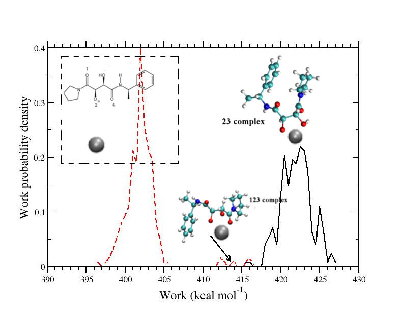
Figure 1: Forward (solid, black) and reverse (dashed, red) work distribution in the Zn(MBET306)^-1 complex in water calculated using fast switching NE simulations.

In the Figure 1, I report, as an illustrative example, the forward and reverse work distribution in a real unrestrained fast switching NE-simulations, that is the annihilation/growth of the Zinc(II) cation in the Zinc(II)-MBET306⁺ complex in explicit water in standard condition in a cubic MD box of volume $V_{\rm box}\simeq 15000~{}\AA^{3}$. The distribution were obtained using 256 annihilation/growth runs each lasting 90 ps. Further details on the simulations are given in Ref.Sandberg et al. (2015) On the right (solid black line), we have the annihilation work distribution $P(W_{1\rightarrow 0})$ of the principal bound state of the Zn-MBET306⁺ bound species. On the left (dashed red line), I report the reverse distribution $P(-W_{0\rightarrow 1})$ corresponding to the growth of the Zinc(II) cation from a random position in the MD box in presence of the MBET306^-1 receptor, where the most likely final NE-state corresponds to an unbound Zinc(II) in the bulk solvent. The small features of $P(-W_{0\rightarrow 1})$, at about 410:415 kcal mol^-1 with overall weight proportional to with $V_{\rm site}/V_{\rm box}$, corresponds to a few trajectories yielding a work that is related to the secondary poses of the Zn(II) on the MBET306^- anion.

The pattern shown in Figure 1 closely resembles that seen in systems where one direction of the $\tau$-NE experiment envisages the entrance in a funnel, like in the folding of a small poli-peptide.Procacci (2015) The entrance in the exclusion zone (that for the case of the Zn(MBET306)⁺ complex reported in Figure 1 corresponds roughly to the volume surrounding the central tartrate core of the molecule), via fast-growth from randomly sampled positions in a volume that is much larger than $V_{\rm site}$, is a far more dissipative process than the alchemically driven escape of the ligand from the binding site. Based on this analogy, we make the Ansatz that the forward decoupling work distribution $P(W_{1\rightarrow 0})$ for tightly bound ligand receptor system is made of essentially of one principal normal distribution relative to the starting stable pose of the ligand in the exclusion zone, $N(W,\mu,\sigma)$, and by a negligibly small volume-related work distribution $N(W,\mu_{\rm box},\sigma_{\rm box})$ due to sub-optimal poses or unbound states that could be detected in the reverse recoupling process:

$$P(W_{1\rightarrow 0}) = (1-c)N(W,\mu,\sigma)+cN(W,\mu_{\rm box},\sigma_{\rm box})$$ (17)

In Eq. 17 we have therefore that $c\ll 1$. With this regard, it is important to realize that, the second normal component depending on $\mu_{\rm box}$, while negligible in shaping the forward distribution, because of the Crooks theorem Eq. 11 gets exponentially amplified in the reverse process (see Eq. 15). We further assume, in Eq. 17, that $0<\mu_{\rm box}<\mu$ and $\sigma\simeq\sigma_{\rm box}$. The first assumption simply says that the non covalent complex exists, and hence one must do work to switch off the interaction with the environment and that this work must be larger than the mean work $\mu_{\rm box}$ done to switch off the interaction with the environment when the ligand may no longer be in the exclusion zone. The second simplifying assumption implies no loss of generalityProcacci (2015) and is based on the reasonable expectation that the mean dissipation, $\beta\sigma^{2}/2$, depends in essence on the particle density in the given thermodynamic conditions and that therefore $\sigma$ should be weakly dependent on the environment surrounding the ligand. Given the forward distribution Eq. 17, the Crooks theorem, Eq. 13, imposes that the reverse distribution,

$$P(-W_{0\rightarrow 1}) = d~{}N(W,\nu,\sigma)+(1-d)N(W,\nu_{\rm box},\sigma_{\rm box})$$ (18)

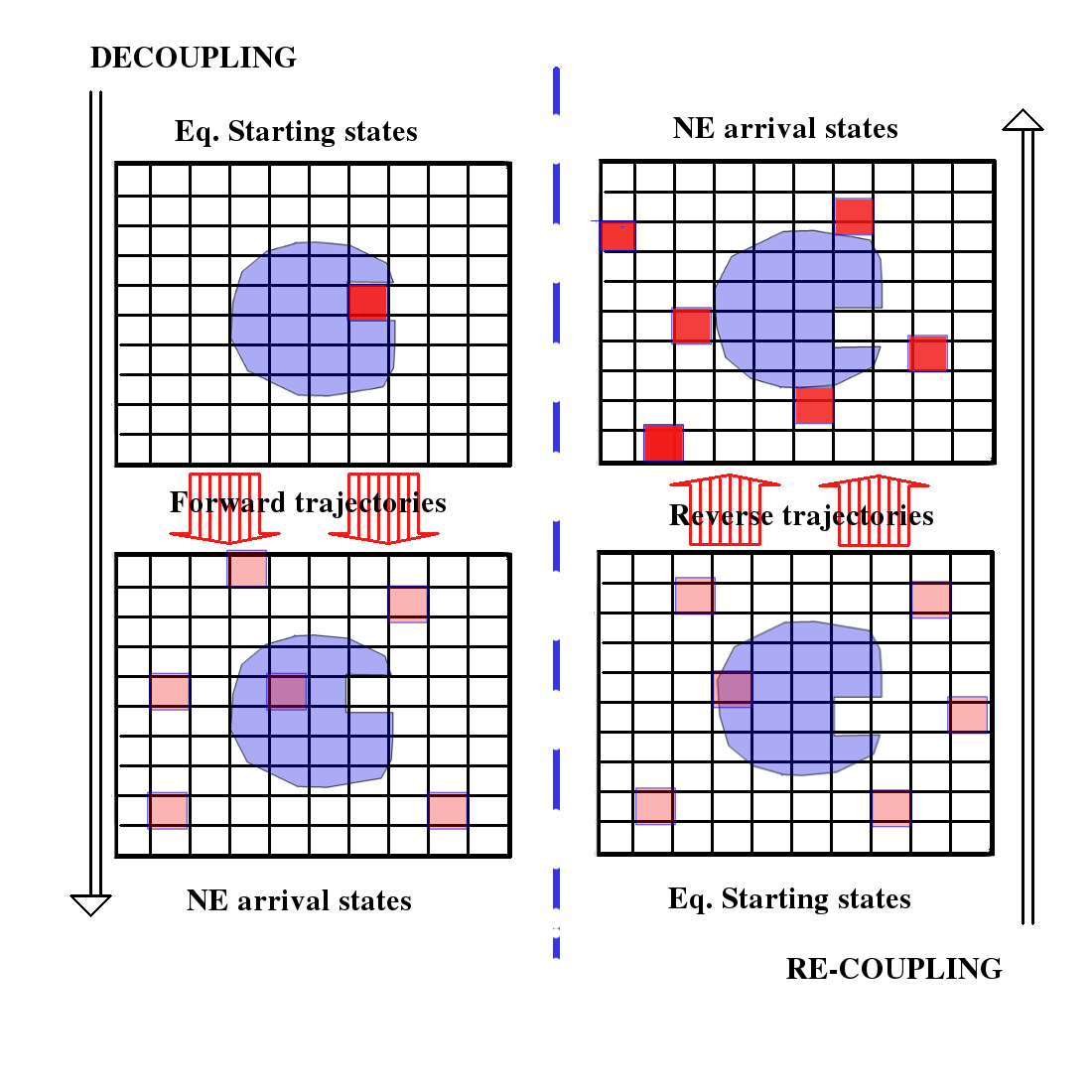
Figure 2: Forward/decoupling (left) and reverse/re-coupling (right) NE alchemical process in drugs receptor system. Six possible outcomes of NE trajectories are shown. The receptor is depicted in blue with the a square-shaped exclusion zone to allocate the ligand corresponding to a single box unit of the 2D-grid. The drug is red when is fully interacting with the environment and is light red when is in the decoupled state. In the forward process on the left, all the $N_{\tau}$ equilibrium starting configurations are in the bound state and the final states the ligand ends up in a random position in the MD box. In the reverse process, the decoupled ligand is initially randomly distributed in the box and ends in different unbound states or sub-optimal poses on the receptor. The probability to end up in the correct bound state is given by the volume of the exclusion zone divided by the total volume of the MD box, i.e. to $1/N_{\rm grid}$.

is such that $\nu=\mu-\beta\sigma^{2}$ and $\nu_{\rm box}=\mu_{\rm box}-\beta\sigma^{2}$ (See Eq. 14). The weight $d$ of the reverse Gaussian normal component with mean $\nu$ in Eq. 18 equals the probability of growing the ligand in the exclusion zone form a random position in the volume $V_{\rm box}$, i.e

$$d=V_{\rm site}/V_{\rm box}.$$ (19)

If $V_{\rm box}\gg V_{\rm site}$, as it occurs in the simulation practice, then $d$ is small and the principal component of the reverse process is $N(W,\nu_{\rm box},\sigma_{\rm box})$. The volume dependent free energy $\Delta G_{\rm RL}$ is found at the crossing point of the $\mu$-related forward and reverse Gaussian component:

$$\Delta G_{\rm RL} = \mu-\frac{1}{2}\beta\sigma^{2}+k_{B}T\ln\frac{d}{1-c}$$ (20)

$$\simeq \Delta G_{x}+k_{B}T\ln d$$

where in the last equation we have exploited the fact that $c\ll 1$ and we have defined $\Delta G_{x}=\mu-\frac{1}{2}\beta\sigma^{2}$. For Gaussian NE processes, the quantity $\mu-\frac{1}{2}\beta\sigma^{2}$ should be invariant with respect the duration time $\tau$ of the experiment, always yielding the minimum reversible work to do the transformation. As a matter of fact, if we make $V_{\rm box}$ larger, we need to set $\tau_{\rm box}$ larger but we clearly have no impact on the mean work $\mu$ done up to $\tau$. So $\Delta G_{x}$, unlike the crossing point $\Delta G_{\rm sim}$, does not depend on the box volume. Using Eq. 19 we finally find

$$\Delta G_{\rm RL} = \Delta G_{x}+k_{B}T\ln\frac{V_{\rm site}}{V_{\rm box}}$$ (21)

$$= \Delta G_{x}+k_{B}T\ln\frac{V_{site}}{V_{0}}-k_{B}T\ln\frac{V_{\rm box}}{V_{0}}$$ (22)

By subtracting on both side of Eq. 22 the volume independent solvation free energy of the ligand $\Delta G_{\rm L}$ and by using Eq. 16, we finally find that the standard dissociation free energy in NE alchemical transformation is given by

$$\Delta G_{0}=\Delta G_{x}-\Delta G_{\rm L}+k_{B}T\ln\frac{V_{site}}{V_{0}}$$ (23)

In deriving Eq. 23 from NE theory, DAM theory is somehow vindicated. The annihilation free energy of the complex in DAM may be thought as being derived from a high number of slow (ns time scale) quasi-equilibrium trajectories yielding a very sharp and normally distributed $\Delta G_{x}$ plus a shadow state that could be visible only if one does the reverse reaction, i.e. the switching on of the ligand in a random position of the MD box, in presence of the receptor. In the context of NE thermodynamics, the DAM free energy $\Delta G_{x}$ is indeed a system dependent quantity as conjectured in Ref. Fujitani et al. (2009); Jayachandran et al. (2006) that needs only to be shifted to match the SSC reference value by the $k_{B}T\ln\frac{V_{site}}{V_{0}}$. This correction for drug size ligand, is actually very small. Using value of 10 ų as the mean volume per atom in condensed phases in standard conditions, we may estimate $V_{\rm site}$ using the volume of the ligand itself, obtaining a SSC correction ranging from -0.7:0.1 kcal mol^-1.Jayachandran et al. (2006)

V Competitive poses and conformational sampling in non equilibrium simulations

We have seen that FS-DAM and DAM can be both embedded in the context of non equilibrium transformations. FS-DAM and DAM differ only in the speed of the NE process, fast in FS-DAM, very slow in DAM. In both cases the distribution $P(W_{1\rightarrow 0})$ for the annihilation of the ligand is normal with insignificant contamination by normal components of shadow states due to poses outside the exclusion zone or to unbound states. The distributions relative to these shadow states are exponentially amplified via Eq. 15 in a hypothetical (and unnecessary) reverse process where we grow the gas-phase ligand in a random position in the MD box and with random orientation with respect to the receptor, producing, when dealing with tight-binding ligand, a main normal component $N(W,\nu_{\rm box})$ with no overlap with the forward Gaussian component $N(W,\mu)$ as shown in the example reported in Figure 1.

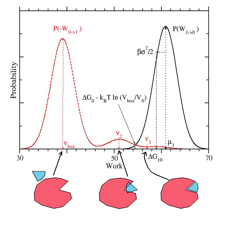
Figure 3: Schematic representation of the forward and reverse work distribution in the alchemical decoupling process for a ligand with one principal pose and with a secondary orientational pose (see text for details). Normal components related to unfavorable ligand-receptor free energy basins are exponentially amplified in a hypothetical reverse process (dashed, red line). Assuming that the volume of the exclusion zone is such that $V_{\rm site}\simeq V_{0}$, the example show a possible $P(W_{1\rightarrow 0}),~{}P(-W_{0\rightarrow 1})$ diagram for a ligand with a dissociation energy in the order of 20 $k_{B}T$.

We have also seen, in the preceding section that, given a spread of the work distribution of few kcal mol ^-1 for speeds of the decoupling process lasting in the order of 50:300 picoseconds, few hundreds of $\tau$-NE trajectories are sufficient for getting an accuracy within 0.5 kcal mol^-1 in the dissociation free energy.Sandberg et al. (2015) In the scheme reported in Figure 2 we have implicitly assumed that the bound state free energy is independent of the orientation of the ligand in the binding site. In reality, the ligand could be found in the exclusion zone with, e.g., several competing and mutually exclusive orientational poses (or free energy basins), with one of such poses being much more favorable than all the others (see Eq. 9). A minimum relative free energy difference such that ${\rm Min}_{i\neq 1}(\Delta G^{i}_{1})>3.72$ kcal mol^-1 translates in a probability ratio $P_{i}/P_{1}<1/512$ and is hence sufficient to exclude all the conformations due to the secondary poses $i=2..N_{p}$ from the pool of the few hundreds starting states of the bound complex randomly sampled out an equilibrium distribution. It follows that the apparent distribution due to the $N_{\tau}$ trajectories is again, in essence, normal, although is now made (in the limit $N_{\tau}\rightarrow\infty$ or for averages over infinite non overlapping bootstrap $N_{\tau}$ samples) of three components, namely that due to the principal pose, that due to the secondary poses in the exclusion zone with weight $c_{2}=e^{-\beta\Delta G^{2}_{1}}<\frac{1}{512}$ and the shadow state due to the sub-optimal poses on the receptor surface outside the exclusion zone or in the solvent with even smaller weight $c_{\rm box}\simeq e^{-\beta\Delta G_{0}}$:

$$P(W_{1\rightarrow 0}) = (1-c_{2}-c_{\rm box})N(W,\mu_{1},\sigma)+c_{2}N(W,\mu_{2},\sigma)+$$ (24)

$$+ c_{\rm box}N(W,\mu_{\rm box},\sigma).$$

where, for the sake of simplicity, we have assumed a pose independent spread/dissipation $\sigma$ for all $\tau$ lasting NE annihilation/growth processes. As already discussed, the Gaussian nature of the annihilation work distribution is somehow guaranteed by the speed (few tens of few hundreds of picoseconds) with which the alchemical decoupling is carried on allowing only marginal mixing between the underlying free energy basins at the intermediate NE $\lambda$ states. This is clearly at variance with reversible transformations, especially when implemented with $\lambda$-hopping schemes, that are introduced precisely to favor the canonical mixing all along the alchemical coordinate. It should also be noted that $\lambda$-hopping schemes, based on probabilistic criteria for the $\lambda$ dynamics, are either at convergence or they are incompatible with NE theory since they make the annihilation process not invertible. We have seen that the $\nu_{\rm box}$ related coefficient, $1-d$, in the reverse distribution of Eq. 18 gets exponentially amplified via the Crooks theorem-derived Eq. 15. By the same token, in a hypothetical reverse process, the normal components due to secondary poses in the exclusion zone are exponentially amplified via Eq. 15 so that the bound-stated related minor peak at $\nu$ integrating to $V_{\rm site}/V_{\rm box}$ (see Eq. 18 and Eq. 19) gets split in a left-most peak due to the manifold of secondary poses and to a smaller peak due to the principal pose whose height is proportional to the ratio $\xi(\Omega)/8\pi^{2}$ where $\xi(\Omega)$ is the fraction the domain $\{{\bf r},\Omega\}:I({\bf r},\Omega)=1$. On the overall, the Crooks theorem-related reverse distribution is of the form

$$P(-W_{0\rightarrow 1}) = d_{1}~{}N(W,\nu_{1},\sigma)+d_{2}N(W,\nu_{2},\sigma)+$$ (25)

$$+ (1-d_{1}-d_{2})N(W,\nu_{\rm box},\sigma).$$

with $d_{1}<d_{2}<(1-d_{1}-d_{2})$. In Figure 3 these concepts are schematized. The reverse distribution (dashed, red line) exhibits a principal left-most peak, $\nu_{\rm box}$, due to the sub-optimal poses off the binding site, an intermediate peak $\nu_{2}$ due a wrongly oriented poses in the binding site and a weak component due to the primary pose $\nu_{1}=\nu$ that is strongly overlapping with the forward apparently single component annihilation distribution. Assuming for the sake of simplicity and without loss of generality that $V_{\rm site}\simeq V_{0}$ such that $\Delta G_{x}\simeq\Delta G_{0}$, the crossing point of the forward and reverse distribution is again, as in Eq. 20, at the point $\Delta G_{0}+k_{B}T\ln d$ and again the free energy $\Delta G_{0}$ can be computed using the single Gaussian unbiased estimate of Eq. 12. In order to convey the concept, the weight of the components due to the bound states, $\nu_{1}$ and $\nu_{2}$ in the 3-G reverse distribution of Eq. 25 have been greatly exaggerated. Actually, the ratio $V_{\rm site}/V_{\rm box}$, i.e. the overall weight of the bound states in the unrestrained reverse distribution for real drug-receptor system is expected in the range $V_{\rm site}/V_{\rm box}$=0.01:0.001, implying that only few trajectories out of hundreds could produce a work corresponding to a bound state, exactly as observed in the growth of the Zinc(II) cation in presence of the MBET306^- anion (see Figure 1). Besides, the peak relative to the principal pose, $\nu_{1}$, is exponentially abated via Eq. 15 so that basically none out of few hundreds reverse NE trajectories is expected to yield a work (with inverted sign) falling near the forward distribution $P(W_{1\rightarrow 0})$. Based on the reverse process shown in Figure 1 for a simple atomic ligand, we conclude that a hypothetical reverse process in unrestrained NE DAM in real drug-receptor systems would systematically produce a forward and reverse distributions separated by a large gap, related to the dissociation energy itself, making bidirectional estimates such as Bennett acceptance ratio unreliable.Procacci (2015) The principal-pose assumption in the bound complex, leading to Eq. 9, constitutes the thermodynamic basis for molecular recognition. Most importantly, the existence of a pose with overwhelming Boltzmann weight in the complex implies a nearly Gaussian distribution in the $\tau$-NE decoupling of the ligand, allowing a reliable and unbiased estimate of the annihilation free energy $\Delta G_{\rm RL}$ to be obtained via the simple, unbiased Gaussian estimate Eq. 12. Such principal pose must of course be known from the start to be able to sample the equilibrium initial states at $\lambda=1$ in the corresponding free energy basin via standard molecular dynamics. Secondary poses can be checked in a similar manner, in a separate and independent NE experiment by using initial states all sampled in the corresponding secondary free energy basins. Again, if the NE simulations are so fast that only marginal mixing occurs among poses during the decoupling of the ligand, then the absolute dissociation free energy, $\Delta G_{i0}$ of the $i$-th secondary pose can also be determined using a simple Gaussian estimate, yielding as a trivial byproduct, the relative free energy difference $\Delta G_{1}^{i}=\Delta G_{i0}-\Delta G_{10}$, i.e the Boltzmann weight of the $i$-th pose relative to the principal pose, $\exp(-\beta(\Delta G_{i0}-\Delta G_{10}$). Such an approach has been used successfully in Ref. Sandberg et al. (2015) to derive the overall binding constant in water of the complex of the Zinc(II) with the MBET306^-1 anion, an inhibitor of the Tumor necrosis factor $\alpha$ converting enzyme. In that study, Sandberg et al. examined via NE unrestrained unidirectional simulations more than ten different poses of the cation on the tartaric moiety of MBET306^-.

VI Fast Switching calculation of solvation energies $\Delta G_{\rm L}$

In the complex, the preparation of the equilibrium starting states is an easy one. The ligand, by filling the exclusion zone of the receptor, inhibits its conformational motion and that of the protein residues delimiting the binding site, hence reducing the conformational entropy of the complex.

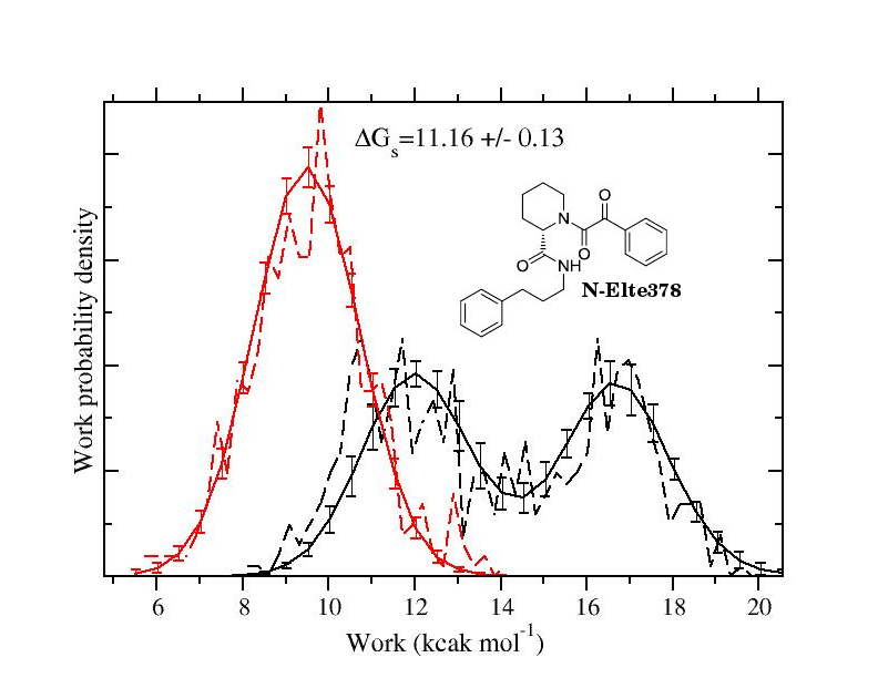
Figure 4: Fast switching forward (dashed black) and reverse (dashed red) work distributions obtained for N-Elte378 in water ($N_{\tau}=512$, $\tau$=270 ps. The free energy was evaluated using Eq. 13 assuming two normal components. Error bars reported on the fitted distributions (solid lines) were computed by bootstrapping samples of 256 works.

Once the $N_{\tau}$ NE independent trajectories from these states are launched, unlike in $\lambda$-hopping reversible DDM, we are no longer concerned with equilibrium sampling. Each $\lambda$-driven trajectory ends up irreversibly in the NE final decoupled state producing a mean work that depends chiefly on the enthalpy of the starting equilibrium state and not on the intermediate states that are rapidly crossed. FS-DAM, like DAM, needs also to annihilate the ligand in the bulk to get $\Delta G_{\rm L}$ and hence $\Delta G_{0}$ via Eq. 23. While the calculation of $\Delta G_{\rm L}$ is computationally far less demanding than the decoupling free energy of the bound state, the starting equilibrium states of the free ligand in bulk, especially when the ligand exhibits competing conformations of comparable free energies, should be prepared with the due care. I report as an illustrative example the case of the N-Elte378 [(2S)-1-(2-oxo-2-phenylacetyl)-N-(3-phenylpropyl) piperidine-2-carboxamide], a tight binding synthetic ligand of the immunophilin FKBP12.Martina et al. (2013). N-Elte378, a conformationally disordered molecule, can be characterized in water by a competition between extended and compact conformations (see Figure 7 of ref. Martina et al. (2013)), the latter being stabilized by persistent stacking interaction involving the two terminal phenyl moieties. The starting equilibrium configurations of N-Elte378 in water for the fast switching calculation of $\Delta G_{\rm L}$ in bulk are taken from a Hamiltonian Replica Exchange simulation with torsional tempering reported in Ref. Martina et al. (2013). Simulations details and methods can be found in Ref. Martina et al. (2013). The fast annihilation (forward) works were obtained running, in a single parallel run, 512 NE-trajectories lasting 270 ps. During the NE process, the solute is linearly discharged in the first 120 ps, followed by the switching off of 2/3 of the dispersive-repulsive interactions up to 150 ps. In the last 120 ps the residual Lennard-Jones interaction is finally switched off, using a soft-core regularization to avoid numerical instabilities near $\lambda=0$.Beutler et al. (1994) The fast growth (reverse) work from gas-phase N-Elte378 were collected with inverted time schedule using again 512 NE trajectories. The parallel computations were done using the fast switching alchemy version of the ORAC codeProcacci and Cardelli (2014); Marsili et al. (2010) in less than one wall-clock time hour. In Figure 4, I report the computed forward and reverse work distributions for N-Elte378 in water (dashed lines) along with the fitted distributions using Eq. 13 with two normal components (solid lines). Due to the complex conformational manifold, and because of the significant mixing between conformations during the 270 ps decoupling process, the annihilation work distribution in solvated N-Elte378 does not appear as a simple normal distribution, roughly reflecting the bi-modal structure observed in the probability distribution of the distance between the two terminal phenyl moieties (see Figure 7 of Ref. Martina et al. (2013)). Still, Eq. 13 explains very well the observed strikingly asymmetrical forward and reverse distributions, that were fitted assuming two normal components ($N=2$ in Eq. 13). The errors bars on the fitted distributions and on the hydration free energy are computed by block bootstrapping the collection of 512 work using 40 samples with 256 works. The bidirectional free energy computed using the Bennett acceptance ratio using the forward and reverse 512 works is computed at 11.02 $\pm$ 0.05 kcal mol^-1, comparing favorably with the estimate of 11.16 $\pm$ 0.16 kcal mol^-1 based on Eq. 13.

VII Conclusions and perspective

In this study I have revisited the theory of non covalent bonding in the evaluation of the binding free energies in drug-receptor systems from a non equilibrium perspective. I have shown that, in the context of the alchemical approach, the dissociation free energy of the complex can be effectively and accurately derived producing few hundreds of non equilibrium unrestrained trajectories starting from canonically sampled fully coupled bound states. The inherent Gaussian nature of the probability of doing a work $W$ at the end of the fast annihilation process allows to recover the decoupling free energy using a very robust unidirectional unbiased estimate. The fast switching double annihilation estimate (FS-DAM) is based on the assumption that the forward annihilation and the hypothetical reverse growth work distributions of the ligand in the complex and in the bulk are given by a mixture of normal distributions with weights regulated by the Crooks theorem. The standard state correction, related to the volume of the exclusion zone in the receptor, arises naturally in non equilibrium alchemical transformations with no need for restraining the motion of the ligand in the bound state. Non equilibrium unrestricted alchemical transformations eliminate altogether the necessity for canonical sampling at intermediate $\lambda$ states that constitutes the major stumbling block in the reversible alchemical approach. In this regard, one of the most critical aspects in reversible alchemical simulations, intimately related to the sampling issue, is the need of minimizing the overall statistical uncertainty of the free energy evaluation with respect to the alchemical protocol, that is, of equalizing the contribution to the uncertainty across every point along the alchemical path. In FS-DAM, equilibrium sampling is required at one single point along the alchemical path, at the fully coupled Hamiltonian. As a consequence, the accuracy of FS-DAM free energies depends in a predictable way on the resolution of the resulting work distribution, i.e. on the ratio of the spread of the work distribution and on the number of NE independent trajectories. The Crooks theorem-based estimate of the FS-DAM free energies relies on the determination of the first two cumulant of a normal distribution, whose variance is subject to the ancillary $t$-statistics and is proportional to $\sigma(\tau)/(N_{\tau})^{1/2}$ and $\sigma^{2}(\tau)/(N_{\tau})^{1/2}$, where $\sigma(\tau)$ is the $\tau$-dependent spread of the distribution. Reducing the number of NE trajectories by a factor of $G$ amplifies the error on $\mu$ and $\sigma^{2}$ only by $G^{1/2}$ making FS-DAM estimates extremely robust and reliable even with a very small number of sampling trajectories.Procacci (2015)

As the NE-trajectories can be run independently, the FS-DAM approach can be straightforwardly and efficiently implemented on massively parallel platforms providing an effective tool for virtual screening in the drug discovery process. In the applicative companion paperNerattini et al. (2016) of the present theoretical contribution, we apply the FS-DAM technology to a challenging drug-receptor system, the FKBP12 protein associated to the FK506 related ligands, comparing performances and accuracy to the standard equilibrium approach. In that study Nerattini et al. (2016) we show that FS-DAM satisfactorily reproduces the experimental dissociation free energies of several FK506-related bulky ligands towards the native FKBP12 enzyme in a single massively parallel run in matter of few wall time clock hours on a High Performance Computing facility. FS-DAM is finally used to predict the dissociation constants for the same ligands towards the FKBP12 mutant Ile56Asp. The effect of such mutation on the binding affinity of FK506-related ligands is relevant for assessing the thermodynamic forces regulating molecular recognition in FKBP12 inhibition. Moreover, the binding affinities of FK506-related ligands for the Ile56Asp FKBP12 mutant are, to our knowledge, not yet available, exposing our FS-DAM predictions to experimental verification. Anticipating the results presented in Ref. Nerattini et al. (2016), we summarize in Table 2 performance and accuracy tests of the FS-DAM method compared to the standard equilibrium approaches for the evaluation of the dissociation constant of a drug-receptor pair in explicit solvent.

	$N_{\tau}$	$N_{\lambda}$	Simulation time	Mean error on
			(ns per ligand)	$\Delta G_{0}$ (kcal mol-1)
FS-DAM	512	n/a	218	0.3
FS-DAM	256	n/a	149	0.7
FS-DAM	128	n/a	115	1.5
FEPShirts (2005)	n/a	31	18000	1.5
FEPFujitani et al. (2005)	n/a	33	400	4.5
FEP/BARFujitani et al. (2009)	n/a	32	900	3.0
FEP-restraintWang et al. (2006)	n/a	25	250	1.5

Table 2: Performances of NE FS-DAM and equilibrium FEP. $N_{\tau}$ and $N_{\lambda}$ indicate the number of independent NE trajectories (applicable in FS-DAM only) and the number of $\lambda$ intermediate states (applicable in FEP only). All data refer to the FKBP12 receptorNerattini et al. (2016) on per ligand basis.

These results are fully detailed in Ref. Nerattini et al. (2016) and show that FS-DAM outperforms FEP approaches,Shirts (2005); Fujitani et al. (2005, 2009) both in terms of precision/reliability and of CPU time. The efficiency, simplicity and inherent parallel nature of FS-DAM, project the methodology as a possible effective tool for a second generation High Throughput Virtual Screening in drug discovery and design.

VIII Acknowledgements

The computing resources and the related technical support used for this work have been provided by CRESCO/ENEAGRID High Performance Computing infrastructure and its staff.Ponti et al. (2014) CRESCO/ENEAGRID High Performance Computing infrastructure is funded by ENEA, the Italian National Agency for New Technologies, Energy and Sustainable Economic Development and by Italian and European research programmes, see http://www.cresco.enea.it/english for information

References

- Munos (2009) B. Munos, Nat Rev Drug Discov, 2009, 8, 959–968.
- Scannell et al. (2012) J. W. Scannell, A. Blanckley, H. Boldon and B. Warrington, Nat Rev Drug Discov, 2012, 11, 191–200.
- (3) See for example the Pharmaceutical Research and Manufacturers of America (PhRMA) Fact Sheet ”Drug Discovery and Development. Understanding the R&D process” available at the internet address http://www.phrma.org/ (accessed 01/05/2015).
- Lavecchia and Di-Giovanni (2013) A. Lavecchia and C. Di-Giovanni, Curr. Med. Chem., 2013, 20, 2839–2860.
- Marechal et al. (2011) Chemogenomics and Chemical Genetics.A User’s Introduction for Biologists, Chemists and Informaticians, ed. E. Marechal, S. Roy and L. Lafanechere, Springer-Verlag Berlin Heidelberg, 2011.
- Chodera et al. (2011) J. Chodera, D. Mobley, M. Shirts, R. Dixon, K.Branson and V. Pande, Curr. Opin Struct. Biol, 2011, 21, 150–160.
- Deng et al. (2015) N. Deng, S. Forli, P. He, A. Perryman, L. Wickstrom, R. S. K. Vijayan, T. Tiefenbrunn, D. Stout, E. Gallicchio, A. J. Olson and R. M. Levy, The Journal of Physical Chemistry B, 2015, 119, 976–988.
- Gilson et al. (1997) M. K. Gilson, J. A. Given, B. L. Bush and J. A. McCammon, Biophys. J., 1997, 72, 1047–1069.
- Woo and Roux (2005) H.-J. Woo and B. Roux, Proc. Natnl. Acad. Sci. USA, 2005, 102, 6825–6830.
- Colizzi et al. (2010) F. Colizzi, R. Perozzo, L. Scapozza, M. Recanatini and A. Cavalli, J. Am. Chem. Soc., 2010, 132, 7361–7371.
- Laio and Parrinello (2002) A. Laio and M. Parrinello, Proc. Natl. Acad. Sci. USA, 2002, 99, 12562–12566.
- Fidelak et al. (2010) J. Fidelak, J. Juraszek, D. Branduardi, M. Bianciotto and F. L. Gervasio, J. Phys. Chem. B, 2010, 114, 9516–9524.
- Biarnes et al. (2011) X. Biarnes, S. Bongarzone, A. Vargiu, P. Carloni and P. Ruggerone, Journal of Computer-Aided Molecular Design, 2011, 25, 395–402.
- Gallicchio et al. (2010) E. Gallicchio, M. Lapelosa and R. M. Levy, J. Chem. Theory Comput., 2010, 6, 2961–2977.
- Fasnacht et al. (2004) M. Fasnacht, R. H. Swendsen and J. M. Rosenberg, Phys. Rev. E, 2004, 69, 056704.
- Procacci et al. (2014) P. Procacci, M. Bizzarri and S. Marsili, J Chem. Theory Comp., 2014, 10, 439–450.
- Gumbart et al. (2013) J. C. Gumbart, B. Roux and C. Chipot, J. Chem. Theory Comput., 2013, 9, 974–802.
- Jorgensen and Ravimohan (1985) W. Jorgensen and C. Ravimohan, J. Chem. Phys., 1985, 83, 3050–3054.
- Shirts et al. (2007) M. Shirts, D. Mobley and J. Chodera, Annu. Rep. Comp Chem., 2007, 3, 41–59.
- Jorgensen and Thomas (2008) W. Jorgensen and L. Thomas, J. Chem. Theory Comput., 2008, 4, 869–876.
- Deng and Roux (2009) Y. Deng and B. Roux, J. Phys. Chem. B, 2009, 113, 2234–2246.
- Gallicchio and Levy (2011) E. Gallicchio and R. M. Levy, Current Opinion in Structural Biology, 2011, 21, 161 – 166.
- Hansen and van Gunsteren (2014) N. Hansen and W. F. van Gunsteren, Journal of Chemical Theory and Computation, 2014, 10, 2632–2647.
- Wang et al. (2015) L. Wang, Y. Wu, Y. Deng, B. Kim, L. Pierce, G. Krilov, D. Lupyan, S. Robinson, M. K. Dahlgren, J. Greenwood, D. L. Romero, C. Masse, J. L. Knight, T. Steinbrecher, T. Beuming, W. Damm, E. Harder, W. Sherman, M. Brewer, R. Wester, M. Murcko, L. Frye, R. Farid, T. Lin, D. L. Mobley, W. L. Jorgensen, B. J. Berne, R. A. Friesner and R. Abel, Journal of the American Chemical Society, 2015, 137, 2695–2703.
- Phillips et al. (2005) J. C. Phillips, R. Braun, W. Wang, J. Gumbart, E. Tajkhorshid, E. Villa, C. Chipot, L. Skeel and K. Schulten, J. Comput. Chem., 2005, 26, 1781–1802.
- Kirkwood (1935) J. G. Kirkwood, J. Chem. Phys., 1935, 3, 300–313.
- Zwanzig (1954) R. W. Zwanzig, J. Chem. Phys., 1954, 22, 1420–1426.
- Bennett (1976) C. H. Bennett, J. Comp. Phys., 1976, 22, 245–268.
- Shirts et al. (2003) M. R. Shirts, E. Bair, G. Hooker and V. S. Pande, Phys. Rev. Lett., 2003, 91, 140601.
- Procacci (2013) P. Procacci, J. Chem. Phys., 2013, 139, 124105.
- General (2010) I. J. General, Journal of Chemical Theory and Computation, 2010, 6, 2520–2524.
- Procacci (2015) P. Procacci, The Journal of Chemical Physics, 2015, 142, 154117.
- Kaus and McCammon (2015) J. W. Kaus and J. A. McCammon, J. Phys. Chem. B, 2015, 119, 6190–6197.
- Fujitani et al. (2009) H. Fujitani, Y. Tanida and A. Matsuura, Phys. Rev. E, 2009, 79, 021914.
- Yamashita et al. (2015) T. Yamashita, A. Ueda, T. Mitsui, A. Tomonaga, S. Matsumoto, T. Kodama and H. Fujitani, Chemical and Pharmaceutical Bulletin, 2015, 63, 147–155.
- Naden and Shirts (2015) L. N. Naden and M. R. Shirts, Journal of Chemical Theory and Computation, 2015, 11, 2536–2549.
- Jayachandran et al. (2006) G. Jayachandran, M. R. Shirts, S. Park and V. S. Pande, The Journal of Chemical Physics, 2006, 125, 084901.
- Sandberg et al. (2015) R. B. Sandberg, M. Banchelli, C. Guardiani, S. Menichetti, G. Caminati and P. Procacci, Journal of Chemical Theory and Computation, 2015, 11, 423–435.
- Procacci and Cardelli (2014) P. Procacci and C. Cardelli, J. Chem. Theory Comput., 2014, 10, 2813–2823.
- Crooks (1998) G. E. Crooks, J. Stat. Phys., 1998, 90, 1481–1487.
- Mihailescu and Gilson (2004) M. Mihailescu and M. K. Gilson, Biophysical Journal, 2004, 87, 23 – 36.
- Luo and Sharp (2002) H. Luo and K. Sharp, Proc. Natnl. Acad. Sci. USA, 2002, 99, 10399–10404.
- Zhou and Gilson (2009) H.-X. Zhou and M. K. Gilson, Chem. Rev., 2009, 109, 4092–4107.
- Baron et al. (2010) R. Baron, P. Setny and J. A. McCammon, J. Am. Chem. Soc., 2010, 132, 12091–12097.
- Boresch et al. (2003) S. Boresch, F. Tettinger, M. Leitgeb and M. Karplus, The Journal of Physical Chemistry B, 2003, 107, 9535–9551.
- Beutler et al. (1994) T. Beutler, A. Mark, R. van Schaik, P. Gerber and W. van Gunsteren, Chem. Phys. Lett., 1994, 222, 5229–539.
- Buelens and Grubmüller (2012) F. Buelens and H. Grubmüller, Journal of Computational Chemistry, 2012, 33, 25–33.
- Hermans and Wang (1997) J. Hermans and L. Wang, Journal of the American Chemical Society, 1997, 119, 2707–2714.
- Pohorille et al. (2010) A. Pohorille, C. Jarzynski and C. Chipot, The Journal of Physical Chemistry B, 2010, 114, 10235–10253.
- Chelli (2010) R. Chelli, J. Chem. Theory Comput., 2010, 6, 1935–1950.
- Cumming et al. (2012) J. N. Cumming, E. M. Smith, L. Wang, J. Misiaszek, J. Durkin, J. Pan, U. Iserloh, Y. Wu, Z. Zhu, C. Strickland, J. Voigt, X. Chen, M. E. Kennedy, R. Kuvelkar, L. A. Hyde, K. Cox, L. Favreau, M. F. Czarniecki, W. J. Greenlee, B. A. McKittrick, E. M. Parker and A. W. Stamford, Bioorg. Med. Chem. Letters, 2012, 22, 2444 – 2449.
- Procacci et al. (2006) P. Procacci, S. Marsili, A. Barducci, G. F. Signorini and R. Chelli, J. Chem. Phys., 2006, 125, 164101.
- Jarzynski (1997) C. Jarzynski, Phys. Rev. Lett., 1997, 78, 2690–2693.
- Hummer (2001) G. Hummer, J. Chem. Phys., 2001, 114, 7330–7337.
- Gore et al. (2003) J. Gore, F. Ritort and C. Bustamante, Proc. Natnl. Acad. Sci., 2003, 100, 12564–12569.
- Park and Schulten (2004) S. Park and K. Schulten, J. Chem. Phys., 2004, 120, 5946–5961.
- Shirts and Pande (2005) M. R. Shirts and V. S. Pande, J. Chem. Phys., 2005, 122, 144107.
- Oberhofer et al. (2005) H. Oberhofer, C. Dellago and P. L. Geissler, The Journal of Physical Chemistry B, 2005, 109, 6902–6915.
- Goette and Grubmüller (2009) M. Goette and H. Grubmüller, Journal of Computational Chemistry, 2009, 30, 447–456.
- Gapsys et al. (2015) V. Gapsys, S. Michielssens, J. Peters, B. de Groot and H. Leonov, Molecular Modeling of Proteins, Springer New York, 2015, vol. 1215, pp. 173–209.
- Feng and Crooks (2008) E. H. Feng and G. E. Crooks, Phys. Rev. Lett., 2008, 101, 090602.
- Procacci and Marsili (2010) P. Procacci and S. Marsili, Chem. Phys., 2010, 375, 8–15.
- Gapsys et al. (2012) V. Gapsys, D. Seeliger and B. de Groot, J. Chem. Teor. Comp., 2012, 8, 2373–2382.
- Marcinkiewicz (1939) J. Marcinkiewicz, Mathematische Zeitschrift, 1939, 44, 612–618.
- Krishnamoorthy (2006) K. Krishnamoorthy, Handbook of Statistical Distributions with Applications, Chapman and Hall/CRC, London (UK), 2006.
- Martina et al. (2013) M. R. Martina, E. Tenori, M. Bizzarri, S. Menichetti, G. Caminati and P. Procacci, J. Med. Chem., 2013, 56, 1041–1051.
- Marsili et al. (2010) S. Marsili, G. F. Signorini, R. Chelli, M. Marchi and P. Procacci, J. Comp. Chem., 2010, 31, 1106–1116.
- Nerattini et al. (2016) F. Nerattini, R. Chelli and P. Procacci, Phys. Chem. Chem. Phys., 2016, DOI: 10.1039/C5CP05521K.
- Shirts (2005) M. R. Shirts, PhD thesis, Stanford University CA, Stanford, California 94305, 2005.
- Fujitani et al. (2005) H. Fujitani, Y. Tanida, M. Ito, G. Jayachandran, C. D. Snow, M. R. Shirts, E. J. Sorin and V. S. Pande, The Journal of Chemical Physics, 2005, 123, 084108.
- Wang et al. (2006) J. Wang, Y. Deng, B. and Roux, Biophys. J., 2006, 91, 2798–2814.
- Ponti et al. (2014) G. Ponti, F. Palombi, D. Abate, F. Ambrosino, G. Aprea, T. Bastianelli, F. Beone, R. Bertini, G. Bracco, M. Caporicci, B. Calosso, M. Chinnici, A. Colavincenzo, A. Cucurullo, P. Dangelo, M. De Rosa, P. De Michele, A. Funel, G. Furini, D. Giammattei, S. Giusepponi, R. Guadagni, G. Guarnieri, A. Italiano, S. Magagnino, A. Mariano, G. Mencuccini, C. Mercuri, S. Migliori, P. Ornelli, S. Pecoraro, A. Perozziello, S. Pierattini, S. Podda, F. Poggi, A. Quintiliani, A. Rocchi, C. Scio, F. Simoni and A. Vita, Proceeding of the International Conference on High Performance Computing & Simulation, Institute of Electrical and Electronics Engineers ( IEEE ), 2014, pp. 1030–1033.