Interpolation across a muffin-tin interstitial using localized linear combinations of spherical waves

Yoshiro Nohara Current address: ASMS Co., Ltd., 1-7-11 Higashi-gotanda Shinagawa-ku, Tokyo 141-0022, Japan    O. K. Andersen Max Planck Institute for Solid State Research, Heisenbergstrasse 1, D-70569, Stuttgart, Germany
Abstract

A method for 3D interpolation between hard spheres is described. The function to be interpolated could be the charge density between atoms in condensed matter. Its electrostatic potential is found analytically, and so are various integrals. Periodicity is not required. The interpolation functions are localized structure-adapted linear combinations of spherical waves, socalled unitary spherical waves (USWs), $\psi_{RL}\left(\varepsilon,\mathbf{r}\right),$ centered at the spheres, $R,$ where they have cubic-harmonic character, $L.$ Input to the interpolation are the coefficients in the cubic-harmonic expansions of the target function at and slightly outside the spheres; specifically, the values and the 3 first radial derivatives labelled by $d=0$ (value), and 1-3 (derivatives). To fit this, we use USWs with 4 negative energies, $\varepsilon=\epsilon_{1},\epsilon_{2},\epsilon_{3}$ and $\epsilon_{4}.$ Each interpolation function, $\varrho_{dRL}\left(\mathbf{r}\right),$ is actually a linear combination of these 4 sets of USWs with the following properties: (1) It is centered at a specific sphere where it has a specific cubic-harmonic character and radial derivative. (2) Its value and first 3 radial derivatives vanish at all other spheres and for all other cubic-harmonic characters, and is therefore highly localized, essentially inside its Voronoi cell. Value-and-derivative (v&d) functions were originally introduced and used by Methfessel [Phys. Rev. B 38, 1537 (1988)], but only for the first radial derivative. Explicit expressions are given for the v&d functions and their Coulomb potentials in terms of the USWs at the 4 energies, plus $\epsilon_{0}\equiv 0$ for the potentials. The coefficients, as well as integrals over the interstitial such as the electrostatic energy, are given entirely in terms of the structure matrix, $S_{RL,R^{\prime}L^{\prime}}\left(\epsilon_{n}\right)$, describing the slopes of the USWs at the 5 energies and their expansions in Hankel functions. For open structures, additional constraints are installed to pinpoint the interpolated function deep in the interstitial. The strong localization of the v&d functions makes the method uniquely suited for complicated structures. Use of point- and space-group symmetries can significantly reduce matrix sizes and the number of v&d functions. As simple examples, we consider a constant density and the valence-electron densities in zinc-blende structured Si, ZnSe, and CuBr.

pacs:
02.30.-f, 71.15.-m, 71.15.Dx
preprint:

I Introduction

An often-met problem in computational physics, chemistry, and biology, and a key one in electronic density-functional calculations, is to express a smooth, global function, $\rho\left(\mathbf{r}\right),$ say the charge density, in the region between the atoms in a form suitable for finding its electrostatic potential, $V\left(\mathbf{r}\right),$ and for evaluating integrals such as an electrostatic energy $\int\rho\left(\mathbf{r}\right)V\left(\mathbf{r}\right)d^{3}r.$

It has been found useful to expand

$$\rho\left(\mathbf{r}\right)=\sum_{mn}\psi_{m}\left(\epsilon_{n},\mathbf{r}\right)c_{mn},$$

in solutions of the wave equation,

$$\left(\Delta+\varepsilon\right)\psi\left(\varepsilon,\mathbf{r}\right)=0,$$ (1)

because then, the solution of Poisson’s equation:

$$-\Delta V\left(\mathbf{r}\right)=8\pi\rho\left(\mathbf{r}\right)$$ (2)

(in atomic Ry units), is simply:

$$V\left(\mathbf{r}\right)=8\pi\left[\psi\left(0,\mathbf{r}\right)+\sum_{nm}\psi_{m}\left(\epsilon_{n},\mathbf{r}\right)c_{mn}/\epsilon_{n}\right].$$ (3)

The expansion functions, $\psi_{m}\left(\epsilon_{n},\mathbf{r}\right),$ need only be defined in the region of interest, while the particular solution, $\psi\left(0,\mathbf{r}\right),$ of the Laplace equation extends in all space.

A common choice of expansion functions is wave-equation solutions with transform according to an irreducible representation $\left(\mathbf{k}\right)$ of a crystal or supercell, i.e. plane waves, $e^{i\left(\mathbf{k+G}_{n}\right)\cdot\mathbf{r}},$ with $\left|\mathbf{k+G}_{n}\right|^{2}=\varepsilon\geq 0$ and $\mathbf{G}_{n}$ running over the vectors of the reciprocal lattice. For expanding a periodic function like the charge density, $\mathbf{k=0.}$ The plane-wave set is complete and orthonormal in the primitive cell, but is overcomplete and non-orthogonal in the interstitial, say between muffin-tin (MT) spheres surrounding the atoms and voids. Electronic-structure methods give the charge density as the sum of products of the electronic basis functions, and using plane waves for the latter, yields also the charge density as a sum of plane waves: $\sum e^{i\left(\mathbf{G}_{m}-\mathbf{G}_{n}\right)\cdot\mathbf{r}}c_{m}c_{n}^{\ast}$. With pseudopotential methods, this density is a smooth part of the true density and extends in all space, whereas with augmented plane-wave methods, it is the true density in the MT interstitial Martin ; 12MartinandTerakuras . Even in cases where the electronic basis functions are not plane waves, plane-wave expansion of the charge density is often used. With a small basis set of MT orbitals, for instance, a smooth part of the orbitals is either Fourier transformed and then multiplied together 85Weyrich ; 96Savrasov ; 00Wills , or multiplied together directly on a mesh and then Fourier transformed 00Methfessel ; 10Kotani .

In this paper, we shall not expand in plane waves because they are extended, but in MT-centered, decaying spherical waves, $h_{l}^{\left(1\right)}\left(\kappa r_{R}\right)Y_{L}\left(\mathbf{\hat{r}}_{R}\right),$ the natural choice for dealing with local point symmetries. Here and in the following, $r_{R}\equiv\left|\mathbf{r-R}\right|,$ $\mathbf{\hat{r}}_{R}\equiv\widehat{\mathbf{r-R}},$ $L\equiv lm,$ and $\kappa^{2}=\varepsilon\lesssim 0.$ Actually, we shall combine linearly the $RL$-set of spherical waves for a given energy and structure, as specified by its centers, $\mathbf{R,}$ and radii, $a_{R},$ into a set of even more localized, structure-adapted unitary spherical waves (USWs) 94Trieste , each of which is a cubic harmonic, $Y_{L}\left(\mathbf{\hat{r}}_{R}\right),$ on the own sphere and vanishes on all other spheres. Because of this requirement, the spheres cannot overlap. Moreover, the USWs are defined to vanish inside all spheres, which we shall therefore call hard- rather than MT spheres hardvsMT . A set of USWs is thus a set of localized, structure-adapted spherical waves with a given energy. Localization is essential if the computational effort is to increase merely proportional to the size of the system (or the number of inequivalent sites) 12orderN . The USW set, $\psi_{RL}\left(\varepsilon,\mathbf{r}\right),$ is specified by a structure- or slope matrix whose element, $S_{RL,R^{\prime}L^{\prime}}\left(\varepsilon\right),$ equals the radial derivative (slope) of the $R^{\prime}L^{\prime}$-projection of $\psi_{RL}\left(\varepsilon,\mathbf{r}\right)$, and also gives the coefficient to $h_{l^{\prime}}^{\left(1\right)}\left(\kappa r_{R^{\prime}}\right)Y_{L^{\prime}}\left(\mathbf{\hat{r}}_{R^{\prime}}\right)$ in the expansion of $\psi_{RL}\left(\varepsilon,\mathbf{r}\right)$.

When $\rho\left(\mathbf{r}\right)$ is better known – or simpler to evaluate – near the surfaces of the spheres than throughout the topologically complicated interstitial, it is advantageous to interpolate $\rho\left(\mathbf{r}\right)$ across the interstitial rather than to project it onto the interstitial. This is the case for the electronic density: Near the surface of any sphere surrounding an atom, this density is essentially the sum of products of occupied atomic orbitals and therefore has a cubic-harmonic expansion with $l_{\max}$ about twice the highest $l$ of an occupied atomic orbital. Near each sphere, one can therefore easily project $\rho\left(\mathbf{r}\right)$ onto cubic harmonics obtaining the radial functions, $\mathcal{\hat{P}}_{RL}\left(r\right)\rho\left(\mathbf{r}\right),$ and then search an expansion:

$$\rho\left(\mathbf{r}\right)=\sum_{n=1}^{d_{\max}+1}\sum_{RL}\,\psi_{RL}\left(\epsilon_{n},\mathbf{r}\right)c_{nRL},$$ (4)

in USWs with $d_{\max}+1$ different energies, which fits the values and first $d_{\max}$ radial derivatives at $a_{R}$ for all $RL.$ It is obvious that if we fit only values $\left(d_{\max}\mathrm{=}0\right),$ the unitary property of, $\psi_{RL}\left(\epsilon_{1},\mathbf{r}\right),$ leads to the simple result: $c_{0RL}=\mathcal{\hat{P}}_{RL}\left(a_{R}\right)\rho\left(\mathbf{r}\right).$ In order to fit also slopes $\left(d_{\max}\mathrm{=}1\right)$, we must solve $N_{R}N_{L}$ linear equations where $N_{R}$ the number of sites within the range of a USW and $N_{L}$ is the number of $L$ values. In case we need to interpolate the charge density many times for a given structure, as is the case in charge-selfconsistent electronic-structure calculations, we would invert the corresponding matrix for the linear equations once and for all. This matrix is the 1st energy-divided difference,

$$\frac{S\left(\epsilon_{1}\right)-S\left(\epsilon_{2}\right)}{\epsilon_{1}-\epsilon_{2}}\equiv S_{12},$$ (5)

of the slope matrix 94Trieste . In fact, $aS_{12}$ equals the integral $\left\langle\psi\left(\epsilon_{1}\right)\mid\psi\left(\epsilon_{2}\right)\right\rangle$ over the interstitial.

For general $d_{\max},$ the dimension of the matrix to be inverted would be $d_{\max}+1$ times as large. Considering the fact that changing the energy or the structure requires another inversion, this could be computationally demanding. In the present paper, we shall therefore derive explicit expressions involving merely the first $d_{\max}+1$ energy-divided differences of the slope matrix. This is achieved by exploiting the radial wave equation,

$$\left[r\psi_{l}\left(\varepsilon,r\right)\right]^{\prime\prime}=-\left[\varepsilon-l\left(l+1\right)/r^{2}\right]r\psi_{l}\left(\varepsilon,r\right),$$ (6)

with the two unitary boundary conditions: $r\psi_{l}\left(\varepsilon,r\right)|_{a}=1$ or $0.$ The simplest way to think about this approach is that for a given structure and symmetry, but independently of the function to be interpolated, we find those linear combinations, $\varrho_{dRL}\left(\mathbf{r}\right),$ of the USW sets for the energies $\epsilon_{1},\,\epsilon_{2},\,..,\,\epsilon_{d_{\max}}$ which have the ”super-unitary” property that the $d^{\prime}$th radial derivative, $\left[r\mathcal{\hat{P}}_{R^{\prime}L^{\prime}}\left(r\right)\varrho_{dRL}\left(\mathbf{r}\right)\right]^{\left(d^{\prime}\right)}$ at $a_{R^{\prime}},$ for all $R^{\prime},L^{\prime}$, and $d^{\prime}=0,...,d_{\max},$ vanish, except the own derivative $\left(d\right)$ of the own cubic-harmonics projection $\left(L\right)$ at the own sphere $\left(R\right)$. In terms of these value-and-derivative (v&d) functions, which are even more localized than the USWs, the density interpolated from its radial derivatives,

$$\mathcal{R}_{RL}^{\left(d\right)}\left(a_{R}\right)\equiv\left[r\mathcal{\hat{P}}_{RL}\left(r\right)\rho\left(\mathbf{r}\right)\right]_{a_{R}}^{\left(d\right)},$$ (7)

at the spheres is then:

$$\rho\left(\mathbf{r}\right)=\sum_{d=0}^{d_{\max}}\sum_{RL}\varrho_{dRL}\left(\mathbf{r}\right)\mathcal{R}_{RL}^{\left(d\right)}\left(a_{R}\right).$$ (8)

The v&d functions are localized essentially inside the Voronoi (Wigner-Seitz) cells and the expansion (8) is therefore similar to, but more general and efficient, than the one-center, cubic-harmonic expansion of the cell-truncated density 73Mol used in KKR 91KKRcell and LMTO00Kollar Green-function methods to treat molecules, crystals, impurities, random alloys, amorphous systems, surfaces, interfaces, etc., when going beyond the atomic-spheres approximation (ASA) 73Simple ; 75PRB ; 80Segall ; 83imp ; 84Skriver ; LamG ; Green ; Schilf ; Pessoa ; Nowak ; Bose ; Vargas ; Mook ; Abrikosov ; Ruban ; Turek ; Weinberger ; Stuttgart .

For each v&d function, $\varrho_{dRL}\left(\mathbf{r}\right),$ we can solve Poisson’s equation (2) and find the localized potential, $\varphi_{dRL}^{loc}\left(\mathbf{r}\right),$ and the multipoles which have been subtracted in order to make it localized. This potential and its multipole moments are expressed in terms of energy-divided differences 00DivDif of the USWs and the slope matrix over the energy mesh, $\epsilon_{0},\,\epsilon_{1},...,\,\epsilon_{d_{\max}+1},$ to which the energy $\epsilon_{0}\equiv 0$ has been added. The latter takes care of the particular solution in eq. (3) which picks the localized part of the potential. In terms of these potentials from the v&d charge densities, the localized Coulomb potential from $\rho\left(\mathbf{r}\right)$ is then:

$$V^{loc}\left(\mathbf{r}\right)=\sum_{d=0}^{d_{\max}}\sum_{RL}\varphi_{dRL}^{loc}\left(\mathbf{r}\right)\mathcal{R}_{RL}^{\left(d\right)}\left(a_{R}\right).$$ (9)

At the end of a calculation, the localizing multipoles are added to those from the remaining charge density in the system and the resulting Laplace potential is expanded in zero-energy USWs, $\psi_{RL}\left(0,\mathbf{r}\right).$

With the charge density and the Coulomb potential in the interstitial expressed in terms of USWs and their slope matrix, and with the integral of a product of USWs over the interstitial expressed in terms of the slope matrix (5), so is the electrostatic energy of the interstitial charge density. Also one-center cubic-harmonic expansions, such as:

$$\varphi_{dRL}^{loc}\left(\mathbf{r}\right)\approx\sum_{L^{\prime}}Y_{L^{\prime}}\left(\mathbf{\hat{r}}_{R^{\prime}}\right)\mathcal{\hat{P}}_{R^{\prime}L^{\prime}}\left(r\right)\varphi_{dRL}^{loc}\left(\mathbf{r}\right),$$ (10)

are given in terms of the slope matrix and two radial wave-equation solutions (6). The spherically symmetric averages $\left(L^{\prime}\mathrm{=}0\right)$ are for instance used to generate the potential in the overlapping MT approximation (OMTA) 98MRS ; 09OMTA which defines the 3rd generation LMTO 94Trieste ; 98MRS ; 00Rashmi and NMTO 00NMTO ; 00Odile ; 12Juelich ; 15FPNMTO basis sets.

The present paper reformulates and extends beyond 1st radial derivatives an approach proposed nearly 30 years ago by Methfessel 88Methfessel for use in charge-selfconsistent electronic-structure calculations in which the smooth part of the electronic wave functions are expanded in relatively few LMTOs 89Methfessel , rather than in many plane waves or many Gaussians Martin ; 12MartinandTerakuras . In the latter methods, also the charge density –being wave-function products– is a sum of plane waves or Gaussians, for which Poisson’s equation has an analytical solution. This is a main reason for the popularity of those methods. Unfortunately, products of spherical waves (LMTO envelopes) are not sums of spherical waves, except in the (warped 86WASA ) ASA 73Simple ; 75PRB ; 80Segall ; 83imp ; 84Skriver , but Methfessel noted that this product is easily formed near the surfaces of the spheres, and then interpolated across the interstitial using spherical waves. Hence, he saw interpolation across the interstitial as an approximate way to reduce the product to a sum: $\psi\psi\approx\sum c\psi$. Moreover, since the integral over the interstitial of a product of spherical waves is a surface integral over the spheres, and thus analytical, Methfessel’s interpolation approach also serves to compute multi-center integrals over the interstitial, a task which had been solved analytically 87Springborg , but with an impractically complicated result.

Systems of current interest often have interstitials so complex that insertion of interstitial, so-called ”empty” (E) spheres in the voids 80Segall can be insufficient for achieving the accuracy needed for interpolating the charge density across the interstitial. Moreover, in molecular-dynamics calculations empty spheres are useless because they are not ”conserved”. These are reasons why fitting to higher radial derivatives has become necessary. Whereas Andersen et al. 94Trieste ; 98MRS fitted values and 1st radial derivatives exactly with USWs and their first energy derivatives, $\psi\left(\epsilon_{1},\mathbf{r}\right)$ and $\dot{\psi}\left(\epsilon_{1},\mathbf{r}\right),$ Tank and Arcangeli 00Rashmi added $\ddot{\psi}\left(\epsilon_{1},\mathbf{r}\right)$ and could then least-squares fit also at selected points in the interstitial. Since forming high-order energy derivatives is numerically troublesome, energy-divided differences were used in ref. 00Odile .

In this paper we give the details of the v&d formalism for $d_{\max}\mathrm{=}3$ and test it on the charge density in some diamond-structured $sp^{3}$-bonded and ionic semiconductors. This technique has been developed for solving Poisson’s equation in our newly developed full-potential NMTO electronic-structure method 15FPNMTO used in Ref. 15LiPB . Obviously, the technique could be useful for any electronic-structure method which does not use a plane-wave or Gaussian basis set, and –actually– for interpolating any 3D function across a hard-sphere interstitial from the cubic harmonic projections at and closely outside the spheres. The purpose could be decomposition into atom-centered, strongly localized functions, evaluation of integrals over the interstitial, or solving Poisson’s equation; but not evaluation of differential properties like the kinetic energy. The v&d technique should be particularly useful for treating Coulomb effects beyond the ASA in systems without translational symmetry, such as liquids, amorphous and disordered systems, systems with impurities, interfaces, surfaces, and biological molecules. In the latter cases, it will be necessary to constrain the charge density as described towards the end of the paper.

Although uniquely suited for interpolating functions without symmetry, point symmetry can significantly reduce the number of cubic harmonics needed when generating the slope matrix by inversion, and space-group symmetry can reduce the number of sites needed when generating the v&d functions. For the charge density in diamond-structured Si, for example, we need $4$ rather than 25 cubic harmonics, and a cluster of $\sim 150$ sites to generate the slope matrix in real space. To subsequently form the v&d functions, we need only 2 sites after the slope matrix has been Bloch summed with $\mathbf{k=0,}$ and merely 1 site using the space group-symmetry.

The paper is organized as follows: Sect. II gives preliminaries for the derivation of the v&d functions. II.1 specifies the input for the interpolation and the boundary conditions for the v&d functions. II.2 reviews the transformation from Hankel functions to USWs, in fair detail because we shall use it in a following paper 15FPNMTO . II.3 expands the two radial wave functions in energy-dependent Taylor series in $r-a,$ and II.4 forms their energy-divided differences. In Sect. III we derive the v&d functions with $d_{\max}\mathrm{=}3$ as linear combinations of USWs. In Sect. IV we solve Poisson’s equation for the v&d functions, obtaining potentials which are either localized or regular and long-ranged. Analytical expressions for the integral over the interstitial of a single USW, a product of USWs, or of their energy-divided differences – and herewith of the electrostatic energy – are given in Sect. V. Sect. VI discusses how to set the parameters: VI.1 the size of the cluster used to generate the slope matrix, VI.2 how to use symmetry to reduce matrix sizes, and VI.3 how to choose the energy mesh. Here we use the examples of bcc and diamond-structured interstitials, first with a constant density, and then with the valence densities in $sp^{3}$-bonded and ionic semiconductors obtained from FP NMTO calculations. Sect. VII deals with extra constraints needed in open structures. Finally, in Sect. VIII we conclude. One-centre expansions of the v&d functions and their localized potentials are derived in the Appendix.

II Preliminaries

II.1 Input to the interpolation

The method derived in this paper interpolates a 3D function, $\rho\left(\mathbf{r}\right),$ across a hard-sphere interstitial from the value and first $d_{\max}=3$ radial derivatives of each $L$-projection at and outside each sphere, $R$:

$\displaystyle r\mathcal{\hat{P}}_{RL}\left(r\right)\rho\left(\mathbf{r}\right)\equiv r\int d^{3}r\,\delta\left(r_{R}-r\right)Y_{L}^{\ast}\left(\mathbf{\hat{r}}_{R}\right)\rho\left(\mathbf{r}\right)$ (11)
$\displaystyle\equiv\mathcal{R}_{RL}\left(r\right)=\mathcal{R}_{RL}\left(a_{R}\right)+\frac{r-a_{R}}{1!}\mathcal{R}_{RL}^{\prime}\left(a_{R}\right)$
$\displaystyle+\frac{\left(r-a_{R}\right)^{2}}{2!}\mathcal{R}_{RL}^{\prime\prime}\left(a_{R}\right)+\frac{\left(r-a_{R}\right)^{3}}{3!}\mathcal{R}_{RL}^{\prime\prime\prime}\left(a_{R}\right)+o$
$\displaystyle\equiv\sum_{d=0}^{3}\frac{\left(r-a_{R}\right)^{d}}{d!}\mathcal{R}_{RL}^{\left(d\right)}\left(a_{R}\right)+o.$ (12)

Here and in the following, $Y_{L}\left(\mathbf{\hat{r}}\right)$ in denotes a real, cubic harmonic Y , and a global coordinate system is assumed for simplicity. Moreover, terms of order higher than 3rd in $r-a,$ i.e. smaller than $\left(r-a\right)^{3},$ are denoted:

$$o\equiv o\left(\left(r-a\right)^{3}\right).$$ (13)

Input to the interpolation is thus the vector $\mathcal{R}_{RL}^{\left(d\right)}\left(a_{R}\right)$ with components $dRL.$ It could be output from an electronic-structure calculation.

We shall construct a set of v&d functions, $\varrho_{dRL}\left(\mathbf{r}\right),$ which satisfies the following super-unitary boundary condition on the hard spheres:

$$r\mathcal{\hat{P}}_{R^{\prime}L^{\prime}}\left(r\right)\varrho_{dRL}\left(\mathbf{r}\right)=\delta_{R^{\prime}R}\delta_{L^{\prime}L}\frac{\left(r-a_{R}\right)^{d}}{d!}+o,$$ (14)

for $l^{\prime}\leq l_{\max},$ in terms of which, the interpolation is given by eq. (8). We shall also find the localized Coulomb potential, $\varphi_{dRL}^{loc}\left(\mathbf{r}\right),$ from $\varrho_{dRL}\left(\mathbf{r}\right)$ in terms of which the localized potential from $\varrho\left(\mathbf{r}\right)$ is as given by eq. (9). Similarly for the regular potential.

Note that we have defined the value and derivatives as those of $r$ times the $L$-projection. This has been done in order to simplify the derivation of the v&d functions through use of the radial wave equation (6).

The v&d functions will be constructed from 4 sets of USWs with 4 different energies, $\varepsilon=\epsilon_{1},\,\epsilon_{2},\,\epsilon_{3},$ and $\epsilon_{4}.$ But first, we consider a single energy.

II.2 USWs and their slope matrix

A unitary spherical wave (USW), $\psi_{RL}\left(\varepsilon,\mathbf{r}\right),$ is a wave-equation solution (1) in the interstitial and satisfies the boundary condition on the spheres that, for $l^{\prime}\leq l_{\max},$

$$\mathcal{\hat{P}}_{R^{\prime}L^{\prime}}\left(a\right)\psi_{RL}\left(\varepsilon,\mathbf{r}\right)=\delta_{R^{\prime}R}\delta_{L^{\prime}L}Y_{L}\left(\mathbf{\hat{r}}_{R}\right).$$ (15)

That is, the projection onto the cubic harmonic, $Y_{L^{\prime}}\left(\mathbf{\hat{r}}_{R^{\prime}}\right),$ on the sphere centered at $\mathbf{R}^{\prime}$ with radius $a_{R^{\prime}}$ vanishes, unless $\mathbf{R}^{\prime}=\mathbf{R}$ and $L^{\prime}=L,$ in which case the projection is unity. Since this holds for any $\mathbf{R}^{\prime}$ and $L^{\prime},$ $\psi_{RL}\left(\varepsilon,\mathbf{r}\right)$ has cubic-harmonic character, $L$, on its ”own” sphere, $R,$ while on all other spheres, it has vanishing $L^{\prime}$-projections for all $l^{\prime}\leq l_{\max}$. As a consequence, the USW is localized in the interstitial close to its own sphere (but its analytical continuation diverges at the sphere centers).

While the USW is defined to vanish inside all spheres, its projection at and outside any sphere is 94Trieste ; 98MRS :

$\displaystyle\mathcal{\hat{P}}_{R^{\prime}L^{\prime}}\left(r\right)\psi_{RL}\left(\varepsilon,\mathbf{r}\right)$ (16)
$\displaystyle=f_{R^{\prime}l^{\prime}}(\varepsilon,r)\delta_{R^{\prime}R}\delta_{L^{\prime}L}+g_{R^{\prime}l^{\prime}}(\varepsilon,r)S_{R^{\prime}L^{\prime},RL}\left(\varepsilon\right),$

where $f$ and $g$ are the two linearly independent, dimensionless solutions of the radial wave equation (6), defined by the boundary conditions:

$$f_{Rl}\left(\varepsilon,a_{R}\right)=1,\;\;f_{Rl}^{\prime}\left(\varepsilon,a_{R}\right)=0,$$ (17)

and

$$g_{Rl}\left(\varepsilon,a_{R}\right)=0,\;\;g_{Rl}^{\prime}\left(\varepsilon,a_{R}\right)=1/a_{R}.$$ (18)

$S\left(\varepsilon\right)$ is the dimensionless slope matrix for the USW set. Its on-site diagonal element, $S_{RL,RL}\left(\varepsilon\right),$ is the radial logarithmic derivative, $a_{R}\left.\partial/\partial r\right|_{a_{R}}$, of the $L$-projection of $\psi_{RL}\left(\varepsilon,\mathbf{r}\right)$ at its own sphere, while the off-site element, $S_{RL,R^{\prime}L^{\prime}}\left(\varepsilon\right),$ is the dimensionless slope, $a_{R^{\prime}}\left.\partial/\partial r_{R^{\prime}}\right|_{a_{R^{\prime}}},$ of the $L^{\prime}$-projection at the $R^{\prime}$-sphere. The on-site off-diagonal element, $S_{RL,RL^{\prime}}\left(\varepsilon\right),$ gives the dimensionless slope at the own sphere of another $L^{\prime}$-projection.

We need to generate the slope matrix from analytically known functions. For this purpose, we first express the set of USWs as superpositions of the decaying solutions of the wave equation:

$$\psi_{RL}\left(\varepsilon,\mathbf{r}\right)=\sum_{R^{\prime}L^{\prime}}h_{l^{\prime}}\left(\varepsilon,r_{R^{\prime}}\right)Y_{L^{\prime}}\left(\mathbf{\hat{r}}_{R^{\prime}}\right)M_{R^{\prime}L^{\prime},RL}\left(\varepsilon\right).$$ (19)

valid in the interstitial. Here, the radial function,

$\displaystyle h_{l}\left(\varepsilon,r\right)$ $\displaystyle\equiv-i\kappa^{l+1}h_{l}^{\left(1\right)}\left(\kappa r\right)=\kappa^{l+1}\left[n_{l}\left(\kappa r\right)-ij_{l}\left(\kappa r\right)\right]$
$\displaystyle\equiv n_{l}\left(\varepsilon,r\right)-i\kappa\varepsilon^{l}j_{l}\left(\varepsilon,r\right),$ (20)

is the spherical Hankel function of the 1st kind, renormalized so that it is an analytical function of $\varepsilon\equiv\kappa^{2}$ (for $0\leq\angle\varepsilon<2\pi)$ and a decaying function of $r$ (when $0<\angle\varepsilon<2\pi)$. It is real for real, non-positive energy and $r>0$. In the second line of eq. (20), we have expressed the Hankel function in terms of spherical Neumann and Bessel functions, renormalized such that they are real for all real $\varepsilon:$

$$n_{l}\left(\varepsilon,r\right)\equiv\kappa^{l+1}n_{l}\left(\kappa r\right)\;\;\mathrm{and\;\;}j_{l}\left(\varepsilon,r\right)\equiv\kappa^{-l}j_{l}\left(\kappa r\right).$$ (21)

The Bessel function is regular and the Neumann function irregular at the origin. As examples, for $\varepsilon=0$:

$\displaystyle h_{l}\left(0,r\right)$ $\displaystyle=n_{l}\left(0,r\right)=-\frac{\left(2l-1\right)!!}{r^{l+1}}$
$\displaystyle\mathrm{and}\;\;j_{l}\left(0,r\right)$ $\displaystyle=\frac{r^{l}}{\left(2l+1\right)!!},$ (22)

where $\left(2l+1\right)!!\equiv\left(2l+1\right)\left(2l-1\right)..1$ and $\left(-1\right)!!\equiv 1.$ For $l=0$:

$\displaystyle h_{0}\left(\varepsilon,r\right)$
$\displaystyle=-\frac{\exp\left(-\sqrt{-\varepsilon}r\right)}{r}\,=-\frac{\cosh\left(\sqrt{-\varepsilon}r\right)}{r}+\frac{\sinh\left(\sqrt{-\varepsilon}r\right)}{r}$
$\displaystyle=n_{0}\left(\varepsilon,r\right)+\sqrt{-\varepsilon}j_{0}\left(\varepsilon,r\right)=-\frac{\exp\left(i\kappa r\right)}{r}$
$\displaystyle=-\frac{\cos\left(\kappa r\right)}{r}-\frac{i\sin\left(\kappa r\right)}{r}=n_{0}\left(\varepsilon,r\right)-i\kappa j_{0}\left(\varepsilon,r\right).$

In analogy with eq. (16), the $L^{\prime}$-projection around site $R^{\prime}$ of a Hankel function times a cubic harmonic is:

$\displaystyle\mathcal{\hat{P}}_{R^{\prime}L^{\prime}}\left(r\right)h_{l}\left(\varepsilon,r_{R}\right)Y_{L}\left(\mathbf{\hat{r}}_{R}\right)$ (23)
$\displaystyle=n_{l^{\prime}}(\varepsilon,r)\delta_{R^{\prime}R}\delta_{L^{\prime}L}+j_{l^{\prime}}(\varepsilon,r)B_{R^{\prime}L^{\prime},RL}\left(\varepsilon\right),$

where $B\left(\varepsilon\right)$ is the bare structure matrix with the analytically known elements KKR ; HamSegall ; kappa :

$$B_{RL^{\prime},RL}\left(\varepsilon\right)=\sqrt{-\varepsilon}\varepsilon^{l}\delta_{LL^{\prime}}=-i\kappa\varepsilon^{l}\delta_{LL^{\prime}}$$ (24)

and, for $\mathbf{R}^{\prime}\mathbf{\neq R:}$

$\displaystyle B_{R^{\prime}L^{\prime},RL}\left(\varepsilon\right)$ $\displaystyle\equiv\sum_{L^{\prime\prime}}4\pi i^{-l+l^{\prime}-l^{\prime\prime}}\kappa^{l+l^{\prime}-l^{\prime\prime}}\mathcal{C}_{LL^{\prime}L^{\prime\prime}}$
$\displaystyle\times h_{l^{\prime\prime}}\left(\varepsilon,\left|\mathbf{R}^{\prime}\mathbf{-R}\right|\right)Y_{L^{\prime\prime}}^{\ast}\left(\widehat{\mathbf{R}^{\prime}\mathbf{-R}}\right).$ (25)

The Gaunt coefficients,

$$\mathcal{C}_{LL^{\prime}L^{\prime\prime}}\equiv\int Y_{L}\left(\mathbf{\hat{r}}\right)Y_{L^{\prime}}^{\ast}\left(\mathbf{\hat{r}}\right)Y_{L^{\prime\prime}}\left(\mathbf{\hat{r}}\right)d\mathbf{\hat{r},}$$

for the cubic harmonics are real and the $L^{\prime\prime}$-sum includes only the terms with $l^{\prime\prime}=\left|l^{\prime}-l\right|,$ $\left|l^{\prime}-l\right|+2,...,$ and $l^{\prime}+l,$ for which the factor $i^{-l+l^{\prime}-l^{\prime\prime}}\kappa^{l+l^{\prime}-l^{\prime\prime}}$ is $\left(-\right)^{l}$ times respectively $\left(-\varepsilon\right)^{\min\left\{l,l^{\prime}\right\}},$ $\left(-\varepsilon\right)^{\min\left\{l,l^{\prime}\right\}-1},$ $...,$ and $1$. Hence, the bare structure matrix is real and symmetric for $\varepsilon\leq 0.$ For $\varepsilon=0,$ it reduces to:

$\displaystyle B_{R^{\prime}L^{\prime},RL}\left(0\right)$ (26)
$\displaystyle\equiv 4\pi\left(-\right)^{l+1}\sum_{m^{\prime\prime}}\mathcal{C}_{LL^{\prime}L^{\prime\prime}}\frac{\left(2l^{\prime\prime}-1\right)!!}{\left|\mathbf{R}^{\prime}\mathbf{-R}\right|^{l^{\prime\prime}+1}}Y_{L^{\prime\prime}}^{\ast}\left(\widehat{\mathbf{R}^{\prime}\mathbf{-R}}\right),$

with $l^{\prime\prime}=l+l^{\prime},$ and the projection (23) becomes that of the potential from an electrostatic multipole. Apart from normalizations, $B\left(0\right)$ is also the structure matrix used in canonical band theory 75PRB . For $\varepsilon>0,$ the real and imaginary parts of $B\left(\varepsilon\right)$ are symmetric, i.e. $B\left(\varepsilon\right)$ is not Hermitian for $\varepsilon>0$.

The imaginary part of the Hankel function is according to (20) the free-electron solution in all space with angular-momentum $L$ and energy $\varepsilon$ of Schrödinger’s equation while the real part is the solution irregular at the origin and decaying. Applied to the projection (23), this means that only when the bare structure matrix has an imaginary part, do free-electron solutions exist, otherwise the solutions are localized.

We now relate to the hard-sphere solutions, the USWs. First, we express the Bessel-Neumann set of linearly independent solutions of the radial wave equation in terms of the value-slope set:

$$\left\{\begin{array}[c]{c}n_{l}\left(\varepsilon,r\right)\\ j_{l}\left(\varepsilon,r\right)\end{array}\right\}=\left[\begin{array}[c]{cc}n_{l}\left(\varepsilon,a_{R}\right)&a_{R}n_{l}^{\prime}\left(\varepsilon,a_{R}\right)\\ j_{l}\left(\varepsilon,a_{R}\right)&a_{R}j_{l}^{\prime}\left(\varepsilon,a_{R}\right)\end{array}\right]\left\{\begin{array}[c]{c}f_{Rl}\left(\varepsilon,r\right)\\ g_{Rl}\left(\varepsilon,r\right)\end{array}\right\},$$ (27)

where we have used eq.s (17)-(18). Here, the values and radial derivatives are related by the Wronskian:

$$r^{2}\left[j_{l}\left(\varepsilon,r\right)n_{l}^{\prime}\left(\varepsilon,r\right)-n_{l}\left(\varepsilon,r\right)j_{l}^{\prime}\left(\varepsilon,r\right)\right]=1.$$

The inverse transformation is seen to be:

$$\left\{\begin{array}[c]{c}f\left(\varepsilon,r\right)\\ g\left(\varepsilon,r\right)\end{array}\right\}=a\left[\begin{array}[c]{cc}-aj^{\prime}\left(\varepsilon,a\right)&an^{\prime}\left(\varepsilon,a\right)\\ j\left(\varepsilon,a\right)&-n\left(\varepsilon,a\right)\end{array}\right]\left\{\begin{array}[c]{c}n\left(\varepsilon,r\right)\\ j\left(\varepsilon,r\right)\end{array}\right\},$$ (28)

where we have used the Wronskian and have dropped the subscripts $R$ and $l$.

Next, we proceed with expanding the set of USWs in terms of the set of decaying Hankel functions (19). It is, however, simpler to derive the inverse expansion:

$$\sum_{R^{\prime}L^{\prime}}\psi_{R^{\prime}L^{\prime}}\left(\varepsilon,\mathbf{r}\right)\left[M\left(\varepsilon\right)\right]_{R^{\prime}L^{\prime},RL}^{-1}=h_{l}\left(\varepsilon,r_{R}\right)Y_{L}\left(\mathbf{\hat{r}}_{R}\right),$$ (29)

because for this, we can exploit the unitary properties (16)-(18) of the USWs together with the projections (23) of the Hankel function. Projection onto values, $\mathcal{\hat{P}}_{R^{\prime}L^{\prime}}\left(a_{R^{\prime}}\right),$ immediately yields:

$\displaystyle\left[M\left(\varepsilon\right)\right]_{R^{\prime}L^{\prime},RL}^{-1}$
$\displaystyle=n_{l^{\prime}}(\varepsilon,a_{R^{\prime}})\delta_{R^{\prime}R}\delta_{L^{\prime}L}+j_{l^{\prime}}(\varepsilon,a_{R^{\prime}})B_{R^{\prime}L^{\prime},RL}\left(\varepsilon\right),$

so that the solution is:

$\displaystyle M\left(\varepsilon\right)$ $\displaystyle=\left[n(\varepsilon,a)+j(\varepsilon,a)B\left(\varepsilon\right)\right]^{-1}$
$\displaystyle=\left[\frac{n(\varepsilon,a)}{j(\varepsilon,a)}+B\left(\varepsilon\right)\right]^{-1}\frac{1}{j(\varepsilon,a)}$ (30)

Here, and often in the following, we use matrix notation where $n(\varepsilon,a)/j(\varepsilon,a)$ and $1/j(\varepsilon,a)$ are diagonal matrices with the respective elements $n_{l}(\varepsilon,a_{R})/j_{l}(\varepsilon,a_{R})$ and $1/j_{l}(\varepsilon,a_{R}).$ The matrix in the square parenthesis in (30) is symmetric, with $n_{l}(\varepsilon,a_{R})/j_{l}(\varepsilon,a_{R})=\kappa^{2l+1}\left[\cot\eta_{Rl}\left(\varepsilon\right)-i\right]$ and $\eta_{Rl}\left(\varepsilon\right)$ the hard-sphere phase shifts.

The slope matrix is derived by projecting the multi-center expansion (29) onto slopes. Application of $\mathcal{\hat{P}}_{R^{\prime}L^{\prime}}\left(r\right)$ first yields:

$$\left[f(\varepsilon,r)+g(\varepsilon,r)S\left(\varepsilon\right)\right]M\left(\varepsilon\right)^{-1}=n(\varepsilon,r)+j(\varepsilon,r)B\left(\varepsilon\right)$$

in matrix notation. Its right-hand side becomes after transformation (27) to the $\left\{f,g\right\}$ set:

$\displaystyle f\left(\varepsilon,r\right)n\left(\varepsilon,a\right)+g\left(\varepsilon,r\right)an^{\prime}\left(\varepsilon,a\right)$
$\displaystyle+\left[f\left(\varepsilon,r\right)j\left(\varepsilon,r\right)+g\left(\varepsilon,r\right)aj^{\prime}\left(\varepsilon,a\right)\right]B\left(\varepsilon\right).$

Equating now the coefficients to $f\left(\varepsilon,r\right)$ of course yields expression (30), while equating those to $g\left(\varepsilon,r\right)$ yields:

$\displaystyle S\left(\varepsilon\right)M\left(\varepsilon\right)^{-1}$ $\displaystyle=an^{\prime}\left(\varepsilon,a\right)+aj^{\prime}\left(\varepsilon,a\right)B\left(\varepsilon\right)$
$\displaystyle=\frac{a}{j\left(\varepsilon,a\right)}\left[n^{\prime}\left(\varepsilon,a\right)j\left(\varepsilon,a\right)-j^{\prime}\left(\varepsilon,a\right)n\left(\varepsilon,a\right)\right]$
$\displaystyle+aj^{\prime}\left(\varepsilon,a\right)\left[\frac{n\left(\varepsilon,a\right)}{j\left(\varepsilon,a\right)}+B\left(\varepsilon\right)\right]$
$\displaystyle=\frac{1}{aj\left(\varepsilon,a\right)}+aj^{\prime}\left(\varepsilon,a\right)\left[\frac{n\left(\varepsilon,a\right)}{j\left(\varepsilon,a\right)}+B\left(\varepsilon\right)\right]$
$\displaystyle=\frac{1}{aj\left(\varepsilon,a\right)}+\frac{aj^{\prime}\left(\varepsilon,a\right)}{j\left(\varepsilon,a\right)}M\left(\varepsilon\right)^{-1}.$

In order to simplify the solution for $S\left(\varepsilon\right),$ we have on the right-hand side separated a term proportional to $M\left(\varepsilon\right)^{-1}$ and used the Wronskian. As a result, we obtain the most important relation:

$\displaystyle S\left(\varepsilon\right)$ $\displaystyle=\frac{1}{aj\left(\varepsilon,a\right)}M\left(\varepsilon\right)+\frac{aj^{\prime}\left(\varepsilon,a\right)}{j\left(\varepsilon,a\right)}$ (31)
$\displaystyle=\frac{aj^{\prime}\left(\varepsilon,a\right)}{j\left(\varepsilon,a\right)}+\frac{1}{aj\left(\varepsilon,a\right)}\left[\frac{n(\varepsilon,a)}{j(\varepsilon,a)}+B\left(\varepsilon\right)\right]^{-1}\frac{1}{j\left(\varepsilon,a\right)}.$

between the dimensionless slope matrix, $S\left(\varepsilon\right),$ and the bare structure matrix, $B\left(\varepsilon\right)$. In (31) all quantities other than $S,$ $M,$ and $B$ are diagonal matrices. Specifically the elements $a_{R}j_{l}^{\prime}\left(\varepsilon,a_{R}\right)/j_{l}\left(\varepsilon,a_{R}\right)$ are the radial logarithmic derivatives of the Bessel functions. The dimensionless slope matrix is not symmetric, but $aS\left(\varepsilon\right)$ with the elements $a_{R}S_{RL,R^{\prime}L^{\prime}}\left(\varepsilon\right),$ the so-called screened structure matrix 84TB-LMTO ; 92MRS ; 94Trieste ; 95Zeller ; 98MRS ; 00Rashmi ; 00NMTO ; Martin ; 12MartinandTerakuras , is seen to be symmetric and real. This holds not only for $\varepsilon\leq 0$, but for all energies where no solution exists of Schrödinger’s equation for the hard-sphere interstitial. That is, where no wave-equation solution exists which satisfies the homogeneous boundary condition that the solution vanishes at all spheres for all $l\leq l_{\max}$. As seen from expansion (16), such solutions are given by the imaginary part of the slope matrix. It is by forbidding the space region inside spheres, i.e. by insertion of hard spheres, that the lowest energy, $\varepsilon_{\hom},$ for which solutions of the homogeneous problem exist, is pushed above zero. $\varepsilon_{\hom}$ is the highest energy for which the USW set is localized. With $\varepsilon<\varepsilon_{\hom}$, the matrix inversion in eq. (31) can be done in real space for a local cluster with the range of the USWs (rather than that of the Hankel functions), which contains at the order of 100 sites 84TB-LMTO ; 92MRS ; 95Zeller (see Sect. VI.1).

For application to charge densities in condensed matter SSW , we need $l_{\max}\sim 4$ and $\varepsilon\lesssim 0$.

It may be noted that the spheres are hard only for the low angular momenta, $l\leq l_{\max},$ but transparent for the high ones, $l>l_{\max}.$ This means that the USWs have high-$l$ tails from the Hankel functions surviving inside the spheres. Specifically: The set of USWs, $\psi_{RL}\left(\varepsilon,\mathbf{r}\right),$ with $R$ being any site and $L$ low, is given by the superpositions (19) of Hankel functions times cubic harmonics with $R^{\prime}$ running over all sites and $L^{\prime}$ over all low angular momenta. The low-$l$ components of the Hankel functions (23) are truncated inside all spheres while the high-$l$ ones remain. Those high-$l$ parts of the Hankel-function tails contribute

$\displaystyle\psi_{RL}\left(\varepsilon,\mathbf{r}\right)$ $\displaystyle=\sum_{l^{\prime\prime}>l\max}^{\infty}\sum_{m^{\prime\prime}=-l^{\prime\prime}}^{l^{\prime\prime}}j_{l^{\prime\prime}}(\varepsilon,r)Y_{R^{\prime\prime}L^{\prime\prime}}\left(\mathbf{\hat{r}}_{R^{\prime\prime}}\right)$
$\displaystyle\times\sum_{R^{\prime}\neq R^{\prime\prime}}\sum_{L^{\prime}}B_{R^{\prime\prime}L^{\prime\prime},R^{\prime}L^{\prime}}\left(\varepsilon\right)M_{R^{\prime}L^{\prime},RL}\left(\varepsilon\right),$ (32)

to the USW inside the $R^{\prime\prime}$-sphere. We usually avoid evaluating this contribution. Rather, we use the multi-center expansion (19) in all space and subtract the low-$l$ components inside the spheres. When finally adding to the interpolation the proper function inside the spheres, we only add its low-$l$ components and let the high-$l$ ones be those of the interpolation. This makes the final function smooth, but approximate as regards the high-$l$ components inside the spheres.

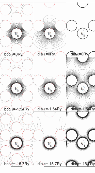
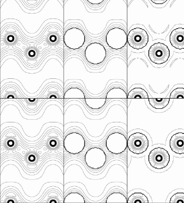
USWs look like the ones shown in Fig. 1. Here we have chosen $L\mathrm{=}0,$ which is the most appropriate for expanding charge densities. In the two first panels, we show the $s$-USW for six different USW sets, specifically sets with 3 different energies and for 2 different hard-sphere structures. The latter are body-centered cubic (bcc), which is closely packed, and diamond (dia), which is open and can be viewed as bcc with every second sphere removed to be part of the interstitial. In both structures, all spheres are equivalent. We see that the USW for the higher energies spread into the voids but, nevertheless, stays essentially inside its Voronoi (Wigner-Seitz) cell.

Because they are solutions of the wave equation (1), the USWs are invariant to a uniform scaling $\left(t\right)$ of the structure, provided that they are considered as functions of a dimensionless space variable $\mathbf{r/}t$ and the dimensionless energy variable $\varepsilon t^{2}.$


Refer to caption
Figure 1: (Color online) USW with $L=0$ from six different sets: The ones with $\varepsilon t^{2}=0$ (top), $-7.6$ (middle), or $-77$ (bottom) and the bcc structure (left) or the diamond structure (middle and right). Here, $t$ is the radius of touching spheres, i.e. half the nearest-neighbor distance. For diamond-structured silicon, $t=2.22$ Bohr radii and, for this case, the energies are therefore $\varepsilon=0$ (top), $-1.54$ (middle) or $-15.7$ Ry (bottom). The contours of the USW are in the (110) diagonal plane and range from 00 to $Y_{00}=1/\sqrt{4\pi}\approx 0.28$ in steps of 0.01. The (red) dots indicate the hard spheres whose radius was taken to be $a=0.8t$. In the bcc structure, the spheres are at the corners and body-centers of cubes. The diamond structure follows from bcc structure by deleting every second sphere, i.e. by including it in the interstitial. In both structures, all sites are equivalent (translationally in bcc, and with every second site inverted in dia), so that for a given structure and energy there is only one $s$-USW shape, $\psi_{s}$. It was generated from eq.s (19) and (30) by screening the bare spherical $s$-wave, $e^{-r\sqrt{-\varepsilon}}/r,$ with all waves centered at the $51$ (bcc) or $87$ (dia) nearest sites and having $l\leq l_{\max}=9$. This high value of $l_{\max}$ was chosen in order that the lowest contour display the hard spheres. The last panel shows the $s$-USW symmetrized with respect to the identity representation of the diamond space-group (Fd3m). The symmetrized USW with the lowest energy decays rapidly into the interstitial, the one with intermediate energy decays moderately fast, and the one with zero energy stays constant (see eq. (94) and Sect. VI.3.1). For the symmetrized $s$-USW, $l_{\max}=3$ suffices. See Sect.s II.2 and VI.2.

II.3 Taylor series in $r-a$ of the radial functions

In order to combine USW-sets with different energies linearly into a set of v&d functions, $\varrho_{dRL}\left(\mathbf{r}\right),$ with the super-unitary property (14), we need to expand the radial functions $f$ and $g$ defined in (17) and (18) in $\varepsilon$-dependent Taylor series in $r-a.$ Since the radial wave equation (6) is simplest when expressed in terms of $r$ times the radial function, it is convenient instead of $f$ and $g$ to use

$$U\left(\varepsilon,r\right)\equiv ru\left(\varepsilon,r\right)\equiv r\left[f\left(\varepsilon,r\right)-g\left(\varepsilon,r\right)\right]$$ (33)

and

$$G\left(\varepsilon,r\right)\equiv rg\left(\varepsilon,r\right),$$ (34)

because they satisfy the boundary conditions:

$$U\left(\varepsilon,a\right)=a,\;\;U^{\prime}\left(\varepsilon,a\right)=0,$$ (35)

and

$$G\left(\varepsilon,a\right)=0,\;\;G^{\prime}\left(\varepsilon,a\right)=1.$$ (36)

Here again, the subscripts $R$ and $l$ have been dropped for simplicity. The projection (16) of the USWs, expressed in the form needed for the definition of the v&d functions, is then:

$\displaystyle r\mathcal{\hat{P}}_{R^{\prime}L^{\prime}}\left(r\right)\psi_{RL}\left(\varepsilon,\mathbf{r}\right)$
$\displaystyle=ru_{R^{\prime}l^{\prime}}(\varepsilon,r)\delta_{R^{\prime}R}\delta_{L^{\prime}L}+rg_{R^{\prime}l^{\prime}}(\varepsilon,r)\mathcal{S}_{R^{\prime}L^{\prime},RL}\left(\varepsilon\right)$ (37)
$\displaystyle=U_{R^{\prime}l^{\prime}}(\varepsilon,r)\delta_{R^{\prime}R}\delta_{L^{\prime}L}+G_{R^{\prime}l^{\prime}}(\varepsilon,r)\mathcal{S}_{R^{\prime}L^{\prime},RL}\left(\varepsilon\right),$ (38)

where the script slope matrix is the one appropriate for $r\mathcal{\hat{P}}_{R^{\prime}L^{\prime}}\left(r\right)\psi_{RL}\left(\varepsilon,\mathbf{r}\right):$

$$\mathcal{S}_{R^{\prime}L^{\prime},RL}\left(\varepsilon\right)\equiv S_{R^{\prime}L^{\prime},RL}\left(\varepsilon\right)+\delta_{R^{\prime}R}\delta_{L^{\prime}L}$$ (39)

We now expand the $r$-dependence of the radial functions entering the projection (38) in an $\varepsilon$-dependent Taylor series in $r-a$ using the radial wave equation (6). For a radial solution, $\Psi\left(\varepsilon,r\right)\equiv r\psi\left(\varepsilon,r\right),$ with boundary conditions $\Psi\left(a\right)$ and $\Psi^{{}^{\prime}}\left(a\right)$ chosen to be independent of energy, the 2nd and 3rd radial derivatives are simply:

$\displaystyle\Psi^{\prime\prime}\left(\varepsilon,r\right)$ $\displaystyle=\left[w\left(r\right)-\varepsilon\right]\Psi\left(\varepsilon,r\right),\;\mathrm{and}$
$\displaystyle\Psi^{\prime\prime\prime}\left(\varepsilon,r\right)$ $\displaystyle=w^{\prime}\left(r\right)\Psi\left(\varepsilon,r\right)+\left[w\left(r\right)-\varepsilon\right]\Psi^{\prime}\left(\varepsilon,r\right)$

where $w\left(r\right)\equiv l\left(l+1\right)/r^{2}$ is the centrifugal potential. Using these derivatives for the functions with the boundary conditions (35) and (36), yield the following Taylor series:

$$U\left(\varepsilon,r\right)=a+a\left(w-\varepsilon\right)\frac{\left(r-a\right)^{2}}{2!}+aw^{\prime}\frac{\left(r-a\right)^{3}}{3!}+o$$ (40)

and

$$G\left(\varepsilon,r\right)=\left(r-a\right)+\left(w-\varepsilon\right)\frac{\left(r-a\right)^{3}}{3!}+o,$$ (41)

with $o$ as defined in (13). Moreover,

$$w\equiv\frac{l\left(l+1\right)}{a^{2}}\;\;\mathrm{and\;\;}aw^{\prime}\equiv-\frac{2l\left(l+1\right)}{a^{2}}$$ (42)

are respectively the value- and $a$ times the first derivative of the centrifugal potential at the hard sphere.

As an example, for $l=0,$ $w=0,$ so that $U_{s}\left(\varepsilon,r\right)/a$ is a function of $\left(r-a\right)^{2}\varepsilon$ and $G_{s}\left(\varepsilon,r\right)$ is an odd function of $\left(r-a\right)\sqrt{-\varepsilon}.$ In fact, $U_{s}\left(\varepsilon,r\right)=a\cosh\left\{\left(r-a\right)\sqrt{-\varepsilon}\right\}$ and $G_{s}\left(\varepsilon,r\right)=\sqrt{-\varepsilon}^{-1}\sinh\left\{\left(r-a\right)\sqrt{-\varepsilon}\right\}.$

II.4 Energy-divided differences

Next, we must form linear combinations with zero value, 1st, 2nd, and 3rd radial derivatives in all non-eigenchannels of the USW-sets with 4 different energies. This means: the projections formed from (38) of those linear combinations must have all terms with $R^{\prime}\neq R$ or $L^{\prime}\neq L$ smaller than $\left(r-a\right)^{3}.$ From eq.s (40) and (41) we see that the second and higher energy derivatives of $U\left(\varepsilon,r\right)$ and $G\left(\varepsilon,r\right)$ are smaller than $\left(r-a\right)^{3},$ and differentiation of the USWs in eq. (38) with respect to energy can therefore be used to single out functions which satisfy equations (14).

Rather than using derivatives at one energy, it is far more flexible and accurate to use energy-divided differences for discrete sets of energies. From the theory of polynomial approximation (Newton-Lagrange), remember that if we approximate a function of energy, $\psi\left(\varepsilon\right),$ by the polynomial of $d$th order which coincides with $\psi\left(\varepsilon\right)$ at the energies $\epsilon_{1},..,\epsilon_{d+1},$ then the highest non-vanishing energy derivative –the $d$th– of this polynomial is $d!$ times the $d$th divided difference. The latter can be written in many ways, but the most general and compact is 00DivDif :

$$\sum_{n=1}^{d+1}\frac{\psi\left(\epsilon_{n}\right)}{\Pi_{m=1,\neq n}^{d+1}\left(\epsilon_{n}-\epsilon_{m}\right)}\equiv\psi_{1..d+1}\,.$$ (43)

On the right-hand side we have introduced a notation according to which the value (the 0th divided difference), $\psi\left(\epsilon_{n}\right),$ at $\epsilon_{n}$ is denoted $\psi_{n}.$ The first divided difference,

$$\frac{\psi\left(\epsilon_{m}\right)-\psi\left(\epsilon_{n}\right)}{\epsilon_{m}-\epsilon_{n}}=\frac{\psi_{m}-\psi_{n}}{\epsilon_{m}-\epsilon_{n}},$$

taken at the two energy points, $\epsilon_{m}$ and $\epsilon_{n},$ is denoted $\psi_{mn}$ like in eq. (5). The second divided difference,

$$\frac{\frac{\psi\left(\epsilon_{l}\right)-\psi\left(\epsilon_{m}\right)}{\epsilon_{l}-\epsilon_{m}}-\frac{\psi\left(\epsilon_{m}\right)-\psi\left(\epsilon_{n}\right)}{\epsilon_{m}-\epsilon_{n}}}{\epsilon_{l}-\epsilon_{n}}=\frac{\psi_{lm}-\psi_{mn}}{\epsilon_{l}-\epsilon_{n}},$$

taken at the three energy points, $\epsilon_{l},$ $\epsilon_{m},$ and $\epsilon_{n},$ is denoted $\psi_{lmn}.$ Hence, the general notation is:

$$\frac{\psi_{m,m+1,...,n}-\psi_{m+1,...,n,n+1}}{\epsilon_{m}-\epsilon_{n+1}}\equiv\psi_{m,m+1,..,n,n+1}.$$

Note that a divided difference (43) depends on the energy points at which it is formed, but not on their order, e.g. $\psi_{lmn}=\psi_{nlm}.$

If $\psi\left(\varepsilon\right)$ itself is a polynomial of order $d,$ then all divided differences formed for more than $d+1$ energies, i.e. of order higher than $d,$ vanish. From eq.s (40) and (41), therefore, all the second and higher energy-divided differences of the functions $U\left(\varepsilon,r\right)$ and $G\left(\varepsilon,r\right)$ are smaller than $\left(r-a\right)^{3}.$ The energy-divided differences of increasing order are seen to be:

$\displaystyle U_{n}\left(r\right)$ $\displaystyle=a-a\left(\epsilon_{n}-w\right)\frac{\left(r-a\right)^{2}}{2!}$
$\displaystyle+aw^{\prime}\frac{\left(r-a\right)^{3}}{3!}+o,$ (44)
$\displaystyle U_{mn}\left(r\right)$ $\displaystyle=-a\frac{\left(r-a\right)^{2}}{2!}+o,$ (45)
$\displaystyle U_{lmn..}\left(r\right)$ $\displaystyle=o,$ (46)

with $o$ defined in (13), and:

$\displaystyle G_{n}\left(r\right)$ $\displaystyle=\left(r-a\right)-\left(\epsilon_{n}-w\right)\frac{\left(r-a\right)^{3}}{3!}+o,$ (47)
$\displaystyle G_{mn}\left(r\right)$ $\displaystyle=-\frac{\left(r-a\right)^{3}}{3!}+o,$ (48)
$\displaystyle G_{lmn}..\left(r\right)$ $\displaystyle=o.$ (49)

In the following, e.g. in eq. (51) below, we shall be using that the $d$th-order divided difference of a product is given by the binomial rule 00DivDif :

$$\left(G\mathcal{S}\right)_{1...d+1}=\sum_{m=1}^{d+1}G_{1..m}\,\mathcal{S}_{m.d+1}.$$ (50)

III V&d functions

After these preliminaries, we are finally in a position form the set of v&d functions, $\varrho_{dRL}\left(\mathbf{r}\right),$ with the super-unitary property (14) from the four sets of USWs, $\psi_{RL}\left(\epsilon_{n},\mathbf{r}\right)$ with $n=1,2,3,4,$ or – more conveniently – from the set of four energy-divided differences: $\psi_{1;RL}\left(\mathbf{r}\right),$ $\psi_{12;RL}\left(\mathbf{r}\right),$ $\psi_{123;RL}\left(\mathbf{r}\right),$ and $\psi_{1234;RL}\left(\mathbf{r}\right).$

Since energy-divided differences are formed for a given element of a vector or a matrix, we can avoid the $R^{\prime}L^{\prime}$ and $R^{\prime}L^{\prime},RL$ subscripts by using a matrix notation in which the projection (38) is written as: $r\mathcal{\hat{P}}\left(r\right)\psi\left(\varepsilon,\mathbf{r}\right)=U(\varepsilon,r)1+G(\varepsilon,r)\mathcal{S}\left(\varepsilon\right).$ Forming energy-divided differences of increasing order – from 0th to 3rd – by use of the binomial formula (50) then yields:

$\displaystyle r\mathcal{\hat{P}}\left(r\right)\psi_{1}\left(\mathbf{r}\right)$ $\displaystyle=U_{1}\left(r\right)1+G_{1}\left(r\right)\mathcal{S}_{1},$
$\displaystyle r\mathcal{\hat{P}}\left(r\right)\psi_{12}\left(\mathbf{r}\right)$ $\displaystyle=U_{12}\left(r\right)1+G_{1}\left(r\right)S_{12}+G_{12}\left(r\right)\mathcal{S}_{2},$
$\displaystyle r\mathcal{\hat{P}}\left(r\right)\psi_{123}\left(\mathbf{r}\right)$ $\displaystyle=G_{1}\left(r\right)S_{123}+G_{12}\left(r\right)S_{23}+o,$
$\displaystyle r\mathcal{\hat{P}}\left(r\right)\psi_{1234}\left(\mathbf{r}\right)$ $\displaystyle=G_{1}\left(r\right)S_{1234}+G_{12}\left(r\right)S_{234}+o.$ (51)

Here, we have chosen to use the energy point with the lower index first, e.g. $\epsilon_{1}$ before $\epsilon_{2}.$ Moreover, we have used that the energy-divided differences, except the 0th, of the slope matrices $\mathcal{S}\left(\varepsilon\right)$ and $S\left(\varepsilon\right)$ are identical because they differ by merely a constant (see eq. (39)). Most importantly, we have made use of eq.s (46) and (49).

The set of 3rd-derivative functions, $\varrho_{3}\left(\mathbf{r}\right),$ is seen from eq.s (14) and (48) to have the projection $-G_{12}\left(r\right)1.$ We therefore eliminate $G_{1}\left(r\right)$ from the last two equations (51):

$\displaystyle r\mathcal{\hat{P}}\left(r\right)\psi_{1234}\left(\mathbf{r}\right)\left(S_{1234}\right)^{-1}-r\mathcal{\hat{P}}\left(r\right)\psi_{123}\left(\mathbf{r}\right)\left(S_{123}\right)^{-1}$
$\displaystyle=G_{12}\left(r\right)\left[S_{234}\left(S_{1234}\right)^{-1}-S_{23}\left(S_{123}\right)^{-1}\right]+o,$ (52)

and find that:

$\displaystyle\varrho_{3}\left(\mathbf{r}\right)$ $\displaystyle=-\psi_{123}\left(\mathbf{r}\right)\left[S_{23}-S_{234}\left(S_{1234}\right)^{-1}S_{123}\right]^{-1}$
$\displaystyle-\psi_{1234}\left(\mathbf{r}\right)\left[S_{234}-S_{23}\left(S_{123}\right)^{-1}S_{1234}\right]^{-1}$ (53)
$\displaystyle\equiv\psi_{123}\left(\mathbf{r}\right)D_{3,3}+\psi_{1234}\left(\mathbf{r}\right)D_{4,3}.$

Here we have used that in the matrix notation, the projection of a linear combination $\sum_{RL}\psi_{1.n;RL}\left(\mathbf{r}\right)c_{RL}$ equals the projection of $\psi_{1.n;RL}\left(\mathbf{r}\right)$ right-multiplied by $c_{RL}.$ In eq. (52) and in the following, functions like $\psi_{123}\left(\mathbf{r}\right)$ and $\varrho_{3}\left(\mathbf{r}\right)$ are row vectors with the respective components $\varrho_{3;R^{\prime}L^{\prime}}\left(\mathbf{r}\right)$ and $\psi_{123;RL}\left(\mathbf{r}\right),$ while constants like $\left[S_{23}-S_{234}\left(S_{1234}\right)^{-1}S_{123}\right]^{-1}$ are square matrices with $RL,R^{\prime}L^{\prime}$-elements. Hence, the subscripts $RL$ are summed over, and the square parentheses in eq. (53) contain matrix products and inversions. In the last line of eq. (53) and in the following, a matrix $D_{n,d}$ with elements $D_{nR^{\prime}L^{\prime},dRL}$ is defined to be the coefficient to $\psi_{1.n}\left(\mathbf{r}\right)$ in the expansion of $\varrho_{d}\left(\mathbf{r}\right).$ Remember, that we have chosen to number the energy points, $n=1,..,4,$ and the radial derivatives, $d=0,..,\,3.$

In order to find the set of 1st-derivative functions, we eliminate $G_{12}\left(r\right)$ from the last two equations (51) and subsequently insert expression (47) for $G_{1}\left(r\right)$:

$\displaystyle r\mathcal{\hat{P}}\left(r\right)\left\{\psi_{1234}\left(\mathbf{r}\right)\left(S_{234}\right)^{-1}-\psi_{123}\left(\mathbf{r}\right)\left(S_{23}\right)^{-1}\right\}$
$\displaystyle=G_{1}\left(r\right)\left[S_{1234}\left(S_{234}\right)^{-1}-S_{123}\left(S_{23}\right)^{-1}\right]+o$
$\displaystyle=\left[\left(r-a\right)-\frac{\left(r-a\right)^{3}}{3!}\left(\epsilon_{1}-w\right)\right]$
$\displaystyle\qquad\times\left[S_{1234}\left(S_{234}\right)^{-1}-S_{123}\left(S_{23}\right)^{-1}\right]+o.$ (54)

As a result:

$\displaystyle\varrho_{1}\left(\mathbf{r}\right)$ $\displaystyle=\varrho_{3}\left(\mathbf{r}\right)\left(\epsilon_{1}-w\right)$
$\displaystyle+\left[\psi_{1234}\left(\mathbf{r}\right)\left(S_{234}\right)^{-1}-\psi_{123}\left(\mathbf{r}\right)\left(S_{23}\right)^{-1}\right]$
$\displaystyle\times\left[S_{1234}\left(S_{234}\right)^{-1}-S_{123}\left(S_{23}\right)^{-1}\right]^{-1}$
$\displaystyle=\psi_{123}\left(\mathbf{r}\right)D_{3,3}\left[S_{234}\left(S_{1234}\right)^{-1}+\epsilon_{1}-w\right]$
$\displaystyle+\psi_{1234}\left(\mathbf{r}\right)D_{4,3}\left[S_{23}\left(S_{123}\right)^{-1}+\epsilon_{1}-w\right].$ (55)

As usual, quantities like $\epsilon_{1}-w$ are diagonal matrices.

The set of 2nd-derivative functions, $\varrho_{2}\left(\mathbf{r}\right),$ is seen from eq.s (14) and (45) to have the projection $-U_{12}\left(r\right)\frac{1}{a}.$ From the second equation (51) and from expressions (52) and (54) therefore:

$\displaystyle\varrho_{2}\left(\mathbf{r}\right)a=-\psi_{12}\left(\mathbf{r}\right)-\psi_{123}\left(\mathbf{r}\right)$
$\displaystyle\times\left\{\begin{array}[c]{c}\left(S_{23}\right)^{-1}\left[S_{1234}\left(S_{234}\right)^{-1}-S_{123}\left(S_{23}\right)^{-1}\right]^{-1}S_{12}\\ +\left(S_{123}\right)^{-1}\left[S_{234}\left(S_{1234}\right)^{-1}-S_{23}\left(S_{123}\right)^{-1}\right]^{-1}\mathcal{S}_{2}\end{array}\right\}$
$\displaystyle+\psi_{1234}\left(\mathbf{r}\right)$
$\displaystyle\times\left\{\begin{array}[c]{c}\left(S_{234}\right)^{-1}\left[S_{1234}\left(S_{234}\right)^{-1}-S_{123}\left(S_{23}\right)^{-1}\right]^{-1}S_{12}\\ +\left(S_{1234}\right)^{-1}\left[S_{234}\left(S_{1234}\right)^{-1}-S_{23}\left(S_{123}\right)^{-1}\right]^{-1}\mathcal{S}_{2}\end{array}\right\},$

which reduces to:

$\displaystyle\varrho_{2}\left(\mathbf{r}\right)a$ $\displaystyle=-\psi_{12}\left(\mathbf{r}\right)$
$\displaystyle-\psi_{123}\left(\mathbf{r}\right)D_{3,3}\left[\mathcal{S}_{2}-S_{234}\left(S_{1234}\right)^{-1}S_{12}\right]$
$\displaystyle-\psi_{1234}\left(\mathbf{r}\right)D_{4,3}\left[\mathcal{S}_{2}-S_{23}\left(S_{123}\right)^{-1}S_{12}\right].$ (56)

Of the divided-difference functions, $\psi_{1..d+1}\left(\mathbf{r}\right),$ only the 0th does not vanish at all spheres, and it must therefore be included in the value functions $\varrho_{0}\left(\mathbf{r}\right).$ From the first eq. (51) and eq. (44):

$\displaystyle r\mathcal{\hat{P}}\left(r\right)\psi_{1}\left(\mathbf{r}\right)$ $\displaystyle=a-\frac{\left(r-a\right)^{2}}{2!}a\left(\epsilon_{1}-w\right)$
$\displaystyle+\frac{\left(r-a\right)^{3}}{3!}aw^{\prime}+G_{1}\left(r\right)\mathcal{S}_{1}+o,$

so that with the help of the first lines of expressions (54) and (55), we get:

$\displaystyle\psi_{1}\left(\mathbf{r}\right)$ $\displaystyle=\varrho_{0}\left(\mathbf{r}\right)a-\varrho_{2}\left(\mathbf{r}\right)a\left(\epsilon_{1}-w\right)+\varrho_{3}\left(\mathbf{r}\right)aw^{\prime}$
$\displaystyle+\left[\varrho_{1}\left(\mathbf{r}\right)-\varrho_{3}\left(\mathbf{r}\right)\left(\epsilon_{1}-w\right)\right]\mathcal{S}_{1}.$

As a result, the set of value functions is given by:

$\displaystyle\varrho_{0}\left(\mathbf{r}\right)a$ $\displaystyle=\psi_{1}\left(\mathbf{r}\right)-\psi_{12}\left(\mathbf{r}\right)\left(\epsilon_{1}-w\right)+\psi_{123}\left(\mathbf{r}\right)$
$\displaystyle\times\left\{\begin{array}[c]{c}\left[S_{23}-S_{234}\left(S_{1234}\right)^{-1}S_{123}\right]^{-1}\\ \times\left[\mathcal{S}_{2}-S_{234}\left(S_{1234}\right)^{-1}S_{12}\right]\left(\epsilon_{1}-w\right)\\ +\left[S_{23}-S_{234}\left(S_{1234}\right)^{-1}S_{123}\right]^{-1}aw^{\prime}\\ -\left[S_{123}-S_{1234}\left(S_{234}\right)^{-1}S_{23}\right]^{-1}\mathcal{S}_{1}\end{array}\right\}$
$\displaystyle+\psi_{1234}\left(\mathbf{r}\right)$
$\displaystyle\times\left\{\begin{array}[c]{c}\left[S_{234}-S_{23}\left(S_{123}\right)^{-1}S_{1234}\right]^{-1}\\ \times\left[\mathcal{S}_{2}-S_{23}\left(S_{123}\right)^{-1}S_{12}\right]\left(\epsilon_{1}-w\right)\\ +\left[S_{234}-S_{23}\left(S_{123}\right)^{-1}S_{1234}\right]^{-1}aw^{\prime}\\ -\left[S_{1234}-S_{123}\left(S_{23}\right)^{-1}S_{234}\right]^{-1}\mathcal{S}_{1}\end{array}\right\},$

which simplifies to:

$\displaystyle\varrho_{0}\left(\mathbf{r}\right)a$
$\displaystyle=\psi_{1}\left(\mathbf{r}\right)-\psi_{12}\left(\mathbf{r}\right)\left(\epsilon_{1}-w\right)$
$\displaystyle-\psi_{123}\left(\mathbf{r}\right)D_{3,3}\left\{\begin{array}[c]{c}aw^{\prime}+\mathcal{S}_{2}\left(\epsilon_{1}-w\right)+\\ S_{234}\left(S_{1234}\right)^{-1}\left[\mathcal{S}_{1}-S_{12}\left(\epsilon_{1}-w\right)\right]\end{array}\right\}$ (59)
$\displaystyle-\psi_{1234}\left(\mathbf{r}\right)D_{4,3}\left\{\begin{array}[c]{c}aw^{\prime}+\mathcal{S}_{2}\left(\epsilon_{1}-w\right)+\\ S_{23}\left(S_{123}\right)^{-1}\left[\mathcal{S}_{1}-S_{12}\left(\epsilon_{1}-w\right)\right]\end{array}\right\}.$ (62)

Hence, for use in the interpolation (8), we have succeeded in forming a set of four v&d functions, $\varrho_{d}\left(\mathbf{r}\right)$ with $d\mathrm{=}0$ to $3,$ from the USW-sets at four different energies, $\psi_{n}\left(\mathbf{r}\right)\equiv\psi\left(\epsilon_{n},\mathbf{r}\right)\,$with $n\mathrm{=}1$ to $4.$ The result is:

$\displaystyle\varrho_{dRL}\left(\mathbf{r}\right)$ $\displaystyle=\sum_{n=1}^{4}\sum_{R^{\prime}L^{\prime}}\sum_{n^{\prime}=1}^{n}\frac{\psi_{n^{\prime}R^{\prime}L^{\prime}}\left(\mathbf{r}\right)}{\Pi_{m=1,\neq n^{\prime}}^{n}\left(\epsilon_{n^{\prime}}-\epsilon_{m}\right)}\,D_{nR^{\prime}L^{\prime},dRL}$
$\displaystyle=\sum_{n=1}^{4}\sum_{R^{\prime}L^{\prime}}\psi_{1..n;R^{\prime}L^{\prime}}\left(\mathbf{r}\right)\,D_{nR^{\prime}L^{\prime},dRL}.$ (63)

The similarity transformation, $D_{n,d},$ from the four energy-divided differences (43) of USWs, $\psi_{1..n}\left(\mathbf{r}\right),$ to the v&d functions, $\varrho_{d}\left(\mathbf{r}\right),$ is given by the coefficients found in eq.s (53), (55), (56), and (62) in terms of energy-divided differences $\mathcal{S}_{1..n}$ of the screened structure matrix (39). For the odd and even derivatives’ functions they are respectively:

$\displaystyle D_{1,3}$ $\displaystyle=D_{2,3}=0,$
$\displaystyle D_{3,3}$ $\displaystyle=-\left[S_{23}-S_{234}\left(S_{1234}\right)^{-1}S_{123}\right]^{-1},$
$\displaystyle D_{4,3}$ $\displaystyle=-\left[S_{234}-S_{23}\left(S_{123}\right)^{-1}S_{1234}\right]^{-1}$
$\displaystyle=-\left(S_{1234}\right)^{-1}S_{123}D_{3,3},$
$\displaystyle D_{1,1}$ $\displaystyle=D_{2,1}=0,$
$\displaystyle D_{3,1}$ $\displaystyle=D_{3,3}\left[S_{234}\left(S_{1234}\right)^{-1}+\epsilon_{1}-w\right],$
$\displaystyle D_{4,1}$ $\displaystyle=D_{4,3}\left[S_{23}\left(S_{123}\right)^{-1}+\epsilon_{1}-w\right]$
$\displaystyle=A-\left(S_{1234}\right)^{-1}S_{123}D_{3,3}\left(\epsilon_{1}-w\right),$ (64)

and:

$\displaystyle D_{1,2}a$ $\displaystyle=0,$
$\displaystyle D_{2,2}a$ $\displaystyle=-1,$
$\displaystyle D_{3,2}a$ $\displaystyle=-D_{3,3}\left[\mathcal{S}_{2}-S_{234}\left(S_{1234}\right)^{-1}S_{12}\right],$
$\displaystyle D_{4,2}a$ $\displaystyle=-D_{4,3}\left[\mathcal{S}_{2}-S_{23}\left(S_{123}\right)^{-1}S_{12}\right]=-D_{4,3}\mathcal{S}_{2}+AS_{12},$
$\displaystyle D_{1,0}a$ $\displaystyle=1,$
$\displaystyle D_{2,0}a$ $\displaystyle=-\left(\epsilon_{1}-w\right),$
$\displaystyle D_{3,0}a$ $\displaystyle=-D_{3,3}\left\{\begin{array}[c]{c}aw^{\prime}+\mathcal{S}_{2}\left(\epsilon_{1}-w\right)+\\ S_{234}\left(S_{1234}\right)^{-1}\left[\mathcal{S}_{1}-S_{12}\left(\epsilon_{1}-w\right)\right]\end{array}\right\},$ (67)
$\displaystyle D_{4,0}a$ $\displaystyle=-D_{4,3}\left\{\begin{array}[c]{c}aw^{\prime}+\mathcal{S}_{2}\left(\epsilon_{1}-w\right)+\\ S_{23}\left(S_{123}\right)^{-1}\left[\mathcal{S}_{1}-S_{12}\left(\epsilon_{1}-w\right)\right]\end{array}\right\}$ (70)
$\displaystyle=-D_{4,3}\left\{aw^{\prime}+\mathcal{S}_{2}\left(\epsilon_{1}-w\right)\right\}-A\left\{\mathcal{S}_{1}-S_{12}\left(\epsilon_{1}-w\right)\right\}.$ (71)

Here, we have defined the matrix:

$$A\equiv D_{4,3}S_{23}\left(S_{123}\right)^{-1}=\left[S_{1234}-S_{123}\left(S_{23}\right)^{-1}S_{234}\right]^{-1},$$ (72)

and $\epsilon_{1}-w$ and $aw^{\prime}$ are diagonal matrices with the respective components $\epsilon_{1}-l\left(l+1\right)\left(a_{R}\right)^{-2}$ and $-2l\left(l+1\right)\left(a_{R}\right)^{-2}.$ Expressions involving inversion of the second divided difference, $S_{123}$, which may not be positive definite, have been rewritten in terms of inverted first and the third divided differences, $S_{23}$ and $S_{1234}.$ The latter are likely to be positive-definite because, as seen from eq. (93) in Sect. V, their elements are overlap integrals over nearly identical functions.

It should be noted, that the v&d functions are invariant to the numbering of the four energies.

Here, we have chosen to express the v&d functions in terms of the dimensionless slope matrix, $\mathcal{S}\left(\varepsilon\right)$ given by eq.s (39) and (31), because it has a simple physical interpretation. To rewrite eq.s (64) and (71) in terms of the symmetric matrix $a\mathcal{S}$ is a trivial matter.

In order to generate all 16 submatrices (64)-(71), one thus needs to invert 4 matrices, e.g. $S_{1234},$ $S_{23}-S_{234}\left(S_{1234}\right)^{-1}S_{123},$ $S_{23},$ and $S_{1234}-S_{123}\left(S_{23}\right)^{-1}S_{234},$ in addition to the 4 matrices $B\left(\epsilon_{n}\right)+n(\epsilon_{n},a)/j(\epsilon_{n},a)$ in eq. (31). The remaining matrix operations in eq.s (64) and (71) are merely products and sums. The dimensions of the matrices will be discussed in Sect.s VI.1 and VI.2.

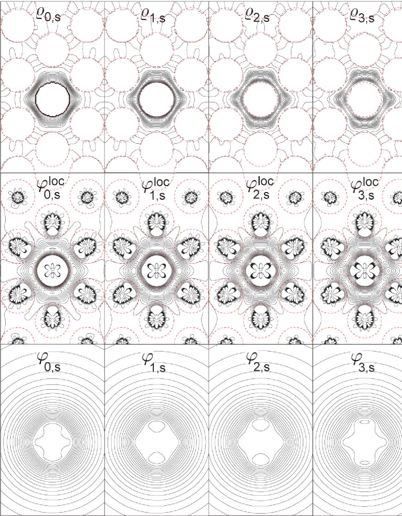
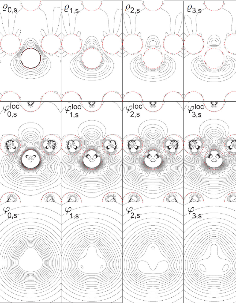
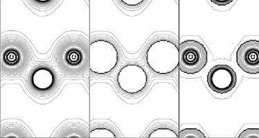
This value-and-first-3-derives’ formalism achieves to invert 4 slope matrices instead of one, four times larger matrix. Apart from this, the 4 v&d functions of a given $RL$ are more localized than the 4 USWs of the same $RL$ because any v&d function has vanishing values and first 3 radial derivatives at all spheres other than its own. Moreover, with increasing derivative order, $d,$ the v&d function, $\varrho_{dRL}\left(\mathbf{r}\right),$ extends further and further into the interstitial around site $R,$ at the same time as remaining localized to inside the Voronoi cell, approximately. This can clearly be seen in the top row of Fig.s 2 and 3, where we show the value-, first-, second-, and third-derivative $s$-functions for bcc- and dia-structured interstitials.

The interpolation (8) is local, that is: to the density at point $\mathbf{r,}$ essentially only the v&d functions centered at the cell containing $\mathbf{r}$ contribute. However, the generation of the v&d functions is not local. They are multi-centered linear combinations (63) of USWs which, themselves, are multi-centered linear combinations (19) of Hankel functions. This generation of shorter-ranged functions from longer-ranged ones – and even in two stages – was used to produce the contour plots in Fig.s 2 and 3. For the purpose of simplifying the plotting of $\rho\left(\mathbf{r}\right)$ from eq. (8), one might use v&d functions tabulated on a mesh spanning their own cell and its near neighborhood. Faster, but less accurate, it is to approximate the v&d functions in the interstitial near an arbitrary site $\mathbf{R}^{\prime}$ by their cubic-harmonic expansion around that site:

$$\rho\left(\mathbf{r}\right)\approx\sum_{L^{\prime}}Y_{L^{\prime}}\left(\mathbf{\hat{r}}_{R^{\prime}}\right)\,\sum_{dL}\mathcal{\hat{P}}_{R^{\prime}L^{\prime}}\left(r_{R^{\prime}}\right)\varrho_{dRL}\left(\mathbf{r}\right)\mathcal{R}_{RL}^{\left(d\right)}$$ (73)

This one-center expansion (73) is less useful for open than for close-packed structures because it is strictly valid only for $a_{R^{\prime}}\leq r_{R^{\prime}}\leq\min_{R^{\prime\prime}}\left(d_{R^{\prime\prime}R^{\prime}}-a_{R^{\prime}}\right),$ where the latter is the distance to the nearest-neighbor sphere. For $\min_{R^{\prime\prime}}\left(d_{R^{\prime\prime}R^{\prime}}-a_{R^{\prime}}\right)\leq r_{R^{\prime}}<\min_{R^{\prime\prime}}d_{R^{\prime\prime}R^{\prime}},$ the expansion converges to the superposition of Hankel functions. Approximating the v&d functions by the cubic-harmonic expansion around the own site, i.e. choosing $\mathbf{R}^{\prime}=\mathbf{R,}$ brings great simplification, but only for close-packed structures, does the expansion hold throughout the Voronoi cell. The radial functions, $\mathcal{\hat{P}}_{R^{\prime}L^{\prime}}\left(r\right)\varrho_{dRL}\left(\mathbf{r}\right),$ will be derived in the Appendix.

The alert reader will have noted that $\varrho_{d=0\,s}\left(\mathbf{r}\right)$ in Figs 2 and 3 does not start out flat from the central sphere, but like $1/r.$ This is because we have chosen to carry the prefactor $r$ in the boundary condition (14) for the v&d functions in order to simplify the formalism leading to eq.s (63)-(72). So what starts out flat, is $r$ times the spherical average of $\varrho_{d=0\,s}\left(\mathbf{r}\right)$. Having found these v&d functions, we may of course form those, $\bar{\varrho}_{dRL}\left(\mathbf{r}\right),$ which satisfy the boundary conditions without the prefactor $r$:

$$\mathcal{\hat{P}}_{R^{\prime}L^{\prime}}\left(r\right)\bar{\varrho}_{dRL}\left(\mathbf{r}\right)=\frac{\left(r-a_{R}\right)^{d}}{d!}\delta_{R^{\prime}R}\delta_{L^{\prime}L}+o.$$ (74)

The result, most easily obtained by using the interpolation formalism (7)-(8) with $\rho\left(\mathbf{r}\right)=\bar{\varrho}_{dRL}\left(\mathbf{r}\right),$ is:

$$\bar{\varrho}_{dRL}\left(\mathbf{r}\right)=\varrho_{dRL}\left(\mathbf{r}\right)a_{R}+\left(d+1\right)\varrho_{\left(d+1\right)RL}\left(\mathbf{r}\right),$$ (75)

with $\varrho_{d>d_{\max}\,RL}\left(\mathbf{r}\right)\equiv 0.$

The v&d functions are independent of the scale $\left(t\right)$ of the structure, provided that spatial derivatives are defined with respect to the dimensionless variable $\mathbf{r/}t$ and that the energy mesh times $t^{2}$ is kept constant. This follows from the fact that USWs solve the wave equation (1).

The main use of expressions (63)-(72) for the v&d functions as multi-centered linear combinations of USWs is for solving Poisson’s equation and for forming integrals, as we shall see in Sect.s IV and V.


Refer to caption
Figure 2: (Color online) Bcc structure as in the left-hand panel of Fig. 1. Top row: Value-, first-, second-, and third-derivative $s$-like functions, $\varrho_{ds}\left(\mathbf{r}\right)/\left\langle\varrho_{ds}\right\rangle$, normalized over the interstitial. See Sect. III. Middle row: Their localized potentials, $\varphi_{ds}^{loc}\left(\mathbf{r}\right)/\left\langle\varrho_{ds}\right\rangle.$ Bottom row: Their regular potentials, $\varphi_{ds}\left(\mathbf{r}\right)/\left\langle\varrho_{ds}\right\rangle.$ See Sect. IV.2. The localized potentials are screened by multipoles at the centers of the hard spheres and therefore diverge there. The regular potentials have these multipoles subtracted out. For $r$ large, all four regular potentials become that of a point charge, $-2/r$. The values of the normalization integrals are: $\left\langle\varrho_{ds}\right\rangle=\,$5.82, 2.05, 0.358, and 0.0256 (Bohr radii)d-2 for $d\,$= 0, 1, 2, and 3, respectively. The contours for the normalized v&d functions go from 00 to $0.03$ in steps of $0.002$ (Bohr radii)${}^{-3},$ those for the localized potentials from $-0.06$ upwards in steps of $0.012$ Ry, the zero-potential contour being the one following the hard spheres most closely, and those for the regular potentials from 0 to 0.99 in steps of 0.03 Ry. The energy mesh is exponential (eq. (105)) with the highest and lowest energies the same as those used in Fig. 1, i.e. $\epsilon_{1}=-1.54$ and $\epsilon_{4}=-15.7$ Ry.

Refer to caption
Figure 3: (Color online) Same as Fig. 2, but for the diamond-structure with the same nearest-neighbor distance as in Fig. 2. $\left\langle\varrho_{ds}\right\rangle=$ 11.25, 6.94, 1.89, and 0.188 (Bohr radii)d-2 for $d\,$= 0, 1, 2, and 3, respectively.

IV Solving Poisson’s equation

IV.1 Potentials from energy-divided differences of USWs

Poisson’s equation (2) for a charge density which is a spherical wave, $\rho\left(\mathbf{r}\right)=\psi\left(\varepsilon,\mathbf{r}\right),$ has the particular solution $V\left(\mathbf{r}\right)=8\pi\psi\left(\varepsilon,\mathbf{r}\right)/\varepsilon.$ For a charge density which is the $d$th energy-divided difference (43) of an USW, Poisson’s equation therefore has the solution

$\displaystyle-8\pi\Delta^{-1}\psi_{1..d+1;RL}\left(\mathbf{r}\right)=\sum_{n=1}^{d+1}\frac{8\pi\psi_{nRL}\left(\mathbf{r}\right)/\epsilon_{n}}{\Pi_{m=1,\neq n}^{d+1}\left(\epsilon_{n}-\epsilon_{m}\right)}$
$\displaystyle=\sum_{n=0}^{d+1}\frac{8\pi\psi_{nRL}\left(\mathbf{r}\right)}{\Pi_{m=0,\neq n}^{d+1}\left(\epsilon_{n}-\epsilon_{m}\right)}-\frac{8\pi\psi_{RL}\left(0,\mathbf{r}\right)}{\Pi_{m=1}^{d+1}\left(-\epsilon_{m}\right)}$
$\displaystyle=8\pi\psi_{0...d+1;RL}\left(\mathbf{r}\right)-\frac{8\pi\psi_{RL}\left(0,\mathbf{r}\right)}{\Pi_{m=1}^{d+1}\left(-\epsilon_{m}\right)}$ (76)

in the interstitial between the spheres. In the first term on the right-hand side, we have defined

$$\epsilon_{0}\equiv 0,$$ (77)

and have used this energy point to take the divided difference for the potential one order higher than for the charge density.

Inside the spheres, the solution (76) is joined smoothly to a solution of the Laplace equation.

IV.1.1 The localized potential

The second term, $-8\pi\psi_{RL}\left(0,\mathbf{r}\right)\left/\left(-\epsilon_{1}\right)..\left(-\epsilon_{d+1}\right)\right.,$ in expression (76) satisfies the Laplace equation. We can therefore choose merely the first term:

$$8\pi\psi_{0...d+1;RL}\left(\mathbf{r}\right)\equiv\phi_{1..d+1;RL}^{loc}\left(\mathbf{r}\right),$$ (78)

as the particular solution VPhiphi of interest in the interstitial. This choice makes the potential localized to the neighborhood of its own sphere because $\psi_{0...d+1;RL}\left(\mathbf{r}\right)$ is an energy-divided difference of at least 1st order and therefore has vanishing $L^{\prime}$-averages at all spheres for all $l^{\prime}\leq l_{\max}.$ This holds also for the eigen-projection of $\psi_{0...d+1;RL}\left(\mathbf{r}\right)$ because the eigen-projection of $\psi_{RL}\left(\varepsilon,\mathbf{r}\right)$ is $Y_{L}\left(\mathbf{\hat{r}}_{R}\right)$, independently of the energy. Near the own sphere, the localized potential has pure $L$-character.

The localized potential may be expanded around any site $\mathbf{R}^{\prime}$ in cubic-harmonics times radial functions:

$$\phi_{1..d+1;RL}^{loc}\left(\mathbf{r}\right)\approx 8\pi\sum_{L^{\prime}}Y_{L^{\prime}}\left(\mathbf{\hat{r}}_{R^{\prime}}\right)\mathcal{\hat{P}}_{R^{\prime}L^{\prime}}\left(r\right)\psi_{0...d+1;RL}\left(\mathbf{r}\right)$$ (79)

valid in the interstitial at and outside the $R^{\prime}$-sphere. Since $R^{\prime}L^{\prime}$-projection and forming energy-divided differences commute, we can reverse the order and use the binomial rule (50) to form the differences of the projections (37) expressed as $\mathcal{\hat{P}}\left(r\right)\psi\left(\varepsilon,\mathbf{r}\right)=u\left(\varepsilon,r\right)+g\left(\varepsilon,r\right)\mathcal{S}\left(\varepsilon\right).$ The resulting projections are for $d\mathrm{=}0$ to 3:

$\displaystyle\mathcal{\hat{P}}\left(r\right)\psi_{01}\left(\mathbf{r}\right)$ $\displaystyle=u_{01}\left(r\right)+g_{0}\left(r\right)S_{01}+g_{01}\left(r\right)\mathcal{S}_{1},$
$\displaystyle\mathcal{\hat{P}}\left(r\right)\psi_{012}\left(\mathbf{r}\right)$ $\displaystyle=u_{012}\left(r\right)+g_{0}\left(r\right)S_{012}$
$\displaystyle+g_{01}\left(r\right)S_{12}+g_{012}\left(r\right)\mathcal{S}_{2},$
$\displaystyle\mathcal{\hat{P}}\left(r\right)\psi_{0123}\left(\mathbf{r}\right)$ $\displaystyle=u_{0123}\left(r\right)+g_{0}\left(r\right)S_{0123}+g_{01}\left(r\right)S_{123}$
$\displaystyle+g_{012}\left(r\right)S_{23}+g_{0123}\left(r\right)\mathcal{S}_{3},$
$\displaystyle\mathcal{\hat{P}}\left(r\right)\psi_{01234}\left(\mathbf{r}\right)$ $\displaystyle=u_{01234}\left(r\right)+g_{0}\left(r\right)S_{01234}$
$\displaystyle+g_{01}\left(r\right)S_{1234}+g_{012}\left(r\right)S_{234}$
$\displaystyle+g_{0123}\left(r\right)S_{34}+g_{01234}\left(r\right)\mathcal{S}_{4}.$ (80)

Inside any sphere, the localized potential is that solution of the Laplace equation which matches $8\pi\psi_{0...d+1;RL}\left(\mathbf{r}\right)$ smoothly at the sphere. Of the radial functions in expressions (80), the only one which does not vanish smoothly at the sphere, and therefore can provide a slope, is $g_{0}\left(r\right).$ This follows from eq.s (45)-(49) together with definitions (33) and (34). According to eq. (18), this slope is $g_{0}^{\prime}\left(a\right)=1/a$. Since $g_{0}\left(r\right)\equiv g\left(\epsilon_{0},r\right)\equiv g\left(0,r\right)$ is a solution of the radial Laplace equation, the localized potential inside the $R^{\prime}$-sphere is simply:

$\displaystyle\phi_{1..d+1;RL}^{loc}\left(\mathbf{r}\right)=\sum_{L^{\prime}}Y_{L^{\prime}}\left(\mathbf{\hat{r}}_{R^{\prime}}\right)\mathcal{\hat{P}}_{R^{\prime}L^{\prime}}\left(r\right)\phi_{1..d+1;RL}^{loc}\left(\mathbf{r}\right)$
$\displaystyle=8\pi\sum_{L^{\prime}}g_{0;R^{\prime}l^{\prime}}\left(r_{R^{\prime}}\right)Y_{L^{\prime}}\left(\mathbf{\hat{r}}_{R^{\prime}}\right)S_{0...d+1;R^{\prime}L^{\prime},RL}$
$\displaystyle=8\pi\sum_{L^{\prime}}\left\{n_{l^{\prime}}\left(0,r_{R^{\prime}}\right)j_{l^{\prime}}\left(0,a_{R^{\prime}}\right)-j_{l^{\prime}}\left(0,r_{R^{\prime}}\right)n_{l^{\prime}}\left(0,a_{R^{\prime}}\right)\right\}$
$\displaystyle\qquad\qquad\qquad\qquad\qquad\times a_{R^{\prime}}Y_{L^{\prime}}\left(\mathbf{\hat{r}}_{R^{\prime}}\right)S_{0...d+1;R^{\prime}L^{\prime},RL}$
$\displaystyle\equiv-\sum_{L^{\prime}}\left(-\right)^{l^{\prime}}\frac{8\pi}{2l^{\prime}+1}\left\{1-\left(\frac{r_{R^{\prime}}}{a_{R^{\prime}}}\right)^{2l^{\prime}+1}\right\}\frac{Y_{L^{\prime}}\left(\mathbf{\hat{r}}_{R^{\prime}}\right)}{r_{R^{\prime}}^{l^{\prime}+1}}$
$\displaystyle\qquad\qquad\qquad\qquad\qquad\times Q_{1..d+1;R^{\prime}L^{\prime},RL},$ (81)

where we have used eq.s. (28) and (22). We emphasize that going from outside to inside a sphere, only the $g_{0}\left(r\right)$-terms in the one-centre expansion (79) based on projections (80) survive. Their irregular parts, $\propto-1/r_{R^{\prime}}^{l^{\prime}+1},$ clearly seen in the middle rows of Figs 2 and 3, can be interpreted as due to multipole moments:

$$Q_{1..d+1;R^{\prime}L^{\prime},RL}=\left(-\right)^{l^{\prime}}a_{R^{\prime}}^{l^{\prime}+1}S_{0...d+1;R^{\prime}L^{\prime},RL},$$ (82)

of order $l^{\prime}$ at the sites $R^{\prime}$ which have been subtracted from the interstitial charge density, $\psi_{1..d+1;RL}\left(\mathbf{r}\right),$ in order to make its potential, $\phi_{1..d+1;RL}^{loc}\left(\mathbf{r}\right),$ localized. We remark that the sum over all monopole moments, $\sum_{R^{\prime}}Q_{1..d+1;R^{\prime}0,RL},$ is the total charge, $\left\langle\psi_{1..d+1;RL}\right\rangle,$ divided by $\sqrt{4\pi}.$ This follows formally from eq.s (82) and (96).

IV.1.2 The regular potential

The Coulomb potential, $\phi_{1..d+1;RL}\left(\mathbf{r}\right),$ which is everywhere regular must have the irregular part of the localized potential inside the spheres (81) cancelled out. This regular potential, examples of which are shown in the bottom rows of Fig.s 2 and 3, is therefore the localized one, plus the multipole potential extending in all space:

$\displaystyle\phi_{1..d+1;RL}\left(\mathbf{r}\right)=\phi_{1..d+1;RL}^{loc}\left(\mathbf{r}\right)-8\pi$ (83)
$\displaystyle\times\sum_{R^{\prime}L^{\prime}}n_{l^{\prime}}\left(0,r_{R^{\prime}}\right)Y_{L^{\prime}}\left(\mathbf{\hat{r}}_{R^{\prime}}\right)j_{l^{\prime}}\left(0,a_{R^{\prime}}\right)a_{R^{\prime}}S_{0...d+1;R^{\prime}L^{\prime},RL}.$

In the interstitial, this potential may be expressed entirely in terms of localized USWs, because the first term is given by eq. (78) and the expansion of $n_{l^{\prime}}\left(0,r_{R^{\prime}}\right)Y_{L^{\prime}}\left(\mathbf{\hat{r}}_{R^{\prime}}\right)$ in USWs is given by eq.s (22) and (29). As a result:

$\displaystyle\phi_{1..d+1;RL}\left(\mathbf{r}\right)$
$\displaystyle=8\pi\psi_{0...d+1;RL}\left(\mathbf{r}\right)-8\pi\sum_{R^{\prime\prime}L^{\prime\prime}}\psi_{R^{\prime\prime}L^{\prime\prime}}\left(0,\mathbf{r}\right)j_{l^{\prime\prime}}(0,a_{R^{\prime\prime}})$
$\displaystyle\qquad\times\sum_{R^{\prime}L^{\prime}}\left(\frac{n_{l^{\prime}}(0,a_{R^{\prime}})}{j_{l^{\prime}}(0,a_{R^{\prime}})}\delta_{R^{\prime\prime}R^{\prime}}\delta_{L^{\prime\prime}L^{\prime}}+B_{R^{\prime\prime}L^{\prime\prime},R^{\prime}L^{\prime}}\left(0\right)\right)$
$\displaystyle\qquad\qquad\times j_{l^{\prime}}\left(0,a_{R^{\prime}}\right)a_{R^{\prime}}S_{0...d+1;R^{\prime}L^{\prime},RL}.$ (84)

Here, the $R^{\prime}$-sum has long range and may for crystals be computed with the Ewald method.

Inside a sphere, say the one at $\mathbf{R}^{\prime}$, the regular potential is the regular part of $\phi_{1..d+1;RL}^{loc}\left(\mathbf{r}\right)$ as given by eq. (81), minus the tails from the multipoles at all other sites, $\mathbf{R}^{\prime\prime}.$ This means that its cubic-harmonic projection around site $R^{\prime}$ is given by:

$\displaystyle\frac{1}{8\pi}\mathcal{\hat{P}}_{R^{\prime}L^{\prime}}\left(r\right)\phi_{1..d+1;RL}\left(\mathbf{r}\right)$
$\displaystyle=-j_{l^{\prime}}\left(0,r\right)n_{l^{\prime}}\left(0,a_{R^{\prime}}\right)a_{R^{\prime}}S_{0...d+1;R^{\prime}L^{\prime},RL}$
$\displaystyle\qquad-\mathcal{\hat{P}}_{R^{\prime}L^{\prime}}\left(r\right)\sum_{R^{\prime\prime}\neq R^{\prime}}\sum_{L^{\prime\prime}}n_{l^{\prime\prime}}\left(0,r_{R^{\prime\prime}}\right)Y_{L^{\prime\prime}}\left(\mathbf{\hat{r}}_{R^{\prime\prime}}\right)$
$\displaystyle\qquad\qquad\qquad\times j_{l^{\prime\prime}}\left(0,a_{R^{\prime\prime}}\right)a_{R^{\prime\prime}}S_{0...d+1;R^{\prime\prime}L^{\prime\prime},RL}$
$\displaystyle=-j_{l^{\prime}}\left(0,r\right)\sum_{R^{\prime\prime}L^{\prime\prime}}\left(\begin{array}[c]{l}\frac{n_{l^{\prime}}\left(0,a_{R^{\prime}}\right)}{j_{l^{\prime}}\left(0,a_{R^{\prime}}\right)}\delta_{R^{\prime}R^{\prime\prime}}\delta_{L^{\prime}L^{\prime\prime}}\\ \qquad\qquad+B_{R^{\prime}L^{\prime},R^{\prime\prime}L^{\prime\prime}}\left(0\right)\end{array}\right)$ (87)
$\displaystyle\qquad\qquad\qquad\times j_{l^{\prime\prime}}\left(0,a_{R^{\prime\prime}}\right)a_{R^{\prime\prime}}S_{0...d+1;R^{\prime\prime}L^{\prime\prime},RL},$ (88)

where we have used the projection (23), and that $B_{RL^{\prime},RL}\left(0\right)=0$ according to eq. (24). The long-ranged sum over $R^{\prime\prime}$ is the same as the one over $R^{\prime}$ in expression (84).

IV.2 Potentials from value-and-derivative functions

A v&d function, $\varrho_{dRL}\left(\mathbf{r}\right),$ is the $nR^{\prime}L^{\prime}$-superposition of energy-divided differences of USWs, $\psi_{1..n;R^{\prime}L^{\prime}}\left(\mathbf{r}\right),$ given by (63)-(72). The localized and regular potentials, $\varphi_{dRL}^{loc}\left(\mathbf{r}\right)$ and $\varphi_{dRL}\left(\mathbf{r}\right),$ from the v&d function, $\varrho_{dRL}\left(\mathbf{r}\right),$ are therefore the same superposition of the potentials $\phi_{1..n;R^{\prime}L^{\prime}}^{loc}\left(\mathbf{r}\right)$ and $\phi_{1..n;R^{\prime}L^{\prime}}\left(\mathbf{r}\right)$ from the energy-divided differences of USWs, $\psi_{0..n;R^{\prime}L^{\prime}}\left(\mathbf{r}\right),$ given by respectively eq.s (78) and (83). In the interstitial, that is:

$\displaystyle\varphi_{dRL}^{loc}\left(\mathbf{r}\right)$ $\displaystyle=\sum_{nR^{\prime}L^{\prime}}\phi_{1..n;R^{\prime}L^{\prime}}^{loc}\left(\mathbf{r}\right)D_{nR^{\prime}L^{\prime},dRL}$
$\displaystyle=8\pi\sum_{nR^{\prime}L^{\prime}}\psi_{0...n;R^{\prime}L^{\prime}}\left(\mathbf{r}\right)D_{nR^{\prime}L^{\prime},dRL}$ (89)

for the localized potential, and:

$\displaystyle\varphi_{dRL}\left(\mathbf{r}\right)$ $\displaystyle=\varphi_{dRL}^{loc}\left(\mathbf{r}\right)-8\pi$ (90)
$\displaystyle\times\sum_{R^{\prime}L^{\prime}}n_{l^{\prime}}\left(0,r_{R^{\prime}}\right)Y_{L^{\prime}}\left(\mathbf{\hat{r}}_{R^{\prime}}\right)j_{l^{\prime}}\left(0,a_{R^{\prime}}\right)a_{R^{\prime}}$
$\displaystyle\qquad\times\sum_{nR^{\prime\prime}L^{\prime\prime}}S_{0...n;R^{\prime}L^{\prime},R^{\prime\prime}L^{\prime\prime}}D_{nR^{\prime\prime}L^{\prime\prime},dRL}.$

for the regular potential. This means that after right-multiplication by $D$ (including the $n$-sum going from $1$ to $4$) all expressions given in the previous Sect. IV.1 for the localized and regular potentials hold also for the potentials, $\varphi^{loc}\left(\mathbf{r}\right)$ and $\varphi\left(\mathbf{r}\right),$ from the v&d functions. Specifically, the moments of the $R^{\prime}L^{\prime}$-multipoles, which added to the localized potential (89) make it regular (90), are:

$$Q_{R^{\prime}L^{\prime},dRL}=\sum_{nR^{\prime\prime}L^{\prime\prime}}Q_{1..n;R^{\prime}L^{\prime},R^{\prime\prime}L^{\prime\prime}}D_{nR^{\prime\prime}L^{\prime\prime},dRL},$$ (91)

where $Q_{1..n;R^{\prime}L^{\prime},R^{\prime\prime}L^{\prime\prime}}$ was given in eq. (82).

Usually, we do not want to solve Poisson’s equation for merely the interstitial charge density, but also for the remaining charge density in the system, such as the one, $\rho_{R}^{rest}\left(\mathbf{r}\right),$ inside the sphere at $\mathbf{R.}$ This adds to $Q_{R^{\prime}L^{\prime}}=\sum_{dRL}Q_{R^{\prime}L^{\prime},dRL}\mathcal{R}_{RL}^{\left(d\right)}$ the (compensating) multipoles:

$$Q_{R^{\prime}L^{\prime}}^{rest}\equiv\int\rho_{R^{\prime}}^{rest}\left(\mathbf{r}\right)\,r^{l^{\prime}}Y_{L^{\prime}}^{\ast}\left(\mathbf{\hat{r}}\right)d^{3}r.$$ (92)

Like the localized potentials (78) from energy-divided differences of USWs, those (89) from the v&d functions vanish at all hard spheres because they are superpositions of the former. In the middle rows of Fig.s 2 (bcc) and 3 (dia), we show the localized potentials, $\varphi_{ds}^{loc}\left(\mathbf{r}\right),$ from the normalized $s$-like v&d functions, $\varrho_{ds}\left(\mathbf{r}\right)/\left\langle\varrho_{ds}\right\rangle,$ for which $\varrho_{ds}\left(\mathbf{r}\right)$ with $d=0,1,2,3$ are shown directly above, in the top row. The zero-potential contours are seen to closely follow the hard spheres, which are indicated by (red) dots. Inside the spheres, $\varphi_{ds}^{loc}\left(\mathbf{r}\right)$ becomes a multipole-potential, like $\phi_{ds}^{loc}\left(\mathbf{r}\right)$ in (81), whose multipole moments are seen to be dominated by the negative point charge at the centre. Due to the normalization with $\left\langle\varrho_{ds}\right\rangle$, the sum over all monopoles is $-1$. The potentials are cut off below $-0.06$ Ry. In the interstitial, $\varphi_{ds}^{loc}\left(\mathbf{r}\right)$ is positive and localized near the central sphere, around which it oscillates between maxima and saddlepoints. For $\varphi_{0s}^{loc}\left(\mathbf{r}\right),$ this oscillation is 0.10, 0.04, 0.08 Ry in the bcc interstitial and 0.14, 0.03, and 0.11 Ry in the diamond interstitial. As expected, $\varphi_{0s}^{loc}\left(\mathbf{r}\right)$ is more isotropic for the closely-packed bcc- than for the open diamond interstitial. Moreover, the oscillations increase with $d$. The regular potentials are dominated by the second term in (90), i.e. the multipole potential extending in all space. And this, itself, is dominated by the potential $-2/r$ from the total charge placed at its center.

The projections, $\mathcal{\hat{P}}_{R^{\prime}L^{\prime}}\left(r\right)\varphi_{dRL}^{loc}\left(\mathbf{r}\right),$ to be used in the cubic-harmonic expansion like (79) are given in at the end of the Appendix. Specifically, the spherical averages around all sites form the input to constructing the potential in the so-called overlapping MT approximation (OMTA)98MRS ; 09OMTA which is used to define the 3rd generation LMTO and NMTO basis sets.

Provided that it is considered a function of a dimensionless $\mathbf{r/}t,$ the potential from a v&d function times $t^{2}$ is invariant to a uniform scaling of the structure. This follows from Poisson’s equation (2).

V Integrals over the interstitial

The integral of the product of two USWs over the interstitial region may be calculated as a surface integral over the spheres and by use of Green’s 2nd theorem. The result is simply 94Trieste :

$$\left\langle\psi_{R^{\prime}L^{\prime}}\left(\epsilon_{1}\right)\mid\psi_{RL}\left(\epsilon_{2}\right)\right\rangle=a_{R^{\prime}}\frac{S_{R^{\prime}L^{\prime},RL}\left(\epsilon_{1}\right)-S_{R^{\prime}L^{\prime},RL}\left(\epsilon_{2}\right)}{\epsilon_{1}-\epsilon_{2}},$$ (93)

i.e. the first energy-divided difference of the corresponding element of the structure matrix (39). In our divided-difference notation, this is: $\left\langle\psi_{1;R^{\prime}L^{\prime}}\mid\psi_{2;RL}\right\rangle=aS_{12;R^{\prime}L^{\prime},RL}.$ Expression (93) actually includes the integrals over the Bessel functions with $l>l_{\max}$ which survive inside the spheres, but since $j_{l}\left(\kappa r\right)\approx r^{l}$ and $l_{\max}\gtrsim 4,$ this contribution is small. Besides, it is usually counter-balanced by neglecting the high-$l$ components of the target function as explained after eq. (32).

The integral of a single USW over the MT interstitial is:

$$\left\langle\psi_{RL}\left(\varepsilon\right)\right\rangle=\frac{\sqrt{4\pi}}{\varepsilon}\sum\nolimits_{R^{\prime}}a_{R^{\prime}}S_{R^{\prime}0,RL}\left(\varepsilon\right),$$

as obtained by noting that $\left\langle\psi_{RL}\left(\varepsilon\right)\right\rangle=\left\langle 1\mid\psi_{RL}\left(\varepsilon\right)\right\rangle$ with $\left\langle 1\right|$ being a solution of the Laplace equation, and by using Green’s second theorem. An expression with better $R^{\prime}$-convergence may be obtained by first expanding $\left|1\right\rangle$ in the set of USWs with $\varepsilon=0,$ as done in the upper right-hand part of Fig. 1. Since $\mathcal{\hat{P}}_{RL}\left(a_{R}\right)\left|1\right\rangle=\sqrt{4\pi}\delta_{L,0}$ for any $R,$ only the $s$-USWs contribute, i.e.:

$$\left|1\right\rangle=\sqrt{4\pi}\sum_{R}\left|\psi_{R0}\left(0\right)\right\rangle\equiv\sqrt{4\pi}\sum_{R}\left|\psi_{0;R0}\right\rangle,$$ (94)

and eq. (93) then leads to the result:

$\displaystyle\left\langle\psi_{nRL}\right\rangle$ $\displaystyle=\left\langle 1\mid\psi_{nRL}\right\rangle=\sqrt{4\pi}\sum_{R^{\prime}}\left\langle\psi_{0R^{\prime}0}\mid\psi_{nRL}\right\rangle$
$\displaystyle=\sqrt{4\pi}\sum_{R^{\prime}}a_{R^{\prime}}S_{0n;R^{\prime}0,RL}\,.$ (95)

Compared with the slower converging result, this implies that $\sum_{R^{\prime}}a_{R^{\prime}}S_{R^{\prime}0,RL}\left(0\right)=0,$ which requires that the inversion (31) of the bare structure matrix is converged with respect to cluster size (see Sect. VI.1).

The integral of an energy-divided difference of a single USW follows from expression (95):

$$\left\langle\psi_{1..n;RL}\right\rangle=\sqrt{4\pi}\sum_{R^{\prime}}a_{R^{\prime}}S_{0...n;R^{\prime}0,RL}\,,$$ (96)

because taking an energy-divided difference (43) is a linear operation. The integral of a single v&d function is therefore obtained by inserting expression (96) in (63), yielding:

$$\left\langle\varrho_{dRL}\right\rangle=\sqrt{4\pi}\sum_{R^{\prime\prime}}a_{R^{\prime\prime}}\sum_{n=1}^{4}\sum_{R^{\prime}L^{\prime}}S_{0...n;R^{\prime\prime}0,R^{\prime}L^{\prime}}D_{nR^{\prime}L^{\prime},dRL}.$$ (97)

This enables us to find the interstitial charge as $\left\langle\rho\left(\mathbf{r}\right)\right\rangle=\sum_{dRL}\,\left\langle\varrho_{dRL}\right\rangle\mathcal{R}_{RL}^{\left(d\right)}\left(a_{R}\right).$ This could of course also have been obtained as the sum over the monopole moments at all centers from expressions (82) and (91) for the general multipole moments.

Since our formalism expresses the interstitial density, $\rho\left(\mathbf{r}\right)$, its regular potential, $\phi\left(\mathbf{r}\right)$, and the potential from site-centered multipoles in terms of energy-divided differences of USWs (see eq.s (8), (14), (9), and (84)), the electrostatic energies of the interstitial charge density are integrals of products of energy-divided differences of USWs. Expressions (93) and (43) thus reduce such an integral to the double sum:

$\displaystyle\left\langle\psi_{1..m}\mid\psi_{0....n}\right\rangle$
$\displaystyle=a\sum_{\mu=1}^{m}\sum_{\nu=0}^{n}\frac{S_{\mu\nu}}{\Pi_{\sigma=1,\neq\mu}^{m}\left(\epsilon_{\mu}-\epsilon_{\sigma}\right)\Pi_{\tau=0,\neq\nu}^{n}\left(\epsilon_{\nu}-\epsilon_{\tau}\right)}$
$\displaystyle\equiv aS_{0\left[1..\min\left(m,n\right)\right]..\max\left(m,n\right)}\,,$ (98)

where we have returned to matrix notation, i.e. have dropped the $RL$ subscripts. The common energy points, i.e. those used in both divided differences, $\psi_{1..m}$ and $\psi_{0....n},$ give rise to the terms with $\mu=\nu$ and are seen to involve $\dot{S}_{\nu},$ the first energy derivative of $S\left(\varepsilon\right)$ at $\epsilon_{\nu}.$ In fact 00DivDif , the double sum (98) is the highest non-vanishing derivative –the $\left(2+m+n\right)$th– of that polynomial in $\varepsilon$ which coincides with $S\left(\varepsilon\right)$ at all the mesh points, $\epsilon_{0},\,...,\,\epsilon_{\max\left(m,n\right)},$ and whose 1st derivative coincides with $\dot{S}\left(\varepsilon\right)$ at the common mesh points, $\epsilon_{1},...\epsilon_{\min\left(m,n\right)}.$ This is Hermite polynomial approximation and the reduction of (98) to the usual single sum in terms of $S\left(\varepsilon\right)$ evaluated at all the mesh points and $\dot{S}\left(\varepsilon\right)$ evaluated at the common mesh points is given in Ref. 00DivDif . For $\dot{S}\left(\varepsilon\right),$ we use the analytical expression derived from expressions (31) and (25).

The local part of the electrostatic self-energy of the interstitial charge density is then:

$\displaystyle\frac{1}{2}\int\rho\left(\mathbf{r}\right)\phi\left(\mathbf{r}\right)d^{3}r$
$\displaystyle=\frac{1}{2}\sum_{d^{\prime}R^{\prime}L^{\prime}}\sum_{dRL}\mathcal{R}_{R^{\prime}L^{\prime}}^{\left(d^{\prime}\right)}\left(a_{R^{\prime}}\right)\left\langle\varrho_{d^{\prime}R^{\prime}L^{\prime}}\mid\varphi_{dRL}\right\rangle\mathcal{R}_{RL}^{\left(d\right)}\left(a_{R}\right).$

Splitting the potential in the interstitial into localized and long-ranged parts according to (84), the localized part gives:

$\displaystyle\frac{1}{2}\int\rho\left(\mathbf{r}\right)\phi^{loc}\left(\mathbf{r}\right)d^{3}r=4\pi\times$ (99)
$\displaystyle\sum_{n^{\prime}d^{\prime}}\sum_{nd}(D_{n^{\prime}d^{\prime}}\mathcal{R}^{\left(d^{\prime}\right)})^{\dagger}\,aS_{0\left[1..\min\left(n^{\prime},n\right)\right]..\max\left(n^{\prime},n\right)}D_{nd}\mathcal{R}^{\left(d\right)},$

using matrix notation in the $RL$-subscripts. The long-ranged part gives:

$\displaystyle\frac{1}{2}\int\rho\left(\mathbf{r}\right)\phi^{long}\left(\mathbf{r}\right)d^{3}r$
$\displaystyle=-4\pi\sum_{n^{\prime}d^{\prime}}\sum_{nd}(D_{n^{\prime}d^{\prime}}\mathcal{R}^{\left(d^{\prime}\right)})^{\dagger}aS_{0...n^{\prime}}\,j_{0}(a)$
$\displaystyle\times\left(\frac{n_{0}(a)}{j_{0}(a)}+B_{0}\right)j_{0}\left(a\right)aS_{0...n}D_{nd}\mathcal{R}^{\left(d\right)}.$ (100)

since $\left\langle\psi_{0..n}\mid\psi_{0}\right\rangle=aS_{0...n}.$

The charge densities inside the spheres from the rest of the system, $\sum_{R}\rho_{R}^{rest}\left(\mathbf{r}\right)$ in eq. (92), produce a multipole potential in the interstitial which like in (84) may be expanded in USWs:

$\displaystyle\sum_{RL}\left(-\right)^{l}\frac{8\pi}{2l+1}\frac{Y_{L}\left(\widehat{\mathbf{r}_{R}}\right)}{r_{R}^{l+1}}Q_{RL}^{rest}$
$\displaystyle=-8\pi\psi\left(0,\mathbf{r}\right)\,j\left(0,a\right)\left(\frac{n\left(0,a\right)}{j\left(0,a\right)}+B\left(0\right)\right)\frac{\left(-1\right)^{l}Q^{rest}}{\left(2l+1\right)!!},$

where matrix notation has been used in the last line. The electrostatic interaction between the charge densities inside, $\rho^{rest},$ and outside, $\rho,$ the spheres is thus:

$\displaystyle\int\rho\left(\mathbf{r}^{\prime}\right)\frac{2\sum_{R}\rho_{R}^{rest}\left(\mathbf{r}\right)}{\left|\mathbf{r}^{\prime}-\mathbf{r}\right|}d^{3}r$
$\displaystyle=-8\pi\sum_{nd}(D_{nd}\mathcal{R}^{\left(d\right)})^{\dagger}aS_{0...n}\,j\left(0,a\right)$
$\displaystyle\times\left(\frac{n\left(0,a\right)}{j\left(0,a\right)}+B\left(0\right)\right)\frac{\left(-1\right)^{l}Q^{rest}}{\left(2l+1\right)!!}$ (101)

VI How to set the parameters

In this section we shall first examine how many sites, $N_{R},$ are needed to screen the bare spherical waves to USWs using the formalism of Sect. II.2. Then we shall explain how matrix sizes may be reduced by use of symmetry, and finally shall discuss how to choose the energy mesh.

VI.1 Number of screening sites, $N_{R}$

As derived in Sect. II.2, screening the bare spherical waves (19) in such a way that their averages for all $l\leq l_{\max}$ vanish at all hard spheres except the own, amounts to inverting the symmetric matrix in the square parenthesis in eq.s (30) and (31). We do this by letting $\mathbf{R}$ and $\mathbf{R}^{\prime}$ be the sites of a cluster of size $N_{R},$ centered around one of the sites in question. The inversion is done for all inequivalent sites in the structure.

As illustrated in Fig. 1, for increasing energy the extent of the USWs increases and herewith the size of the cluster needed for their generation. For energies above a certain threshold, $\varepsilon_{\hom}>0,\;$delocalized USWs exist and this threshold increases with the close-packing of the interstitial; for instance is $\varepsilon_{\hom}t^{2}\sim 2.5$ for the diamond- and $15$ for the bcc structure. In order to interpolate by means of localized USWs, we must use $\varepsilon<\varepsilon_{\hom}.$ In the following we simply take $N_{R}$ as the number of sites needed to screen for $\varepsilon=0;$ this is also the energy needed to describe the Laplace potentials.

In order to monitor the $N_{R}$-convergence, we expand the function $\left|1\right\rangle$ in USWs with $\varepsilon=0$. The result (94) is exact, and was illustrated for the diamond structured interstitial in the upper right-hand part of Fig. 1. As a measure of convergence we take:

$$\left\langle 1\mid 1\right\rangle=4\pi\sum_{R}\sum_{R^{\prime}=1}^{N_{R}}a_{R}\dot{S}_{Rs},_{R^{\prime}s}\left(0\right),$$ (102)

as follows from eq. (93) with $\epsilon_{1}=\epsilon_{2}=0.$ Here, $R^{\prime}$ runs over all sites in the cluster and $R$ over all sites in the primitive cell. For increasing $l_{\max}$ and $N_{R},$ this measure tends to the volume of the interstitial.87ByHand

Table I gives the relative error for $l_{\max}=4$ as a function of $N_{R}$ for the bcc and diamond structures and with two hard-sphere radii: $a=0.9t$ and $0.8t.$ As usual, $t$ is the radius of touching spheres, i.e. half the nearest-neighbor distance. The closely packed bcc structure has $\pi\sqrt{3}/8\approx 68\%$ of its volume inside touching spheres whereas the open diamond structure has only half this amount inside. Conversely, the hard-sphere interstitial with $a=t,\,0.9t,$ or $0.8t$ covers respectively $32,$ $50,$ or $65\%$ of the volume in the bcc structure and as much as $66$, $75,$ or $83\%$ in the diamond structure.


Table 1: Relative error $\times 10^{3}$ of the interstitial volume computed as eq. (102). $l_{\max}\mathrm{=}4.$

$N_{R}$ $a=0.9t$ $a=0.8t$
  bcc    Int.vol.=50%    Int.vol.=65%
$27$ $-0.45$ $-5.38$
$51$ $2.54$ $0.14$
$89$ $0.11$ $-0.01$
$169$ $0.00$ $0.00$
dia Int.vol.=75% Int.vol.=83%
$35$ $-44.80$ $-86.40$
$87$ $-3.27$ $-9.65$
$159$ $-0.25$ $-1.17$
$191$ $-0.13$ $-0.65$

The table shows that in order to have the interstitial volume computed to better than $10^{-2}$, it suffices to screen with 27 sites, i.e. the 3 first shells, in the bcc structure and with 87 sites (7 first shells) in the diamond structure. Computing the volume to better than 10${}^{-3},$ requires 59 sites in the bcc and 159 sites in the diamond structure. The accuracy is seen to be somewhat better for the larger hard sphere. However, the $l_{\max}$-convergence deteriorates when the spheres nearly touch, and this is the reason for the anomalously large $2.54\times 10^{-3}$ relative error for the bcc structure with $a=0.9t$ and $N_{R}=51.$ Whereas for $a=0.8t,$ the volumes are essentially ripples converged with $l_{\max}=4,$ as also needed for the purpose of charge interpolation, those for $a=0.9t$ require $l_{\max}=5$ or $N_{R}>51.$

VI.2 Reduction of matrix sizes by use of symmetry

VI.2.1 Use of local point symmetry in the screening inversion

In the previous subsection, we considered the number, $N_{R},$ of screening sites needed when generating each column, $RL,$ of the slope matrix, $S_{R^{\prime}L^{\prime},RL}\left(\varepsilon\right),$ by inversion in real space for a cluster centered on site $R$. This number depends on the hard-sphere packing, but is not influenced by symmetry. The only saving brought about by translational symmetry is that the matrix needs to be inverted merely for the translationally inequivalent sites.

The number, $N_{L},$ of cubic-harmonics needed in the screening inversion is $\left(l_{\max}+1\right)^{2}\sim 25$ when no use is made of symmetry, whereby the linear dimension, $N_{R}N_{L},$ of the matrix to be inverted is of order $2500.$ Point symmetry may, however, reduce this significantly. If we let $N_{L}\left(R\right)$ be the number of cubic harmonics with $l\leq l_{\max}$ in the appropriate irreducible representation of the local point group at site $R$ of the interstitial function, $\rho\left(\mathbf{r}\right),$ then the matrix dimension is $\sum_{R}^{N_{R}}N_{L}\left(R\right),$ i.e. $N_{L}$ is now the average of $N_{L}\left(R\right)$ over the $N_{R}$ sites in the cluster. In case $\rho\left(\mathbf{r}\right)$ is the charge density, the appropriate irreducible representation is the identity representation. Taking as examples the charge density of diamond, Si, or zincblende-structured binary compounds (see Sect. VI.3.2), merely

$$s,\,3z^{2}-1,\;xyz,\;35z^{4}-30z^{2}+3,\;\mathrm{and\;}x^{4}+y^{4}-6x^{2}y^{2},$$ (103)

of the cubic harmonics with $l\leq 4$ transform according to the identity representation of the tetrahedral point group. In this case, use of point symmetry thus reduces the linear dimension of the matrix to be inverted by a factor $5,$ i.e. to about $500.$

Said in another way: We only want to construct those USWs (19) which are needed to fit the cubic-harmonic projections (11) of the target function, and its point symmetries can be used to significantly reduce the matrix dimension. In the above-mentioned examples it so happens that not only the projection of the density onto the $25-5=20$ cubic harmonics other than those in (103) vanish, but even the projection onto $3z^{2}-1$ is negligible; so in these cases the linear matrix dimension is reduced to about $400.$

One might feel that this site-dependent reduction of the number of screening multipoles will reduce the screening and thus require a larger $N_{R}$ for convergence. However, as long as the reduction is symmetry dictated, this does not matter for the relevant USWs and the relevant elements of the slope matrix after they are symmetrized with respect to the space-group symmetry as explained below, because only the symmetry-allowed $L$-channels will survive the symmetrization process. Even without this symmetrization, use of the possibly unconverged quantities in eq.s. (63) and (64)-(72) for the v&d functions needed for the interpolation (8), i.e. those with non-vanishing $\mathcal{R}_{RL}$-coefficients, will be correct. This means that the reduction due to point-group symmetry is valid even without space-group symmetrization.

VI.2.2 Use of translational or space-group symmetry

In order to form the v&d functions in case the interstitial has translational symmetry and $\rho\left(\mathbf{r}\right)$ has Bloch symmetry, we merely need Bloch summed USWs:

$$\psi_{RL}^{\mathbf{k}}\left(\varepsilon,\mathbf{r}\right)=\sum\nolimits_{T}\psi_{RL}\left(\varepsilon,\mathbf{r-T}\right)e^{i\mathbf{k\cdot T}},$$

and the corresponding slope matrix,

$$S_{R^{\prime}L^{\prime},RL}^{\mathbf{k}}\left(\varepsilon\right)=\sum\nolimits_{T}S_{R^{\prime}L^{\prime},\left(R-T\right)L}\left(\varepsilon\right)e^{i\mathbf{k\cdot T}},$$

where $R$ and $R^{\prime}$ are now merely in the primitive cell. After short range has been achieved through screening, the sum over all translations, $\mathbf{T,}$ converges fast. For periodic functions like charge densities, $\mathbf{k=0.}$ The slope matrix entering the matrix expressions (64)-(72) for the Bloch symmetrized v&d functions in terms of the Bloch symmetrized USWs (63), has the number of sites, $N_{R},$ reduced from what was used in the screening inversion (Sect. VI.1), to the number of translationally inequivalent sites.

In the rightmost panel of Fig. 1 we show symmetrized $s$-USWs for the diamond structure. Here, symmetrization was done by summing not only over the translationally equivalent sites forming an fcc lattice, but also over the two equivalent sites per primitive cell which are related by inversion, so that $N_{R}=1.$ Hence the slope matrix entering eq.s (64)-(72) has linear dimension $4.$ This of course requires inverting the axes of the cubic harmonics at every other site. Had the slope matrix been symmetrized with respect to merely the translational symmetry, its linear dimension would have been $8,$ in which case the proper point symmetry would be installed only after the v&d functions have been multiplied with the proper input coefficients to form the interpolated function (8). These $8\times 4$ coefficients satisfy: $\mathcal{R}_{1L}^{\left(d\right)}=\left(-\right)^{l}\mathcal{R}_{2L}^{\left(d\right)},$ which means that the sign is flipped on every second site for the $xyz$ projections, but not for the remaining projections in (103).

In order to profit from space-group symmetry in general, the cubic harmonics, both in eq.s (11) and (25), must be defined with respect to a coordinate system which follows the local symmetry.

Had one only been interested in periodic structures with a few sites per cell, one could, alternatively to screen the bare structure matrix by inversion (31) of a large real-space matrix, have started by Bloch-summing the bare structure matrix, $\sum_{T}B_{R^{\prime}L^{\prime},\left(R-T\right)L}\left(\varepsilon\right)e^{i\mathbf{k\cdot T}},$ using Ewald’s method, and then performed the screening (31) and the formation of v&d functions (64)-(72) in the Bloch representation. Knowing the local point symmetries, e.g. from the $\mathcal{R}_{RL}$-input, it is possible to sort out the relevant $LL^{\prime}$-block of $B_{R^{\prime}L^{\prime},\left(R-T\right)L}\left(\varepsilon\right)$ from the onset.

VI.3 Energy mesh

Here we shall study the influence of the energy mesh on the interpolated function, as a function of the structure exemplified by the bcc and dia interstitials, and of the target exemplified by the $\left|1\right\rangle$-function and the valence charge densities in diamond-structured semiconductors.

As said at the end of Sect. III, the v&d functions are independent of the scale $\left(t\right)$ of the structure, provided that spatial derivatives are defined with respect to the dimensionless variable $\mathbf{r/}t$ and that the energy mesh times $t^{2}$ is kept constant.

Our interpolation is 3-dimensional with $RL$ spanning the 2-dimensional surfaces of the hard-sphere interstitial and the energy mesh spanning the perpendicular direction. We shall see that using a 4-point energy mesh to match the value and first three radial derivatives at the surface, suffices to make the interpolated function insensitive to the choice of mesh if the structure is closely packed (bcc), but not if it is open (dia).

In the latter case, the highest energies, i.e. the smallest decay constants, will determine the behavior of the interpolated function deepest in the interstitial and must therefore be determined by the behavior of the target function there. Information about this, such as the value of the integral over (number of electrons in) the interstitial and/or the value of the target function at one or more points deep in the interstitial, may conveniently be included as constraints on the interpolation by adding a higher, 5th energy and using it to form an additional 4-point mesh with its v&d functions. The linear combination of the two sets of v&d-functions which satisfies the constraints and the three-times differentiable matching at the spheres is then easily found. This will be the subject of the following Sect. VII.

VI.3.1 Constant charge density

As a first test of our v&d technique for interpolation across an interstitial, we return to the function $\left|1\right\rangle$ considered in Sect. VI.1. This function can be expanded exactly in a single set of USWs, provided that this set has zero energy, as was illustrated in the top right part of Fig. 1. We now use USW sets with four different energies and fit to the value and first 3 radial derivatives at the spheres. Hence, the input (12) to the interpolation is:

$$\mathcal{R}_{RL}^{\left(0\right)}=a\sqrt{4\pi}\delta_{L,0},\;\;\mathcal{R}_{RL}^{\left(1\right)}=\sqrt{4\pi}\delta_{L,0},\;\;\mathrm{and}\;\mathcal{R}_{RL}^{\left(d>1\right)}=0.$$

The result is given by eq. (8) in terms of v&d functions like the ones shown in the top rows of Figs. 2 and 3.

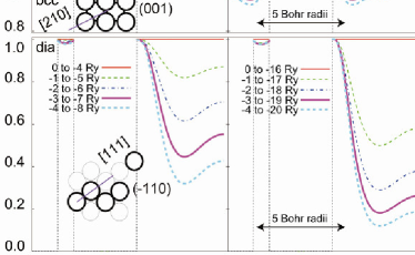
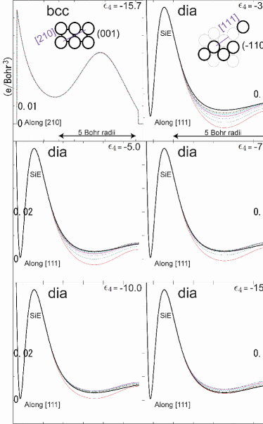
Like in Sect. VI.1, we use the examples of bcc and diamond-structured interstitials, and take $a=0.8t,$ $l_{\max}=4,$ and $N_{R}=51$ for bcc and $159$ for dia. We trace the interpolated function along the line from the centre of a sphere to that of the most distant nearest-neighbor void. For a crystal, this is the line from the centre of the Wigner-Seitz cell to its farthest corner, i.e. the [210] line for the bcc and the [111] line for the diamond structure. These paths leading deep into the respective interstitials are sketched in the insets of Fig. 4, which has bcc in the top- and dia in the bottom panels.

Fig. 4 now exhibits the interpolated functions for 10 different equidistant 4-point meshes, $\epsilon_{4}<\epsilon_{3}<\epsilon_{2}<\epsilon_{1},$ with $\epsilon_{1}$ stepping from 00 to $-4$ Ry ($\epsilon_{1}t^{2}$ from 0 to $-20)$ and $\epsilon_{4}$ stepping from $-4$ to $-8$ Ry ($\epsilon_{4}t^{2}$ from $-20$ to $-40)$ in the left-hand panel and from $-16$ to $-20$ Ry ($\epsilon_{4}t^{2}$ from $-80$ to $-100)$ in the right-hand panel. We notice, first of all, that the result is exact in all cases where $\epsilon_{1}=0$ (thin red full lines), as is expected. Secondly, all interpolated functions posses the required value $\left(=1\right)$ and first 3 derivatives $\left(=0\right)$ at the spheres. This is strictly true only when $\epsilon_{1}=0,$ but when $\epsilon_{1}\lesssim$ $-3$ Ry this does not hold along the part of the line where the spheres come close (see dia). The reason is that correct values and derivatives are only ensured for the angular-momentum averages over a sphere with $l\leq l_{\max},$ and not along a single direction (see also the discussion around eq. (32)).

Further into the interstitial, the interpolated functions are seen to deviate from $1,$ a deviation which increases not only with $\epsilon_{1}$ decreasing below zero, but also with the other energies decreasing below $\epsilon_{1}.$ As illustrated by comparison of the left- and right hand panels, the role of $\epsilon_{4}$ (the fastest decay) is to modify the behavior close to the spheres, given the first-, second-, and third radial derivatives. Further away from a sphere than $1/\sqrt{-\epsilon_{1}}$ and along the radial line far away from any other sphere, one might have expected the decay to be like that of the bare $s$-Hankel function with the longest range, i.e. like $\left(a/r\right)\exp\left\{-\left(r-a\right)\sqrt{-\epsilon_{1}}\right\}.$ However, the decays seen in the figure are more gradual. This is connected with the fact seen in Fig. 1, that the screened $s$-Hankel function, i.e. the $s$-USW, is a structure-adapted $s$-like wave which decays gradually towards the voids and steeply towards the neighboring spheres.

Most striking is the dramatic increase in the sensitivity to the mesh when going from the closely packed bcc- to the open diamond structure where the void and hard-sphere structures are identical and interpolation across the former is therefore difficult. Whereas interpolation of the function $\left|1\right\rangle$ can be seen to work for bcc as long as $-2\lesssim\epsilon_{1}\lesssim 0\,$Ry and $-6\,\mathrm{Ry}\lesssim\epsilon_{4}<\epsilon_{1},$ for diamond the requirement is something like: $-0.4\lesssim\epsilon_{1}\lesssim 0\,$Ry and $-1\lesssim\epsilon_{4}<\epsilon_{1};$ unless $\epsilon_{1}=0,$ in which case the interpolation is exact, regardless of the values of the other energies.


Refer to caption
Figure 4: (Color online) Interpolation of the function $\left|1\right\rangle$ across the bcc (top, note that the vertical scale starts at 0.8) and dia (bottom) interstitials using 10 different energy meshes. The results of these v&d interpolations are traced along the violet part of the [210] (bcc) and [111] (dia) lines indicated in the insets. $t=2.22$ Bohr radii, $a=0.8t,$ $l_{\max}=4,$ $N_{R}=51$ (bcc) and $159$ (dia). See Sect. VI.3.1.

VI.3.2 Charge densities of diamond-structured $sp^{3}$-bonded and ionic semiconductors from FP NMTO calculations

Fig. 5 illustrates a realistic example: The valence-electron density in diamond-structured Si. This charge density, here plotted in the $\left(110\right)$ plane through the $sp^{3}$ bonds, is the result of a density-functional calculation with the full-potential Nth-order MTO method 12Juelich ; 15FPNMTO . In this method, the density has the form:

$\displaystyle\rho\left(\mathbf{r}\right)=$ (104)
$\displaystyle\sum_{RL}\sum_{R^{\prime}L^{\prime}}\sum_{nn^{\prime}}\psi_{RL}^{\ast}\left(\epsilon_{n},\mathbf{r}_{R}\right)\Gamma_{nRL,n^{\prime}R^{\prime}L^{\prime}}\psi_{R^{\prime}L^{\prime}}\left(\epsilon_{n^{\prime}},\mathbf{r}_{R^{\prime}}\right)$
$\displaystyle+\sum_{R}\sum_{LL^{\prime}}Y_{RL}^{\ast}\left(\mathbf{\hat{r}}_{R}\right)Y_{RL^{\prime}}\left(\mathbf{\hat{r}}_{R}\right)\sum_{nn^{\prime}}\Gamma_{nRL,n^{\prime}R^{\prime}L^{\prime}}$
$\displaystyle\times\left[\varphi_{l}\left(\epsilon_{n},r_{R}\right)\varphi_{l^{\prime}}\left(\epsilon_{n^{\prime}},r_{R}\right)-\varphi_{l}^{o}\left(\epsilon_{n},r_{R}\right)\varphi_{l^{\prime}}^{o}\left(\epsilon_{n^{\prime}},r_{R}\right)\right]$

where $\epsilon_{n}$ are the energies chosen for solving Schrödinger’s equation; they spread far less that those used for the interpolation and include positive values. $\Gamma$ is the density matrix and $\psi$ is a screened spherical wave, basically a USW. $\varphi$ is not the potential from a v&d function like in Sect. IV.2, but a solution of the radial Scrödinger equation for the overlapping MT potential hardvsMT which defines the NMTO basis set, and $\varphi^{o}$ is the solution back-integrated over the MT zero, from the MT sphere to the hard sphere, inside which it is truncated. Hence, the function $\varphi\varphi-\varphi^{o}\varphi^{o}$ vanishes smoothly outside the MT sphere and jumps to $\varphi\varphi$ inside the hard sphere. This discontinuity is cancelled by the $\psi\Gamma\psi$ term in expression (104) which matches the $\varphi^{o}\varphi^{o}$ term and its first $2\mathrm{N}$ radial derivatives; here $\mathrm{N}$ is the order of the MTOs ($\mathrm{N=2}$ in the present calculations). The last term in (104) is a single-center sum over MT densities, each of which may be reduced to the simple warped-ASA form,86WASA $\sum_{L^{\prime\prime}}Y_{L^{\prime\prime}}\left(\mathbf{\hat{r}}\right)f_{L^{\prime\prime}}\left(r\right),$ for which Poisson’s equation is trivially solved. The $\psi\Gamma\psi$-term, however, is a complicated multi-centre sum occurring in all LCAO-like electronic-structure methods. This is the one we approximate by interpolation across the interstitial, matching to the $\varphi^{o}\varphi^{o}$ functions at the hard spheres when using the NMTO method. The result of this interpolation is shown in the middle panel of Fig. 5, while the right-hand panel shows the last term of expression (104), the MT part. The sum of the two is shown in the left-hand panel.

In the top row of Fig. 5, the voids in the diamond structure were filled with empty spheres such that the structure of the interstitial becomes bcc. The basis set for the electronic-structure calculation had MTOs on the two silicon as well as on the two empty spheres in the primitive cell and, hence, the density-functional calculation was one for 2(SiE).80Segall The same calculation delivered the input for the charge densities shown in the bottom row, but the E contributions were neglected, i.e. the $R$ sums in expression (104) were over the diamond rather than the bcc lattice. The bottom (dia) right-hand figure shows the density from the Si MTs, which is the same as in the top row. The density from the E MTs, present in the top (bcc) right-hand figure and missing in the bottom (dia) right-hand figure, is included in the bottom middle figure where it is taken into account by the interpolation across the dia interstitial matching to the $\varphi^{o}\varphi^{o}$ term at the Si hard spheres only. Adding the MT and interpolated contributions yields the charge densities shown in the left-hand panel. The ones in the top (bcc) and bottom (dia) rows are almost indistinguishable, but the densities deep in the diamond interstitial, below the lowest contour used in the figure (0.01 electrons/(Bohr radius)3), are not accurately interpolated, as we shall see in Fig. $\,7$.

We remark that the purpose of the above-mentioned construction of the Si charge density without empty spheres is to compare bcc and dia interpolations for the same Si input. Of course, we could have performed an entire selfconsistent FP NMTO calculation for Si without empty spheres 15FPNMTO .


Refer to caption
Figure 5: Valence charge density of diamond-structured Si resulting from a FP NMTO calculation for 2(SiE), plotted in the (110) plane through the $sp^{3}$ bonds. Like in eq. (104), the right-, middle, and left-hand panels show respectively the MT density, the $\psi\Gamma\psi$ density interpolated over the bcc (top) and dia (bottom) interstitials, and the sum of the two. The contours go from 0 to 0.3 in steps of 0.01 electrons per (Bohr radii)${}^{3}.$ The energy mesh was the same as in Figs 2 and 3, and the remaining parameters were like in Fig. 4. See Sect. VI.3.2.

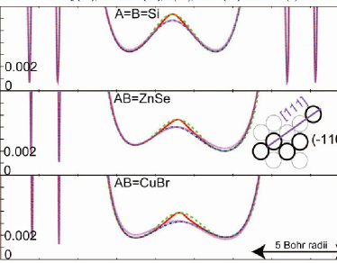
Quite a different charge density is that of the zinc-blende structured I-VII compound CuBr shown in Fig. 6. Rather than being covalent, it is ionic (Cu+Br${}^{-}=\,$Cu $3d^{10}$ Br $4p^{8})$ and has a full Cu 3$d$ shell. Despite this difference, the interstitial $\psi\Gamma\psi$ charge density, which is the one we interpolate, is not that different from the one in Si, albeit more concentrated around the atoms. The calculation leading to Fig. 6 was done exactly like the one leading to the top (bcc) row in Fig. 5 for Si. We shall return to CuBr in Sect. VII.


Refer to caption
Figure 6: As in the top (bcc) row of Fig. 5, but for zinc-blende structured CuBr calculated as CuBrEE’ with $a_{\mathrm{Cu}}\mathrm{=}a_{\mathrm{E}}\mathrm{=}1.72$ and $a_{\mathrm{Br}}\mathrm{=}a_{\mathrm{E}^{\prime}}\mathrm{=}2.00$ Bohr radii, whereby $t\mathrm{=}2.33$Bohr radii. See Sect. VI.3.2.

Like Fig. 4, but now for silicon, Fig. 7 shows charge densities along the open [210] and [111] directions in respectively the bcc and dia interstitials using different energy meshes for the interpolation. The upper figure to the left shows the $\psi\Gamma\psi$ density interpolated across the bcc interstitial, from a Si to an E sphere along $\left[210\right],$ using 6 different exponential 4-point meshes,

$$\epsilon_{n}=\epsilon_{1}\left(\epsilon_{4}/\epsilon_{1}\right)^{\left(n-1\right)/3},$$ (105)

with the highest energy: $\epsilon_{1}=-3.0,$ $-2.5,$ $-2.0,$ $-1.5,$ $-1.0,$ or $-0.5$ Ry and the lowest energy: $\epsilon_{4}=-15.7$ Ry. Only near the local maximum of the density where the $[210]$-line passes closely between a Si and an E sphere, deviations are detectable. The results for 24 other meshes with the same values of $\epsilon_{1}$, but with $\epsilon_{4}=-3.3,$ $-5.0,$ $-7.2,$ or $-10.0\,$Ry, deviate even less from each other, and have therefore not been shown. So for $sp^{3}$-bonded silicon, interpolation across the bcc interstitial is accurate and robust when using a 4-point mesh with energies distributed between $-16$ and $-2\,\mathrm{Ry.}$

In the remaining five parts of Fig. 7, the E spheres have been neglected and the interpolation is across the diamond-structured interstitial using the above-mentioned 30 different energy meshes. In this case, and like for the constant density in Fig. 4, the dependence on the energy mesh is strong. In order to be able to compare with the accurate result (solid black line) of the SiE calculation, we plot the total rather than the interpolated density. This we do along the violet [111] line, from slightly before the point inside a hard Si sphere where the density has fallen to a deep minimum and all densities are identical, then going into the interstitial, and finally ending at the midpoint between the two voids along $\left[111\right]$ (see also Fig. 5). Each of the five figures shows (in color) the density obtained using six different exponential energy meshes with the same $\epsilon_{4},$ and with $\epsilon_{1}$ running through the above-mentioned values.

We see that all total densities match with value and first 3 derivatives at the hard Si sphere, as they are designed to. But they deviate as we go deeper and deeper into the void. It seems that getting the correct 4th derivative requires $-20\lesssim\epsilon_{4}\lesssim-10$ Ry. In order to prevent the interpolated function from behaving too wildly deep in the interstitial, we must take the highest energy $\epsilon_{1}\lesssim-1$ Ry $\left(\epsilon_{1}t^{2}\lesssim-5\right)$. While acceptable interpolation is achieved with $-3.5\lesssim\epsilon_{1}\lesssim-2.5$ and $-5\lesssim\epsilon_{4}\lesssim-16$ Ry, the best is for the exponential mesh with $\epsilon_{1}=-3.0$ and $\epsilon_{4}=-15.7$ Ry (thick brown dot-dashed density in the bottom right-hand panel). This mesh actually reproduces the low densities in the voids better than does the one with $\epsilon_{1}=-1.54$ Ry and $\epsilon_{4}=-15.7$ Ry (thin blue dot-dashed density in the bottom right-hand panel) used for the charge-density contours in the bottom panel of Fig. 5. Of the 4 Si valence electrons, 1.19 are in the Si MT density and 2.81 are in the interstitial, and this is exactly what interpolation with the best mesh yields. The mesh with $\epsilon_{1}=-1.54$ Ry and the same $\epsilon_{4},$ giving an electron density along [111] about 0.002 electrons per (Bohr radius)3 higher in the void, yields 2.90 interstitial electrons, which is barely tolerable.

It is obvious from Fig. 7 that a 4-point mesh exists (the one with $\epsilon_{1}\sim-3.0$ Ry and $\epsilon_{4}\sim-15.7$) which makes the interpolation across the open interstitial almost perfect. Moreover, as long as one starts from a mesh with fixed $-20\lesssim\epsilon_{4}\lesssim-10$ Ry and $\epsilon_{4}<$ $\epsilon_{3}<$ $\epsilon_{2}\sim-5$ Ry, iterating merely the value of $\epsilon_{1}$ until the value of some additional constraint like the density at the centre of the void or the integral over the interstitial has the correct value, the interpolation will converge to this almost perfect density. However, iteration of $\epsilon_{1}$ is hardly practical because computation of the screened structure matrix (Sect.s VI.1 and VI.2) is the most expensive part of an interpolation. Moreover, this method is not a general one for treating additional constraints, so in the following section we shall devise a different scheme.


Refer to caption
Figure 7: (Color) As in Fig. 5, but plotted along the [210] line for the bcc- and along the [111] line for the diamond-structured interstitial, like in Fig. 4. The first figure shows the SiE $\psi\Gamma\psi$ density interpolated across the bcc interstitial, while the remaining figures show the total density for SiE (full black line) and for Si (broken, colored lines) with the $\psi\Gamma\psi$ part interpolated across the dia interstitial using 30 different exponential energy meshes. See Sect. VI.3.2 and eq. (105).

VII Extra constraints in open structures

Our examples of the closely-packed bcc- and the open diamond structures have clearly demonstrated (Fig.s 4 and 7) that whereas the energy mesh hardly matters for the former, whereby the interpolation across the narrow interstitial is robust, there is a strong dependence for the latter. This means that in order to interpolate across a bulky interstitial, more information is needed than the values and first three radial derivatives at its boundaries.

In density-functional calculations, one basic piece of information is the total number of valence electrons. It is fixed by the number of occupied bands (for metals, the occupied part of the Brillouin zone) and the density must integrate up to this number. Referring now to expression (104) and the corresponding figures 5 and 6 as examples, the MT density is trivial to integrate accurately, and subtracting this from the number of valence electrons gives what the integral over the interstitial of the interpolated density, should be; this is $\left\langle\varrho\right\rangle\mathcal{R}$ from eq.s (12), (8), and (97). For Si, this number was 2.81 electrons in the dia interstitial.

An often used option in MTO calculations is to fill the voids with E spheres whereby the interstitial becomes closely packed Stuttgart . This is what we did in the previous subsections to make the diamond structure bcc. The additional information provided herewith is the cubic-harmonic projections (11) at the E-spheres. For some structures, however, it takes numerous small spheres to fill the voids; melting silicon is one example, solid C60 another.

In such cases, it is more practical to evaluate the density at a few selected points, $\mathbf{r}_{c},$ deep in the interstitial and then constrain the interpolated density to those values. In LCAO-type calculations the evaluation is via the multi-centre expansion $\psi\left(\mathbf{r}_{c}\right)\Gamma\psi\left(\mathbf{r}_{c}\right),$ which is possible for a few points, but cumbersome for many.

An economic and general implementation of such extra constraints (on top of those $4N_{R}N_{L}$ constraints given by the matching at the hard spheres) amounts to computing the structure matrix at merely one extra energy and then with two different 4-point meshes generating two sets of v&d functions, a more localized set, $\varrho^{l}\left(\mathbf{r}\right),$ and a more extended one, $\varrho^{e}\left(\mathbf{r}\right).$ If, for instance, we use expression (105) to generate the five energies: $\epsilon_{5}<\epsilon_{4}<\epsilon_{3}<\epsilon_{2}<\epsilon_{1},$ then $\varrho^{l}\left(\mathbf{r}\right)$ and $\varrho^{e}\left(\mathbf{r}\right)$ are the sets obtained from respectively points $5$ to $2$ and points $4$ to $1.$ Any of the $4N_{R}N_{L}$ (see Sect. VI.2) weighted averages:

$$\varrho_{dRL}\left(\mathbf{r}\right)\equiv\varrho_{dRL}^{e}\left(\mathbf{r}\right)\alpha_{dRL}+\varrho_{dRL}^{l}\left(\mathbf{r}\right)\left(1-\alpha_{dRL}\right),$$ (106)

is seen to be a v-or-d function, and we now aim at determining the weights, $\alpha_{dRL},$ of the extended v&d functions such that the extra constraints are satisfied. Note that the number of extra constraints, $N_{c},$ cannot exceed $N_{R}N_{L}$, because only one extra USW set, e.g. $\psi_{RL}\left(\epsilon_{1},\mathbf{r}\right),$ has been added in the expansion (4) of $\rho\left(\mathbf{r}\right).$

Let the extra constraints be $q_{c}\left(\mathbf{r}\right),$ with $c$ going from 1 to $N_{c},$ and $q_{c}\equiv\left\langle q_{c}\mid\rho\right\rangle$ be the value of the $c$th constraint. As examples, the integral of the density in the interstitial is obtained with $q_{c}\left(\mathbf{r}\right)\equiv 1$ and the value at point $\mathbf{r}_{c}$ is obtained with $q_{c}\left(\mathbf{r}\right)\equiv\delta\left(\mathbf{r-r}_{c}\right).$ The estimate of the $c$th additional constraint is now:

$\displaystyle\sum_{dRL}\left\langle q_{c}|\varrho_{dRL}\right\rangle\mathcal{R}_{RL}^{\left(d\right)}=$
$\displaystyle\sum_{dRL}\left\langle q_{c}|\varrho_{dRL}^{e}-\varrho_{dRL}^{l}\right\rangle\mathcal{R}_{RL}^{\left(d\right)}\alpha_{dRL}+\sum_{dRL}\left\langle q_{c}|\varrho_{dRL}^{l}\right\rangle\mathcal{R}_{RL}^{\left(d\right)},$

as obtained by use of the interpolated density (8) and the v&d functions (106). Equating this estimate to the true value, $q_{c},$ of the constraint, leads to the linear equations:

$$\sum_{dRL}\left(q_{c,dRL}^{e}-q_{c,dRL}^{l}\right)\alpha_{dRL}=q_{c}-q_{c}^{l},$$ (107)

with $c$ going from $1$ to $N_{c},$ for the weights, $\alpha_{dRL}.$ On the right-hand side,

$$q_{c}^{l}\equiv\sum_{dRL}q_{c,dRL}^{l}$$

is the estimate of the constraint using localized density:

$$\rho^{l}\left(\mathbf{r}\right)=\sum_{dRL}\varrho_{dRL}^{l}\left(\mathbf{r}\right)\mathcal{R}_{RL}^{\left(d\right)},$$

while $q_{c,dRL}^{l}\equiv\left\langle q_{c}|\varrho_{dRL}^{l}\right\rangle\mathcal{R}_{RL}^{\left(d\right)}$ is its $dRL$ component. Similarly for $q_{c,dRL}^{e}.$ Since the number, $4N_{L}N_{R},$ of unknown weights exceeds the number, $N_{c},$ of extra constraints, we avoid unphysical solutions of equations (107) by requiring that the weights, $\alpha_{dRL},$ of the extended v&d functions be small. Specifically, we minimize the sum of the square weights, $\sum_{dRl}\alpha_{dRL}^{2},$ subject to the constraints (107). This leads to the $4N_{R}N_{L}$ Lagrangian equations:

$$\frac{\partial}{\partial\alpha_{d^{\prime}R^{\prime}L^{\prime}}}\sum_{dRL}\left\{\alpha_{dRL}^{2}-\sum_{c=1}^{N_{c}}\lambda_{c}\left(q_{c,dRL}^{e}-q_{c,dRL}^{l}\right)\alpha_{dRL}\right\}=0,$$

for $d\mathrm{=}1$ to $4,\;R\mathrm{=}1$ to $N_{R},$ and$\;L\mathrm{=}1$ to $N_{L}\left(R\right),$ or explicitly:

$$\alpha_{dRL}=\sum_{c=1}^{N_{c}}\frac{1}{2}\lambda_{c}\left(q_{c,dRL}^{e}-q_{c,dRL}^{l}\right),$$ (108)

to be solved together with eq.s (107) for the weights, $\alpha_{dRL},$ and the Langrangian multipliers, $\lambda_{c}.$ Insertion of (108) in eq. (107) yields the $N_{c}$ linear equations for the $N_{c}$ Langrangian multipliers:

$\displaystyle\sum_{c^{\prime}}\frac{1}{2}\lambda_{c^{\prime}}\sum_{dRL}\left(q_{c^{\prime},dRL}^{e}-q_{c^{\prime},dRL}^{l}\right)\left(q_{c,dRL}^{e}-q_{c,dRL}^{l}\right)$
$\displaystyle=q_{c}-q_{c}^{l},$ (109)

for $c\mathrm{=}1$ to $N_{c},$ which may be solved and inserted in eq. (108) to yield the weights.

The Coulomb potential from the constrained v&d functions (106) is of course given by the same weighted average of the potentials $\varphi_{dRL}^{e}\left(\mathbf{r}\right)$ and $\varphi_{dRL}^{l}\left(\mathbf{r}\right),$ where the latter are those of the charge densities $\varrho_{dRL}^{e}\left(\mathbf{r}\right)$ and $\varrho_{dRL}^{l}\left(\mathbf{r}\right),$ obtained as described in Sect. IV.2.

In Fig. 8 we demonstrate how well this works for the valence electron densities in diamond-structured Si (top) where $N_{R}N_{L}\mathrm{=}4$, and in the zinc-blende structured II-VI and I-VII compounds, ZnSe (middle) and CuBr (bottom) where $N_{R}N_{L}\mathrm{=}8$. For all three materials, we used the five energies, $\epsilon_{5}$ to $\epsilon_{1},$ obtained with the same 10percent exponential mesh: $\epsilon_{n}=-4\left(4\right)^{\left(n-2\right)/3}\,\mathrm{Ry.}$ Fig. 8 shows densities along the open [111] direction, but now all the way across the dia interstitial, because with the A and B atoms different, the density is not symmetric around any of their midpoints as in Fig. $\,7$. The aim is to interpolate the density across the dia interstitial as in the bottom part of Fig. 5, i.e. without using the v&d information computed at the empty sphere(s), but obtaining also the densities below 0.01 electrons per (Bohr radii)3 accurately by installing the following constraints: The total number of electrons be 8 and 18 electrons per cell for respectively Si and the compound semiconductors $(N_{c}\mathrm{=}1),$ also the density at the centre(s) of the void(s) be correct ($N_{c}\mathrm{=}2$ for Si and $3$ for the compounds), and also the density between the voids be correct ($N_{c}\mathrm{=}3$ and $4)$.

This scheme is seen to work very well, indeed.


Refer to caption
Figure 8: (Color online) Total densities plotted along the [111] line shown in the inset across the dia interstitial for Si (top), ZnSe (middle), and CuBr (bottom). This line crosses the BE’EA spheres from left to right, i.e. the anion is to the left and the cation to the right. For each material, the full red line shows the density calculated as ABEE’, i.e. the interpolation was merely over the bcc interstitial, while in the three other curves, the interpolation was across the dia interstitial and constrained. The dotted magenta curve results from constraining merely the integral over the interstitial. In the dot-dashed blue curve also the densities at center(s) of the void(s), i.e. the minima, were constrained. In the dashed green curve, finally, also the density between the voids, i.e. near the relative maximum, was constrained. We used the energies: $\epsilon_{n}=-4\left(4\right)^{\left(n-2\right)/3}\,\mathrm{Ry}$ with $n\mathrm{=}1$ to 5, i.e. $-16,$ $-10.1,$ $-6.3,$ $-4,$ and $-2.5$ Ry. The screening of the dia structure matrix required $N_{R}\mathrm{=}87$ sites and $l_{\max}\mathrm{=}4$. See also Figs. 5, 6, and 7, as well as Sect. VII.

VIII Conclusions

We have carried through the program laid out in the Introduction and have derived a formalism for numerical 3D interpolation across a hard-sphere interstitial from the cubic-harmonic projections of the target function, $\rho\left(\mathbf{r}\right),$ and its first 3 radial derivatives at the spheres. Whereas this knowledge suffices for closely-packed structures, additional information such as the integral of $\rho\left(\mathbf{r}\right)$ over the interstitial and/or the values at specific points deep inside the interstitial is needed for open structures. This was illustrated by application to a constant function and to the valence charge densities in Si, ZnSe, and CuBr, interpolated across either the bcc- or the zinc-blende-structured interstitial, depending on whether or not the voids were filled with empty spheres (Figs 4-7).

Our interpolation is based on localized, structure-adapted sets of spherical-waves (USWs), $\psi_{RL}\left(\epsilon_{n},\mathbf{r}\right),$ with 4 different energies (Fig. 1). These set are combined linearly into sets of so-called value-and-derivative (v&d) functions, $\varrho_{dRL}\left(\mathbf{r}\right)$ with $d\mathrm{=}0$ to 3, confined essentially to the Voronoi cells (top row in Fig.s 2 and 3). The formalism is expressed in terms of energy-divided differences of the USWs and their slope matrix with elements $S_{RL,R^{\prime}L^{\prime}}\left(\epsilon_{n}\right)$ (Sect.s II and III). For the bcc structure, accurate results were obtained with an exponential energy mesh spanned by $\epsilon_{4}\mathrm{=}-80/t^{2}$ and $\epsilon_{1}\mathrm{=}-12/t^{2},$ where $t$ is the average radius of touching spheres and gives the scale of the structure. We expect this mesh to be satisfactory for all closely-packed structures. The extra constraints needed for open structures require the use of an extra energy and we demonstrated that the exponential 5-point mesh with the same limits, $\epsilon_{5}t^{2}\mathrm{=}-80$ and $\epsilon_{1}t^{2}\mathrm{=}-12,$ gives excellent results for the zincblende structure (Fig. 8).

Solving Poisson’s equation for the interpolated function requires the solutions $\psi_{RL}\left(\epsilon_{0}\mathcal{\equiv}0,\mathbf{r}\right)$ of the Laplace equation as well. The localized potentials (middle row in Fig.s 2 and 3) for the v&d functions are expressed in terms of energy-divided differences one order higher than for the v&d functions. The multipoles needed in order to make the localized potential regular (bottom row in Fig.s 2 and 3), are given by the same differences of the slope matrix (Sect. IV). The latter also give the integrals over the interstitial (Sect. V).

The slope matrix is screened through inversion of the analytical, bare structure matrix for a cluster with $N_{R}$ sites surrounding sites. We found $N_{R}\mathrm{\sim}60$ for closely packed structures and 2-3 times larger for open 3D structures like zincblende (Sect. VI.1). For a given site, $R,$ only those $L$-channels must be kept for which the target function does not vanish due to symmetry. If the local point symmetry is high, the number, $N_{L}\left(R\right),$ of $L$-channels is considerably smaller than the maximum, $\left(1+l_{\max}\right)^{2}\sim 25,$ for instance $4-5$ for tetrahedral symmetry. The dimension of the matrix to be inverted is thus $\sum_{R}^{N_{R}}N_{L}\left(R\right).$ For interpolating a function without symmetry this can be large $\left(10^{3}-10^{4}\right),$ but the process increases only linearly with the number of sites. Whereas $N_{R}\mathrm{\sim}100$ is needed in the screening calculation, all subsequent matrix operations, i.e. those needed to form v&d functions, potentials, and integrals, can in case of space-group symmetry and for interpolating the charge density be performed with a symmetrized slope matrix in which equivalent sites have been summed over so that $N_{R}$ is merely the number of inequivalent sites. Hence, $N_{R}\mathrm{=}2$ for the zinc-blende structure (Sect. VI.2).

This method was developed for interpolating charge densities and is currently used for density-functional FP-NMTO calculations 15FPNMTO ; 15LiPB . Since it is generally applicable, local, and based on cubic harmonics, we expect it to find numerous uses.

IX Acknowledgements

We are grateful to Dr. M. Höppner for testing our codes, for providing valuable feedback, and for help with writing the manual. Prof. H. Takagi is acknowledged for support and Dr. A. Schnyder for providing many useful examples.

X Appendix: One-center cubic-harmonic expansions

X.1 $RL$-projections of the v&d functions

The expressions derived in Sect. III for the short-ranged v&d functions as linear combinations of USWs are particularly useful for solving Poisson’s equation and for computing integrals over the interstitial as was done in Sect.s IV and V, respectively. For other purposes, cubic-harmonic expansions like (73) around single centers may be more practical. The coefficients are the projections, $\mathcal{\hat{P}}_{R^{\prime}L^{\prime}}\left(r\right)\varrho_{dRL}\left(\mathbf{r}\right),$ given in eq. (14) to third order in the distance from the spheres, and beyond this, by the expresssions derived below. These higher-order terms are responsible for the sensitivity to the energy mesh displayed in Fig. 7.

The expressions for $\mathcal{\hat{P}}_{R^{\prime}L^{\prime}}\left(r\right)\varrho_{dRL}\left(\mathbf{r}\right)$ might be obtained by projecting the USWs $\psi_{RL}\left(\epsilon_{n},\mathbf{r}\right)$ in the first eq. (63) by means of (16), but it is simpler to commute $RL$-projection with taking $\varepsilon$-divided differences. Like in (51), we thus start by taking the $\varepsilon$-divided differences of the projection using the binomial rule (50). In order that the result clearly exhibit the parts leading to eq. (14), we use $u\left(\varepsilon,r\right)\equiv f\left(\varepsilon,r\right)-g\left(\varepsilon,r\right)$ instead of $f\left(\varepsilon,r\right)$ and, expression (37) divided by $r$ instead of (16). The result is:

$\displaystyle\mathcal{\hat{P}}\left(r\right)\psi_{1}\left(\mathbf{r}\right)$ $\displaystyle=u_{1}\left(r\right)+g_{1}\left(r\right)\mathcal{S}_{1},$
$\displaystyle\mathcal{\hat{P}}\left(r\right)\psi_{12}\left(\mathbf{r}\right)$ $\displaystyle=u_{12}\left(r\right)+g_{1}\left(r\right)S_{12}+g_{12}\left(r\right)\mathcal{S}_{2},$
$\displaystyle\mathcal{\hat{P}}\left(r\right)\psi_{123}\left(\mathbf{r}\right)$ $\displaystyle=u_{123}\left(r\right)+g_{1}\left(r\right)S_{123}+g_{12}\left(r\right)S_{23}$
$\displaystyle+g_{123}\left(r\right)\mathcal{S}_{3},$
$\displaystyle\mathcal{\hat{P}}\left(r\right)\psi_{1234}\left(\mathbf{r}\right)$ $\displaystyle=u_{1234}\left(r\right)+g_{1}\left(r\right)S_{1234}+g_{12}\left(r\right)S_{234}$
$\displaystyle+g_{123}\left(r\right)S_{34}+g_{1234}\left(r\right)\mathcal{S}_{4}.$ (110)

The terms present in (110) and not in eq.s (51) are of order higher than 3rd in $r-a.$

The projections of the set of 3rd-derivative functions (53) are then:

$\displaystyle\mathcal{\hat{P}}\left(r\right)\varrho_{3}\left(\mathbf{r}\right)$
$\displaystyle=\mathcal{\hat{P}}\left(r\right)\psi_{123}\left(\mathbf{r}\right)D_{3,3}+\mathcal{\hat{P}}\left(r\right)\psi_{1234}\left(\mathbf{r}\right)D_{4,3}$
$\displaystyle=-g_{12}\left(r\right)+u_{123}\left(r\right)D_{3,3}$
$\displaystyle+g_{123}\left(r\right)\left[\mathcal{S}_{3}D_{3,3}+S_{34}D_{4,3}\right]$
$\displaystyle+u_{1234}\left(r\right)D_{4,3}+g_{1234}\left(r\right)\mathcal{S}_{4}D_{4,3}.$ (111)

By construction, the coefficient to $g_{1}\left(r\right)$ vanishes and the coefficient to $g_{12}\left(r\right)$ is

$$S_{23}D_{3,3}+S_{234}D_{4,3}=-1.$$

With eq.s (44)-(49) in mind, we realize that the terms after the diagonal term, $-g_{12}\left(r\right),$ in (111) are smaller than $\left(r-a\right)^{3}.$

The projections of the set of 1st-derivative functions (63)-(64) are:

$\displaystyle\mathcal{\hat{P}}\left(r\right)\varrho_{1}\left(\mathbf{r}\right)$
$\displaystyle=\mathcal{\hat{P}}\left(r\right)\psi_{123}\left(\mathbf{r}\right)D_{3,1}+\mathcal{\hat{P}}\left(r\right)\psi_{1234}\left(\mathbf{r}\right)D_{4,1}$
$\displaystyle=g_{1}\left(r\right)-g_{12}\left(r\right)\left(\epsilon_{1}-w\right)+u_{123}\left(r\right)D_{3,1}$
$\displaystyle+g_{123}\left(r\right)\left[\mathcal{S}_{3}D_{3,1}+S_{34}D_{4,1}\right]$
$\displaystyle+u_{1234}\left(r\right)D_{4,1}+g_{1234}\left(r\right)\mathcal{S}_{4}D_{4,1},$ (112)

where the coefficient to $g_{1}\left(r\right)$ is:

$$S_{123}D_{3,1}+S_{1234}D_{4,1}=1,$$

and that to $g_{12}\left(r\right)$ is:

$$S_{23}D_{3,1}+S_{234}D_{4,1}=-\left(\epsilon_{1}-w\right).$$

The first, diagonal $g_{1}\left(r\right)$-term gives the 1st derivative, and its contribution to the 3rd derivative is cancelled by the second term, $-g_{12}\left(r\right)\left(\epsilon_{1}-w\right)$.

The projections of the set of 2nd-derivative functions (63)-(72) are:

$\displaystyle\mathcal{\hat{P}}\left(r\right)\varrho_{2}\left(\mathbf{r}\right)a$
$\displaystyle=-\mathcal{\hat{P}}\left(r\right)\psi_{12}\left(\mathbf{r}\right)$
$\displaystyle+\mathcal{\hat{P}}\left(r\right)\psi_{123}\left(\mathbf{r}\right)D_{3,2}a+\mathcal{\hat{P}}\left(r\right)\psi_{1234}\left(\mathbf{r}\right)D_{4,2}a$
$\displaystyle=-u_{12}\left(r\right)+u_{123}\left(r\right)D_{3,2}a$
$\displaystyle+g_{123}\left(r\right)\left[S_{34}D_{4,2}+\mathcal{S}_{3}D_{3,2}\right]a$
$\displaystyle+u_{1234}\left(r\right)D_{4,2}a+g_{1234}\left(r\right)\mathcal{S}_{4}D_{4,2}a,$ (113)

where the coefficients:

$$-S_{12}+S_{123}D_{3,2}a+S_{1234}D_{4,2}a,$$

and:

$$-\mathcal{S}_{2}+S_{23}D_{3,2}a+S_{234}D_{4,2}a,$$

to respectively $g_{1}\left(r\right)$ and $g_{12}\left(r\right)$ vanish. From eq. (45) it follows that $-u_{12}\left(r\right)=\frac{a}{r}\frac{\left(r-a\right)^{2}}{2!}+\,o,$ which is the behavior of $\mathcal{\hat{P}}\left(r\right)\varrho_{2}\left(\mathbf{r}\right)a$ specified by eq. (14).

The projections of the set of value functions (63)-(72) are:

$\displaystyle\mathcal{\hat{P}}\left(r\right)\rho_{0}\left(\mathbf{r}\right)a$
$\displaystyle=\mathcal{\hat{P}}\left(r\right)\psi_{1}\left(\mathbf{r}\right)-\mathcal{\hat{P}}\left(r\right)\psi_{12}\left(\mathbf{r}\right)\left(\epsilon_{1}-w\right)$
$\displaystyle+\mathcal{\hat{P}}\left(r\right)\psi_{123}\left(\mathbf{r}\right)D_{3,0}a+\mathcal{\hat{P}}\left(r\right)\psi_{1234}\left(\mathbf{r}\right)D_{4,0}a$
$\displaystyle=u_{1}\left(r\right)-u_{12}\left(r\right)\left(\epsilon_{1}-w\right)+g_{12}\left(r\right)aw^{\prime}$
$\displaystyle+u_{123}\left(r\right)D_{3,0}a+g_{123}\left(r\right)\left(\mathcal{S}_{3}D_{3,0}+S_{34}D_{4,0}\right)a$
$\displaystyle+u_{1234}\left(r\right)D_{4,0}a-g_{1234}\left(r\right)\mathcal{S}_{4}D_{4,0}a.$ (114)

Here, the coefficient,

$$\mathcal{S}_{1}-S_{12}\left(\epsilon_{1}-w\right)+S_{123}D_{3,0}a+S_{1234}D_{4,0}a,$$

to $g_{1}\left(r\right)$ has vanished and the coefficient to $g_{12}\left(r\right)$ has worked out to:

$$-\mathcal{S}_{2}\left(\epsilon_{1}-w\right)+S_{23}D_{3,0}a+S_{234}D_{4,0}a=aw^{\prime}.$$

In (114) then, the $u_{1}\left(r\right)$-term gives the value, and the parts of this term which behave as $\left(r-a\right)^{2}$ and $\left(r-a\right)^{3}$ are cancelled by respectively $-u_{12}\left(r\right)\left(\epsilon_{1}-w\right)$ and $g_{12}\left(r\right)aw^{\prime}.$

The radial functions $u_{Rl}\left(\varepsilon,r\right)$ and $g_{Rl}\left(\varepsilon,r\right)$ may be generated by numerical integration outwards from the boundary conditions: $u_{Rl}\left(\varepsilon,a_{R}\right)=1,$ $u_{Rl}^{\prime}\left(\varepsilon,a_{R}\right)=-1/a_{R},$ and (18). Alternatively, these functions may be expressed in terms of the spherical Neumann and Bessel functions using eq.s (28) and (21).

As said after eq. (73), the one-center cubic-harmonics expansions with the radial functions $\mathcal{\hat{P}}_{R^{\prime}L^{\prime}}\left(r\right)\varrho_{dRL}\left(\mathbf{r}\right)$ are valid at and outside the $R^{\prime}$-sphere and inside the sphere touching the nearest-neighbor sphere. Inside the $R^{\prime}$-sphere, all v&d functions vanish.

X.2 $RL$-projections of the localized potentials from v&d functions

Here we shall derive the radial functions in the $L^{\prime}$-expansion (10) around the arbitrary site $R^{\prime}$ of the localized potential (89) from the v&d function, $\varrho_{dRL}.$ Examples of the localized and regular potentials were shown in respectively the middle and bottom rows of Fig.s 2 and 3, and were discussed in Sect. IV.2. The regular potentials look very smooth so that their one-center expansions should converge well. But this smooth behavior is due to domination by the central point-charge potential which gives long range, and thus complicates the summation $\sum_{R}\mathcal{\hat{P}}_{R^{\prime}L^{\prime}}\left(r\right)\varphi_{dRL}\left(\mathbf{r}\right)\mathcal{R}_{RL}^{\left(d\right)}$ for the projection of $V\left(\mathbf{r}\right)$, and will in any case be modified (usually reduced) when adding the potentials from the remaining charges in the system. It is therefore better, at the end of the $V\left(\mathbf{r}\right)$-calculation, to sum up all multipole moments at the various sites, $R^{\prime\prime},$ and then expand their potentials around the site, $R^{\prime},$ in question, using the well-known expression (eq.$\,($23), $\varepsilon\mathrm{=}0)$ with its large radius of convergence, $d_{R^{\prime\prime}R^{\prime}}.$ Below, we shall therefore only consider the localized potential.

The $d$th energy-divided difference, $\psi_{1..d+1;RL}\left(\mathbf{r}\right),$ of a USW gives rise to the localized potential, $\phi_{1..d+1;RL}^{loc}\left(\mathbf{r}\right),$ given by eq. (78). Its cubic-harmonic expansion (79) around the arbitrary site $\mathbf{R}^{\prime}$ has coefficients, which are $8\pi$ times the projections given by expressions (80).

Since the v&d functions are superpositions (63)-(72) of energy-divided differences of USWs: $\varrho_{d}\left(\mathbf{r}\right)=\sum_{n}\psi_{1..n}\left(\mathbf{r}\right)D_{n,d},$ the potentials from $\varrho_{d}\left(\mathbf{r}\right)$ are the same superpositions of the potentials, $\phi_{1..n}^{loc}\left(\mathbf{r}\right),$ from $\psi_{1..n}\left(\mathbf{r}\right)$:

$$\varphi_{d}^{loc}\left(\mathbf{r}\right)=\sum\nolimits_{n}\phi_{1..n}^{loc}\left(\mathbf{r}\right)D_{n,d}=8\pi\sum\nolimits_{n}\psi_{0...n}\left(\mathbf{r}\right)D_{n,d}\,,$$

and similarly for the projections of the v&d functions and of their potentials:

$\displaystyle\mathcal{\hat{P}}\left(r\right)\varrho_{d}\left(\mathbf{r}\right)$ $\displaystyle=\sum_{n=1}^{4}\mathcal{\hat{P}}\left(r\right)\psi_{1..n}\left(\mathbf{r}\right)D_{n,d}\,,\;\;\mathrm{and}$
$\displaystyle\mathcal{\hat{P}}\left(r\right)\varphi_{d}^{loc}\left(\mathbf{r}\right)$ $\displaystyle=8\pi\sum_{n=1}^{4}\mathcal{\hat{P}}\left(r\right)\psi_{0...n}\left(\mathbf{r}\right)D_{n,d}\,.$

Comparison of $\mathcal{\hat{P}}\left(r\right)\psi_{1..n}\left(\mathbf{r}\right)$ in (110) with $\mathcal{\hat{P}}\left(r\right)\psi_{0...n}\left(\mathbf{r}\right)$ in (80) now shows that expressions (111)-(114) for $\mathcal{\hat{P}}\left(r\right)\varrho_{d}\left(\mathbf{r}\right)$ hold also for $\mathcal{\hat{P}}\left(r\right)\varphi_{d}^{loc}\left(\mathbf{r}\right)/8\pi,$ provided that (1) in all energy-divided-difference functions of $\mathbf{r}$ and $r$ – but not in the coefficients – the subscripts $1..n$ are substituted by $0...n$ and (2) the term $g_{0}\left(r\right)\sum_{n=1}^{4}S_{0...n}D_{n,d}$ is added. (1) is as if Poisson’s equation had been solved by taking the energy-divided differences of only the radial functions, but not of the slope matrix, and (2) is the Laplace term giving the multipole potential when continued inside the $R^{\prime}$-sphere (see eq. (81)). With the localized potential from the value function as an example, we get, starting from eq. (114):

$\displaystyle\frac{1}{8\pi}\mathcal{\hat{P}}\left(r\right)\varphi_{0}^{loc}\left(\mathbf{r}\right)a$
$\displaystyle=g_{0}\left(r\right)\sum\nolimits_{n=1}^{4}S_{0...n}D_{n,0}$
$\displaystyle+u_{01}\left(r\right)-u_{012}\left(r\right)\left(\epsilon_{1}-w\right)+g_{012}\left(r\right)aw^{\prime}$
$\displaystyle+u_{0123}\left(r\right)D_{3,0}a+g_{0123}\left(r\right)\left(\mathcal{S}_{3}D_{3,0}+S_{34}D_{4,0}\right)a$
$\displaystyle+u_{01234}\left(r\right)D_{4,0}a-g_{01234}\left(r\right)\mathcal{S}_{4}D_{4,0}a.$ (115)

The expansion (10) around $\mathbf{R}^{\prime}$ holds also inside the sphere, i.e. for $0\leq r\leq\min_{R^{\prime\prime}}\left(d_{R^{\prime\prime}R^{\prime}}-a_{R^{\prime}}\right),$ provided that we keep only the Laplace term, $g_{0}\left(r\right)\sum S_{0...n}D_{n,d},$ there. Without this term, the radial potential from the value function (115) increases smoothly from zero inside the sphere to $u_{01}\left(r\right)+o=-\frac{a}{r}\frac{\left(r-a\right)^{2}}{2!}+o$ outside. Here $o$ is given by eq. (13). The analogous potential from the 1st derivative function, increases outside as $g_{01}+o=-\frac{1}{r}\frac{\left(r-a\right)^{3}}{3!}+\,o,$ and those from the 2nd and 3rd derivative functions as $o.$

These projections with $L^{\prime}\mathrm{=}0$ are used to construct the overlapping MT potential 98MRS ; 09OMTA defining the 3rd generation LMTO 94Trieste ; 98MRS ; 00Rashmi and NMTO 00NMTO ; 00Odile ; 12Juelich ; 15FPNMTO basis sets.


References

  • (1) R.M. Martin, Electronic Structure: Basic Theory and Practical Methods, Cambridge University Press, 2008
  • (2) R.M. Martin, K. Terakura, I. Terakura, and Y. Zenpo, “Busshitsu no denshi jotai 1-2” in Springer University Textbooks (Maruzen, Tokyo, 2012).
  • (3) Electronic Structure and Physical Properties of Solids. The Uses of the LMTO Method, ed. H. Dreyssé. Springer Berlin/Heidelberg (2000) [Springer Lecture notes in Physics, vol. 535].
  • (4) K.H. Weyrich, Solid State Commun. 54, 975 (1985).
  • (5) S.Y. Savrasov, Phys. Rev. B 54, 16470 (1996).
  • (6) J.M. Wills, O. Eriksson, M. Alouani, and D.L. Price in Ref. 00Dreysse
  • (7) M. Methfessel, M. van Schilfgaarde, and R.A. Casali in Ref. 00Dreysse .
  • (8) T. Kotani and M. van Schilfgaarde, Phys. Rev. B 81, 125117 (2010).
  • (9) Lectures on Methods of Electronic Structure Calculations, Eds.: V. Kumar, O.K. Andersen, A. Mookerjee, World Sci. Publ.Co., Singapore (1994)
  • (10) O.K. Andersen, O. Jepsen, and G. Krier in Ref. 94lectures .
  • (11) In the 3rd generation LMTO 94Trieste ; 98MRS and NMTO 00NMTO ; 00Odile ; 00Rashmi ; 12Juelich ; 15FPNMTO band-structure methods both hard spheres and MT spheres are used. The former are those of the present paper and the latter are for presenting the MT part of the potential. The hard and the MT spheres are concentric with the respective radii $a$ and $s>a.$ A MT sphere can overlap neighboring MT spheres, but not hard spheres.
  • (12) D.R. Bowler and T. Miyazaki, Rep. Prog. Phys. 75, 036503 (2012)
  • (13) O.K. Andersen and R.G. Wooley, Molecular Physics 26, 905-927 (1973).
  • (14) N. Stefanou and R. Zeller, J. Phys.: Condens. Matter 3, 7599 (1991).
  • (15) J. Kollár, L.Vitos, and H.L. Skriver in Ref. 00Dreysse .
  • (16) O.K. Andersen, Solid State Commun. 13, 133-136 (1973).
  • (17) O.K. Andersen, Phys. Rev. B 12, 3060 (1975).
  • (18) D. Glötzel, B. Segall, and O.K. Andersen, Solid State Commun. 36, 403 (1980).
  • (19) O. Gunnarsson, O. Jepsen, and O.K. Andersen, Phys. Rev. B 27, 7144 (1983).
  • (20) H.L. Skriver The LMTO Method (Springer Verlag, Berlin, 1984).
  • (21) W.R.L. Lambrecht and O.K. Andersen, Surface Science 178, 256-263 (1986).
  • (22) H.L. Skriver and N.M. Rosengaard, Phys. Rev. B 43, 9538 (1991); .N.M. Rosengaard and H.L. Skriver, Phys. Rev. 50, 4848 (1994).
  • (23) M. van Schilfgaarde and F. Herman, Phys. Rev. Lett. 71, 1923 (1993).
  • (24) S. Frota-Pessoa, Phys. Rev. B 36, 904 (1987); P. R. Peduto, S. Frota-Pessoa, and M. S. Methfessel, Phys, Rev. B 44, 13283 (1991).
  • (25) H.J. Nowak, O.K. Andersen, T. Fujiwara, O. Jepsen and P. Vargas, Phys. Rev. B 44, 3577 (1991).
  • (26) S.K. Bose, O. Jepsen, and O.K. Andersen, Phys. Rev. B 48, 4265 (1993).
  • (27) P. Vargas in Ref. 94lectures .
  • (28) T. Saha, I. Dasgupta, and A. Mookerjee, J. Phys.: Condens. Matter 6, L245 (1994).
  • (29) I. A. Abrikosov and H. L. Skriver, Phys. Rev. B 47, 16532 (1993).
  • (30) A. V. Ruban, I. A. Abrikosov, D. Ya. Kats, D. Gorelikov, K. W. Jacobsen, and H. L. Skriver, Phys. Rev. B 49, 11383 (1994).
  • (31) I. Turek, V. Drchal, J. Kudrnovsky, M. Sob, and P. Weinberger, Electronic Structure of Disordered Alloys, Surfaces, and Interfaces (Kluwer Academic Publishers, Boston/London/Dordrecht, 1997).
  • (32) P. Weinberger, I. Turek, and L. Szunyogh, Int. J. Quant. Chem. 63, 165 (1997).
  • (33) “The Stuttgart TB-LMTO-ASA Code.” 
  • (34) O.K. Andersen, T. Saha-Dasgupta, R.W. Tank, C. Arcangeli, O. Jepsen, G. Krier in Ref. 00Dreysse , Appendix.
  • (35) O.K. Andersen, C. Arcangeli, R.W. Tank, T. Saha-Dasgupta, G. Krier, O. Jepsen, I. Dasgupta in: Tight-Binding Approach to Computational Materials Science, eds. L. Colombo, A. Gonis, P. Turchi. MRS Symposium Proceedings Series, vol 491 (1998).
  • (36) M. Zwierzycki and O.K. Andersen, Acta Physica Polonica A 115, 64 (2009).
  • (37) R.W. Tank and C. Arcangeli, phys. stat. sol. 217, 89 (2000).
  • (38) O.K. Andersen and T. Saha-Dasgupta, Phys. Rev. B 62, R16219 (2000).
  • (39) O.K. Andersen, T. Saha-Dasgupta, R.W. Tank, C. Arcangeli, O. Jepsen, G. Krier in Ref. 00Dreysse .
  • (40) O.K. Andersen, in: Correlated Electrons: From Models to Materials, Eds. E. Pavarini, E. Koch, F. Anders, and M. Jarrell, Forschungzentrum Jülich, Reihe Modelling and Simulation Vol. 2, Jülich, 2012, ISBN 978-3-89336-796-2.
  • (41) Y. Nohara and O.K. Andersen, unpublished.
  • (42) M. Methfessel, Phys. Rev. B 38, 1537 (1988).
  • (43) M. Methfessel, C.O. Rodriguez, and O.K. Andersen, Phys. Rev. B 40, 2009 (1989).
  • (44) A. Svane and O.K. Andersen, Phys. Rev. B 34, 5512 (1986)
  • (45) M. Springborg and O.K. Andersen, J. Chem. Phys. 87, 7125 (1986).
  • (46) Y. Nohara, O.K. Andersen, M. Haverkort, L. Dudy, J.W. Allen, J.D. Denlinger, unpublished.
  • (47) We complex conjugate $Y_{L}\left(\mathbf{\hat{r}}\right)$ as appropriate had it been a complex spherical harmonic rather than a real cubic harmonic because this makes the formalism more general.
  • (48) J. Korringa, Physica 13, 392 (1947); W. Kohn and J. Rostoker, Phys. Rev. 94, 1111 (1954).
  • (49) F.S. Ham and B. Segal, Phys. Rev. 124, 1786 (1961).
  • (50) Our bare structure matrix is $\kappa^{l+l^{\prime}}$ times the one with the usual definition.
  • (51) O.K. Andersen and O. Jepsen, Phys. Rev. Lett. 53, 2571 (1984); only $\varepsilon=0$ was used.
  • (52) O.K. Andersen, A.V. Postnikov, and S. Yu. Savrasov, in Applications of Multiple Scattering Theory to Materials Science, eds. W.H. Butler, P.H. Dederichs, A. Gonis, and R.L. Weaver, MRS Symposia Proceedings No. 253 (Materials Research Society, Pittsburgh, 1992) pp 37-70.
  • (53) R. Zeller, P.H. Dederichs, B. Ujfalussy, L. Szunyogh, P. Weinberger, Phys. Rev. B 52, 8807 (1995).
  • (54) USWs with higher energies and lower $l_{\max}$, usually called screened spherical waves, are traditionally used to construct the electronic basis functions in the TB-LMTO 84TB-LMTO , EMTO 92MRS ; 94Trieste , screened KKR 95Zeller , third-generation LMTO 98MRS ; 00Rashmi , and NMTO 00NMTO ; 00DivDif ; 12Juelich ; 15FPNMTO methods.
  • (55) While we use the symbol $V\left(\mathbf{r}\right)$ for a potential in general, $\phi\left(\mathbf{r}\right)$ denotes the potential from an energy-divided difference of USWs as in eq.s (78) and (83), and $\varphi\left(\mathbf{r}\right)$ denotes the potential from a v&d function as in eq.s (89) and (90), as well as in the 2nd and 3rd rows of Fig.s 2 and 3.
  • (56) A tutorial calculation of the TB-LMTO overlap integral over the dia interstitial, which is (93) with $\epsilon_{1}=\epsilon_{2}=0,$ may be found in: O.K. Andersen, O. Jepsen, and M. Sob, in: Electronic Band Structure and its Applications, ed. M. Yussouff. Springer Lecture Notes, 1987; Sect.s III.9-10.
  • (57) No ripples are seen for the symmetrized $s$-USW in the upper right-hand part of Fig. 1 because it was computed with $l_{\max}=9.$
  • (58) Since the lattice constants of ZnSe and CuBr are about 5 % larger than that of Si, their mesh should have been contracted by 10% to: $\epsilon_{n}=-3.6\times\left(4\right)^{\left(n-2\right)/5}$ Ry. But that hardly matters.