Hot scalar radiation around a cosmic string
setting bounds on the coupling parameter $\xi$

Abstract

In this work, by investigating the low temperature behaviour of a scalar field around a cosmic string, and assuming stable thermodynamic equilibrium, it is shown that the coupling parameter of the field with curvature must be restricted to a certain range of values whose bounds are determined by the deficit angle of the associated conical geometry.

1 Introduction

A recent publication regarding the low temperature regime of a scalar field near a reflecting wall in flat space has shown that the values of the curvature coupling parameter $\xi$ must be restricted to a certain range when stable thermodynamic equilibrium is required del15 . Perhaps the next step to investigate further this effect would be to examine a background with genuine curvature. A natural candidate is the background of a cosmic string which is locally flat but globally curved as is well known (see, e.g., refs. smi90 ; vil94 ).

The present work considers the thermal behaviour of the scalar radiation in the conical spacetime of an infinite straight cosmic string. A cosmic string is a vortex-like object that occurs as a topological defect in an Abelian $U$(1) scalar-gauge field model. At early stages of the universe, spontaneous symmetry breaking of the scalar field led to topological defects, i.e., confined regions of false vacuum, among them cosmic strings. The first general solution of a self-gravitating general relativistic cosmic string has been found in ref. gar85 . If cosmic strings appeared at the early universe they might have served as seeds for galaxies formation. However, recent satellite observations have pointed out inconsistencies with the power spectrum of the CMB. Additionally, it is not clear if such topological defects could have survived since their appearance at the early stages of the universe. As a result interest in the subject diminished considerably. Recently, this interest has grown with the finding that fundamental strings may play the role of cosmic strings in the context of string theory or M-theory. Supersymmetric GUTs may even require the existence of cosmic strings kib04 ; sak06 . It should be mentioned that cosmic strings in brane-world scenarios present new features which are not shared with their four-dimensional counterpart sla16 . Apart from these considerations, cosmic strings are interesting objects in their own right and can be related to unusual physics, such as the (2+1)-dimensional gravitating point particles or “cosmons” sta63 ; tho92 . They may also play a role in a model for locally finite quantum gravity tho08 . It should be noted that the possibility that cosmic strings could create closed timelike curves has been ruled out in ref. des92 .

In the next section the conical geometry of the spacetime around a cosmic string is presented. In section 3, using formulas in the literature for the expectation value of the stress-energy-momentum tensor of a scalar field, $\left<{\cal T}^{\alpha}{}_{\beta}\right>$ fro95 ; gui95 , the low temperature regime of $\left<{\cal T}^{\alpha}{}_{\beta}\right>$ will be obtained. Then, in section 4, by requiring stable thermodynamic equilibrium, it will result that not all values of the curvature coupling parameter $\xi$ are physically acceptable if the conical singularity is present. The way the bounds on $\xi$ vary with the corresponding deficit angle will be determined. Section 5 closes the work with final remarks and addressing some speculations. (Throughout the text, $k_{B}=\hbar=c=1$.)

2 The background

The geometry around an infinite straight cosmic string is given by smi90 ; vil94 ,

$$ds^{2}=dt^{2}-d\rho^{2}-\rho^{2}d\varphi^{2}-dz^{2},\hskip 48.36958pt\varphi\sim\varphi+2\pi\nu^{-1},$$ (1)

where $\nu$ is related to the mass density $\mu$ of the string according to $1/\nu=(1-4G\mu)$ and the spacial coordinates are the usual cylindrical coordinates. If $\mu\neq 0$ (i.e., $\nu\neq 1$) the identification in eq. (1) hides a conical singularity at $\rho=0$ (where the cosmic string lies) corresponding to a deficit angle,

$${\cal D}=2\pi(1-\nu^{-1})=8\pi G\mu.$$ (2)

Particles travelling around the cosmic string will be attracted by it when $\mu>0$ (attractive gravity); and scattered away from it when $\mu<0$ (repulsive gravity). The corresponding values of $\nu$ are $1<\nu<\infty$ and $0<\nu<1$, respectively. When $\mu=0$ (i.e., $\nu=1$) the cosmic string is simply absent and eq. (1) corresponds to Minkowski spacetime.

Although the conical spacetime is (globally) curved, a (singular) Cartesian frame $(\bar{t},\bar{x},\bar{y},\bar{z})$ is available where the “flat” coordinates are related to those in eq. (1) by

$$\bar{t}=t,\hskip 14.22636pt\bar{x}=\rho\cos\varphi,\hskip 14.22636pt\bar{y}=\rho\sin\varphi,\hskip 14.22636pt\bar{z}=z.\hskip 14.22636pt$$ (3)

When $\nu>1$, from the point of view of the Cartesian frame the conical spacetime appears to be the Minkowski spacetime; but with a missing wedge (or an extra wedge, when $\nu<1$). Note that the angle of the wedge is ${\cal D}$ in eq. (2).

It should be pointed out that according to the physics of cosmic strings smi90 ; vil94 ,

$$G\mu\sim 10^{-6},$$ (4)

thus $\nu$ is expected to be greater than unity but very close to it.

3 Low temperature $\left<{\cal T}^{\alpha}{}_{\beta}\right>$

Vacuum polarization around conical singularities has been investigated since the 1970s dow77 ; dow78 . The expression for the vacuum expectation value of the stress-energy-momentum tensor of a massless scalar field around a cosmic string has been found to be smi90 ; hel86 ; lin87 ; fro87 ; dow87 ,

$$\left<{\cal T}^{\alpha}{}_{\beta}\right>_{o}=\frac{1}{1440\pi^{2}\rho^{4}}\left[(1-\nu^{4})\ {\rm diag}\left(1,1,-3,1\right)+10(6\xi-1)(1-\nu^{2})\ {\rm diag}\left(2,-1,3,2\right)\right],$$ (5)

where coordinates were labelled as they appear in the line element in eq. (1), and where $\xi$ is the curvature coupling parameter. It should be recalled that $\xi=0$ corresponds to the minimal coupling and $\xi=1/6$ to the conformal coupling (in which case $\left<{\cal T}^{\alpha}{}_{\beta}\right>_{o}$ is traceless as can be quickly checked). When $\nu=1$, eq. (5) vanishes showing that renormalization has been implemented by removing the Minkowski vacuum [cf. eq. (1)]. It should be noted that backreaction in the metric tensor of eq. (1) due to the vacuum polarization in eq. (5) was considered in ref. his87 .

Generalizations of eq. (5) to include finite temperature effects around the cosmic string have been addressed in refs. fro95 ; gui95 ; dav88 ; lin92 . The ensemble average $\left<{\cal T}^{\alpha}{}_{\beta}\right>$ at temperature $T$ can be written as,

$$\left<{\cal T}^{\alpha}{}_{\beta}\right>=\left<{\cal T}^{\alpha}{}_{\beta}\right>_{o}+\left<{\cal T}^{\alpha}{}_{\beta}\right>_{T},$$ (6)

where the first term is just that in eq. (5) and the second term vanishes when $T=0$. Expressions for $\left<{\cal T}^{\alpha}{}_{\beta}\right>_{T}$ were given in ref. fro95 for arbitrary $\nu$, and in ref. gui95 when $\nu<2$.  As stated by the authors of these references themselves such expressions are rather complicated; thus in other to simplify calculations this paper will consider only $0<\nu<2$, which nevertheless covers the values of astrophysical interest [see eq. (4) and the comment following it] and also addresses sharp cones [when $\nu\rightarrow 0$, ${\cal D}\rightarrow-\infty$, and when $\nu=2$, ${\cal D}=\pi$, cf. eq. (2)].

According to ref. fro95 , $\left<{\cal T}^{\alpha}{}_{\beta}\right>$ is a diagonal matrix whose diagonal components are given by,

$$\left<{\cal T}^{t}{}_{t}\right>=\frac{\pi^{2}}{30}T^{4}+2\pi T^{4}\left[I_{2}-(1-4\xi)(I_{3}+I_{4})\right]\nu\sin\nu\pi,$$

$$\left<{\cal T}^{\rho}{}_{\rho}\right>=-\frac{\pi^{2}}{90}T^{4}+2\pi T^{4}\left[I_{1}-4\xi I_{3}\right]\nu\sin\nu\pi,$$

$$\left<{\cal T}^{\varphi}{}_{\varphi}\right>=-\frac{\pi^{2}}{90}T^{4}+2\pi T^{4}\left[-2I_{1}-I_{2}+4\xi(2I_{3}+I_{4})\right]\nu\sin\nu\pi,$$

$$\left<{\cal T}^{z}{}_{z}\right>=-\frac{\pi^{2}}{90}T^{4}+2\pi T^{4}\left[I_{1}-(1-4\xi)(I_{3}+I_{4})\right]\nu\sin\nu\pi,$$ (7)

where

$$I_{1}:=\int_{0}^{\infty}du\ \frac{w+\sinh w}{w^{3}(\cosh w-1)}\ \frac{1}{\cosh\nu u-\cos\nu\pi},$$

$$I_{2}:=\int_{0}^{\infty}du\ \frac{\sinh w}{w(\cosh w-1)^{2}}\ \frac{1}{\cosh\nu u-\cos\nu\pi},$$

$$I_{3}:=\int_{0}^{\infty}du\ \frac{w+\sinh w}{w^{3}(\cosh w-1)}\ \frac{\cosh^{2}(u/2)}{\cosh\nu u-\cos\nu\pi},$$

$$I_{4}:=\int_{0}^{\infty}du\ \frac{\sinh w}{w(\cosh w-1)^{2}}\ \frac{\cosh^{2}(u/2)}{\cosh\nu u-\cos\nu\pi},$$ (8)

and

$$w:=4\pi T\rho\cosh(u/2).$$ (9)

It is worth remarking that $I_{i}$ ($i=1,2,3,4$) depends on $T$, $\rho$ and $\nu$.

For the purpose of this work, only the low temperature behaviour (more precisely, when $T\rho\ll 1$) of $\left<{\cal T}^{\alpha}{}_{\beta}\right>$ will be needed. Such a regime is obtained by realizing that, when $T\rho\rightarrow 0$, each $I_{i}$ defined in eq. (8) can be very well approximated as $V_{i}+c_{i}$ where $V_{i}\propto 1/(T\rho)^{4}$ whereas $c_{i}$ does not depend either on $T$ or $\rho$. Indeed, by expanding the integrand of $I_{1}$ in powers of $w$ keeping only leading terms as $w\rightarrow 0$ [i.e., as $T\rho\rightarrow 0$, cf. eq. (9)] and then by integrating over $u$ each term in the expansion, one finds approximately that,

$$I_{1}=V_{1}+c_{1},$$ (10)

with

$$V_{1}=\frac{1}{64(\pi T\rho)^{4}}\int_{0}^{\infty}du\ \frac{\cosh^{-4}(u/2)}{\cosh\nu u-\cos\nu\pi},$$ (11)

and

$$c_{1}(\nu)=\frac{1}{180}\int_{0}^{\infty}du\ \frac{1}{\cosh\nu u-\cos\nu\pi}=\frac{\left(\nu^{-1}-1\right)\pi}{180\sin\nu\pi},$$ (12)

where the last equality in eq. (12) has been obtained by using ref. gra07 . An examination of eq. (12) yields,

$$c_{1}(1)=\frac{1}{180}.$$ (13)

Likewise, expanding now the integrand of $I_{2}$ in the second expression of eq. (8) in powers of $w$, it follows that $I_{2}=V_{2}+c_{2}$ where $V_{2}=V_{1}$ and $c_{2}=-3c_{1}$, i.e.,

$$I_{2}=V_{1}-3c_{1},$$ (14)

as $T\rho\rightarrow 0$.

Repeating the power expansion procedure with $I_{3}$ in the third expression of eq. (8), when $T\rho\rightarrow 0$, it results that,

$$I_{3}=V_{3}+c_{3},$$ (15)

where,

$$V_{3}=\frac{1}{64(\pi T\rho)^{4}}\int_{0}^{\infty}du\ \frac{\cosh^{-2}(u/2)}{\cosh\nu u-\cos\nu\pi},$$ (16)

and

$$c_{3}(\nu)=\frac{1}{180}\int_{0}^{\infty}du\ \frac{\cosh^{2}(u/2)}{\cosh\nu u-\cos\nu\pi}=\frac{-\pi}{360\sin\nu\pi}.$$ (17)

Again ref. gra07 has been used to obtain the last equality in eq. (17) .

An inspection of eq. (17) shows clearly that it diverges as $\nu\rightarrow 1$. This issue can be circumvented by writing,

$$c_{3}(\nu):=\lim_{T\rho\ \rightarrow\ 0}\left(I_{3}-V_{3}\right).$$ (18)

Considering now eq. (18) without expanding the integrand of $I_{3}$ in the third expression of eq. (8) and noting eq. (16), a numerical analysis shows that,

$$c_{3}(1)\approx\frac{1}{25}.$$ (19)

Indeed, eq. (17) reproduces $c_{3}$ satisfactorily only when $\nu>1$ and $\nu$ is not very close to unity. [For instance, when $\nu=1.1$, $c_{3}\approx 0.022$ whereas eq. (17) yields approximately 0.028, improving quickly as $\nu\rightarrow 2$.] It should be pointed out that the behaviour of $c_{3}$ in eq. (18) over the range of interest, $0<\nu<2$, resembles very much that of $c_{1}$ in eq. (12).

Addressing now $I_{4}$ in the fourth expression of eq. (8) and proceeding along the same lines as above one finds that $I_{4}=V_{4}+c_{4}$, where $V_{4}=V_{3}$ and $c_{4}=-3c_{3}$, i.e.,

$$I_{4}=V_{3}-3c_{3},$$ (20)

which holds as $T\rho\rightarrow 0$.

The low temperature regime of the components in eq. (7) can now be determined by considering $I_{i}$ in eqs. (10), (14), (15) and (20), resulting in eq. (6), where $\left<{\cal T}^{\alpha}{}_{\beta}\right>_{o}$ arises from the terms involving $V_{i}$, and the nonvanishing components of $\left<{\cal T}^{\alpha}{}_{\beta}\right>_{T}$ are given by,

$$\left<{\cal T}^{t}{}_{t}\right>_{T}=\frac{\pi^{2}}{30}T^{4}\left[1+\frac{60}{\pi}\left[-3c_{1}+2c_{3}(1-4\xi)\right]\nu\sin\nu\pi\right],$$

$$\left<{\cal T}^{\rho}{}_{\rho}\right>_{T}=\left<{\cal T}^{\varphi}{}_{\varphi}\right>_{T}=-\frac{\pi^{2}}{90}T^{4}\left[1-\frac{180}{\pi}\left[c_{1}-4\xi c_{3}\right]\nu\sin\nu\pi\right],$$

$$\left<{\cal T}^{z}{}_{z}\right>_{T}=-\frac{\pi^{2}}{90}T^{4}\left[1-\frac{180}{\pi}\left[c_{1}+2c_{3}(1-4\xi)\right]\nu\sin\nu\pi\right].$$ (21)

As expected [cf. eq. (1)], a glance on eqs. (5), (6) and (21) shows that, when $\nu=1$, $\left<{\cal T}^{\alpha}{}_{\beta}\right>_{T}$ and $\left<{\cal T}^{\alpha}{}_{\beta}\right>$ simply reduce to the familiar stress-energy-momentum tensor of blackbody radiation, i.e.,

$$\left<{\cal T}^{\alpha}{}_{\beta}\right>=\left<{\cal T}^{\alpha}{}_{\beta}\right>_{T}=\frac{\pi^{2}}{90}T^{4}{\rm diag}(3,-1,-1,-1),\hskip 28.45274pt\nu=1.$$ (22)

4 Bounds on $\xi$

This section begins with a short digression on global conservation of energy and momentum of a physical system in a locally flat background. By using flat coordinates, the local conservation of energy and momentum is given by the familiar expression,

$${\cal T}^{\alpha}{}^{\beta},_{\beta}=0.$$ (23)

The energy flux density is defined as ${\bf S}=({\cal T}^{0}{}^{1},{\cal T}^{0}{}^{2},{\cal T}^{0}{}^{3})$, and the momentum ${\bf P}$ in a volume $V$ limited by a surface $\sigma$ is,

$${\bf P}=\int_{V}{\bf S}\ d^{3}x.$$ (24)

Global conservation of energy is obtained from Eq. (23), i.e.,

$$\frac{d}{dt}\int_{V}{\cal T}^{0}{}^{0}d^{3}x=-\oint_{\sigma}{\cal T}^{0}{}^{i}n^{i}da=-\oint_{\sigma}{\bf S}\cdot{\bf n}\ da,$$ (25)

where ${\bf n}$ is the outward normal to the surface $\sigma$. Defining,

$${\bf F}=\frac{d{\bf P}}{dt},$$ (26)

global conservation of momentum also follows from Eq. (23), namely,

$${\rm F}^{i}=-\oint_{\sigma}{\cal T}^{i}{}^{j}n^{j}da.$$ (27)

In order to use these formulas in the present context, it is convenient to work with

$$\left<\bar{{\cal T}}^{\alpha}{}^{\beta}\right>=\left<\bar{{\cal T}}^{\alpha}{}^{\beta}\right>_{o}+\left<\bar{{\cal T}}^{\alpha}{}^{\beta}\right>_{T},$$ (28)

which can be obtained from eq. (6) by transforming to the Cartesian coordinates [cf. eq. (3)]. The vacuum contribution in eq. (28) will not be needed in the arguments below and the thermal contribution has a diagonal form, such that,

$$\left<{\bar{\cal T}}^{\bar{t}}{}^{\bar{t}}\right>_{T}=\left<{\cal T}^{t}{}_{t}\right>_{T},\hskip 22.76228pt\left<{\bar{\cal T}}^{\bar{x}}{}^{\bar{x}}\right>_{T}=\left<{\bar{\cal T}}^{\bar{y}}{}^{\bar{y}}\right>_{T}=-\left<{\cal T}^{\rho}{}_{\rho}\right>_{T},\hskip 22.76228pt\left<{\bar{\cal T}}^{\bar{z}}{}^{\bar{z}}\right>_{T}=-\left<{\cal T}^{z}{}_{z}\right>_{T},$$ (29)

where the components grouped in eq. (21) should be observed. For instance, it follows that the rate of change of the energy density $\left<{\bar{\cal T}}^{\bar{t}}{}^{\bar{t}}\right>$ with $T$ is given by,

$$c_{V}=\frac{2\pi^{2}}{15}T^{3}\left[1+\frac{60}{\pi}\left[-3c_{1}+2c_{3}(1-4\xi)\right]\nu\sin\nu\pi\right].$$ (30)

Perhaps it should be remarked that, when $\nu=1$, eq. (30) becomes the Planckian specific heat per unit volume [cf. eq. (22)].

As in ref. del15 , one considers a small cubic region of the scalar radiation with sides facing the Cartesian planes and assumes that the temperature $T_{in}$ inside the cube differs slightly from $T_{out}$, which is the temperature outside. The sides of the cube have area $A$ and each of the sides is imagined to be contained in a very thin rectangular parallelepiped with volume $A\delta$, where $\delta$ is very small. The three sides of the cube whose outward normal coincides with the usual Cartesian coordinate vectors ${\bf i}$, ${\bf j}$ and ${\bf k}$ will be labelled below (1), (2) and (3), respectively. It follows from eq. (27) that the rate of change of momentum with time in each corresponding parallelepiped is,

$${\bf F}_{(1)}=\left[\left<{\bar{\cal T}}^{\bar{x}}{}^{\bar{x}}\right>_{T_{in}}-\left<{\bar{\cal T}}^{\bar{x}}{}^{\bar{x}}\right>_{T_{out}}\right]A{\bf i},\hskip 25.6073pt{\bf F}_{(2)}=\left[\left<{\bar{\cal T}}^{\bar{y}}{}^{\bar{y}}\right>_{T_{in}}-\left<{\bar{\cal T}}^{\bar{y}}{}^{\bar{y}}\right>_{T_{out}}\right]A{\bf j},$$

$$\hskip 88.2037pt{\bf F}_{(3)}=\left[\left<{\bar{\cal T}}^{\bar{z}}{}^{\bar{z}}\right>_{T_{in}}-\left<{\bar{\cal T}}^{\bar{z}}{}^{\bar{z}}\right>_{T_{out}}\right]A{\bf k}.$$ (31)

If at some instant ${\bf S}$ vanishes, after a short interval of time $\Delta t$ ($i=1,2,3$),

$${\bf S}_{(i)}=\frac{1}{A\delta}{\bf F}_{(i)}\Delta t,$$ (32)

where Eqs. (24) and (26) have been used. Then, by using eqs. (31) and (32), one finds that the power radiated out of the cube, $\oint_{Sides}{\bf S}\cdot{\bf n}\ da$, is proportional to the algebraic sum of the differences of pressures inside and outside, namely,

$$\Phi=\left[\left<{\bar{\cal T}}^{\bar{x}}{}^{\bar{x}}\right>_{T_{in}}-\left<{\bar{\cal T}}^{\bar{x}}{}^{\bar{x}}\right>_{T_{out}}\right]+\left[\left<{\bar{\cal T}}^{\bar{y}}{}^{\bar{y}}\right>_{T_{in}}-\left<{\bar{\cal T}}^{\bar{y}}{}^{\bar{y}}\right>_{T_{out}}\right]+\left[\left<{\bar{\cal T}}^{\bar{z}}{}^{\bar{z}}\right>_{T_{in}}-\left<{\bar{\cal T}}^{\bar{z}}{}^{\bar{z}}\right>_{T_{out}}\right],$$ (33)

up to a positive overall factor. Taking into account eq. (29) in eq. (33) and dropping again a positive overall factor, it follows that,

$$\Phi=\left[1-\frac{60}{\pi}\left[3c_{1}+2c_{3}(1-8\xi)\right]\nu\sin\nu\pi\right]\left(T_{in}^{4}-T_{out}^{4}\right).$$ (34)

Now say that, for example, $T_{in}>T_{out}$. If $c_{V}>0$, eq. (30) yields,

$$\xi\sin\nu\pi<\frac{\pi}{480c_{3}\nu}+\frac{2c_{3}-3c_{1}}{8c_{3}}\sin\nu\pi.$$ (35)

As by hypothesis $c_{V}>0$, then $\Phi$ in eq. (34) must be positive such that energy leaves the cube [cf. eq. (25)] ensuring that $T_{in}$ decreases and thermodynamic equilibrium is eventually restored, i.e.,

$$\xi\sin\nu\pi>\frac{-\pi}{960c_{3}\nu}+\frac{3c_{1}+2c_{3}}{16c_{3}}\sin\nu\pi.$$ (36)

The values of $\xi$ consistent with stable thermodynamic equilibrium are determined by requiring that eqs. (35) and (36) are simultaneously satisfied. [Proceeding along the same lines, by assuming $c_{V}<0$ instead, it results that the inequalities corresponding to stable thermodynamic equilibrium cannot be simultaneously satisfied by any $\xi$.]

4.1 Permissible values of $\xi$ when $1<\nu<2$

When $1<\nu<2$, eqs. (35) and (36) lead to

$$\frac{\pi}{480c_{3}\nu\sin\nu\pi}+\frac{2c_{3}-3c_{1}}{8c_{3}}<\xi<\frac{-\pi}{960c_{3}\nu\sin\nu\pi}+\frac{3c_{1}+2c_{3}}{16c_{3}},$$ (37)

whose bounds are plotted in figure 1, on the right of the straight line $\nu=1$. Considering eqs. (12) and (17) in eq. (37), one arrives at,

$$-\frac{1}{2}<\xi<\frac{1}{2},\hskip 56.9055pt\nu\rightarrow 2.$$ (38)

Noting eqs. (13) and (19), it results from eq. (37) approximately that,

$$-\frac{1}{19(\nu-1)}<\xi<\frac{1}{38(\nu-1)},\hskip 56.9055pt\nu\rightarrow 1,$$ (39)

showing the leading behaviour of the bounds just on the right of the straight line $\nu=1$ in figure 1. It is worth remarking that, as $\nu$ increases, the transition from the range in eq. (39) to that in eq. (38) is rather quick (cf. figure 1).

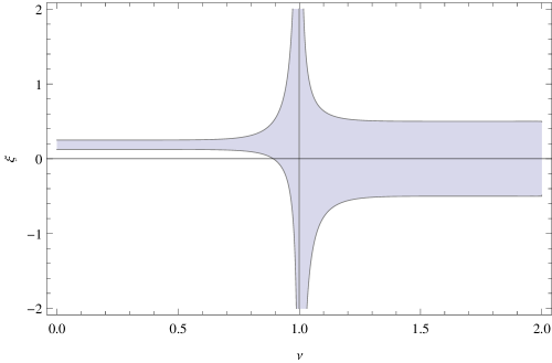
Figure 1: Permissible values of $\xi$ for a given $\nu$ — gray region. It should be noted that the conformal coupling, $\xi=1/6$, belongs to the whole permissible region; but that the minimal coupling, $\xi=0$, does not.

4.2 Permissible values of $\xi$ when $0<\nu<1$

When $0<\nu<1$, now eqs. (35) and (36) lead to

$$\frac{-\pi}{960c_{3}\nu\sin\nu\pi}+\frac{3c_{1}+2c_{3}}{16c_{3}}<\xi<\frac{\pi}{480c_{3}\nu\sin\nu\pi}+\frac{2c_{3}-3c_{1}}{8c_{3}},$$ (40)

which is illustrated in figure 1, on the left of the straight line $\nu=1$. Instead of eqs. (39), it follows from eq. (40),

$$-\frac{1}{38(1-\nu)}<\xi<\frac{1}{19(1-\nu)},\hskip 56.9055pt\nu\rightarrow 1.$$ (41)

Although there is no closed form available for $c_{3}$ when $\nu<1$, knowing that it behaves as $1/\nu^{2}$ when $\nu\rightarrow 0$, and using eq. (12), one readily obtains from eq. (40) that,

$$\frac{1}{8}<\xi<\frac{1}{4},\hskip 56.9055pt\nu\rightarrow 0.$$ (42)

Again, as $\nu$ decreases from $\nu=1$, the onset of the range in eq. (42) is rather quick (cf. figure 1).

5 Conclusion

This paper shows that the conical geometry around an infinite straight cosmic string restricts the values of the curvature coupling parameter $\xi$ when stable thermodynamic equilibrium of the scalar field with the background is required. The analysis is based on the low temperature behaviour of $\left<{\cal T}^{\alpha}{}_{\beta}\right>$ obtained from known formulas in the literature. The study adds new arguments to the conjecture that in any nontrivial background hot scalar radiation sets bounds on $\xi$ del15 .

The behaviour of the bounds on $\xi$, in the associated conical background [cf. eqs. (1) and (2)], is illustrated in figure 1 for $-\infty<{\cal D}<\pi$, i.e., $0<\nu<2$. The highlights are the asymptotic regimes in eqs. (38) and (39) (corresponding to attractive gravity), and those in eqs. (41) and (42) (corresponding to repulsive gravity). It can be seen that $\xi$ is restricted as long as the conical singularity is present, i.e., $\nu\neq 1$. Nevertheless, for cosmic strings of physical interest [cf. eq. (4)], only very large values of $|\xi|$ are unphysical.

Examining figure 1 one sees that $\nu$ is constrained even for the minimal coupling. That is, for $\xi=0$ stable thermodynamic equilibrium requires $\nu>\nu_{0}\approx 0.893$. This may appear unexpected since, when $\xi=0$, ${\cal T}^{\alpha}{}_{\beta}$ in the geometric background of a cosmic string reduces to the familiar canonical stress-energy-momentum tensor in Minkowski spacetime. In order to clarify this fact it should be recalled that the presence of the cosmic string “deforms” the vacuum, resulting in a vacuum expectation value of the observable ${\cal T}^{\alpha}{}_{\beta}$ which is different from that corresponding to the Minkowski vacuum (in a manner that resembles the well known Casimir effect). Indeed, when $\nu\neq 1$ (i.e., when the cosmic string is present), the vacuum expectation value in eq. (5) is nonzero when $\xi=0$. The cosmic string also affects thermal averages when $\xi=0$ [cf. eq. (21)] and eventually sets a constraint on $\nu$, as noted above. If one insists in having scalar radiation in stable thermodynamic equilibrium around a cosmic string for which $\nu<\nu_{0}$, then nonminimal coupling will be needed.

It should be noticed a rather curious feature regarding the range in eq. (42). Namely, it is precisely that corresponding to the allowed values of $\xi$ when the scalar field is near a reflecting Dirichlet wall in flat space del15 . [This fact looks less surprising if one recalls that $\nu\rightarrow 0$ corresponds to an infinite repulsive gravitational force (cf. section 2).]

It is inevitable to conjecture that the range in eq. (38) will still hold when $\nu>2$, though that needs confirmation by further calculations and analysis.

As seen in section 4, values of $\xi$ corresponding to negative $c_{V}$ must be excluded. Such values are unphysical since they would lead eventually to inhomogeneities, spoiling thermodynamic equilibrium. At this point one may recall that for a conformally coupled scalar field in the Hartle-Hawking thermal state around a Schwarzschild black hole, $c_{V}<0$ at the event horizon pag82 . It must be noted, however, that the cubic region of scalar radiation described in section 4 was examined by a stationary observer, to whom the ground state in the black hole background is the so called Boulware state (which, at infinity, becomes the Minkowski vacuum) can80 . It seems then that one should “renormalize” the energy density of the Hartle-Hawking state by subtracting that corresponding to the Boulware state dow78 . In so doing, a positive $c_{V}$ arises instead. A word of caution about this fact should be noted. Although the scalar radiation is in stable thermodynamic equilibrium with itself; it is not in stable thermodynamic equilibrium with the black hole, whose heat capacity is negative, as is fairly well known.

Although only a massless field was considered above, the results also apply to a massive scalar field with mass $M\ll T$ (and possibly to a massive scalar field of arbitrary mass, as happens in the case considered in ref. del15 ).

- (1) V. A. De Lorenci, L. G. Gomes and E. S. Moreira Jr., Hot scalar radiation setting bounds on the curvature coupling parameter, Class. Quant. Grav. 32 (2015) 085002 [arXiv:1304.6041].
- (2) A. G. Smith, Gravitational Effects of an Infinite Straight Cosmic String on Classical and Quantum Fields: Self-Forces and Vacuum Fluctuations, in the proceedings of The Formation and Evolution of Cosmic Strings Workshop, Cambridge U.K. (1989).
- (3) A. Vilenkin and E. P. S. Shellard, Cosmic Strings and Other Topological Defects, Cambridge University Press, Cambridge U.K. (1994).
- (4) D. Garfinkle, General relativistic strings, Phys. Rev. D 32 (1985) 1323.
- (5) T. W. B. Kibble, Cosmic Strings Reborn? [arXiv:astro-ph/0410073].
- (6) M. Sakellariadou, Cosmic Strings, Lect. Notes Phys. 718 (2007) 247 [arXiv:hep-th/0602276].
- (7) R. J. Slagter and S. Pan, A New Fate of a Warped 5D FLRW Model with a U(1) Scalar Gauge Field, Found. Phys. 46 (2016) 1075 [arXiv:1501.02843].
- (8) A. Staruszkiewicz, Gravitation theory in three-dimensional space, Acta. Phys. Pol. 24 (1963) 734.
- (9) G. ’t Hooft, Causality in (2+1)-dimensional gravity, Class. Quant. Grav. 9 (1992) 1335.
- (10) G. ’t Hooft, A Locally Finite Model for Gravity, Found. Phys. 38 (2008) 733 [arXiv:0804.0328].
- (11) S. Deser, R. Jackiw and G. ’t Hooft, Physical cosmic strings do not generate closed timelike curves, Phys. Rev. Lett. 68 (1992) 267.
- (12) V. P. Frolov, A. Pinzul and A. I. Zelnikov, Vacuum polarization at finite temperature on a cone, Phys. Rev. D 51 (1995) 2770.
- (13) M. E. X. Guimarães, Vacuum polarization at finite temperature around a magnetic flux cosmic string, Class. Quant. Grav. 12 (1995) 1705 [arXiv:gr-qc/9502003].
- (14) J. S. Dowker, Quantum field theory on a cone, J. Phys. A 10 (1977) 115.
- (15) J. S. Dowker, Thermal properties of Green’s functions in Rindler, de Sitter, and Schwarzschild spaces, Phys. Rev. D 18 (1978) 1856.
- (16) T. M. Helliwell and D. A. Konkowski, Vacuum fluctuations outside cosmic strings, Phys. Rev. D 34 (1986) 1918.
- (17) B. Linet, Quantum field theory in the space-time of a cosmic string, Phys. Rev. D 35 (1987) 536.
- (18) V. P. Frolov and E. M. Serebriany, Vacuum polarization in the gravitational field of a cosmic string, Phys. Rev. D 35 (1987) 3779.
- (19) J. S. Dowker, Vacuum averages for arbitrary spin around a cosmic string, Phys. Rev. D 36 (1987) 3742.
- (20) W. A. Hiscock, Semiclassical gravitational effects near cosmic strings, Phys. Lett. B 188 (1987) 317.
- (21) P. C. W. Davies and V. Sahni, Quantum gravitational effects near cosmic strings, Class. Quant. Grav. 5 (1988) 1.
- (22) B. Linet, The Euclidean thermal Green function in the spacetime of a cosmic string, Class. Quant. Grav. 9 (1992) 2429.
- (23) I. S. Gradshteyn and I. M. Ryzhik, Table of Integrals, Series, and Products, Academic Press, New York U.S.A. (2007).
- (24) D. N. Page, Thermal stress tensors in static Einstein spaces, Phys. Rev. D 25 (1982) 1499.
- (25) P. Candelas, Vacuum polarization in Schwarzschild spacetime, Phys. Rev. D 21 (1980) 2185.