Electrooptical Properties of Rydberg Excitons

Abstract

We show how to compute the electrooptical functions (absorption, reflection, and transmission) when Rydberg Exciton-Polaritons appear, including the effect of the coherence between the electron-hole pair and the electromagnetic field. With the use of Real Density Matrix Approach numerical calculations applied for Cu₂0 crystal are performed. We also examine in detail and explain the dependence of the resonance displacement on the state number and applied electric field strength. We report a good agreement with recently published experimental data.

I Introduction

The new avenue in modern semiconductor physics has been opened by outstanding experiment performed recently by Kazmierczuk et al Kazimierczuk who detected the large quasi particles known as Rydberg excitons in natural crystal of copper oxide. They have observed absorption lines associated with excitons of principal quantum numbers as large as $n=25$. One could expect that Rydberg excitons would have been described, in analogy to Rydberg atoms, by Rydberg series of hydrogen atom, but it has turned out that this generic method of description should have been revised. This is due to the fact that a size of a huge quasi particle, which in fact is a Rydberg exciton with high n, has a diameter more then two micrometers, which is much larger then the wavelength of light needed to create this exciton. Several theoretical approaches to calculate optical properties of Rydberg excitons have been presented Hofling ^-assmann_2016 . Schweiner et al Schweiner developed calculations of of the absorption spectrum on the ground of Toyozawa theory and calculated the main parameters for excitonic absorption line for yellow exciton series and emphasized that central-cell corrections have a major influence on the linewidth of the $2P$-exciton state. In our recent paper Zielinska.PRB we have proposed the method based on the Real Density Matrix Approach (RDMA) to obtain the analytical expressions for the optical functions of semiconductor crystals, including a high number of Rydberg excitons, taking into account the effect of anisotropic dispersion and the coherence of the electron and hole with the radiation field.

It is expected that the natural direction of development interest in Rydberg excitons is focused on Stark effect in such systems because this phenomenon may be used for the optical manipulations of excitons if there is an efficient coupling between the radiation field and excitonic systems far from the band edge. The copper oxide is a perfect candidate for such observations because due to high binding energy of orders of hundred meV and due to their large size, Rydberg excitons in Cu₂0 can exhibit very large electric dipole moments. These features provide that this system is appropriate to observe Stark effect experimentally. In semiconductors where the Wannier excitons have a small binding energy (as, for example, GaAs), the main effect of the applied electric field is the Stark shift of the excitonic resonances and changes in their oscillator strengths (see, for example, EPJ , RivistaGC for a review). In Cu₂O which is now the main semiconductor where Rydberg excitons are observed, even relatively high excitonic states have a binding energy which is larger than the corresponding ionization energy. Thus the excitonic character of the spectra is conserved, but new phenomena, as for example the appearance of symmetry forbidden states, with positions dependent on the applied field strength and on the state number, are observed Schoene ; Verhandl .

Actually, one of the aims of our theoretical paper is to extend the method presented in ref. Zielinska.PRB , which allowed to describe optical properties of Rydberg excitons, in order to obtain electrooptic functions (susceptibility, absorption reflection and transmission). Our approach has general character because it works for any exciton angular momentum number and for an arbitrary electric field. In particular, we derive an analytical expression for the electrosusceptibility, from which other electrooptical functions can be obtained. Since the electric field effects, increasing with the applied field strength and the state number, compete with the decreasing oscillator strength, we are able, having analytical expressions, to indicate the optimal excitation interval to observe the electrooptical effects. We also indicate the impact of the finite crystal size on the shape of the spectra, which was overlooked in the previous considerations. Therefore our predictions should be of interest for experimentalists.

The motivation of our considerations is also connected with with potential application of Rydberg excitons as solid-state switches. Due to their unusual features: long lifetimes, strong dipolar interactions and huge-size, they are expected to be implemented in quantum information technology. Kazimierczuk et al Kazimierczuk observed Rydberg blockade RB, which consists in reduction of excitonic absorption accompanied by increasing laser power for lines associated with large n, what means that only limited amount of Rydberg excitons is permitted in a well-localized space of the crystal. The idea of using dipolar Rydberg interaction to implement RB bases on the fact that in an ensemble of particles coupled by long-range dipolar interactions, only one particle can be excited at given time. The blockade originate from dipole-dipole interactions between Rydberg excitons unnecessary with the same n and is strongly influenced by their separation. This effect offers exciting possibilities for manipulating quantum bits stores in a single collective excitation in mezoscopic ensembles or for realizing scalable quantum logic gates and one implemented in solids would bring a lot of advantages for quantum information, for constructing all-optical switches and single-photon logic devices. Moreover, it is essential to have an additional mechanism for switching the dipole-dipole interaction, which in fact can be tuned on and off by Stark effect, therefore it is worth to go into details of the Stark effect in Rydberg excitons.

Our paper is organized as follows. In Sec. II we present the assumptions of considered model and solve the constitutive equation which give an analytical expression for the electrosusceptibility. We also use the obtained expression to compute the effective dielectric function, thanks to which the electrooptical functions (reflectivity, transmissivity, and absorption) are derived (section III). Next, in Sec. IV, the electrooptic functions are numerically analyzed for Cu₂O crystal for the purpose of realistic implementation of presented method. We examine in details changes of both real and imaginary part of electrosusceptibility, reflectivity and transmission under the influence of electric field. In Sec. V we draw conclusions of the model studied in this paper and we indicate the optimal range of energy for which Rydberg excitons could be experimentally observed.

II Density matrix formulation

Wannier-Mott excitons, treated as hydrogen-like particles, due to their small binding energy, are very receptive to the action of external fields (electric and/or magnetic). The external fields remove the degeneration of the excitonic energy levels and enhance the optical effects. Such effects were observed in the case of Rydberg excitons in Cu₂O Kazimierczuk ,Thewes . In what follows we describe the electrooptic properties of systems where the Rydberg excitons appear. As was recently shown in ref. Zielinska.PRB , the so-called real density matrix approach is very effective in describing the optical properties of Rydberg excitons. This approach was used in the past for the description of electrooptical effects (see, e.g., ref. EPJ and the references therein). We show below, that the specific properties of Rydberg excitons require a reformulation of the methods used in the past. As in ref. Zielinska.PRB , we do not enter into the quantum-mechanical explanation of the valence band structure of the Cu₂O. This explanation is given in details in the recent paper by Schweiner et al Schweiner_2016 . Here we treat the band structure and the related parameters as known, and use the scheme of ref. Zielinska.PRB for the situation, when the constant external electric field F is applied in the $z$ direction. The presented method starts with the constitutive equations, which have the form (for example, RivistaGC ,StB87 )

$$\dot{Y}(\textbf{R},\textbf{r}) = (-{\rm i}/\hbar)H_{eh}{Y}(\textbf{R},\textbf{r})+e\textbf{F}\textbf{r}-{\mit\Gamma}{Y}(\textbf{R},\textbf{r})$$ (1)

$$+ ({\rm i}/\hbar)\textbf{E}(\textbf{R})\textbf{M}(\textbf{r}),$$

where $Y$ is the bilocal coherent electron-hole amplitude (pair wave function), ${\bf R}$ jest is the excitonic center-of-mass coordinate, $\textbf{r}=\textbf{r}_{e}-\textbf{r}_{h}$ the relative coordinate, $\textbf{M}(\textbf{r})$ the smeared-out transition dipole density, ${\bf E}({\bf R})$ is the electric field vector of the wave propagating in the crystal. The coefficient $\mit\Gamma$ in the constitutive equation represents dissipative processes. We can expect a significant temperature-dependence of the spectra; microscopic analysis of damping parameters, which are the main temperature-dependent factors, requires future studies and will not be considered explicitly in this paper. The interaction with phonons and their role in determining the line shape, discussed recently by Schweiner at al (ref. Schweiner ) who have considered possible causes of line broadening, goes into the field of nonlinear optics and was in the past considered in the framework of the RDMA, for example by Schlösser (ref. Schlosser ) or in the case of EIT, in ref. EPJGC . In this paper we do not consider the interaction with phonons, and take the damping coefficients as phenomenological constants.

The smeared-out transition dipole density ${\bf M}({\bf r})$ is related to the bilocality of the amplitude $Y$ and describes the quantum coherence between the macroscopic electromagnetic field and the interband transitions. The two-band Hamiltonian $H_{eh}$ includes the electron- and hole kinetic energy terms, the electron-hole interaction potential and the confinement potentials. For details about the Hamiltonian see, for example, Zielinska.PRB . The coherent amplitude $Y$ defines the excitonic counterpart of the polarization

$$\textbf{P}(\textbf{R})=2\int{\rm d}^{3}r~{}\hbox{Re}~{}\left[\textbf{M}(\textbf{r})Y(\textbf{R},\textbf{r})\right],$$ (2)

which is than used in the Maxwell field equation

$$c^{2}\nabla_{R}^{2}\textbf{E}-\underline{\underline{\epsilon}}_{b}\ddot{\textbf{E}}(\textbf{R})=\frac{1}{\epsilon_{0}}\ddot{\textbf{P}}(\textbf{R}),$$ (3)

with the use of the bulk dielectric tensor $\underline{\underline{\epsilon}}_{b}$ and the vacuum dielectric constant $\epsilon_{0}$. In the present paper we solve the equations (1)-(3) with the aim to compute the electrooptical functions (reflectivity, transmission, and absorption) for the case of Cu₂O. In the following we will start with considering the bulk situation, where the center-of-mass motion is decoupled from the relative electron-hole motion and given by the term $\exp({\rm i}\textbf{k}\,{\textbf{R}})$ with the wave vector k resulting, in general, from the polariton dispersion relation Zielinska.PRB . We also assume the harmonic time dependence $\propto\exp(-{\rm i}\omega t)$. This assumptions allow to calculate the dielectric susceptibility. This will be achieved in by expanding the coherent amplitudes $Y$ in terms of eigenfunctions of the Hamiltonian $H_{eh}$. Let us note that the solution of the Schrödinger equation

$$H_{eh}\Psi+V(\textbf{r})\Psi=E\Psi,\quad V(\textbf{r})=e\textbf{Fr},$$ (4)

can be obtained only in an approximative way (perturbation calculus, variational method, matrix diagonalization etc.). Considering the cases of Cu₂O, when the applied field is of the order of 10 V/cm (Thewes ), we can compare the magnitude of the electron-hole pair attractive energy ($E_{n}=-R^{*}/n^{2}$ in the isotropic effective masses approximation) and the electric field energy $E_{field}=eFa^{*}_{n},a^{*}_{n}=n^{2}a^{*}$. For $n=16$ one has $E_{Coulomb}=0.39~{}\hbox{meV}$ and $E_{field}=0.38~{}\hbox{meV},\hbox{when}~{}F=15~{}\hbox{V/cm}$ (Thewes ). Thus the excitonic character of the spectra prevails and the applied electric field can be considered as perturbation. It is clear that, when external fields are applied, the full diagonalization of field- and band-mixing effects is more adequate to describe the optical properties, in particular when polarization dependence is considered. However, in the RDMA the band parameters, as e.g. the effective masses, are considered as field independent, and the fields are treated as perturbation operators. Such approach was merely applied in the past (for a recent review see EPJ ), for various nanostructures and field orientations, and was justified by the agreement with experimental data. The considered approximation is also justified by the fact, that the applied field strengths are much below the critical values for the fields (the ionization field for the electric field and the critical magnetic field). In the case of Cu₂0 the ionization field is of the order of 10⁶ V/cm, compared to the applied 15 or even 50 V/cm.

We assume the solution of the Eq. (4) in form of the solutions of an anisotropic Schrödinger equation $\varphi_{n\ell m}$ (see Appendix A for details)

$$\varphi_{n\ell m}(\textbf{r})=R_{n\ell m}(r)Y_{\ell m}(\theta,\phi),$$ (5)

where

$$R_{n\ell m}(r) = \left(\frac{2\eta_{\ell m}}{na^{*}}\right)^{3/2}\sqrt{\frac{(n-\ell-1)!}{2n(n+\ell)!}}\left(\frac{2\eta_{\ell m}r}{na^{*}}\right)^{\ell}$$ (6)

$$\times L_{n-\ell-1}^{2\ell+1}\left(\frac{2\eta_{\ell m}r}{na^{*}}\right)e^{-\eta_{\ell m}r/na^{*}},$$

with $\eta_{\ell m}$ defined by (30), and the Laguerre polynomials $L_{n}^{\alpha}(x)$ (for example, Grad )

$$L^{\alpha}_{n}(x) = \frac{1}{n!}e^{x}x^{-\alpha}\frac{{\rm d}^{n}}{{\rm d}x^{n}}\left(e^{-x}x^{n+\alpha}\right)$$ (7)

$$= \sum\limits_{m=0}^{n}(-1)^{m}{n+\alpha\choose n-m}\frac{x^{m}}{m!},$$

$Y_{\ell m}$ being the spherical harmonics. The energy eigenvalues relate to the eigenfunctions (5) have the form (see Eq. (37))

$$E_{n\ell m}=-\frac{\eta_{\ell m}^{2}}{n^{2}}R^{*},$$ (8)

where $n=1,2,\ldots,\ell=0,1,2,\ldots n-1,m=-\ell,-\ell+1,\ldots+\ell$. We see that the mass anisotropy removes the degeneracy with respect to the quantum number $\ell$, so that in this approach the higher order excitons $P$, $D$, $F$ etc. appear. When the electric field is directed along the z-axis, the perturbation operator $V$ has the form

$$V=eFz=eFr\cos\theta.$$ (9)

We look for the solutions of Eq. (1) in the form

$$Y=\sum\limits_{n\ell m}c_{n\ell m}R_{n\ell m}(r)Y_{\ell m}(\theta,\phi).$$ (10)

Inserting the above expansion into (1) we obtain the following system of equations for the expansion coefficients $c_{n_{1}\ell_{1}m_{1}}$ (for details, see Appendix B)

$$X_{n_{1}\ell_{1}m_{1}} = c_{n_{1}\ell_{1}m_{1}}W_{n_{1}\ell_{1}m_{1}}+\sum\limits_{n}c_{n\ell_{1}-1m_{1}}V^{(n)}_{\ell_{1}-1\ell_{1}m_{1}}$$ (11)

$$+ \sum\limits_{n}c_{n\ell_{1}+1m_{1}}V^{(n)}_{\ell_{1}\ell_{1}+1m_{1}}$$

where

$$V^{(nn_{1})}_{\ell_{1}-1\ell_{1}m_{1}}=eF\sqrt{\frac{\ell_{1}^{2}-m_{1}^{2}}{4\ell_{1}^{2}-1}}\int\,r^{2}{\rm d}r\,R_{n_{1}\ell_{1}m}rR_{n\ell_{1}-1m},$$

$$V^{(nn_{1})}_{\ell_{1}\ell_{1}+1m_{1}}=$$

$$=eF\sqrt{\frac{(\ell_{1}+1)^{2}-m_{1}^{2}}{(2\ell_{1}+1)(2\ell_{1}+3)}}\int\,r^{2}{\rm d}r\,R_{n_{1}\ell_{1}m}rR_{n\ell_{1}+1m},\quad$$

$$X_{n_{1}\ell_{1}m_{1}}=\mathcal{E}\int{\rm d}\Omega\int r^{2}{\rm d}rY_{\ell_{1}m_{1}}R_{n_{1}m\ell_{1}}M(r,\theta,\phi),$$

$$W_{n\ell m}=E_{g}+E_{n\ell m}+\frac{\hbar^{2}}{2M_{z}}k^{2}-\hbar\omega-{\rm i}{\mit\Gamma}=$$

$$=E_{Tn\ell m}-E+\frac{\hbar^{2}}{2M_{z}}k^{2}-{\rm i}{\mit\Gamma},$$ (12)

where $\mathcal{E}$ denotes the amplitude of the electric field. In all calculations we will use only the above matrix elements with $n=n_{1}$, denoting them by $V^{(n)}_{\ell_{1}-1\ell_{1}m_{1}},V^{(n)}_{\ell_{1}\ell_{1}+1m_{1}}.$ This is an approximation, which can be justified as follows. The spacing between the Rydberg states, at least for the states $n=2,..,7$ considered in this paper, is of the order of a few meV. Taking, for simplicity, Rydberg equal to 100 meV, one has the spacings (taking $\ell=0,m=0$ states) (meV) $E_{3}-E_{2}=14,E_{4}-E_{3}=4.75,E_{5}-E_{4}=2.25$, etc. On the other hand, the matrix elements V, collected in Table 1 and being the measure of the splitting between the Stark levels with the same principal number, are of the order between $10^{-3}$ and $10^{-1}$ meV, so that there are much smaller than the distances between the exciton states. Obviously, one should notice that the distances between the excitonic states decrease with the increasing number n, whereas the Stark splittings increase, and at a certain number the Stark splittings are greater than the spacing between the Rydberg states. The indication is that for higher numbers n one should take into account the interaction (in other words the matrix elements V) between different states, and not only within the same state. Besides, the method applied is not exactly the perturbation calculus, rather the matrix diagonalization, so its validity is not restricted by the value of the applied field.

We put the coherent amplitudes (10) into the equation (2), from which, when the center-of-mass motion is decoupled, one can obtain the susceptibility from the relation $\textbf{P}=\epsilon_{0}\chi(\omega,\textbf{k})\textbf{E}$. The dipole density vectors M should be chosen appropriate for P- or F- excitons, and we obtain (see also Zielinska.PRB )

$$\chi(\omega,\textbf{k}) = \Delta_{LT}^{(2)}\sum\limits_{n=2}^{N}C_{n10}f_{n1}+\Delta_{LT}^{(2)}\sum\limits_{n=4}^{N}f_{n3}C_{n30}$$ (13)

where for P excitons

$$C_{210} = \frac{W_{200}}{W_{200}W_{210}-\left(V_{010}^{(2)}\right)^{2}},$$

$$C_{310} = \frac{W_{300}W_{320}}{W_{300}\left[W_{310}W_{320}-\left(V_{120}^{(3)}\right)^{2}\right]-\left(V_{010}^{(3)}\right)^{2}W_{320}}.\qquad$$ (14)

For $n\geq 4$ we take the same expression as (II)

$$C_{n10} = \frac{W_{n00}}{W_{n00}W_{n10}-\left(V_{010}^{(n)}\right)^{2}}.$$

For F excitons when $\hbox{for}~{}n_{1}\geq 4$, taking into account $\ell=0,1,2,3$, one has (see also (70))

$$C_{n_{1}30} = \frac{W_{n_{1}20}W_{n_{1}10}W_{n_{1}00}}{\Delta}$$

$$- \frac{W_{n_{1}20}\left(V_{010}^{(n_{1})}\right)^{2}-W_{n_{1}00}\left(V_{120}^{(n_{1})}\right)^{2}}{\Delta},$$

$$\Delta = W_{n_{1}30}W_{n_{1}20}W_{n_{1}10}W_{n_{1}00}$$ (15)

$$-W_{n_{1}30}\left[W_{n_{1}20}\left(V_{010}^{(n_{1})}\right)^{2}-W_{n_{1}00}\left(V_{120}^{(n_{1})}\right)^{2}\right]$$

$$-\left(V^{(n_{1})}_{230}\right)^{2}\left[W_{n_{1}10}W_{n_{1}00}-\left(V_{010}^{(n_{1})}\right)^{2}\right].$$

For $F$ excitons, when $n\geq 5$, we can extend the basis taking $\ell=4,3,2,1,0$ and $m=0$, obtaining the expressions (B). In the above formulas $\Delta_{LT}^{(2)}$ denotes the longitudinal-transverse splitting energy. The explicit form of the oscillator strengths $f_{n1},f_{n3}$ for the isotropic case can be found in ref. Zielinska.PRB The oscillator strength $f_{n1}$ associated with P excitons is one order of magnitude greater than $f_{n3}$. Both values are roughly proportional to $n^{-3}$, especially for higher values of n (see Fig. 1).

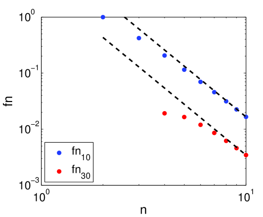
Figure 1: Oscillator strengths as a functon of exciton number $n$. Logarithmic scale is applied. Dashed line marks the linear regression for $n^{-3}$ relation.

The quantities of the type $W_{n00}$,$W_{n20}$ which enter into the above equations, correspond to S and D excitons. The matrix elements $V^{(n)}_{\ell\ell^{\prime}m}$ are calculated in Appendix C.

III Reflection and transmission spectra

In the previous considerations we treated the semiconductor crystal as unbounded. The real situation is different due to crystal finite size in all directions. Practically, the confined size in only one arbitrary chosen direction is considered and usually this direction is the same as electromagnetic wave vector. Concerning the experiments with Cu₂O one should notice that the dimension of the crystals examined experimentally exceeds the electromagnetic wave length, therefore the use of the long-wave-approximation is not well justified so we will compute the optical functions such as the transmissivity and reflectivity taking into account the finite crystal size and finite wavelength. We will obtain analytic expressions for the optical functions. These expressions will also include the impact of the applied constant electric field. In the description of the optical properties of excitons in finite semiconductors the excitonic Bohr radius plays an important role. Near the semiconductor surfaces there are layers where the excitons are created (or destroyed), the so-called exciton-free layers (”dead layers”). Mostly it is assumed that their thickness amounts to 2-3 excitonic Bohr radii. In the case of GaAs it gives about 30 nm. The excitons and related to them polaritons are formed in the remaining volume (”bulk”) of the crystal, and are responsible for the bulk susceptibility. The junction of layers with different dielectric properties is a complicated task and many works on this topic, including the so-called ABC problem, have been done over the past decades (for review see, for example, RivistaGC ; Bassani_2003 ; Agran2009 ). When we consider a particular case of GaAs thin layer of the thickness 150 nm, and the relevant excitonic Bohr radius is about 15 nm, then two excitonic Bohr radii correspond to 20 % of the crystal size. When we consider a Cu₂O slab, the situation is quite different. For a Cu₂O crystal of the size 30 $\mu$m Kazimierczuk , Thewes even the exciton state with n=25 has the extension of about 0.6 $\mu$m, so that the two Bohr radii correspond to 4 % of the crystal size. This means that, in the first approximation, we can neglect the dead layer effects. It does not mean that the dead layer and polariton effects are not important, as they can shift the resonance positions and affect the oscillator strengths (see also the discussion in ref. Schweiner ). The problem is that, when taking into account 25 excitonic states, we have at least 50 polaritonic waves (including the in- and outgoing polariton waves) so that the methods applied for the III-V and II-VI compounds (for example, ref. CBT96 ) cannot be applied for the case under consideration. This aspect requires future studies and will not be explicitly considered in this paper. Moreover it should be mentioned that different aspect of semiconductors’ geometry was considering by Schweiner et al Schweiner_2016 who have developed the method of investigation excitonic spectra taking into account the discrepancy of valence and conduction bands from parabolic shapes as well as their degeneracy and possible anisotropy.

The formation of excitons can be considered as a fast process leading to an effective dielectric function

$$\epsilon_{eff}=\epsilon_{b}+\chi=\epsilon_{b}+\chi_{1}+{\rm i}\,\chi_{2},$$ (16)

with the excitonic susceptibility defined in Eq. (13). Thus the electromagnetic wave in the crystal propagates in a medium characterized by the effective dielectric function. The crystal under consideration will be modeled by a slab with infinite extension in the $xy$-plane and the boundary planes $z=0,z=L$. With the sake of simplicity, the slab is located in vacuum. An monochromatic, linearly polarized electromagnetic wave propagates along $z$ axis. Its electric field is given by

$${\bf E}=(E_{x},0,0),\qquad E_{x}=E_{in}e^{{\rm i}k_{0}z-{\rm i}\omega t}\,,$$ (17)

where for vacuum

$$k_{0}=\frac{\omega}{c},$$ (18)

$\omega$ being the frequency, and $c$ the velocity of light. It is well known, the energy of the propagating wave will be divided into reflected and transmitted wave. The reflectivity, transmissivity, and absorption will be obtained from the relations

$$R=\left|\frac{E(0)}{E_{in}}-1\right|^{2}, T=\left|\frac{E(z=L)}{E_{in}}\right|^{2},$$ (19)

$$A = 1-R-T,$$

where $E(z)$ is the $x$-component of the wave electric field inside the crystal.

In the simplest approximation, neglecting the carrier confinement effects leading to the above mentioned ABC problem, we can use the effective dielectric function (16) and the resulting effective refractive index

$$n = \sqrt{\epsilon_{eff}}=n_{1}+{\rm i}\,n_{2},$$

$$n_{1} = \hbox{Re}\;n\approx\sqrt{\epsilon_{b}+\chi_{1}},$$ (20)

$$n_{2} = \hbox{Im}\;n\approx\frac{\chi_{2}}{2n_{1}}.$$

Then the reflectivity results from the standard formula

$$R=\left|\frac{1-n}{1+n}\right|^{2}=\frac{\left(1-n_{1}\right)^{2}+n_{2}^{2}}{\left(1+n_{1}\right)^{2}+n_{2}^{2}}.$$ (21)

Regarding the exceptional experiments by Kazimierczuk et al Kazimierczuk and Thewes et al. Thewes we can use the model of the multiple reflection and in the lowest order we get the following expression describing transmission

$$T=\frac{16|n|^{2}}{|(1+n)^{2}|^{2}}\;e^{-\alpha L}=$$

$$=\frac{16\left(n_{1}^{2}+n_{2}^{2}\right)}{\left[\left(1+n_{1}\right)^{2}-n_{2}^{2}\right]^{2}+4n_{2}^{2}\left(1+n_{1}\right)^{2}}\;e^{-\alpha L}.$$ (22)

Here

$$\alpha=2\frac{\hbar\omega}{\hbar c}\hbox{Im}\,n$$ (23)

denotes the absorption coefficient.

IV Results of specific calculations

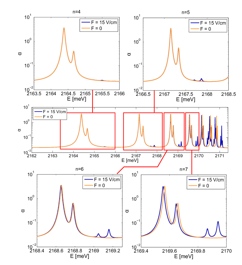
Figure 2: The bulk electroabsorption of a Cu₂O crystal calculated from the imaginary part of the susceptibility in the energetic region of $n=3-10$ excitonic states, for the electric field strengths $F=15~{}\hbox{V/cm}$ and $F=0$. The logarithmic scale is applied. Insets show the absorption spectrum near selected states.

We have performed numerical calculations of electrooptical functions (absorption, reflectivity, and transmissivity) for the Cu₂O crystal having in mind the experiments by Thewes et al Thewes , and Schöne et al Schoene . First, using the obtained expression for the susceptibility (13-II), we have calculated the electroabsorption, taking into account the lowest $n=2-10$ excitonic states. The parameters we used are the energies $E_{n\ell m}$, the gap energy $E_{g}$, the L-T energy $\Delta_{LT}^{(2)}$, and the dissipation parameter $\mit\Gamma$.

The energies $E_{n\ell m}$ were obtained from the relations (8) with the effective Rydberg energy $R^{*}$ and mass-anisotropy parameter $\gamma$. We have used the values $E_{g}=2172~{}\hbox{meV},R^{*}=86.981~{}\hbox{meV}$, $\Delta^{(2)}_{LT}=10~{}\mu\hbox{eV}$ which is common value in available literature, $\gamma=0.5351$, and phenomenological value of damping ${\mit\Gamma}=0.1~{}\hbox{meV}$. The results for the absorption, which seem the most important, are reported in Figs. 2-8.

In Fig. 2 we show the absorption spectrum in the region of $n=4-7$ excitons, for two values of the applied field. Since the absorption peaks decrease quite rapidly the logarithmic scale is applied. For clarity, we present in Fig. 3 the contributions of $P$ and $F$ excitons separately.

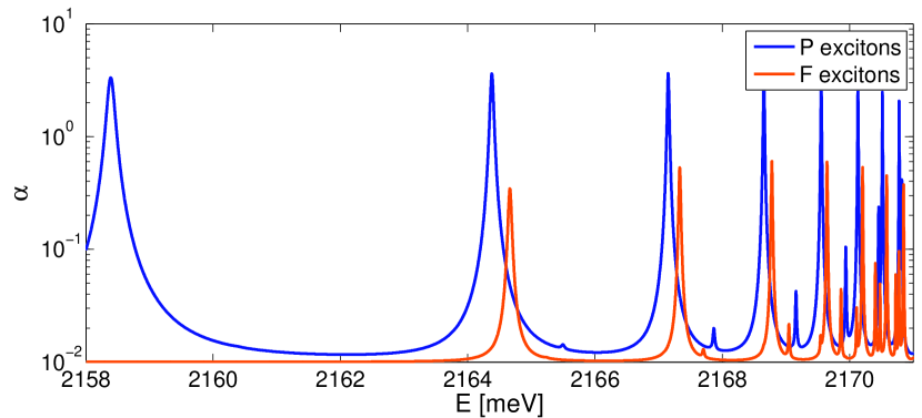
Figure 3: The bulk electroabsorption of a Cu₂O crystal, in the energetic region of $n=3-10$ excitonic states, for the electric field $F=15~{}\hbox{V/cm}$. The logarithmic scale is applied. The contributions of P and F excitons shown separately.

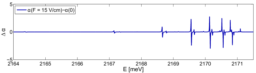
Figure 4: The difference $\Delta\alpha=\alpha(F)-\alpha(0)$, for $F=15~{}\hbox{V/cm}$ and in the range of $n=4-10$ excitonic states

The effects of the applied field are more evident when we display the difference $\Delta\alpha=\alpha(F)-\alpha(F=0)$. Such difference, for $F=15~{}\hbox{V/cm}$, is shown in Fig. 4. We observe that the numbers of additional peaks with increasing distances between them in comparison to the situation without an electric field. In our model this additional interaction is included in the matrix elements $V^{(n)}_{\ell_{1}-1\ell_{1}m_{1}}$ (Eq. (II)), which values increase with the state number (see Table 1). Therefore in the following we will focus our attention on higher number states. It should be stressed that for these states oscillator strengths are strong enough to warrant the robust and stable structure, which is important for possible further applications. In Fig. 5 we show the electroabsorption in the energetic region of $n=8-10$ excitonic states, for two values of the applied field strength. The $P$ and $F$ states are clearly distinguished.

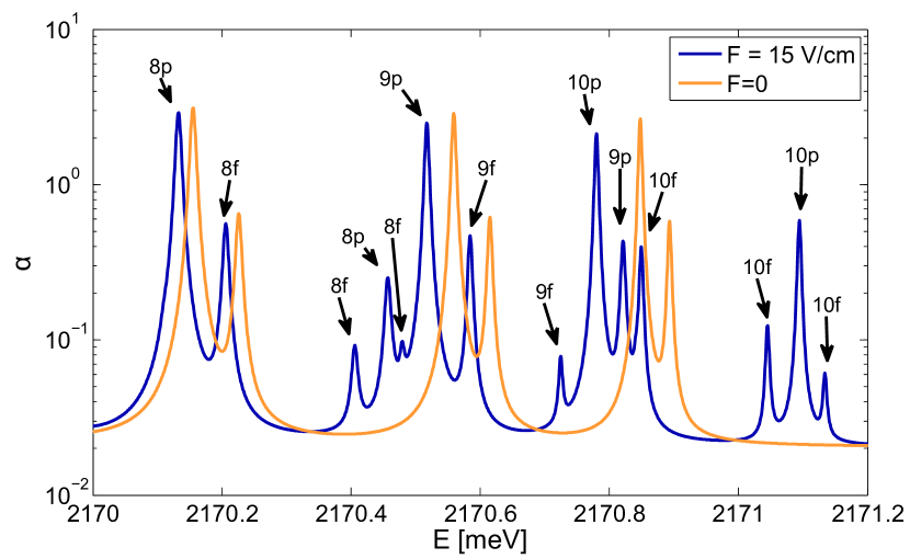
Figure 5: The bulk electroabsorption of $Cu_{2}O$ crystal calculated from imaginary part of susceptibility in the energetic region of $n=8-10$ excitonic states, for two electric field strengths $F=15~{}\hbox{V/cm}$ and $F=0$. The logarithmic scale is applied. There is some overlap in the identified states.

As it was reported in ref. Verhandl , the electric field strength can reach 50 V/cm so we performed numerical simulations to examine the influence of field strength on electrooptical properties of our system. It is visible in Fig. 6 where one can see the basic effect of the applied field: the Stark shift of the main peaks and the appearance of new resonances, especially evident in the case of F excitons.

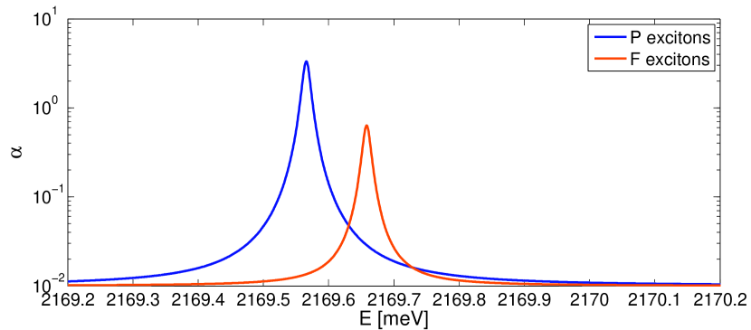
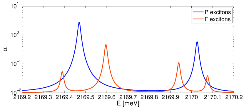
a) b)

Figure 6: a) The same as in Fig. 2, in the energetic region of $n=7$ exciton, without the electric field, b) for the field strength 50 V/cm

The changes in the absorption, as a function of the applied field strength, for the range (0,50) V/cm and near the $n=7$ state, are presented in Fig. 7 a. The absorption shape for three chosen values of the field are given in Fig. 7 b. The effect of the Stark shift and changes in the oscillator strength can be observed.

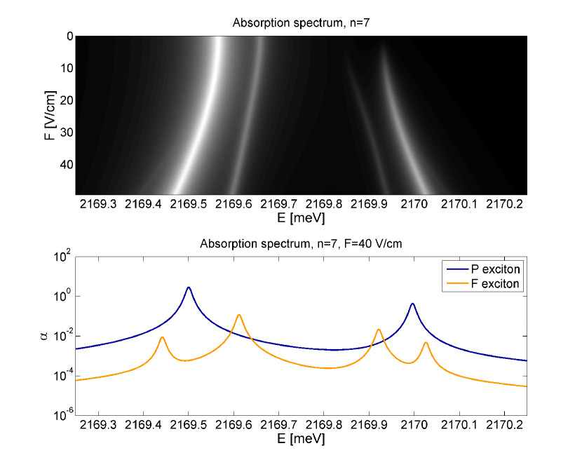
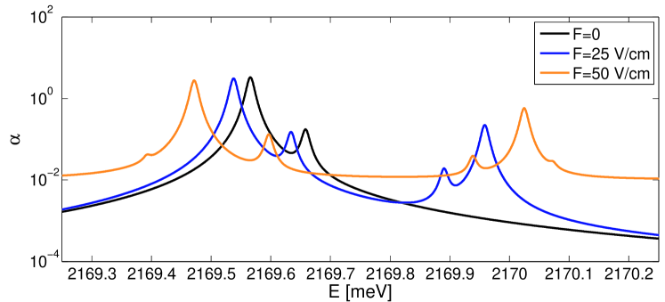
a) b)

Figure 7: a) The changes in the absorption, as a function of the applied field strength, for the range (0,50) V/cm, b) the same for three chosen values of the field strength

When we extend the energy interval to include more states, we observe evident mixing and overlapping of the lines of the neighboring states accompanied by spreading of Stark shifts with increasing of field strength. (Fig. 8). Our theoretical predictions are very close to the experimental results of Schöne et al Schoene .

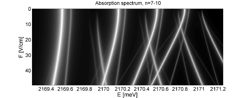
Figure 8: Absorption spectrum of Cu₂O crystal, in the energetic region of $n=7-10$ excitonic states as a function of the applied field strength

Our method allows to calculate both the real and the imaginary part of the susceptibility, without using the Kramers-Kronig relations. The results for the real part of $\chi$ are presented in Fig. 9. Having the real and imaginary part of the susceptibility, we have been able to get the effective dielectric function from (16) and other optical functions, in particular, the reflection coefficient (Eq. (21)), which is shown in Fig. 10 a). Its shape resembles the real part of the susceptibility. We notice the red shift of the main peaks, changes in the oscillator strength, appearance of new peaks when the field is applied, and decreasing the effects for the energies above the 2.171 eV. Similar as it was done for the electroabsorption (Fig. 4), we plot the difference $\Delta R=R(F)-R(0)$ for the energetic region of $n=8-10$ excitonic resonances (Fig. 10 b). It can be seen that the electrooptical effects are noticeable, maxima of reflectivity are back-shifted and due to electric field new peaks have occurred.

Finally, making use of Eq. (III), we have calculated the transmissivity of the considered above Cu₂O crystal, taking the size $L=30~{}\mu\hbox{m}$. The results for the transmissivity $T$ and the difference $\Delta T=T(F)-T(0)$ are shown in Fig. 10 c,d. The same tendency as for reflectivity can be observed.

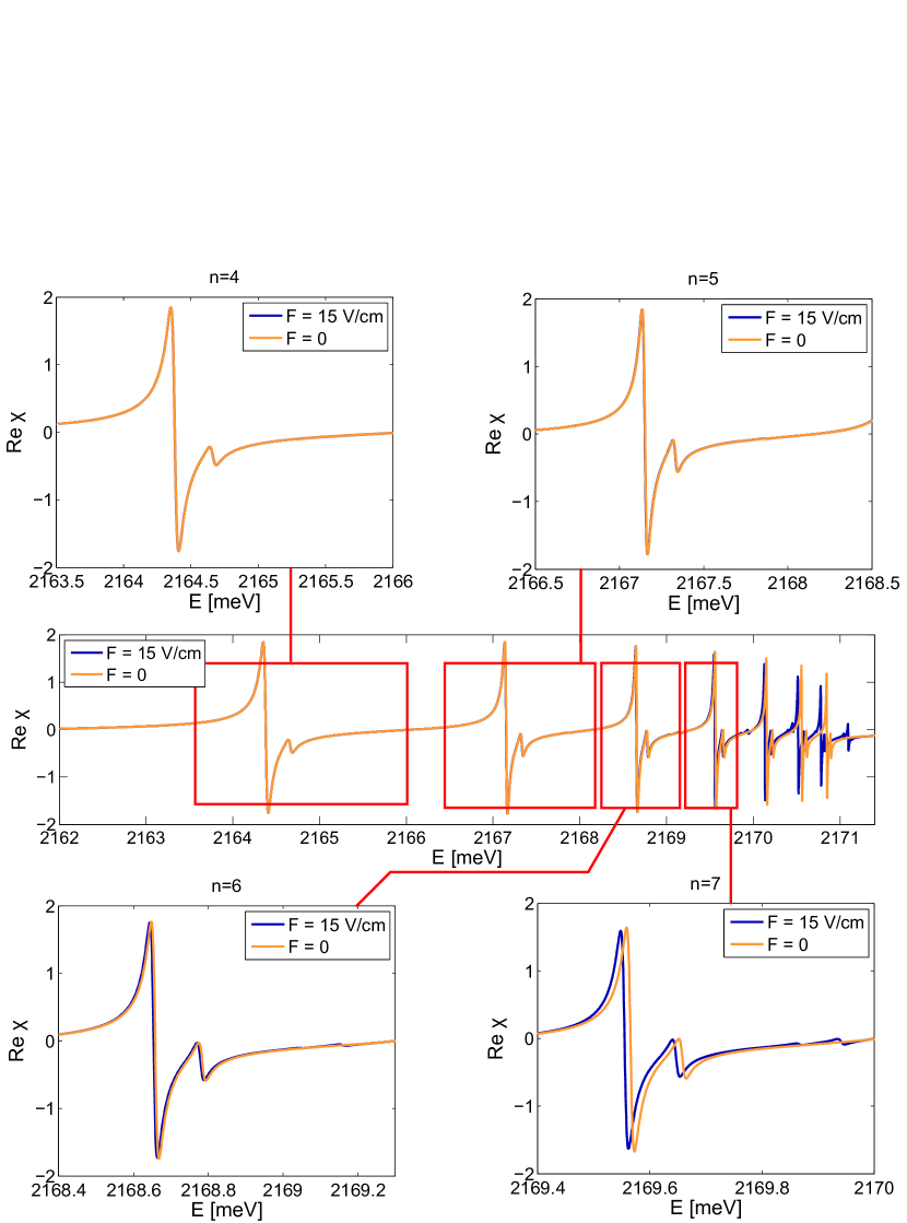
Figure 9: The real part of susceptibility of Cu₂O crystal in the energetic region of $n=4-10$ excitonic states, for the electric field $F=15~{}\hbox{V/cm}$ and $F=0$. The logarithmic scale is applied. Insets show absorption spectrum near selected states.

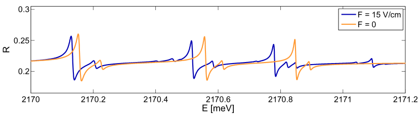
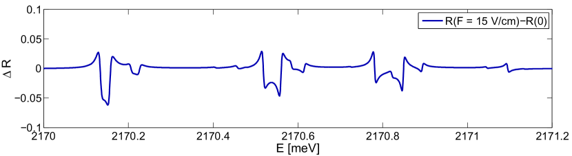
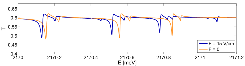
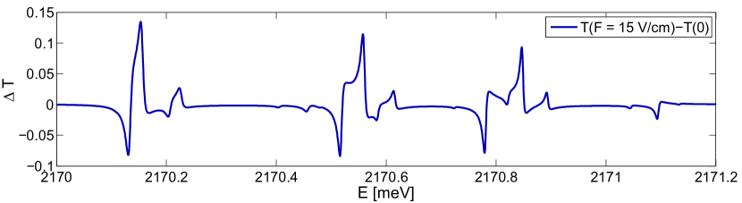
a) b) c) d)

Figure 10: a) The reflection coefficient of a Cu₂O crystal, in the energetic region of $n=8-10$ excitonic states, for two values of the electric field. b) The difference $\Delta R=R(F)-R(F=0)$ for $F=15~{}\hbox{V/cm}$. c) The transmissivity $T$, and d) $\Delta T=T(F)-T(0)$, for $F=15~{}\hbox{V/cm}$.

V Conlusions

The main results of our paper can be summarized as follows. We have proposed a procedure based on the RDMA approach that allows to obtain analytical expressions for the electrooptical functions of semiconductor crystals including high number Rydberg excitons. Our results have general character because arbitrary exciton angular momentum number and arbitrary applied field strength are included. We have chosen the example of cuprous dioxide, inspired by the recent experiment by Kazimierczuk et al Kazimierczuk . We have calculated the electrooptical functions (susceptibility, absorption, reflection, and transmission), obtaining a good agreement between the calculated and the experimentally observed spectra. Our results confirm the fundamental peculiarity of Stark effect - shifting, splitting and, as a result for higher excitonic states, mixing of spectral lines. In particular, we obtained the splitting of P and F excitons, with increasing number of peaks corresponding to increasing state number. We could assess the observed peaks to excitonic states, which are symmetry forbidden when the electric field is absent. On the basis of our theory we have predicted the range of energy where one could observe the Stark splitting and shifting for Rydberg excitons. All these interesting features of excitons with high $n$ number which are examined and discussed on the basis on our theory might possibly provide deep insight into the nature of Rydberg excitons in solids and provoke their application to design all-optical flexible switchers and future implementation in quantum information processing. Rydberg excitons in cuprous oxide are also promising candidates for observing the influence of magnetic fields effects. Very recently the transmission spectrum of Cu₂O yellow series was registered in magnetic fields for states with high n number showing extraordinary complex splitting pattern of levels.assmann_2016 The approach similar to described above could be used to analyze this experiment.

Appendix A Anisotropic Schrödinger equation

Below we follow the calculations from ref. Zeitschrift , correcting and supplementing them. Consider a two band semiconductor with an isotropic conduction band (electron) mass $m_{e}$ and anisotropic hole mass with the components $m_{h\parallel},m_{z}$, with corresponding reduced masses

$$\frac{1}{\mu_{\parallel}}=\frac{1}{m_{e}}+\frac{1}{m_{h\parallel}},\qquad\frac{1}{\mu_{z}}=\frac{1}{m_{e}}+\frac{1}{m_{hz}}.$$ (24)

Anisotropic Schrödinger equation for the relative electron-hole motion, with the above reduced masses and with a screened Coulomb interaction, has the form

$$\biggl{[}-\frac{\hbar^{2}}{2\mu_{\parallel}}\left(\frac{\partial^{2}}{\partial x^{2}}+\frac{\partial^{2}}{\partial y^{2}}\right)-\frac{\hbar^{2}}{2\mu_{z}}\frac{\partial^{2}}{\partial z^{2}}$$

$$-\frac{e^{2}}{4\pi\epsilon_{0}\epsilon_{b}\sqrt{x^{2}+y^{2}+z^{2}}}\biggr{]}\psi=E\psi.$$ (25)

Using scaled variables

$$x=\xi a^{*},\qquad y=\eta a^{*},\qquad z=\zeta\gamma a^{*},\quad\gamma=\sqrt{\mu_{\parallel}/\mu_{z}},$$

$$a^{*-1}=\frac{\mu_{\parallel}}{\hbar^{2}}\frac{e^{2}}{4\pi\epsilon_{0}\epsilon_{b}},\qquad\frac{2\mu_{\parallel}}{\hbar^{2}}a^{*2}=\frac{1}{R^{*}},$$ (26)

we transform Eq. (A) into

$$\left(\nabla_{\rho^{2}}-\frac{2}{\rho\sqrt{\sin^{2}\theta+\gamma^{2}\cos^{2}\theta}}\right)\psi(\rho,\theta,\phi)=\varepsilon\psi(\rho,\theta,\phi)$$ (27)

where $\rho=\sqrt{\xi^{2}+\eta^{2}+\zeta^{2}},\qquad\varepsilon=E/R^{*},$ $\nabla_{\rho^{2}}$ is the common Laplace operator in spherical coordinates. We are looking for the solution in the form

$$\psi(\rho,\theta,\phi)=\sum\limits_{\ell}R_{\ell}(\rho)Y_{\ell m}(\theta,\phi).$$ (28)

Multiplicating both sides with $Y^{*}_{\ell^{\prime}m^{\prime}}$, integrating and taking into account only the diagonal terms $\ell=\ell^{\prime},m=m^{\prime}$ we obtain the following equation for the radial part $R$

$$\left[\frac{{\rm d}^{2}}{{\rm d}\rho^{2}}+\frac{2}{\rho}\frac{\rm d}{{\rm d}\rho}-\kappa^{2}+\frac{2}{\rho}\eta_{\ell m}-\frac{\ell(\ell+1)}{\rho^{2}}\right]R=0,$$ (29)

with

$$\eta_{\ell m}=\int\limits_{0}^{2\pi}{\rm d}\phi\int\limits_{0}^{\pi}\sin\theta\,{\rm d}\theta\frac{\left|Y_{\ell m}\right|^{2}}{\sqrt{\sin^{2}\theta+\gamma^{2}\cos^{2}\theta}},$$ (30)

and with $\kappa^{2}=-\varepsilon$, assuming that we consider only the bound states. Some values for $\eta_{\ell m}$ were given in Refs. Zielinska.PRB and Zeitschrift . Mostly $\gamma$ is close to 1. In this case, to a good approximation

$$\eta_{\ell m}=1+\frac{(1-\gamma)(2\ell^{2}+2\ell-1-2m^{2})}{2(2\ell-1)(2\ell+3)}.$$ (31)

Making use of substitutions

$$z=2\kappa\rho,\quad\lambda=\frac{\eta_{\ell m}}{\kappa},\quad F=R(z)z,\quad\mu=\ell+\frac{1}{2},$$ (32)

we transform (29) into the equation

$$\frac{{\rm d}^{2}}{{\rm d}z^{2}}F+\left(-\frac{1}{4}+\frac{\lambda}{z}+\frac{(1/4)-\mu^{2}}{z^{2}}\right)F=0.$$ (33)

The above equation has two linearly independent solutions $M_{\lambda,\mu},W_{\lambda,\mu}$ known as the Whittaker functions. They are related to the more familiar Kummer functions (confluent hypergeometric functions) by the relations

$$M_{\lambda,\mu}(z)=z^{\mu+1/2}e^{-z/2}M\left(\mu-\lambda+\frac{1}{2},2\mu+1,z\right),$$

$$W_{\lambda,\mu}(z)=z^{\mu+1/2}e^{-z/2}U\left(\mu-\lambda+\frac{1}{2},2\mu+1,z\right).$$

We choose the function $M$ which is finite for $z=0$ and, with respect to the relations (32) we obtain the radial part $R$ in the form

$$R=N(2\kappa\rho)^{\ell}e^{-\kappa\rho}M\left(\ell+1-\lambda,2\ell+2,2\kappa\rho\right),$$ (34)

$N$ being the normalization constant. The function $R$ is finite for $\rho\to\infty$ when the first argument of the Kummer function is 0 or negative integer. Thus

$$\ell+1-\frac{\eta_{\ell m}}{\kappa}=-N,$$ (35)

which gives

$$\frac{\eta_{\ell m}}{\kappa}=N+\ell+1=n,$$ (36)

and, finally

$$\varepsilon=-\frac{\eta_{\ell m}^{2}}{n^{2}}.$$ (37)

Inserting the result for $\kappa$ into (34) we obtain the radial function $R$ in the form

$$R(\rho)=R_{n\ell m}(\rho)=N_{n\ell m}\left(\frac{2\eta_{\ell m}\rho}{n}\right)^{\ell}e^{-\eta_{\ell m}\rho/n}$$

$$\times\,M\left(-n+\ell+1,2\ell+2,\frac{2\eta_{\ell m}\rho}{n}\right).$$ (38)

Using the integral (for example, Landau )

$$J_{\nu}=\int\limits_{0}^{\infty}e^{-kz}z^{\nu-1}\left[M(-n,\gamma,kz)\right]^{2}{\rm d}z$$

$$=\frac{\Gamma(\nu)\;n!}{k^{\nu}\gamma(\gamma+1)\ldots(\gamma+n-1)}\biggl{\{}1+\frac{n(\gamma-\nu-1)(\gamma-\nu)}{1^{2}\cdot\gamma}$$

$$+\frac{n(n-1)(\gamma-\nu-2)(\gamma-\nu-1)(\gamma-\nu)(\gamma-\nu+1)}{1^{2}\cdot 2^{2}\cdot\gamma(\gamma+1)}+\ldots\biggr{\}}$$

we obtain the normalization constant in the form

$$N_{n\ell m}=\left(\frac{2\eta_{\ell m}}{n}\right)^{3/2}\frac{1}{(2\ell+1)!}\sqrt{\frac{(n+\ell)!}{2n(n-\ell-1)!}}.$$ (39)

Thus the radial part of the solution of the anisotropic Schrödinger equation has the form

$$R_{n\ell m}(\rho)=\left(\frac{2\eta_{\ell m}}{n}\right)^{3/2}\frac{1}{(2\ell+1)!}\sqrt{\frac{(n+\ell)!}{2n(n-\ell-1)!}}$$

(40)

$$\times\left(\frac{2\eta_{\ell m}\rho}{n}\right)^{\ell}e^{-\eta_{\ell m}\rho/n}M\left(-n+\ell+1,2\ell+2,\frac{2\eta_{\ell m}\rho}{n}\right).$$

Using the relation

$$L_{N}^{\alpha}(x)={N+\alpha\choose N}M(-N,\alpha+1,x)$$

between the Kummer function and the Laguerre polynomials, we can express the radial function $R$ in terms of them

$$R_{n\ell m}(\rho)=\left(\frac{2\eta_{\ell m}}{n}\right)^{3/2}\sqrt{\frac{(n-\ell-1)!}{2n(n+\ell)!}}\left(\frac{2\eta_{\ell m}\rho}{n}\right)^{\ell}$$

$$\times L_{n-\ell-1}^{2\ell+1}\left(\frac{2\eta_{\ell m}\rho}{n}\right)e^{-\eta_{\ell m}\rho/n}.$$ (41)

Appendix B Derivation of the expansion coefficients

Inserting the expansion (10) into (1) and making use of the relations

$$\cos\theta\,Y_{\ell m} = \sqrt{\frac{(\ell+1+m)(\ell+1-m)}{(2\ell+1)(2\ell+3)}}Y_{\ell+1m}$$

$$+ \sqrt{\frac{(\ell+m)(\ell-m)}{(2\ell+1)(2\ell-1)}}Y_{\ell-1m},$$

$$\langle\ell_{1}m_{1}|\cos\theta|\ell_{2}m_{2}\rangle \neq 0\quad\hbox{ if}\quad m_{1}=m_{2}~{}\hbox{and}~{}\ell_{1}=\ell_{2}\pm 1\quad$$

$$\langle\ell m|\cos\theta|\ell-1m\rangle = \sqrt{\frac{\ell^{2}-m^{2}}{4\ell^{2}-1}},$$ (42)

and making use of the orthogonality properties of the eigenfunctions $R_{n\ell},Y_{\ell m}$ we obtain the system of equations (11) for the expansion coefficients. The equations (11) form, in general, an infinite system of linear equations. Therefore a certain cut-off must be applied. Having in mind the properties of Cu₂O we put $n=n_{1}$, i.e. we neglect the interaction between the states with different quantum number $n$. It is due to the fact that the energy differences between the states are much larger than the perturbations caused by the electric field. In consequence, the infinite system of equations is reduced to a set of subsystems of equations for each value of $n$. The subsystems consist, in general, of $2n^{2}$ equations labeled by different values of $\ell$ and $m$. With respect to the properties of Cu₂O, we will consider the $P$ excitons ($\ell=1$) and $F$ excitons ($\ell=3$). The lowest $P$ exciton state is given by $n=2,\ell=1,m=0$. From (11), with M given by Zielinska.PRB

$${\bf M}({\bf r}) = \textbf{e}_{r}\,M_{10}\frac{r+r_{0}}{2r^{2}r_{0}^{2}}e^{-r/r_{0}}=\textbf{e}_{r}M(r)=$$ (43)

$$= \textbf{i}M_{10}\frac{r+r_{0}}{4{\rm i}r^{2}r_{0}^{2}}\sqrt{\frac{8\pi}{3}}\left(Y_{1,-1}-Y_{1,1}\right)e^{-r/r_{0}}+$$

$$+ \textbf{j}M_{10}\frac{r+r_{0}}{4r^{2}r_{0}^{2}}\sqrt{\frac{8\pi}{3}}\left(Y_{1,-1}+Y_{1,1}\right)e^{-r/r_{0}}+$$

$$+ \textbf{k}M_{10}\frac{r+r_{0}}{2r^{2}r_{0}^{2}}\sqrt{\frac{4\pi}{3}}Y_{10}e^{-r/r_{0}},$$

and its $Y_{10}$ component, one obtains 4 equations

$$\begin{array}[]{rcccccc}W_{200}c_{200}&+&V^{(2)}_{010}c_{210}&&&=&0\\ V^{(2)}_{010}c_{200}&+&W_{210}c_{210}&&&=&X_{210}\\ &&&W_{211}c_{211}&&=&0\\ &&&&W_{21-1}c_{21-1}&=&0\end{array}$$ (47)

where we took only the allowed combinations for the $n,\ell,m$. Thus we obtain

$$c_{210}=C_{210}X_{210}=\frac{W_{200}X_{210}}{W_{200}W_{210}-\left(V^{(2)}_{010}\right)^{2}}.$$ (49)

For the $P,n=3$ exciton state we use $n^{2}=9$ combinations:

$$\begin{array}[]{rcccccc}300(x_{1})&310(x_{2})&311(x_{3})&31-1(x_{4})&&&\\ 320(x_{5})&321(x_{6})&32-1(x_{7})&&&&\\ 322(x_{8})&32-2(x_{9})&&&&&\\ \end{array}$$ (53)

and obtain equations

$$\begin{array}[]{rccccccccc}W_{300}x_{1}&+&V_{010}^{(3)}x_{2}&+\ldots&&&&&=&0\\ V_{010}^{(3)}x_{1}&+&W_{310}x_{2}&+\ldots&&+V_{120}^{(3)}x_{5}&&&=&X_{310}\\ &&&W_{311}x_{3}&&\ldots&+V_{121}^{(3)}x_{6}&&=&0\\ &&&&W_{31-1}x_{4}&&\ldots&+V_{12-1}^{(3)}x_{7}&=&0\\ &&V_{120}^{(3)}x_{2}&&\ldots&+W_{320}x_{5}&&&=&0\\ &&&V_{121}^{(3)}x_{3}&&\ldots&+W_{321}x_{6}&&=&0\\ &&&&V_{12-1}^{(3)}x_{4}&&\ldots&+W_{32-1}x_{7}&=&0\\ \end{array}$$ (61)

where $c_{300}=x_{1},c_{310}=x_{2}$ etc., with regard to (53). For remaining the remaining coefficients we have $x_{8}=x_{9}=0$. The resulting coefficient $c_{310}=C_{310}X_{310}$ is given by the formula (14). In the expressions for $C_{210}$ and $C_{n10}$ one can separate the real and imaginary part, obtaining

$$C_{n10} = \frac{(E_{Tn00}-E)\left[\left(E_{Tn00}-E\right)\left(E_{Tn10}-E\right)-\left(V_{010}^{(n)}\right)^{2}-{\mit\Gamma}^{2}\right]+\left(E_{Tn10}+E_{Tn00}-2E\right){\mit\Gamma}^{2}}{\left[\left(E_{Tn00}-E\right)\left(E_{Tn10}-E\right)-\left(V_{010}^{(n)}\right)^{2}-{\mit\Gamma}^{2}\right]^{2}+\left(E_{Tn10}+E_{Tn00}-2E\right)^{2}{\mit\Gamma}^{2}}$$ (62)

$$+\;{\rm i}{\mit\Gamma} \frac{\left(E_{Tn00}-E\right)^{2}+\left(V_{010}^{(n)}\right)^{2}+{\mit\Gamma}^{2}}{\left[\left(E_{Tn00}-E\right)\left(E_{Tn10}-E\right)-\left(V_{010}^{(n)}\right)^{2}-{\mit\Gamma}^{2}\right]^{2}+\left(E_{Tn10}+E_{Tn00}-2E\right)^{2}{\mit\Gamma}^{2}}\;.$$

Clearly $\hbox{Im}\;C_{n10}>0$. Introducing notation

$$E_{\ell}^{(n)} = E_{Tn\ell 0}-E,$$

$$W_{n\ell 0}(k=0) = E_{\ell}^{(n)}-{\rm i}{\mit\Gamma},$$ (63)

$$R_{\ell\ell_{1}}^{(n)} = E_{\ell}^{(n)}E_{\ell_{1}}^{(n)}-{\mit\Gamma}^{2},$$

$$S_{\ell\ell_{1}}^{(n)} = E_{\ell}^{(n)}+E_{\ell_{1}}^{(n)},$$

we put eq. (62) into a more compact form

$$C_{n10} = \frac{E_{0}^{(n)}\left[R_{01}^{(n)}-\left(V_{010}^{(n)}\right)^{2}\right]+S_{01}^{(n)}{\mit\Gamma}^{2}}{\left[R_{01}^{(n)}-\left(V_{010}^{(n)}\right)^{2}\right]^{2}+\left(S_{01}^{(n)}\right)^{2}{\mit\Gamma}^{2}}+\;{\rm i}{\mit\Gamma}\frac{\left(E_{0}^{(n)}\right)^{2}+\left(V_{010}^{(n)}\right)^{2}+{\mit\Gamma}^{2}}{\left[R_{01}^{(n)}-\left(V_{010}^{(n)}\right)^{2}\right]^{2}+\left(S_{01}^{(n)}\right)^{2}{\mit\Gamma}^{2}}\;.$$ (64)

For $F$ excitons, when $n_{1}\geq 4,\ell=3,2,1,0,m=0$, we obtain the following equations for the expansion coefficients

$$\begin{array}[]{cccccc}c_{n_{1}30}W_{n_{1}30}&+c_{n_{1}20}V^{(n_{1})}_{230}&&&=X_{n_{1}30},\\ c_{n_{1}30}V^{(n_{1})}_{230}&+c_{n_{1}20}W_{n_{1}20}&+c_{n_{1}10}V_{120}^{(n_{1})}&&=0,\\ &c_{n_{1}20}V^{(n_{1})}_{120}&+c_{n_{1}10}W_{n_{1}10}&+c_{n_{1}00}V_{010}^{(n_{1})}&=0,\\ &&c_{n_{1}10}V_{010}^{(n_{1})}&+c_{n_{1}00}W_{n_{1}00}&=0.\end{array}$$ (69)

with the result for the relevant coefficient

$$c_{n_{1}30}=X_{n_{1}30}C_{n_{1}30}=X_{n_{1}30}\frac{W_{n_{1}20}W_{n_{1}10}W_{n_{1}00}-W_{n_{1}20}\left(V_{010}^{(n_{1})}\right)^{2}-W_{n_{1}00}\left(V_{120}^{(n_{1})}\right)^{2}}{\Delta},$$ (70)

where

$$\Delta=\left|\begin{array}[]{cccccc}W_{n_{1}30}&V^{(n_{1})}_{230}&0&0&\\ V^{(n_{1})}_{230}&W_{n_{1}20}&V_{120}^{(n_{1})}&0&\\ 0&V^{(n_{1})}_{120}&W_{n_{1}10}&V_{010}^{(n_{1})}&\\ 0&0&V_{010}^{(n_{1})}&W_{n_{1}00}&\\ \end{array}\right|$$

$$=W_{n_{1}30}\left[W_{n_{1}20}W_{n_{1}10}W_{n_{1}00}-W_{n_{1}20}\left(V_{010}^{(n_{1})}\right)^{2}-W_{n_{1}00}\left(V_{120}^{(n_{1})}\right)^{2}\right]$$

$$-\left(V^{(n_{1})}_{230}\right)^{2}\left[W_{n_{1}10}W_{n_{1}00}-\left(V_{010}^{(n_{1})}\right)^{2}\right].$$

Using the definitions (B), $C_{n_{1}30}$ can be put into the form

$$C_{n_{1}30} = \frac{ac-bd}{a^{2}+b^{2}}+{\rm i}\;\frac{ad+bc}{a^{2}+b^{2}},$$

$$a = R^{(n_{1})}_{01}R^{(n_{1})}_{23}+\left(V_{010}^{(n_{1})}\right)^{2}\left(V^{(n_{1})}_{230}\right)^{2}-{\mit\Gamma}^{2}S_{01}^{(n_{1})}S_{23}^{(n_{1})}-R^{(n_{1})}_{01}\left(V^{(n_{1})}_{230}\right)^{2}$$ (72)

$$-R^{(n_{1})}_{03}\left(V^{(n_{1})}_{120}\right)^{2}-R^{(n_{1})}_{23}\left(V^{(n_{1})}_{010}\right)^{2},$$

$$b = {\mit\Gamma}\left[R^{(n_{1})}_{01}S_{23}^{(n_{1})}+R^{(n_{1})}_{23}S_{01}^{(n_{1})}-S_{01}^{(n_{1})}\left(V^{(n_{1})}_{230}\right)^{2}-S_{03}^{(n_{1})}\left(V_{120}^{(n_{1})}\right)^{2}-S_{23}^{(n_{1})}\left(V_{010}^{(n_{1})}\right)^{2}\right]$$

$$c = E^{(n_{1})}_{2}R^{(n_{1})}_{01}-{\mit\Gamma}^{2}S_{01}^{(n_{1})}-E^{(n_{1})}_{2}\left(V_{010}^{(n_{1})}\right)^{2}-E^{(n_{1})}_{0}\left(V_{120}^{(n_{1})}\right)^{2},$$

$$d = {\mit\Gamma}\left[\left(V_{010}^{(n_{1})}\right)^{2}+\left(V_{120}^{(n_{1})}\right)^{2}-S_{01}^{(n_{1})}E^{(n_{1})}_{2}-R^{(n_{1})}_{01}\right].$$

For $F$ excitons, when $n\geq 5$, we can extend the basis taking $\ell=4,3,2,1,0$ and $m=0$, obtaining

$$c_{n_{1}30} = X_{n_{1}30}\frac{W_{n_{1}40}\left[W_{n_{1}20}W_{n_{1}10}W_{n_{1}00}-W_{n_{1}20}\left(V_{010}^{(n_{1})}\right)^{2}-W_{n_{1}00}\left(V_{120}^{(n_{1})}\right)^{2}\right]}{\Delta},$$

$$\Delta = \left[W_{n_{1}40}W_{n_{1}30}-\left(V_{340}^{(n_{1})}\right)^{2}\right]\left[W_{n_{1}20}W_{n_{1}10}W_{n_{1}00}-W_{n_{1}20}\left(V_{010}^{(n_{1})}\right)^{2}-W_{n_{1}00}\left(V_{120}^{(n_{1})}\right)^{2}\right]$$ (73)

$$-W_{n_{1}40}\left(V^{(n_{1})}_{230}\right)^{2}\left[W_{n_{1}10}W_{n_{1}00}-\left(V_{010}^{(n_{1})}\right)^{2}\right].$$

Appendix C Derivation of the matrix elements $V^{(n)}_{\ell_{1}-1\ell_{1}m_{1}}$

The matrix elements follow from the definitions (II):

$$V^{(n_{1})}_{\ell_{1}-1\ell_{1}m_{1}}=eFa^{*}\sqrt{\frac{\ell_{1}^{2}-m_{1}^{2}}{4\ell_{1}^{2}-1}}\left(\frac{2}{n_{1}}\right)^{3}\int\,\rho^{3}{\rm d}\rho\,e^{-2\rho/n_{1}}\biggl{\{}\sqrt{\frac{(n_{1}-\ell_{1}-1)!}{2n_{1}(n_{1}+\ell_{1})!}}\left(\frac{2\rho}{n_{1}}\right)^{\ell_{1}}L^{2\ell_{1}+1}_{n_{1}-\ell_{1}-1}$$

$$\times\sqrt{\frac{(n_{1}-\ell_{1})!}{2n_{1}(n_{1}+\ell_{1}-1)!}}\left(\frac{2\rho}{n_{1}}\right)^{\ell_{1}-1}L^{2\ell_{1}-1}_{n_{1}-\ell_{1}}\biggr{\}}$$ (74)

$$V^{(n_{1})}_{\ell_{1}\ell_{1}+1m_{1}}=eFa^{*}\sqrt{\frac{(\ell_{1}+m_{1}+1)(\ell_{1}-m_{1}+1)}{(2\ell_{1}+1)(2\ell_{1}+3)}}\left(\frac{2}{n_{1}}\right)^{3}$$ (75)

$$\times\int\,\rho^{3}{\rm d}\rho\,e^{-2\rho/n_{1}}\biggl{\{}\sqrt{\frac{(n_{1}-\ell_{1}-2)!}{2n_{1}(n_{1}+\ell_{1}+1)!}}\left(\frac{2\rho}{n_{1}}\right)^{\ell_{1}}L^{2\ell_{1}+1}_{n_{1}-\ell_{1}-1}\sqrt{\frac{(n_{1}-\ell_{1}-1)!}{2n_{1}(n_{1}+\ell_{1}-1)!}}\left(\frac{2\rho}{n_{1}}\right)^{\ell_{1}+1}L^{2\ell_{1}+3}_{n_{1}-\ell_{1}-2}\biggr{\}}.$$

with the Laguerre polynomials $L^{\alpha}_{n}(x)$ (see (7). Substituting $x=\frac{2\rho}{n_{1}}$ and treating $eFa^{*}$ as unit, we obtain

$$V^{(n_{1})}_{\ell_{1}-1\ell_{1}m_{1}}=\sqrt{\frac{\ell_{1}^{2}-m_{1}^{2}}{4\ell_{1}^{2}-1}}\left(\frac{n_{1}}{2}\right)\int\,x^{3}{\rm d}x\,e^{-x}x^{2\ell_{1}-1}\biggl{\{}\sqrt{\frac{(n_{1}-\ell_{1}-1)!}{2n_{1}(n_{1}+\ell_{1})!}}L^{2\ell_{1}+1}_{n_{1}-\ell_{1}-1}(x)$$

$$\phantom{aaaaaaaaaaaa}\times\sqrt{\frac{(n_{1}-\ell_{1})!}{2n_{1}(n_{1}+\ell_{1}-1)!}}L^{2\ell_{1}-1}_{n_{1}-\ell_{1}}(x)\biggr{\}}$$

$$=\sqrt{\frac{(\ell_{1}^{2}-m_{1}^{2})}{16(4\ell_{1}^{2}-1)}\frac{(n_{1}-\ell_{1}-1)!}{(n_{1}+\ell_{1})!}\frac{(n_{1}-\ell_{1})!}{(n_{1}+\ell_{1}-1)!}}$$

$$\phantom{aaaaaaaaaaaa}\times\int\,{\rm d}x\,e^{-x}x^{2\ell_{1}+2}L^{2\ell_{1}+1}_{n_{1}-\ell_{1}-1}(x)L^{2\ell_{1}-1}_{n_{1}-\ell_{1}}(x),$$ (76)

$$V^{(n_{1})}_{\ell_{1}\ell_{1}+1m_{1}}=\sqrt{\frac{(\ell_{1}+m_{1}+1)(\ell_{1}-m_{1}+1)}{(2\ell_{1}+1)(2\ell_{1}+3)}}\left(\frac{2}{n_{1}}\right)^{3}$$

$$\times\int\,\rho^{3}{\rm d}\rho\,e^{-2\rho/n_{1}}\biggl{\{}\sqrt{\frac{(n_{1}-\ell_{1}-2)!}{2n_{1}(n_{1}+\ell_{1}+1)!}}\left(\frac{2\rho}{n_{1}}\right)^{\ell_{1}}L^{2\ell_{1}+1}_{n_{1}-\ell_{1}-1}\sqrt{\frac{(n_{1}-\ell_{1}-1)!}{2n_{1}(n_{1}+\ell_{1})!}}\left(\frac{2\rho}{n_{1}}\right)^{\ell_{1}+1}L^{2\ell_{1}+3}_{n_{1}-\ell_{1}-2}\biggr{\}}$$

$$=\sqrt{\frac{(\ell_{1}+m_{1}+1)(\ell_{1}-m_{1}+1)}{16(2\ell_{1}+1)(2\ell_{1}+3)}\frac{(n_{1}-\ell_{1}-2)!}{(n_{1}+\ell_{1}+1)!}\frac{(n_{1}-\ell_{1}-1)!}{(n_{1}+\ell_{1})!}}$$

$$\phantom{aaaaaaaaaaaa}\times\int\,{\rm d}x\,e^{-x}x^{2\ell_{1}+4}L^{2\ell_{1}+1}_{n_{1}-\ell_{1}-1}(x)L^{2\ell_{1}+3}_{n_{1}-\ell_{1}-2}(x).$$ (77)

In particular, for $V^{(n)}_{010}$ and in units $eFa^{*}$, one obtains

$$V^{(n)}_{010} = \frac{1}{\sqrt{3}}\sqrt{\frac{(n-1)!(n-2)!}{16n!(n+1)!}}\int\limits_{0}^{\infty}{\rm d}x\,e^{-x}x^{4}L^{1}_{n-1}(x)L^{3}_{n-2}(x)$$ (78)

$$= -\sqrt{\frac{12}{n^{2}(n^{2}-1)}}{n\choose n-2}{n+1\choose n-1},$$

where we used the following integral involving Laguerre polynomials Grad

$$\int\limits_{0}^{\infty} e^{-x}x^{\alpha+\beta}L_{m}^{\alpha}(x)L_{n}^{\beta}(x){\rm d}x$$ (79)

$$=(-1)^{m+n}(\alpha+\beta)!{\alpha+m\choose n}{\beta+n\choose m}\qquad[\hbox{Re}\,(\alpha+\beta)>-1].$$

For $V^{(n)}_{230}$ we have by definition

$$V^{(n)}_{230} = \sqrt{\frac{9(n-3)!(n-4)!}{16\cdot 35\,(n+2)!(n+3)!}}\int\limits_{0}^{\infty}{\rm d}x\,e^{-x}x^{8}L^{7}_{n-4}(x)L^{5}_{n-3}(x).$$ (80)

Some numerical values for the elements $V^{(n)}_{010}$ and $V^{(n)}_{230}$ are given in Table 1.

Another example, important in view of the formulas (II) and (70), will be obtained from eq. (C) by taking $n_{1}=3,\ell_{1}=2,m_{1}=0$

$$V^{(3)}_{120} = \sqrt{\frac{4\cdot 0!\cdot 1!}{16\cdot 15\cdot 5!\cdot 4!}}\int\limits_{0}^{\infty}{\rm d}x\;e^{-x}x^{6}L^{5}_{0}(x)L^{3}_{1}(x)$$ (81)

$$= \sqrt{\frac{1}{4\cdot 15\cdot 5!\cdot 4!}}\int\limits_{0}^{\infty}{\rm d}x\;e^{-x}x^{6}(4-x)=-3\cdot 6!\sqrt{\frac{1}{4\cdot 15\cdot 5!\cdot 4!}}=-3\sqrt{3}\approx-5.196,$$

since $L^{5}_{0}(x)=1,\;\;L^{3}_{1}(x)=4-x.$

Table 1: The matrix elements $V^{(n)}_{010}$, and $V^{(n)}_{230}\;\;\;$

$n$	2	3	4	5	6
$-V^{(n)}_{010}$	3.0000	7.3485	13.4164	21.2132	30.7409
$-V^{(n)}_{230}$			8.0498	15.2128	23.7144
$n$	7	8	9	10
$-V^{(n)}_{010}$	42.0000	54.9909	69.7137	86.1684
$-V^{(n)}_{230}$	33.6749	45.1284	58.0881	72.5603

References

(1)
T. Kazimierczuk, D. Fröhlich, S. Scheel, H. Stolz, and M.
Bayer, Nature 514, 344 (2014).
(2)
S. Höfling and A. Kavokin, Nature 514, 313 (2014).
(3)
J. Thewes, J. Heckötter, T. Kazimierczuk, M. Aßmann, D.
Fröhlich, M. Bayer, M. A. Semina, and M. M. Glazov, Phys.
Rev. Lett. 115, 027402 (2015), see also
http://link.aps.org/ supplemental/10.1103/PhysRevLett.115.027402.
(4)
S. Zielińska-Raczyńska, G. Czajkowski, and D. Ziemkiewicz,
Phys. Rev. B 93, 075206 (2016).
(5) F. Schweiner, J. Main,
and G. Wunner, Phys. Rev. B 93, 085203 (2016).
(6)
J. Schlösser, Nonlinear Optics of Excitons in Semiconductors, Thesis, Technical University Aachen FRG, 1991.
(7)
L. Silvestri, F. Bassani, G. Czajkowski, and B. Davoudi, Eur. Phys. Journ. B 27, 89 (2002).
(8)
F. Schöne, S.-O. Krüger, P.
Grünwald, H. Stolz, M. Aßmann, J. Heckötter, J.
Thewes, D. Fröhlich, and M. Bayer, Phys. Rev. B 93,
075203 (2016).
(9) M. Freitag, J. Hecktötter, M. Aßman, D.
Frölich, and M. Bayer, Verhandlungen der DPG, Contribution No
HL 38.3.
(10)
M. Feldmaier, J. Main, F. Schweiner, H. Cartarius, and G. Wunner,
arXiv: 1602.00909v1 [quant-ph] 2 Feb 2016.
(11)
F. Schweiner, J. Main, M. Feldmaier, G. Wunner, and Ch. Uihlein,
Phys. Rev. B 93, 195203 (2016).
(12)
M. Aßmann, J. Thewes, D. Fröhlich, and M. Bayer, Nature
Materials (2016), doi:10.1038/nmat4622.
(13)
S. Zielińska-Raczyńska, G. Czajkowski, and D. Ziemkiewicz,
Eur. Phys. J. B 88, 338 (2015).
(14)
G. Czajkowski, F. Bassani, and L. Silvestri, Rivista del Nuovo
Cimento 26, 1-150 (2003).
(15)
A. Stahl and I. Balslev, Electrodynamics of the Semiconductor
Band Edge (Springer-Verlag, Berlin-Heidelberg-New York, 1987).
(16)
I. S. Gradshteyn and I. M. Ryzhik, Table of Integrals, Series, and
Products. Ed. by A. Jeffrey, 5th edition. (Academic Press, San
Diego, 1994).
(17) F.
Bassani, Polaritons. In: Electronic Excitations in
Organic Based Nanostructures, ed. by V. M. Agranovich and G. F.
Bassani, Thin Films and Nanostructures , Vol. 31, 129-183
(2003) (Elsevier, Amsterdam, 2003).
(18)
V. M. Agranovich, Excitations in Organic Solids (Oxford
University Press, Oxford, 2009).
(19)
G. Czajkowski, F. Bassani, and A. Tredicucci,
Phys. Rev. B 54, 2035 (1996).
(20)
F. Bassani, G. Czajkowski, and A. Tredicucci, Z. Phys. B
98, 39 (1995).
(21)
L. D. Landau and E. M. Lifshitz, Quantum Mechanics (Pergamon
Press, Oxford, 1963).
b)
b)
b)
b)
b)
b)
c)
c)
d)
d)