From geodesic flow on a surface of negative curvature
to electronic generator of robust chaos

Abstract

Departing from the geodesic flow on a surface of negative curvature as a classic example of the hyperbolic chaotic dynamics, we propose an electronic circuit operating as a generator of rough chaos. Circuit simulation in NI Multisim software package and numerical integration of the model equations are provided. Results of computations (phase trajectories, time dependences of variables, Lyapunov exponents and Fourier spectra) show good correspondence between the chaotic dynamics on the attractor of the proposed system and of the Anosov dynamics for the original geodesic flow.

The hyperbolic theory is a part of the theory of dynamical systems delivering a rigorous justification of the possibility of chaotic behavior of deterministic systems both for the discrete-time case (iterative maps – diffeomorphisms) and for the continuous time case (flows) 1 ; 2 ; 3 ; 4 ; 5 . The objects of study are uniformly hyperbolic invariant sets in the phase space composed exclusively of saddle trajectories. For conservative systems the hyperbolic chaos is represented by the Anosov dynamics when the uniformly hyperbolic invariant set either occupies a compact phase space (for diffeomorphisms), or occupies completely a surface of constant energy (for flows). For dissipative systems the hyperbolic theory introduces a special kind of attracting invariant sets, the uniformly hyperbolic chaotic attractors.

A fundamental mathematical fact is that the uniformly hyperbolic invariant sets possess the property of roughness, or structural stability 6 . It means that the nature of the dynamics is robust and persists under small variations of the system. Such systems should be of preferable interest to any practical applications of dynamical chaos due to insensitivity to variation of parameters, manufacturing imperfections, interferences, etc. 7 ; 8 ; 9 . However, consideration of numerous examples of chaotic systems occurring in different fields in nature does not justify the expectations regarding occurrence of the hyperbolic chaos. In this situation, instead of looking for ”ready-for-use” examples it makes sense to turn to the purposeful constructing the systems with hyperbolic dynamics appealing to tools of physics and electronics 10 ; 11 exploiting naturally the roughness (structural stability). Namely, taking a formal example of hyperbolic dynamics as the prototype, one can try to modify it in such way that the dynamical equations become appropriate to be associated with a physical system, hoping that due to the roughness the hyperbolic nature of the dynamics will survive this transformation. In this article, departing from the classical problem of the geodesic flow on a surface of negative curvature, we propose an electronic device that operates as a generator of robust chaos.

It is known that the free mechanical motion of a particle on a curved surface is carried out along the geodesic lines of the metric, which is defined by the quadratic form, expressing the kinetic energy $W$ via the generalized velocities with coefficients depending on coordinates 12 ; 13 . In the case of negative curvature, the motion is characterized by instability with respect to transverse perturbations. Therefore, if it occurs in a compact domain, it appears to be chaotic 13 .

As an example, consider the geodesic flow on the so-called Schwartz primitive surface 14 , which is defined in the three-dimensional space $(\theta_{1},\,\,\theta_{2},\,\,\theta_{3})$ by the equation

$$\cos\theta_{1}+\cos\theta_{2}+\cos\theta_{2}=0,$$ (1)

and the motion takes place with constant kinetic energy

$$W=\textstyle{1\over 2}(\dot{\theta}_{1}^{2}+\dot{\theta}_{2}^{2}+\dot{\theta}_{3}^{2}).$$ (2)

Here the mass is taken as a unit, and the relation (1) may be regarded as the imposed holonomic mechanical constraint. Because of the periodicity in three axes, the variables $\theta_{1,2,3}$ may be defined modulo 2$\pi$, and we can interpret the motion as proceeding in a compact domain, the cubic cell of size 2$\pi$.

For curvature in this case it is possible to obtain an explicit expression 15 ; 16 ; 17 .

$$K=-\frac{1}{2}\frac{\cos^{2}\theta_{1}+\cos^{2}\theta_{2}+\cos^{2}\theta_{3}}{\left({\sin^{2}\theta_{1}+\sin^{2}\theta_{2}+\sin^{2}\theta_{3}}\right)^{2}}.$$ (3)

With exception of eight points, where the numerator is zero, the curvature $K$ is everywhere negative, so that the geodesic flow implements the Anosov dynamics.

The dynamics associated with the geodesic flow on the surface (1) occurs, for example, in the triple linkage mechanism of Thurston – Weeks – MacKay – Hunt  18 ; 15 in some special asymptotic case  15 ; 16 ; 17 . It is also of interest in the context of model description of a particle motion in three-dimensional periodic potential, say, in the solid-state physics  15 ; 19 .

Using the standard procedure for mechanical systems with holonomic constraints  20 , we can write down the equations of motion in the form

$$\ddot{\theta}_{1}=-\Lambda\sin\theta_{1},\,\,\ddot{\theta}_{2}=-\Lambda\sin\theta_{2},\,\,\ddot{\theta}_{3}=-\Lambda\sin\theta_{3},$$ (4)

where the Lagrange multiplier $\Lambda$ has to be determined with taking into account the algebraic condition of mechanical constraint complementing the differential equations. In our case

$$\Lambda=-{{\dot{\theta}_{1}^{2}\cos\theta_{1}+\dot{\theta}_{2}^{2}\cos\theta_{2}+\dot{\theta}_{3}^{2}\cos\theta_{3}}\over{\sin^{2}\theta_{1}+\sin^{2}\theta_{2}+\sin^{2}\theta_{3}}}.$$ (5)

Figure 1a shows a typical trajectory in the configuration space, which travels on the two-dimensional surface (1). The opposite faces of the cubic cell are naturally identified, resulting is a compact manifold of genus 3; in other words the surface is topologically equivalent to the ”pretzel with three holes”  18 ; 15 . Visually, you can conclude about chaotic nature of the trajectory covering the surface in ergodic manner. The power spectrum of the signal generated by the motion of the system is continuous, which is an intrinsic feature of chaos (Fig.1b).

Taking into account the imposed mechanical constraint, there are four Lyapunov exponent characterizing the behavior of perturbations about the reference phase trajectory: one positive, one negative and two zero. One exponent equal to zero appears due to the autonomous nature of the system; it corresponds to the perturbation vector tangent to the phase trajectory. Another one is associated with a disturbance of energy. Since the system does not possess any certain characteristic time scale, the Lyapunov exponents responsible for the exponential growth or decay of perturbations are proportional to the velocity, i.e. $\lambda=\pm\kappa\sqrt{W}$, where the coefficient is determined by the average curvature of the metric. Empirically, from computations for the system under consideration $\kappa=0.70$  16 ; 17 .

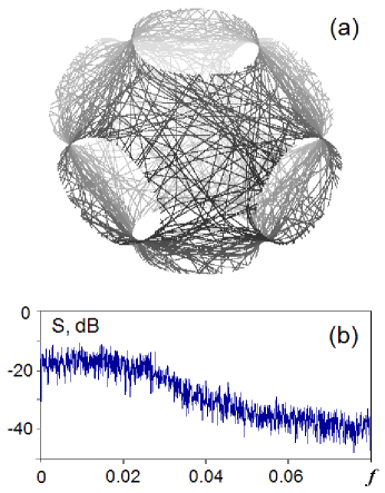
Figure 1: Typical trajectory of the system (4), (5) in a three-dimensional configuration space ($\theta_{1}$, $\theta_{2}$, $\theta_{3})$ (a) and power spectrum of the variable $\dot{\theta}_{1}$ for the motion with the kinetic energy $W$ = 0.03 (b). Plotting the diagram (a) the angular variables are related to the interval from 0 to 2$\pi$, i.e. it corresponds to the fundamental cell, which is repeated with period 2$\pi$ along each of the three coordinate axes.

In  17 a self-oscillating system was suggested, where the sustained dynamics corresponds approximately to the geodesic flow on the Schwarz surface; there the kinetic energy is not constant but undergoes some irregular fluctuations around a certain average level in the course of the dynamics in time. This system is based on three self-rotators, the elements whose state is defined by the angular variables $\theta_{1,2,3}$ and generalized velocities $\dot{\theta}_{1,2,3}$, and the steady motion of one element in isolation corresponds to the rotation in either direction with a certain constant angular velocity. The rotators are supposed to interact via the potential that is minimal under the condition (1). According to  17 , in a certain range of parameters the dynamics are hyperbolic, although for the modified system one should speak about self-oscillatory chaotic regimes corresponding to hyperbolic attractors rather then the Anosov dynamics. The purpose of this article is to propose an electronic circuit implementation of such system and to demonstrate its functioning as a generator of robust chaos.

For the construction of the electronic device the elements are required similar to rotators in mechanics. Namely, the state of the element has to be characterized by a generalized coordinate defined modulo 2$\pi$. An appropriate variable of such kind is a phase shift in the voltage controlled oscillator relative to a reference signal, like it is practiced in the phase-locked loops  21 .

Let us turn to the circuit diagram shown in Figure 2. The voltages $U_{1,2,3}$ are used to control the phases of the oscillators V1, V2, V3, so that the voltage outputs vary in time as $\sin(\omega t+\theta_{1,2,3})$, where the phases satisfy the equations $\dot{\theta}_{i}=kU_{i},\,\,\,i=1,2,3$, and $k$ is the coefficient characterizing the frequency control. The center frequency of the oscillators is determined by the bias provided by DC voltage source V4. The reference signal is generated by the AC voltage source V5.

Assuming the output voltages of the multipliers A1, A2, A3 to be $W_{1,2,3}$, for currents through the capacitors C1, C2, C3 we have $C\dot{U}_{i}+(R^{-1}-g)U_{i}+\alpha U_{i}+\beta U_{i}^{3}=R^{-1}W_{i}$, where $i$=1,2,3, $C$=C1=C2=C3, $R$=R10=R11=R12, and $I(U)=\alpha U+\beta U^{3}$ is the current-voltage characteristic of the nonlinear element composed of a pair of the diodes. The equations take into account the negative conductivity $g=R_{2}/R_{1}R_{3}=R_{5}/R_{4}R_{6}=R_{8}/R_{7}R_{9}$ introduced by the elements on the operation amplifiers U1, U2, U3. The voltages $W_{1,2,3}$ are obtained by multiplying the signals $\sin(\omega t+\theta_{1,2,3})\cos\omega t$ from outputs of A4, A5, A6 by an output signal $W$ of the inverting summing-integrating element containing the operational amplifier U4.

Input signals for the summing-integrating element are the output voltages of the multipliers A7, A8, A9, so, that with account of the leakage current through the resistor R16, we have $C_{0}\dot{W}+r^{-1}W=-R_{0}^{-1}[U_{1}\sin(\omega t+\theta_{1})+U_{2}\sin(\omega t+\theta_{2})+U_{3}\sin(\omega t+\theta_{3})]\cos\omega t$, where C₀=C4, $R_{0}$=R13=R14=R15, $r$=R16.

Using variables $\tau=t/\sqrt{4RCR_{0}C_{0}},\,\,\,u_{i}=2k\sqrt{RCR_{0}C_{0}}U_{i},\,\,\,w=2kR_{0}C_{0}W$ and parameters $\Omega=\sqrt{4RCR_{0}C_{0}}\omega,\,\,\,\mu=(gR-\alpha R-1)\sqrt{4R_{0}C_{0}/RC},\,\,\nu=\beta/\sqrt{4k^{4}RC^{3}R_{0}C_{0}},\,\,\,\gamma=\sqrt{4RCR_{0}/r^{2}C_{0}}$, we rewrite the equations in dimensionless form, where the dot means now the derivative over $\tau$:

$$\begin{array}[]{l}\dot{\theta}_{i}=u_{i},\,\,i=1,\,2,\,3,\\ \dot{u}_{i}=\mu u_{i}-\nu u_{i}^{3}+2w\sin(\Omega\tau+\theta_{i})\cos\Omega\tau,\\ \,\dot{w}=-\gamma w-2\sum\nolimits_{i=1}^{3}{u_{i}\sin(\Omega\tau+\theta_{i})\cos\Omega\tau}.\\ \end{array}$$ (6)

Non-trivial self-oscillatory behavior takes place at $\mu>0$; this parameter may be varied by simultaneous tuning the resistances R1, R4, R7.

Taking into account that $\Omega\gg 1$ one can simplify the equations assuming that $u_{i}$ and $w$ vary slowly on the high-frequency period. Namely, we perform averaging in the right-hand parts setting

$$\overline{\sin(\Omega\tau+\theta_{i})\cos\Omega\tau}=\textstyle{1\over 2}\sin\theta_{i}$$ (7)

and arrive at the equations

$$\begin{array}[]{l}\dot{\theta}_{i}=u_{i},\,\,\,\dot{u}_{i}=\mu u_{i}-\nu u_{i}^{3}+w\sin\theta_{i},\,\,\,\,i=1,\,\,2,\,\,3,\\ \dot{w}=-\gamma w-(u_{1}\sin\theta_{1}+u_{2}\sin\theta_{2}+u_{3}\sin\theta_{3}).\\ \end{array}$$ (8)

Finally, supposing $\gamma\ll 1$ we can neglect the respective term in the last equation and to integrate it with substitution of $u_{1,2,3}$ from the first equation; then we obtain $w\approx\cos\theta_{1}+\cos\theta_{2}+\cos\theta_{3}$, and the final result corresponds exactly to the equations of Ref.  17 :

$$\ddot{\theta}_{i}=\mu\dot{\theta}_{i}-\nu\dot{\theta}_{i}^{3}-(\cos\theta_{1}+\cos\theta_{2}+\cos\theta_{3})\sin\theta_{i},\,\,i=1,2,3.$$ (9)

Figure 3 shows a sample of the signal $U_{1}$ copied from the virtual oscilloscope screen when simulating the dynamics of the circuit in the NI Multisim software package, and the spectrum obtained with the virtual spectrum analyzer. Visually, the signal looks chaotic, without any apparent repetition of forms. Continuous spectrum indicates chaotic nature of the process. It is characterized by slow decrease of the spectral density with frequency and is of rather good quality in the sense of lack of pronounced peaks and dips.

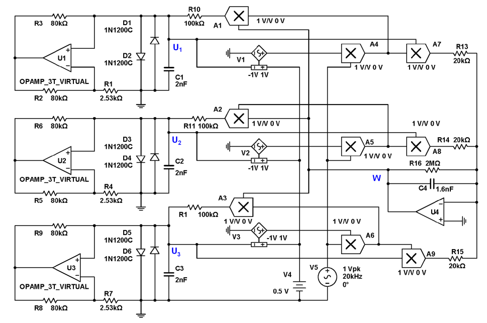
Figure 2: Circuit diagram of the chaos generator in the Multisim software package. The current-voltage characteristic of the nonlinear element with two parallel contrarily directed 1N1200C diodes is given approximately by the relation $I\approx\alpha U+\beta U^{3}$= 0.0039$U$+0.035$U^{3}$, where the current is expressed in amperes and the voltage – in volts. Coefficient of frequency control for V1, V2, V3 is $k$/2$\pi$=40 kHz/V.

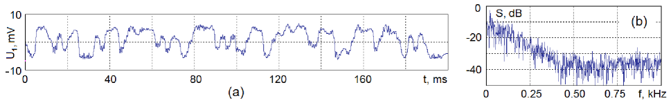
Figure 3: Voltage on capacitor C1 versus time in a sustained regime (a) and its power spectrum (b) as obtained by circuit simulation in Multisim.

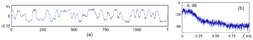
Figure 4: Time dependence (a) and spectrum (b) of the variable $u_{1}$ obtained from numerical integration of Eqs. (6).

In a frame of the circuit simulation it is difficult to explore some characteristics, such as Lyapunov exponents, therefore, we turn to comparison of the results with the model (6), for which the relevant analysis in the computations can be performed. Using the component nominals indicated in the circuit diagram of Fig.2 and applying the conversion formulas to the dimensionless quantities, we evaluate the parameters in the equations (6): $\mu=0.07497,\,\,\nu=1.73156,\,\,\gamma=0.05,\,\,\,\Omega=20.1062$. Figure 4 shows a plot of the dimensionless variable $u_{1}$ versus time obtained from the numerical integration of the equations (6) (a), and the Fourier spectrum (b). The scales on the axes are chosen to provide correspondence with Fig.3. Similar in form and characteristic scales are samples of time dependences and spectra obtained for the models (8) and (9).

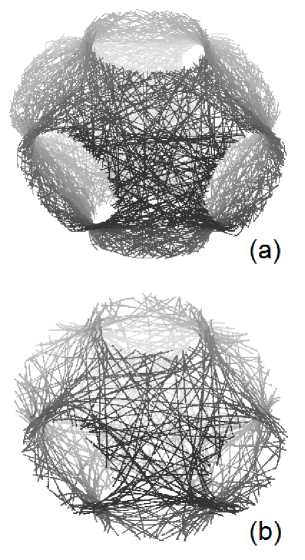
Figure 5: Trajectories in the three-dimensional space $(\theta_{1},\,\theta_{2},\,\theta_{3})$ for the model system (6) (a) and for the electronic device obtained from results of simulation in Multisim according to the method described in the text (b).

As one can see, the dynamics of the electronic device are similar to the original geodesic flow on the surface of negative curvature in the sense that the trajectories in the space of coordinate variables ($\theta_{1}$,$\theta_{2}$,$\theta_{3})$ are close to the Schwartz surface. This is illustrated in Fig.5, which shows a trajectory found by numerical integration of the equations for the model (6), and a diagram obtained from data of circuit simulation in Multisim. To plot the last one, the circuit was complemented by three special signal processing modules. The output signal of each of the voltage controlled oscillators subjected to multiplication by $\sin\omega t$ and $\cos\omega t$, and after filtration and separation of the low frequency components three pairs of the resulting signals ($x_{k}$, $y_{k})$, $k$=1,2,3 were recorded in a file for subsequent processing. According to the recorded data, at each time point three variables defined modulo 2$\pi$ are evaluated as $\theta_{k}=\arg(x_{k}+iy_{k})$, $k$=1,2,3, and respective points are plotted. These diagrams can be compared with Fig.1 for the geodesic flow on the surface of negative curvature. Figure 5 shows that the trajectory remains close to the Schwartz surface, though it is not located exactly on it; the pictures are ”fluffed” in the transverse direction. This effect becomes more pronounced with increasing parameter $\mu$, as we move away from the critical point of appearance of chaotic self-oscillations at $\mu$ = 0.

Figure 6 shows plots for all seven Lyapunov exponents calculated using Benettin algorithm  22 ; 23 ; 10 for the model (6) depending on the parameter $\mu$. In the presented range of $\mu$ we have one positive exponent, other two are close to zero, and the rest are negative. The dependence on the parameter is smooth, without pronounced peaks and dips, indicating the roughness of the chaotic attractor. Note that in  17 special calculations were carried out based on verification of the absence of tangencies between stable and unstable subspaces of perturbation vectors nearby a typical trajectory on the attractor for the model (9); it argues in favor of assumption of the hyperbolic nature of the dynamics for the system under consideration.

Particularly, at $\mu=0.07497$ the Lyapunov exponents of the attractor are $\lambda_{1}=0.1421\pm 0.0012$, $\lambda_{2}=0.0005\pm 0.0003$, $\lambda_{3}=0.0000\pm 0.0002$, $\lambda_{4}=-0.0547\pm 0.0006$, $\lambda_{5}=-0.0582\pm 0.0009$, $\lambda_{6}=-0.1382\pm 0.0004$, $\lambda_{7}=-0.1591\pm 0.0022$, where errors indicated are the standard deviations obtained under averaging data for 10² samples of duration $\tau$=5$\cdot$10⁴. The averaged dimensionless kinetic energy in this case according to the computations is $W=\textstyle{1\over 2}\overline{(u_{1}^{2}+u_{2}^{2}+u_{3}^{2})}\approx 0.0425$, so, for the comparable geodesic flow the Lyapunov exponents should be equal to $\pm 0.7\sqrt{W}\approx\pm 0.144$; that agrees well with $\lambda_{1}$ and $\lambda_{7}$ relating to the model (6).

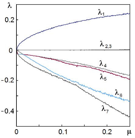
Figure 6: Lyapunov exponents of the system (6) depending on the parameter of supercriticality $\mu$.

Concluding, in this paper a construction of the electronic generator of rough chaos is proposed inspired by the problem of the geodesic flow on a surface of negative curvature, which implements hyperbolic dynamics of Anosov. An electron analog circuit simulation is provided in the NI Multisim software package. Also, the set of equations is derived to describe the system, and computational study of chaotic dynamics is performed on the base of these equations. In contrast to the previously considered electronic circuits with hyperbolic attractors  10 ; 11 ; 24 ; 25 , in this case the hyperbolic dynamics is characterized by higher degree of uniformity in expansion and compression for elements of the phase volume in the course of evolution in continuous time. Thus, the generated chaos has rather good quality of the power spectral density distributions.

Although the particular circuit described in the article operates in the low frequency range (kHz), it seems possible to implement similar devices at high frequencies as well.

Since the hyperbolic dynamics are characterized by roughness, or structural stability, as the mathematically proven attribute, it seems preferable for practical applications of chaos due to low sensitivity to parameter variations, various imperfections, noise, etc.

- (1) S. Smale, Bull. Amer. Math. Soc. (NS) 73, 747 (1967)
- (2) L. Shilnikov, Int. J. of Bifurcation and Chaos 7, 9 (1997) 1353.
- (3) D. V. Anosov, ed., Dynamical Systems 9: Dynamical Systems with Hyperbolic Behaviour, Encyclopaedia Math. Sci., Vol. 9 (Berlin: Springer, 1995).
- (4) A. Katok and B. Hasselblatt, Introduction to the Modern Theory of Dynamical Systems (Cambridge University Press, 1995).
- (5) Sinaĭ, Ya.G., Selected Translations, Selecta Math. Soviet. 1, 1 (1981) 100.
- (6) A.A. Andronov, A.A. Vitt, S.Ė. Khaĭkin, Theory of oscillators (Pergamon, 1966).
- (7) S. Banerjee, J. A. Yorke, and C. Grebogi, Physical Review Letters 80, 14 (1998) 3049.
- (8) Z. Elhadj and J.C. Sprott, Robust Chaos and Its Applications (World Scientific, Singapore, 2011).
- (9) A.S. Dmitriev, E.V. Efremova, N.A. Maksimov, A.I. Panas, Generation of chaos (Moscow: Technosfera, 2012) (Russian).
- (10) S.P. Kuznetsov, Phys. Uspekhi 54, 2 (2011) 119.
- (11) S.P. Kuznetsov, Hyperbolic Chaos: A Physicist’s View, Berlin: Springer, 2012.
- (12) D.V. Anosov, Trudy Mat. Inst. Steklov 90 (1967) 3 (Russian).
- (13) N.L. Balazs and A. Voros. Physics Reports 143, 3 (1986) 109.
- (14) W. H. III Meeks, J. Pérez, A survey on classical minimal surface theory. University Lecture Series, 60 (American Mathematical Society, 2012).
- (15) T.J. Hunt and R.S. MacKay, Nonlinearity 16 (2003) 1499.
- (16) S.P. Kuznetsov, Izv. Saratov. Univ. (N. S.), Ser. Fiz. 15, 2 (2015) 5 (Russian).
- (17) S.P. Kuznetsov, Regular and Chaotic Dynamics 20, 6 (2015) 649.
- (18) W.P. Thurston and J. R. Weeks, Sci. Am. 251, 1 (1984), 94.
- (19) V.V. Kozlov, Regular and Chaotic Dynamics 2, 1 (1997) 3 (Russian).
- (20) H. Goldstein, Ch.P. Jr. Poole, J.L. Safko, Classical Mechanics, 3rd ed. (Boston, Mass.: Addison-Wesley, 2001).
- (21) E. Best Roland, Phase-Locked Loops: Design, Simulation and Applications, 6th ed. (McGraw Hill, 2007).
- (22) G. Benettin, L. Galgani, A. Giorgilli and J.M. Strelcyn, Meccanica 15 (1980) 9.
- (23) H.G. Schuster and W. Just, Deterministic chaos: an introduction, 3rd ed. (Wiley-VCH, 2005).
- (24) O.B. Isaeva et al. Int. J. of Bifurcation and Chaos 25, 12 (2015) 1530033.
- (25) S.P. Kuznetsov, V.I. Ponomarenko, E.P. Seleznev, Izvestiya VUZ. Applied Nonlinear Dynamics (Saratov) 21, 5 (2013) 17 (Russian).