Relativistic two-body calculation of $b\bar{b}\,$-mesons radiative decays.

Abstract

This paper is a prosecution of a previous work where we presented a unified two-fermion covariant scheme which produced very precise results for the masses of light and heavy mesons. We extend the analysis to some radiative decays of mesons $\Upsilon,\,\chi_{b2}\,,h_{b}\,,\chi_{b1}\,,\chi_{b0}\,,\eta_{b}\,$ and we calculate their branching ratios and their widths. For most of them we can make a comparison with experimental data finding a good agreement.For the decays for which data are not available we compare ours with other recent theoretical previsions.

PACS numbers: 12.39.Pn, 03.65.Ge, 03.65.Pm, 14.40.Pq

I Introduction

Potential models have long been used to investigate the meson spectrum EGKKLY ; LSGI ; PotMod ; RR-BBD ; Gro . After the pioneering non relativistic work EGKKLY , it emerged with evidence that the relativity effects are important for the description of mesons Rich , both light and heavy, so that the following papers have eventually included relativistic corrections, either by perturbation methods or by covariant approaches in order to reach a reasonable precision LSGI ; RKMM . The chromodynamic interactions of heavy quarks through order $v^{2}/c^{2}$ were introduced in CasLep starting from a non relativistic treatment of QCD, defining an effective theory called NRQCD, which was used for lattice and continuum calculations LepThack ; BBL . This theory, together with a further effective theory derived from it, the potential non relativistic QCD or pNRQCD BPSV , is certainly one of the most diffused methods for calculating meson spectra and decays BEHV . The lattice techniques, on the other hand, have progressively improved up to the present day by including higher relativistic orders and QCD radiative effects, so that increasingly accurate determinations of hyperfine splittings have been calculated LW85 ; DDHH ; DDHHH ; LPR .

Other types of models move directly from a covariant formulation. A short list of up-to-date available relativistic or semi-relativistic models RK-CS ; Bra ; SeCe ; HC was discussed in our paper GSM . Starting from our previous results GS1 ; GS2 , we derived in GSM a completely covariant equation for two relativistic quarks of arbitrary mass interacting through the Cornell potential, with each of its two components taken in the vector or scalar coupling appropriate for the Dirac operators GS . Obviously the two spin-orbit couplings for the two quarks are completely included in our covariant approach so no problem concerning the reduced mass has to be posed. A first order correction to the potential was added by means of the Breit term. We then proved that our wave equation is able to provide a unified framework to investigate all ranges of meson masses. For heavier mesons the agreement with experimental data turned out to be really very precise up to the pair production threshold, not included in the Cornell potential. This gave suggestions for unknown spectroscopic classifications of some mesons and allowed us to obtain a good accuracy when calculating the masses of light mesons, for which potential models usually fail.

All the methods so far described are currently applied to the radiative meson decays, with the electromagnetic coupling generally taken in the dipole approximation (electric or magnetic according to the considered transitions). Sometimes the contributions due to the strong interactions are brought to bear to the calculation. In addition to the obvious comparison of the theoretical results with experimental data, in many papers previsions are also made on radiative transitions lacking direct data. In particular this is the case of the transitions of the recently observed mesons $h_{b}(1p)$ and $h_{b}(2p)$ decaying into $\eta_{b}(1s)$ and substantiating the evidence of $\eta_{b}(2s)$ Belle . The results of some recent papers using a semi-relativistic framework are found in GodMoa ; cinesi , those obtained by an effective potential are in cinese ; QCD based approaches are used in BJV ; BPV ; PS1 ; PS2 and lattice calculations of three-point matrix elements for radiative bottomonium decays are presented in LW . The width of the radiative decay of $\Upsilon(2s)$ into $\eta_{b}(1s)$ is given in HDDHHW . The agreement between theoretical and experimental widths is generally not as good as it is for the spectra, even when taking into account the large errors that affect the experimental data PDG .

The purpose of this paper is to use our two fermion covariant potential model GSM in order to calculate the purely radiative decays of $b\bar{b}$, still assuming the Cornell potential as a constitutive interaction for the mesons. The electromagnetic coupling for the composite two fermion system is then determined in analogy to the procedure established in BGS , where we calculated the hyperfine spacings for different hydrogenic atoms and the width of corresponding transitions, without invoking any other additional correction apart from the one given by the first order of the Breit term, that represents the spin-spin interaction responsible of the hyperfine splitting. The results we found are in extremely good agreement with the experimental data. It is therefore very tempting, if not compulsory, to have a look at the meson radiative decays by extending to mesons the treatment applied in BGS to atoms. We thus evaluate here the branching ratios and the widths of the measured radiative decays of $\Upsilon(3s),\,\chi_{b2}(2p),\,\chi_{b1}(2p),\,\chi_{b0}(2p),\,\Upsilon(2s)$ (see Tables III and IV) and we make previsions for some decays of $h_{b}(1p),\,h_{b}(2p),\,\chi_{b1}(2p)\Upsilon(2s),\,\Upsilon(1s)\,$ (see Table V) for which direct experimental data are not yet available. The results are rewarding, although we cannot expect to reach the same accuracy of the atomic calculations for several evident reasons. In the first place, the Cornell potential is itself an effective potential more suitable to the description of a stationary situation, such the calculation of the spectrum, as opposed to the atomic interaction which comes from a fundamental theory. Secondly, for atoms the fine structure coupling constant $\alpha_{{\rm{em}}}$ is the same for the Coulomb potential, the Breit spin-spin interaction and the decay process. This allows us to make a proper calculation of the first order corrections to the wave functions due to the Breit term as we did in BGS . These corrections turn out to be essential for getting very accurate values of both the hyperfine levels of different hydrogenic atoms and the decay widths. Without them the levels involved in hyperfine transitions would be degenerate and first order corrected wave functions are necessary to calculate the rate.

This is not the situation for meson radiative decays for which a rigorous perturbation expansion in the Breit term is not feasible. Indeed we have to remember that a remnant of the Breit correction is already present at the lowest order by means of the parameters entering the wave equation and its solutions.

          State Exp Num $({\texttt{1}}^{\texttt{1}}{\texttt{s}}_{\texttt{0}})~{}0^{+}(0^{-+})~{}\phantom{{}^{{}^{\displaystyle{i}}}}\!\!\eta_{b}$       9398.0$\pm$3.2 19390.39 $({\texttt{1}}^{\texttt{3}}{\texttt{s}}_{\texttt{1}})~{}0^{-}(1^{--})~{}\phantom{{}^{{}^{\displaystyle{i}}}}\!\!\varUpsilon$ 9460.30$\pm$.25 19466.10 $({\texttt{1}}^{\texttt{3}}{\texttt{p}}_{\texttt{0}})~{}0^{+}(0^{++})~{}\phantom{{}^{{}^{\displaystyle{i}}}}\!\!\chi_{b0}$ 9859.44$\pm$.73 19857.41 $({\texttt{1}}^{\texttt{3}}{\texttt{p}}_{\texttt{1}})~{}0^{+}(1^{++})~{}\phantom{{}^{{}^{\displaystyle{i}}}}\!\!\chi_{b1}$ 9892.78$\pm$.57 19886.70 $({\texttt{1}}^{\texttt{1}}{\texttt{p}}_{\texttt{1}})~{}0^{-}(1^{+-})~{}\phantom{{}^{{}^{\displaystyle{i}}}}\!\!h_{b}$ 9898.60$\pm$1.4 19895.35 $({\texttt{1}}^{\texttt{3}}{\texttt{p}}_{\texttt{2}})~{}0^{+}(2^{++})~{}\phantom{{}^{{}^{\displaystyle{i}}}}\!\!\chi_{b2}$ 9912.21$\pm$.57 19908.14 $({\texttt{2}}^{\texttt{1}}{\texttt{s}}_{\texttt{0}})~{}0^{+}(0^{-+})~{}\phantom{{}^{{}^{\displaystyle{i}}}}\!\!\eta_{b}$ M9974.0$\pm$4.4${}^{\,(\ast)}$ .9971.14 $({\texttt{2}}^{\texttt{3}}{\texttt{s}}_{\texttt{1}})~{}0^{-}(1^{--})~{}\phantom{{}^{{}^{\displaystyle{i}}}}\!\!\varUpsilon$ 10023.26$\pm$.0003 10009.04 $({\texttt{2}}^{\texttt{3}}{\texttt{p}}_{\texttt{0}})~{}0^{+}(0^{++})~{}\phantom{{}^{{}^{\displaystyle{i}}}}\!\!\chi_{b0}$ 10232.50$\pm$.0009 10232.36 $({\texttt{2}}^{\texttt{3}}{\texttt{p}}_{\texttt{1}})~{}0^{+}(1^{++})~{}\phantom{{}^{{}^{\displaystyle{i}}}}\!\!\chi_{b1}$ 10255.46$\pm$.0005 10256.58 $({\texttt{2}}^{\texttt{1}}{\texttt{p}}_{\texttt{1}})~{}0^{-}(1^{+-})~{}\phantom{{}^{{}^{\displaystyle{i}}}}\!\!h_{b}$ 10259.8$\pm$1.6 110263.62 $({\texttt{2}}^{\texttt{3}}{\texttt{p}}_{\texttt{2}})~{}0^{+}(2^{++})~{}\phantom{{}^{{}^{\displaystyle{i}}}}\!\!\chi_{b2}$ 10268.65$\pm$.0007 10274.26 $({\texttt{3}}^{\texttt{3}}{\texttt{s}}_{\texttt{1}})~{}0^{-}(1^{--})~{}\phantom{{}^{{}^{\displaystyle{i}}}}\!\!\varUpsilon$ 10355.20$\pm$.0005 i10364.52

Table 1: The $b\bar{b}$ levels in MeV. First column: term symbol, $I^{G}(J^{PC})$ numbers , particle name. $\sigma$=1.111 GeV/fm, $\alpha$=0.3272, $m_{b}$=4725.5 MeV. Experimental data are taken from PDG . Our values can be compared with those obtained by different approaches, reported in cinesi . ${}^{\,(\ast)}$ see Nota1 .

This happens because in most quarkonium models, as in ours, the values assumed for both $\alpha_{{\rm{QCD}}}$ and for the string tension $\sigma$ are obtained from a fit of the experimental meson spectrum GSM , calculated by taking into account the first order of the Breit correction. In Table I here below we report the masses of the mesons we will consider later on Nota1 . On the other hand, in Table II we show the actually very different influence of the Breit term on the different states.

    $~{}\eta_{b}(1s)~{}~{}~{}$ $\Upsilon_{b}(1s)~{}~{}~{}$ $\chi_{b0}(1p)~{}~{}~{}$ $\chi_{b1}(1p)~{}~{}~{}$ $h_{b}(1p)~{}~{}~{}$ $\chi_{b2}(1p)~{}$  -92.13 -18.09 -44.3 -19.98 -15.95 -7.51 

Table 2: The Breit corrections in MeV for the lowest states.

Due to the structure of the transition rate given in the following equation (4), if we use the physical (i.e. Breit corrected) value for the transition frequency it seems reasonable to take the corresponding spinors at the lowest perturbation order. However for the states with $j=0$, namely $\eta_{b}$ and $\chi_{b0}$, the hyperfine shift is maximal and considerably larger than for the other states of their respective multiplets. These states are connected by a parity transformation and in our model they are structurally distinguished from the other components of the respective multiplets since they are determined by a second order differential system instead of by a fourth order one. Moreover the inclusion of the first order corrections in their wave functions makes a really great improvement on the results of the decay transition rate. Still in the context of radiative meson decays, an analogous situation was met in Gro for the relativistic corrections in $v^{4}/c^{4}$ “retained in the calculation of those rates where those terms make a substantial difference” (see Gro , note 18). Therefore we shall assume unperturbed wave functions for all the $j\neq 0$ states and first order corrected wave functions for all the $j=0$ states. In the last section the numerical method of calculating the corrections to levels and states will be recalled.

We now give a sketchy summary of what follows. In the next section we recall the general formulae of our method: we refer for details to our papers GSM ; BGS . In order to have an idea of the properties of the eigenfunctions, we present a plot of the radial probability density of the states. In section III we discuss some numerical aspects, describing the way our spinors are calculated and giving some details on the numerical precision; we will then present the results and make some concluding remarks. Our approach is conceptually simple; it is completely covariant, so that it includes all the relativistic effects; it contains the Breit interaction responsible for the hyperfine splittings. It has a general application to potential models and drastically limits the number of corrections needed about in order to achieve agreement with experimental data. It is also rather manageable on the side of explicit computations in a combined environment of numerical methods and computer algebra. This is indeed the method we have used for getting the results we have given. The expressions we have used and the equations we have solved can be deduced, with some work, from our papers GSM ; BGS by implementing the general relations to the present case which appears simpler because of the equality of the two quark masses. However we believe it to be useful for the reader if in Appendix we revisit our method for the $b\bar{b}$ systems, cutting the exposition down to the bone and specifying only those elements necessary for the present calculations of the radiative decay widths. This, in addition, gives us the possibility of some further observations of a more technical character.

II The transition probabilities

From GSM we have that the two-body relativistic wave equation for $b\bar{b}$, with eigenvalue $\lambda$, reads

$$\!\!\!\Bigl{[}\,\Bigl{(}{\gamma}^{0}_{(1)}{\gamma_{(1)}}_{a}-{\gamma}^{0}_{(2)}{\gamma_{(2)}}_{a}\Bigr{)}q_{a}+\frac{1}{2}\Bigl{(}{\gamma}^{0}_{(1)}\!+\!{\gamma}^{0}_{(2)}\Bigr{)}\Bigl{(}2m_{b}+\sigma r\Bigr{)}-\vrule height=11.99998pt,width=0.0pt,depth=11.99998pt$$ (1)

$$\phantom{XXXXX}\Bigl{(}\lambda+\frac{b}{r}\Bigr{)}+V_{B}(r)\,\Bigr{]}\,\Psi(\vec{r})=0.$$ (2)

where $\Psi(\vec{r})$ is a 16-component spinor obtained by reordering the tensor product of the two quarks so as to collect singlets and triplets for the different eigenvalues of the mass GS1 ; BGS , ${\gamma}^{0}_{(i)},{\gamma_{(i)}}_{a}$ are the $\gamma$ matrices acting on the space of the quark and anti-quark fermion and $b=(4/3)\,\alpha_{QCD}$. The vector and scalar parts of the Cornell potential respectively give the $(\lambda+b/r)$ and $(2m_{b}+\sigma r)$ terms. Finally the Breit potential $V_{B}(r)$ has the form

$$V_{B}(r)=\frac{b}{2r}\,{\gamma}^{0}_{(1)}{\gamma_{(1)}}_{a}{\gamma}^{0}_{(2)}{\gamma_{(2)}}_{b}\Bigl{(}\delta_{ab}\!+\!\frac{r_{a}r_{b}}{r^{2}}\Bigr{)}$$ (3)

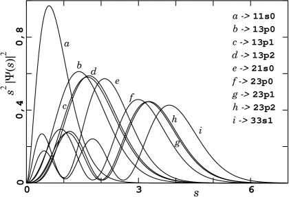
Figure 1: The normalized densities of the states involved in the $\Upsilon(3)$ decay times the measure factor in the dimensionless coordinate $s$ defined in Appendix.

As explained in GSM , when we calculate the meson spectrum the wave equation reduces to a system of four linear differential equations (see also GS1 ; GS2 for further details).

We choose the reference frame with vanishing total momentum $\emph{{P}}_{i}$ and we use the global/relative canonical coordinates $(Z,\emph{{r}})$ (see Appendix A of BGS ). We factorize the wave functions of initial and final bottomonium states, normalized in a box of volume $V$, into

$$\Psi_{\ell}(Z,\emph{{r}})=V^{-1/2}\,{e^{-iP_{\ell}\cdot Z}}\,\psi_{\ell}(\emph{{r}})\,,\quad\ell=i,f\,$$

where $\psi_{i}(\emph{{r}})$ and $\psi_{f}(\emph{{r}})$ are the 16-component spinors corresponding to initial and final energies, angular momenta and parities. The Breit term (3) will always be considered a first order perturbation term. As previously said, when necessary we will consider wave functions represented by the sum of a lowest order contribution given by the exact eigenfunction of equation (2) with $V_{B}(r)=0$ and a first order correction generated by $V_{B}(r)$ itself. The general systems of equations for the case of mesons formed by quarks with possibly different masses is presented in GSM : we report in the Appendix the systems for the $b\bar{b}$ case, not explicitly written in our previous papers. In BGS it was shown that the electromagnetic coupling for the fermion - anti-fermion bound system is introduced by means of the interaction Hamiltonian

$$H_{\mathrm{int}}=-e_{b}\,\Bigl{(}\,\bm{\alpha}_{(1)}\!\cdot\!\emph{{A}}^{{(1)}}-\bm{\alpha}_{(2)}\!\cdot\!\emph{{A}}^{{(2)}}\,\Bigr{)}$$

where $e_{b}=(1/3)\,e$ is the bottom charge, $e$ being the electron charge. Here $~{}\bm{\alpha}_{(i)}$ is the vector of the $\alpha$-matrices for the $i$-th fermion space, $\emph{{A}}^{{(i)}}$ is the wave function of a photon with 4-momentum $k$ and polarization ${\bm{\epsilon}}_{\sigma}$ in the Coulomb gauge Landau ,

$${\bm{A}}(k,\sigma)=\frac{\sqrt{4\pi}}{\sqrt{2\omega\,V}}\,\,{\bm{\epsilon}}_{\sigma}\,\,e^{\displaystyle-i\,k_{\mu}x^{\mu}}\,,$$

calculated at the coordinate $x=x_{(i)}$, where $\omega=k_{0}$ is the photon frequency. For equal fermion masses, the standard calculation for the first perturbation order of the $S$-matrix element at fixed initial and final states gives

$$S_{fi}=-ie_{b}\,\frac{(2\pi)^{4}}{\sqrt{2\omega V}}\,\frac{\sqrt{4\pi}}{\sqrt{V^{2}}}\,\delta^{4}(P_{f}+k-P_{i})\,(\bm{\epsilon}_{\sigma}^{*}\!\cdot\!\bm{M}_{fi})~{}~{}~{}~{}~{}$$

where

$$\bm{M}_{fi}=\int d^{3}\emph{{r}}\,\,\psi^{*}_{f}(\emph{{r}})\,\Bigl{(}\,\widetilde{\bm{\alpha}}_{(1)}\,e^{-\frac{i}{2}{\emph{{k}}}\,\cdot\!\!\!\!{\emph{ { r }}}}-\widetilde{\bm{\alpha}}_{(2)}\,e^{\frac{i}{2}{\emph{{k}}}\,\cdot\!\!\!\!{\emph{ { r }}}}\Bigr{)}\,\psi_{i}(\emph{{r}})\,.\vrule height=8.00003pt,width=0.0pt,depth=8.00003pt$$

Here $\widetilde{\bm{\alpha}}_{(j)}$ are the transformed matrices in the basis of the spinors with reordered components above mentioned. The $\delta^{4}$-function gives the conservation of the global 4-momentum

$$P^{\mu}_{i}=P^{\mu}_{f}+k^{\mu}$$

and contains the recoil of the meson due to the radiation emission. Using the explicit form of the spinors obtained by the diagonalization of total angular momentum and parity (see Appendix), the integrals over the angular variables can be analytically calculated, without any approximation on the exponential, in terms of elementary functions that correspond to the lowest order Bessel functions appearing in the usual series expansions. The radial integrals are then calculated numerically for all the allowed transitions as described in more detail in the next section.

Summing over the polarizations and the possible final states and averaging over the initial states, the differential transition rate therefore reads

$$dw=\frac{e_{b}^{2}}{2\pi\omega}\,\delta^{4}(P_{f}+k-P_{i})\sum\,\frac{|\bm{\epsilon}_{\sigma}^{*}\!\cdot\!\!\emph{{M}}_{fi}|^{2}}{2j_{i}+1}\,\,{d^{3}\!\!\emph{ {k}}}\,\,{d^{3}\emph{{P}}_{f}}\vrule height=11.99998pt,width=0.0pt,depth=11.99998pt$$

As $\int{d^{3}\emph{{P}}}/{2P^{0}}=\int d^{4}{P}\,\theta(P^{0})\,\delta(P^{2}-\lambda^{2})\,,$ integrating over the final global momentum we get

$$\frac{dw}{d\omega\,d\Omega_{n}}\!=\!\frac{e_{b}^{2}\,\omega}{2\pi\lambda_{i}}\,(\lambda_{i}-\omega)\,\delta\Bigl{(}\omega-\frac{\lambda_{i}^{2}-\lambda_{f}^{2}}{2\lambda_{i}}\Bigr{)}\sum\,\frac{|\bm{\epsilon}_{\sigma}^{*}\!\cdot\!\!\emph{{M}}_{fi}|^{2}}{2j_{i}+1}$$

where $d\Omega_{n}$ is the unit solid angle in the direction $\emph{{n}}=\emph{{k}}/|\emph{{k}}|$. Reinserting the $\hbar$ and $c$ factors, the final integration over the solid angle gives the total transition rate

$$w=\frac{4}{3}\,\frac{e_{b}^{2}}{\hbar c}\,\,\omega_{fi}\,\,\Lambda_{fi}^{2}\,\sum\,\frac{|\bm{\epsilon}_{\sigma}^{*}\!\cdot\!\!\emph{{M}}_{fi}|^{2}}{2j_{i}+1}$$ (4)

while

$$\omega_{fi}=\frac{c}{\hbar}\,\,\frac{\lambda_{i}+\lambda_{f}}{2\lambda_{i}}\,(\lambda_{i}-\lambda_{f})$$

is the frequency of the emitted photon that completely includes the recoil. Finally

$$\Lambda_{fi}^{2}=\frac{\lambda^{2}_{i}+\lambda^{2}_{f}}{2\lambda^{2}_{i}}$$

is the relativistic correction factor coming from kinematics. This is not very far from unity but for the transitions between states with large mass difference.

III NUMERICAL RESULTS AND CONCLUSIONS

As extensively described in GSM ; BGS , the levels and the eigenstates are obtained by a numerical solution of the singular boundary value problem (BVP) posed by the Hamiltonian (2) acting on 16-component spinors involving eight radial function coefficients $\{a_{i}(r),b_{i}(r),c_{i}(r),d_{i}(r)\}_{i=0,1}$. The symmetries of the problem imply four algebraic relations, so that the previous radial functions can be expressed in terms of only four unknown functions $\{u_{i}(r)\}_{i=1,4}$ and the the BVP reduces to a $4\times 4$ linear differential system for each parity. As stated above, for the $j=0$ states, the $4\times 4$ system actually reduces to a $2\times 2$ one. In the Appendix we specify the matrix elements of the reduced differential systems and we give the explicit expression of the $a_{i},b_{i},c_{i},d_{i}$ in terms of the $u_{k}$. We also add some comments on the $P$- and $PC$-transformations.

      XXXXXXXXBranching Ratios Theor ExpX. $\Upsilon(3s)\rightarrow\gamma\chi_{b1}(2p)/\Upsilon(3s)\rightarrow\gamma\chi_{b2}(2p)~{}~{}$ .812 .96$\pm$.21 $\Upsilon(3s)\rightarrow\gamma\chi_{b0}(2p)/\Upsilon(3s)\rightarrow\gamma\chi_{b2}(2p)~{}~{}$ .433 .45$\pm$.10 $\Upsilon(3s)\rightarrow\gamma\eta_{b}(2s)/\Upsilon(3s)\rightarrow\gamma\chi_{b2}(2p)~{}~{}$ .002 <.005 $\Upsilon(3s)\rightarrow\gamma\chi_{b2}(1p)/\Upsilon(3s)\rightarrow\gamma\chi_{b2}(2p)~{}~{}$ .042 .075$\pm$.019 $\Upsilon(3s)\rightarrow\gamma\chi_{b1}(1p)/\Upsilon(3s)\rightarrow\gamma\chi_{b2}(2p)~{}~{}$ .010 .007$\pm$.005 $\Upsilon(3s)\rightarrow\gamma\chi_{b0}(1p)/\Upsilon(3s)\rightarrow\gamma\chi_{b2}(2p)~{}~{}$ .010 .021$\pm$.006 $\Upsilon(3s)\rightarrow\gamma\eta_{b}(1s)/\Upsilon(3s)\rightarrow\gamma\chi_{b2}(2p)~{}~{}$ .003 .004$\pm$.001 $\Upsilon(2s)\rightarrow\gamma\chi_{b1}(1p)/\Upsilon(2s)\rightarrow\gamma\chi_{b2}(1p)~{}~{}$ .812 .96$\pm$.10 $\Upsilon(2s)\rightarrow\gamma\chi_{b0}(1p)/\Upsilon(2s)\rightarrow\gamma\chi_{b2}(1p)~{}~{}$ .410 .53$\pm$.08 $\Upsilon(2s)\rightarrow\gamma\eta_{b}(1s)/\Upsilon(2s)\rightarrow\gamma\chi_{b2}(1p)~{}~{}$ .006 .006$\pm$.002 $\chi_{b2}(2p)\rightarrow\gamma\Upsilon(1s)/\chi_{b2}(2p)\rightarrow\gamma\Upsilon(2s)~{}~{}$ .55 .66$\pm$.23 $\chi_{b1}(2p)\rightarrow\gamma\Upsilon(1s)/\chi_{b1}(2p)\rightarrow\gamma\Upsilon(2s)~{}~{}$ .46 .46$\pm$.08 $\chi_{b0}(2p)\rightarrow\gamma\Upsilon(1s)/\chi_{b0}(2p)\rightarrow\gamma\Upsilon(2s)~{}~{}$ .13 (.20$\pm$.20)^(∗)

Table 3: Comparison of our calculated branching ratios of the radiative decays with experimental data. The experimental errors have been linearly combined. ^(∗)This case is not very meaningful due to the large error by which it is affected.

        Decay xxTheor ExpXX $\Upsilon(3s)\rightarrow\gamma\chi_{b2}(2p)~{}~{}$    3.51   2.70$\pm$0.57 $\Upsilon(3s)\rightarrow\gamma\chi_{b1}(2p)~{}~{}$    2.85   2.58$\pm$0.48 $\Upsilon(3s)\rightarrow\gamma\chi_{b0}(2p)~{}~{}$    1.52   1.21$\pm$0.23 $\Upsilon(3s)\rightarrow\gamma\eta_{b}(2s)~{}~{}$    0.006   < 0.013 $\Upsilon(3s)\rightarrow\gamma\chi_{b2}(1p)~{}~{}$    0.149   0.204$\pm$0.045 $\Upsilon(3s)\rightarrow\gamma\chi_{b1}(1p)~{}~{}$    0.036   0.019$\pm$0.012 $\Upsilon(3s)\rightarrow\gamma\chi_{b0}(1p)~{}~{}$    0.032    0.056$\pm$0.013 $\Upsilon(3s)\rightarrow\gamma\eta_{b}(1s)~{}~{}$    0.009   0.011$\pm$0.003 $\Upsilon(2s)\rightarrow\gamma\chi_{b2}(1p)~{}~{}$    2.13   2.30$\pm$0.20 $\Upsilon(2s)\rightarrow\gamma\chi_{b1}(1p)~{}~{}$    1.73   2.22$\pm$0.21 $\Upsilon(2s)\rightarrow\gamma\chi_{b0}(1p)~{}~{}$    0.87    1.22$\pm$0.15 $\Upsilon(2s)\rightarrow\gamma\eta_{b}(1s)~{}~{}$    0.013   0.013$\pm$0.04 $\chi_{b2}(2p)\rightarrow\gamma\Upsilon(2s)~{}~{}$    18.77   15.10$\pm$5.60 $\chi_{b2}(2p)\rightarrow\gamma\Upsilon(1s)~{}~{}$    10.27   9.80$\pm$2.30 $\chi_{b1}(2p)\rightarrow\gamma\Upsilon(2s)~{}~{}$    16.80   14.40$\pm$5.00 $\chi_{b1}(2p)\rightarrow\gamma\Upsilon(1s)~{}~{}$    7.68   8.96$\pm$2.24 $\chi_{b0}(2p)\rightarrow\gamma\Upsilon(2s)~{}~{}$    11.77   - $\chi_{b0}(2p)\rightarrow\gamma\Upsilon(1s)~{}~{}$    1.49   - $\chi_{b2}(1p)\rightarrow\gamma\Upsilon(1s)~{}~{}$    33.73   - $\chi_{b1}(1p)\rightarrow\gamma\Upsilon(1s)~{}~{}$    29.48   - $\chi_{b0}(1p)\rightarrow\gamma\Upsilon(1s)~{}~{}$    19.65   -

Table 4: Values in keV of the theoretical and experimental widths of radiative decays of $\Upsilon(3s),\,\chi_{b2}(2p)\,,\chi_{b1}(2p)\,,\chi_{b0}(2p)\,,\Upsilon(2s)$.

Moreover, the corrections due to the Breit term (3) are calculated by solving the BVP for $\varepsilon V_{B}(r)$ and taking the first order expansion in $\varepsilon$ both for levels and spinors normalized to unity. Due to the value of the bottom mass, the parameters entering the BVP are such that the solutions can be expressed directly in terms of Padé approximants, so that we get a complete control of the numerical error. The Padé we have calculated are of order [260,260] and since the arithmetical precision has also been taken with a sufficiently large number of digits, our numerical errors can safely be assumed to be vanishing. Just to have a consistency test of our eigenfunctions with the covariant framework in which they are determined, we have calculated some estimates of the average meson radii and quark velocity. For the radii we have seen a monotonic increase with mass, from $0.156\,\,$fm of the $\eta_{b}(1s)$ to $0.609\,\,$fm of $\Upsilon(3p)$. The estimate of the quark velocity has been approximated by $\beta\simeq(\langle{\bm{q}}^{2}\rangle/(m^{2}c^{2}+\langle{\bm{q}}^{2}\rangle))^{1/2}$, where $q=(p_{1}-p_{2})/2$ is the conjugate relative momentum of the two fermions GSM ; BGS and $\langle{\bm{q}}^{2}\rangle$ has been taken as the he average of $\,-\hbar^{2}\,{\bm{\nabla}}^{2}_{r}\,$ over the corresponding state. Averaging then over all the states we have found a $\beta\simeq 0.29$ in good agreement with the estimate of PS2 . Such a value, in our opinion, strengthens the idea that a completely relativistic treatment is appropriate. Finally we have calculated the average values of the orbital angular momentum from the radial part of the Laplace operator and we have found values no larger than 0.115 for $s$-states and values between 0.976 and 1.045 for $p$-states.

In Table III we present our results for ‘relative’ branching ratios of bottomonium radiative decays, namely for branching ratios not using the total width of the decaying particle and we make a comparison with experimental data whose errors have been linearly combined. It appears that the agreement between theoretical and experimental data is very good for most of the decays and that the worst results are different for a factor not greater than 1.5.

In the second column of Table IV we report the values in keV we have calculated for the $b\bar{b}$ mesons radiative decays. We get from PDG the total widths $\Gamma_{\Upsilon(3s)}=20.32\pm 1.85\,\,$keV, $\Gamma_{\Upsilon(2s)}=31.98\pm 2.63\,\,$keV, while the total widths of $\Gamma_{\chi_{b2}(2p)}=138.\pm 19.\,\,$keV and $\Gamma_{\chi_{b1}(2p)}=96.\pm 16.\,\,$keV are taken from Caw . Again we have assumed a linear composition of the errors of the experimental data. The agreement is again very good even for the decays involving the $\eta_{b}$ and the $\chi_{b0}$ states. Tables of the results for the decay withs obtained by several different approaches can be found in cinesi .

In Table V we give the results of our previsions in comparison with those of References cinesi and PS2 .

Appendix

The general notations, the derivation of the wave equation and the proof of many of its properties (variables, covariance and so on) have been given in GS1 ; GS2 ; GSM . The eigenfunctions of the Hamiltonian (2), obtained by coupling two Dirac equations, are 16-dimensional spinors.

If $m_{b}$ is the bottom mass, we introduce the dimensionless variables $\Omega,\,w,\,s$ by

$$\!\!\!\sigma=m_{b}^{2}\,\Omega^{\frac{3}{2}},~{}~{}\lambda=m_{b}\,(2+\Omega w),~{}~{}r=m_{b}^{-1}\,\Omega^{-\frac{1}{2}}\,s,$$

$\blacktriangleright$ The parity operator $P$ is given by the inner parity – which is the reordered $\gamma_{0}\otimes\gamma_{0}$ – combined with the change $\bm{r}\rightarrow-\bm{r}$ times a global arbitrary phase. In our previous papers dealing with atomic states we had called “even” or “odd” the states with eigenvalues of $P$ equal to ${(-)}^{j}$ or ${(-)}^{j+1}$ respectively, choosing the arbitrary phase equal to unity. With such a choice the ground state of an atomic system has the $P$ eigenvalue equal to unity. We maintain this terminology but we observe that we have to choose the global phase equal to -1 in order to agree with the usual meson classification scheme.

        Decay Ours Ref[28] Ref[23]   $h_{b}(2p)\rightarrow\gamma\eta_{b}(2s)~{}~{}$ 20681 17600 16600 $h_{b}(2p)\rightarrow\gamma\eta_{b}(1s)~{}~{}$ 16884 14900 17500 $\Upsilon(2s)\rightarrow\gamma\eta_{b}(2s)~{}~{}$ 0.369 0.58 0.59    $\eta_{b}(2s)\rightarrow\gamma\Upsilon(1s)~{}~{}$ 65.41 45 64    $\chi_{b2}(1p)\rightarrow\gamma h_{b}(1p)~{}~{}$ 0.015 0.089 $\chi_{b2}(1p)\rightarrow\gamma\Upsilon(1s)$ 33731 39150 31800 $h_{b}(1p)\rightarrow\gamma\chi_{b1}(1p)~{}~{}$ 0.050 0.012 0.0094 $h_{b}(1p)\rightarrow\gamma\chi_{b0}(1p)~{}~{}$ 0.124 0.86 0.90 $h_{b}(1p)\rightarrow\gamma\eta_{b}(1s)~{}~{}$ 39318 43660 35800 $\Upsilon(1s)\rightarrow\gamma\eta_{b}(1s)~{}~{}$ 3.101^∗ 9.34   10   

Table 5: Comparison of the previsions for the theoretical widths of some radiative decays of $\chi_{b2},\,h_{b},\,\chi_{b1},\,\chi_{b0}\,\,{\mathrm{and}}\,\,\Upsilon$. Units are eV. ^∗ This value is in agreement with the value (3.6$\pm$2.9) eV of BPV .

After diagonalization of angular momentum and parity the components of the general reordered spinor we have called “even” are GS1 ; BGS

$$\psi_{+\,0}^{(M)}=Y^{j}_{m}(\theta,\,\phi)\,{a_{0}}(s)~{}~{}~{}~{}~{}~{}~{}~{}~{}\,\vrule height=11.99998pt,width=0.0pt,depth=11.99998pt$$ (5)

$$\psi_{+\,1_{+}}^{(M)}=-{\displaystyle\frac{\sqrt{j-m+1}\sqrt{j+m}}{\sqrt{2\,j}\sqrt{j+1}}}\,Y^{j}_{m-1}(\theta,\,\phi)\,{b_{0}}(s)\vrule height=11.99998pt,width=0.0pt,depth=11.99998pt$$ (6)

$$\psi_{+\,1_{0}}^{(M)}={\displaystyle\frac{m}{\sqrt{j}\,\sqrt{1+j}}}\,Y^{j}_{m}(\theta,\,\phi)\,\,{b_{0}}(s)\vrule height=11.99998pt,width=0.0pt,depth=11.99998pt$$ (7)

$$\psi_{+\,1_{-}}^{(M)}={\displaystyle\frac{\sqrt{j-m}\,\sqrt{j+m+1}}{\sqrt{2\,j}\sqrt{j+1}}}\,Y^{j}_{m+1}(\theta,\,\phi)\,{b_{0}}(s)\vrule height=11.99998pt,width=0.0pt,depth=11.99998pt$$

$$\psi_{+\,0}^{(-M)}=Y^{j}_{m}(\theta,\,\phi)\,{a_{1}}(s)\vrule height=11.99998pt,width=0.0pt,depth=11.99998pt$$ (8)

$$\psi_{+\,1_{+}}^{(-M)}=-{\displaystyle\frac{\sqrt{j-m+1}\sqrt{j+m}}{\sqrt{2\,j}\sqrt{j+1}}}\,Y^{j}_{m-1}(\theta,\phi)\,{b_{1}}(s)\vrule height=11.99998pt,width=0.0pt,depth=11.99998pt$$ (9)

$$\psi_{+\,1_{0}}^{(-M)}={\displaystyle\frac{m}{\sqrt{j}\,\sqrt{1+j}}}\,Y^{j}_{m}(\theta,\,\phi)\,{b_{1}}(s)\vrule height=11.99998pt,width=0.0pt,depth=11.99998pt$$ (10)

$$\psi_{+\,1_{-}}^{(-M)}={\displaystyle\frac{\sqrt{j-m}\sqrt{j+m+1}}{\sqrt{2\,j}\sqrt{j+1}}}\,Y^{j}_{m+1}(\theta,\phi)\,{b_{1}}(s)\vrule height=11.99998pt,width=0.0pt,depth=11.99998pt$$

$$\psi_{+\,0}^{(-\mu)}=0\vrule height=11.99998pt,width=0.0pt,depth=11.99998pt$$ (11)

$$\psi_{+\,1_{+}}^{(-\mu)}={\displaystyle\frac{\sqrt{j+m-1}\,\sqrt{j+m}}{\sqrt{2\,j}\,\sqrt{2\,j-1}}}\,Y^{j-1}_{m-1}(\theta,\,\phi)\,{c_{0}}(s)+\vrule height=11.99998pt,width=0.0pt,depth=11.99998pt$$ (12)

$$\phantom{\psi_{+\,1_{+}}^{(-\mu)}=X}{\displaystyle\frac{\sqrt{j-m+1}\,\sqrt{j-m+2}}{\sqrt{2\,j+2}\,\sqrt{2\,j+3}}}\,Y^{j+1}_{m-1}(\theta,\,\phi)\,{d_{0}}(s)\vrule height=11.99998pt,width=0.0pt,depth=11.99998pt$$ (13)

$$\psi_{+\,1_{0}}^{(-\mu)}={\displaystyle\frac{\sqrt{j-m}\,\sqrt{j+m}}{\sqrt{j}\,\sqrt{2\,j-1}}}\,Y^{j-1}_{m}(\theta,\,\phi)\,{c_{0}}(s)-\vrule height=11.99998pt,width=0.0pt,depth=11.99998pt$$ (14)

$$\phantom{\psi_{+\,1_{0}}^{(-\mu)}=X}{\displaystyle\frac{\sqrt{j-m+1}\,\sqrt{j+m+1}}{\sqrt{1+j}\,\sqrt{2\,j+3}}}\,Y^{j+1}_{m}(\theta,\,\phi)\,{d_{0}}(s)\vrule height=11.99998pt,width=0.0pt,depth=11.99998pt$$ (15)

$$\psi_{+\,1_{-}}^{(-\mu)}={\displaystyle\frac{\sqrt{j-m-1}\,\sqrt{j-m}}{\sqrt{2\,j}\,\sqrt{2\,j-1}}}\,Y^{j-1}_{m+1}(\theta,\,\phi)\,{c_{0}}(s)+\vrule height=11.99998pt,width=0.0pt,depth=11.99998pt$$ (16)

$$\phantom{\psi_{+\,1_{-}}^{(-\mu)}=X}{\displaystyle\frac{\sqrt{j+m+1}\,\sqrt{j+m+2}}{\sqrt{2\,j+2}\,\sqrt{2\,j+3}}}\,Y^{j+1}_{m+1}(\theta,\,\phi)\,{d_{0}}(s)\vrule height=11.99998pt,width=0.0pt,depth=11.99998pt$$

$$\psi_{+\,0}^{(\mu)}=0\vrule height=11.99998pt,width=0.0pt,depth=11.99998pt$$ (17)

$$\psi_{+\,1_{+}}^{(\mu)}={\displaystyle\frac{\sqrt{j+m-1}\,\sqrt{j+m}}{\sqrt{2\,j}\,\sqrt{2\,j-1}}}\,Y^{j-1}_{m-1}(\theta,\,\phi)\,{c_{1}}(s)+\vrule height=11.99998pt,width=0.0pt,depth=11.99998pt$$ (18)

$$\phantom{\psi_{+\,1_{+}}^{(-\mu)}=X}{\displaystyle\frac{\sqrt{j-m+1}\,\sqrt{j-m+2}}{\sqrt{2\,j+2}\,\sqrt{2\,j+3}}}\,Y^{j+1}_{m-1}(\theta,\,\phi)\,{d_{1}}(s)\vrule height=11.99998pt,width=0.0pt,depth=11.99998pt$$ (19)

$$\psi_{+\,1_{0}}^{(\mu)}={\displaystyle\frac{\sqrt{j-m}\,\sqrt{j+m}}{\sqrt{j}\,\sqrt{2\,j-1}}}\,Y^{j-1}_{m}(\theta,\,\phi)\,{c_{1}}(s)-\vrule height=11.99998pt,width=0.0pt,depth=11.99998pt$$ (20)

$$\phantom{\psi_{+\,1_{0}}^{(-\mu)}=X}{\displaystyle\frac{\sqrt{j-m+1}\,\sqrt{j+m+1}}{\sqrt{j+1}\,\sqrt{2\,j+3}}}\,Y^{j+1}_{m}(\theta,\,\phi)\,{d_{1}}(s)\vrule height=11.99998pt,width=0.0pt,depth=11.99998pt$$ (21)

$$\psi_{+\,1_{-}}^{(\mu)}={\displaystyle\frac{\sqrt{j-m-1}\,\sqrt{j-m}}{\sqrt{2\,j}\,\sqrt{2\,j-1}}}\,Y^{j-1}_{m+1}(\theta,\,\phi)\,{c_{1}}(s)+\vrule height=11.99998pt,width=0.0pt,depth=11.99998pt$$ (22)

$$\phantom{\psi_{+\,1_{-}}^{(-\mu)}=X}{\displaystyle\frac{\sqrt{j+m+1}\,\sqrt{j+m+2}}{\sqrt{2\,j+2}\,\sqrt{2\,j+3}}}\,Y^{j+1}_{m+1}(\theta,\,\phi)\,{d_{1}}(s)$$

The state with opposite parity is obtained by applying to the previous spinor the block matrix with the $8\times 8$ zero matrices on the diagonal and the $8\times 8$ identity matrices on the anti-diagonal.

$\blacktriangleright$ The coefficient functions $\{a_{i}(s),b_{i}(s),c_{i}(s),d_{i}(s)\}_{i=0,1}$ for the eigenstates are obtained by solving a boundary value problem which, due to the symmetries of the Hamiltonian is actually equivalent to the solution of a reduced $4\times 4$ system for each different parity. The system is GSM

$$\!\left(\!\!{\begin{array}[]{c}u^{\prime}_{1}(s)\\ u^{\prime}_{2}(s)\\ u^{\prime}_{3}(s)\\ u^{\prime}_{4}(s)\end{array}}\!\!\right)\!\!+\!\!\left(\!\!{\begin{array}[]{cccc}0&\!\!\!\phantom{-}A_{0}(s)&\!\!\!\,\,-B_{0}(s)&\!\!\!\phantom{-}0\\ A_{\varepsilon}(s)&\!\!\!\phantom{-}{{1}/{s}}&\!\!\!\phantom{-}0&\!\!\!B_{\varepsilon}(s)\\ {C}_{\varepsilon}(s)&\!\!\!\phantom{-}0&\!\!\!\phantom{-}{{2}/{s}}&\!\!\!\phantom{-}A_{\varepsilon}(s)\\ 0&\!\!\!{D}_{\varepsilon}(s)&\!\!\!\phantom{-}A_{0}(s)&\!\!\!\phantom{-}{{1}/{s}}\end{array}}\!\!\right)\!\!\left(\!\!{\begin{array}[]{c}u_{1}(s)\\ u_{2}(s)\\ u_{3}(s)\\ u_{4}(s)\end{array}}\!\!\right)\!=0.$$ (35)

with $A_{0}\!=\!A_{\varepsilon}|_{\varepsilon=0}$, $B_{0}\!=\!B_{\varepsilon}|_{\varepsilon=0}\,$ and where the four unknown functions $\{u_{i}(s)\}_{i=1,4}$ determine the above eight $\{a_{i}(s),b_{i}(s),c_{i}(s),d_{i}(s)\}_{i=0,1}$. The “even” parity coefficients for $b\bar{b}$ are

$$A_{\varepsilon}(s)=0\vrule height=11.99998pt,width=0.0pt,depth=11.99998pt$$ (36)

$$B_{\varepsilon}(s)=\frac{1}{2s}\,(sh(s)+2\varepsilon b)\,,\vrule height=11.99998pt,width=0.0pt,depth=11.99998pt$$ (37)

$$C_{\varepsilon}(s)=\frac{1}{2s}\,(sh(s)+2\varepsilon b)-\frac{2J^{2}}{s(sh(s)-2\varepsilon b)}-\frac{2s\,k^{2}(s)}{s\,h(s)-4\varepsilon b}\,\vrule height=11.99998pt,width=0.0pt,depth=11.99998pt$$ (38)

$$D_{\varepsilon}(s)=-\frac{1}{2s}\,(sh(s)+2\varepsilon b)+\frac{2J^{2}}{s^{2}h(s)}+\frac{2s\,k^{2}(s)}{s\,h(s)-2\varepsilon b}$$

$\blacktriangleright$ The “odd” parity coefficients for $b\bar{b}$ read Nota2

$$A_{\varepsilon}(s)=-\frac{2\,\sqrt{J^{2}}\,k(s)}{s\,h(s)-2\varepsilon b},\vrule height=10.00002pt,width=0.0pt,depth=10.00002pt$$ (39)

$$B_{\varepsilon}(s)=\frac{1}{2s}\,(sh(s)+2\varepsilon b)-\frac{2s\,k^{2}(s)}{sh(s)-2\varepsilon b}\,\vrule height=10.00002pt,width=0.0pt,depth=10.00002pt$$ (40)

$$C_{\varepsilon}(s)=\frac{1}{2s}\,(sh(s)+4\varepsilon b)-\frac{2J^{2}}{s(sh(s)-2\varepsilon b)}\vrule height=10.00002pt,width=0.0pt,depth=10.00002pt$$ (41)

$$D_{\varepsilon}(s)=-\frac{h(s)}{2}+\frac{2J^{2}}{s^{2}h(s)}-\frac{\varepsilon b}{s}$$

In (Appendix,Appendix) $J^{2}=j(j+1)$ and

$$h(s)=(2+\Omega w)/\sqrt{\Omega}+b/s,\,\,k(s)=(2+\Omega s)/(2\sqrt{\Omega})\,.$$

$\blacktriangleright$ For integer $n$ we let

$$\Delta_{n}(s)=(2+\Omega\,w)\,s+\sqrt{\Omega}\,b\,(1-n\varepsilon)$$

The relations among the four $u_{i}$ and the eight $a_{i},b_{i},c_{i},d_{i}$ variables for the “even” states are then

$$\displaystyle a_{0}(s)=\frac{1}{2}\,\left(1+{\frac{\left(\Omega\,s+2\right)s}{{\Delta_{4}(s)}}}\right)\mbox{}u_{{1}}\left(s\right)\vrule height=11.99998pt,width=0.0pt,depth=11.99998pt$$ (42)

$$\displaystyle a_{1}(s)=\frac{1}{2}\,\left(1-{\frac{\left(\Omega\,s+2\right)s}{{\Delta_{4}(s)}}}\right)\mbox{}u_{{1}}\left(s\right)\vrule height=11.99998pt,width=0.0pt,depth=11.99998pt$$ (43)

$$\displaystyle b_{0}(s)=\frac{1}{2}\,\left(1+{\frac{\left(\Omega\,s+2\right)s}{{\Delta_{2}(s)}}}\right)\mbox{}u_{{2}}\left(s\right)\vrule height=11.99998pt,width=0.0pt,depth=11.99998pt$$ (44)

$$\displaystyle b_{1}(s)=\frac{1}{2}\,\left(-1+{\frac{\left(\Omega\,s+2\right)s}{{\Delta_{2}(s)}}}\right)\mbox{}u_{{2}}\left(s\right)\vrule height=11.99998pt,width=0.0pt,depth=11.99998pt$$ (45)

$$c_{0}(s)=-{\frac{\sqrt{\Omega}\left(j+1\right)\sqrt{j}\,u_{{1}}\left(s\right)}{\sqrt{2\,j+1}\,{\Delta_{2}(s)}\mbox{}}}+{\frac{\sqrt{j+1}\sqrt{\Omega}j\,u_{{2}}\left(s\right)}{\sqrt{2\,j+1}\,{\Delta_{0}(s)}}}\vrule height=11.99998pt,width=0.0pt,depth=11.99998pt$$ (46)

$$\phantom{{\it c0}\left(s\right)=}-\frac{1}{2}\,{\frac{\sqrt{j}\,u_{{3}}\left(s\right)}{\sqrt{2\,j+1}}}\mbox{}-\frac{1}{2}\,{\frac{\sqrt{j+1}\,u_{{4}}\left(s\right)}{\sqrt{2\,j+1}}}\vrule height=11.99998pt,width=0.0pt,depth=11.99998pt$$ (47)

$$c_{1}(s)=-{\frac{\sqrt{\Omega}\left(j+1\right)\sqrt{j}\,u_{{1}}\left(s\right)}{\sqrt{2\,j+1}\,{\Delta_{2}(s)}\mbox{}}}-{\frac{\sqrt{j+1}\sqrt{\Omega}j\,u_{{2}}\left(s\right)}{\sqrt{2\,j+1}\,{\Delta_{0}(s)}}}\vrule height=11.99998pt,width=0.0pt,depth=11.99998pt$$ (48)

$$\phantom{{\it c0}\left(s\right)=}-\frac{1}{2}\,{\frac{\sqrt{j}\,u_{{3}}\left(s\right)}{\sqrt{2\,j+1}}}\mbox{}+\frac{1}{2}\,{\frac{\sqrt{j+1}\,u_{{4}}\left(s\right)}{\sqrt{2\,j+1}}}\vrule height=11.99998pt,width=0.0pt,depth=11.99998pt$$ (49)

$$d_{0}(s)=-{\frac{\sqrt{j+1}\sqrt{\Omega}j\,u_{{1}}\left(s\right)}{\sqrt{2\,j+1}{\Delta_{2}(s)}}}\mbox{}-{\frac{\sqrt{j}\left(j+1\right)\sqrt{\Omega}\,u_{{2}}\left(s\right)}{\sqrt{2\,j+1}\,{\Delta_{0}(s)}}}\vrule height=11.99998pt,width=0.0pt,depth=11.99998pt$$ (50)

$$\phantom{{\it c0}\left(s\right)=}+\frac{1}{2}\,{\frac{\sqrt{j+1}\,u_{{3}}\left(s\right)}{\sqrt{2\,j+1}}}\mbox{}-\frac{1}{2}\,{\frac{\sqrt{j}\,u_{{4}}\left(s\right)}{\sqrt{2\,j+1}}}\vrule height=11.99998pt,width=0.0pt,depth=11.99998pt$$ (51)

$$d_{1}(s)=-{\frac{\sqrt{j+1}\sqrt{\Omega}j\,u_{{1}}\left(s\right)}{\sqrt{2\,j+1}\,{\Delta_{2}(s)}}}\mbox{}+{\frac{\sqrt{j}\left(j+1\right)\sqrt{\Omega}\,u_{{2}}\left(s\right)}{\sqrt{2\,j+1}\,{\Delta_{0}(s)}}}\vrule height=11.99998pt,width=0.0pt,depth=11.99998pt$$ (52)

$$\phantom{{\it c0}\left(s\right)=}+\frac{1}{2}\,{\frac{\sqrt{j+1}\,u_{{3}}\left(s\right)}{\sqrt{2\,j+1}}}\mbox{}+\frac{1}{2}\,{\frac{\sqrt{j}\,u_{{4}}\left(s\right)}{\sqrt{2\,j+1}}}$$

$\blacktriangleright$ The relations for the “odd” states

$$\displaystyle a_{0}(s)=a_{1}(s)=\frac{1}{2}\,u_{{1}}\left(s\right)\vrule height=11.99998pt,width=0.0pt,depth=11.99998pt$$ (53)

$$\displaystyle b_{0}(s)=-b_{1}(s)=\frac{1}{2}\,u_{{2}}\left(s\right)\vrule height=11.99998pt,width=0.0pt,depth=11.99998pt$$ (54)

$$c_{0}(s)=-{\frac{\sqrt{\Omega}\mbox{}\sqrt{j+1}\sqrt{j}}{\sqrt{2\,j+1}}\biggl{(}{\frac{\sqrt{j+1}\,u_{{1}}\left(s\right)}{{\Delta_{2}(s)}}}-{\frac{\sqrt{j}\,u_{{2}}\left(s\right)}{{\Delta_{0}(s)}}}\biggr{)}}\vrule height=11.99998pt,width=0.0pt,depth=11.99998pt$$ (55)

$$\phantom{{\it c0}\left(s\right)=}-\frac{1}{2}\,\frac{1}{\sqrt{2\,j+1}}\,\biggl{[}\,\sqrt{j}\,\biggl{(}1+{\frac{\bigl{(}\Omega\,s+2\bigr{)}s}{{\Delta_{0}(s)}}}\biggr{)}\,u_{{3}}\left(s\right)\vrule height=11.99998pt,width=0.0pt,depth=11.99998pt$$ (56)

$$\phantom{{\it c0}\left(s\right)=}+\biggl{(}1+{\frac{\bigl{(}\Omega\,s+2\bigr{)}s}{{\Delta_{2}(s)}}}\biggr{)}\,u_{{4}}\left(s\right)\sqrt{j+1}\mbox{}\,\biggr{]}\vrule height=11.99998pt,width=0.0pt,depth=11.99998pt$$ (57)

$$c_{1}(s)=-{\frac{\sqrt{\Omega}\mbox{}\sqrt{j+1}\sqrt{j}}{\sqrt{2\,j+1}}\biggl{(}{\frac{\sqrt{j+1}\,u_{{1}}\left(s\right)}{{\Delta_{2}(s)}}}+{\frac{\sqrt{j}\,u_{{2}}\left(s\right)}{{\Delta_{0}(s)}}}\biggr{)}}\vrule height=11.99998pt,width=0.0pt,depth=11.99998pt$$ (58)

$$\phantom{{\it c0}\left(s\right)=}-\frac{1}{2}\,\frac{1}{\sqrt{2\,j+1}}\,\biggl{[}\,\sqrt{j}\left(1-{\frac{(\Omega\,s+2)s}{{\Delta_{0}(s)}}}\right)\,u_{{3}}\left(s\right)\vrule height=11.99998pt,width=0.0pt,depth=11.99998pt$$ (59)

$$\phantom{{\it c0}\left(s\right)=}-\sqrt{j+1}\biggl{(}1-{\frac{(\Omega\,s+2)s}{{\Delta_{2}(s)}}}\biggr{)}\,u_{{4}}\left(s\right)\mbox{}\,\biggr{]}\vrule height=11.99998pt,width=0.0pt,depth=11.99998pt$$ (60)

$$d_{0}(s)=-{\frac{\sqrt{\Omega}\mbox{}\sqrt{j+1}\sqrt{j}}{\sqrt{2\,j+1}}\left({\frac{\sqrt{j}\,u_{{1}}\left(s\right)}{{\Delta_{2}(s)}}}+{\frac{\sqrt{j+1}\,u_{{2}}\left(s\right)}{{\Delta_{0}(s)}}}\right)}\vrule height=11.99998pt,width=0.0pt,depth=11.99998pt$$ (61)

$$\phantom{{\it c0}\left(s\right)=}+\frac{1}{2}\,\frac{1}{\sqrt{2\,j+1}}\,\biggl{[}\,\sqrt{j+1}\biggl{(}1+{\frac{\left(\Omega\,s+2\right)s}{{\Delta_{0}(s)}}}\biggr{)}\,u_{{3}}\left(s\right)\vrule height=11.99998pt,width=0.0pt,depth=11.99998pt$$ (62)

$$\phantom{{\it c0}\left(s\right)=}-\sqrt{j}\biggl{(}1+{\frac{\left(\Omega\,s+2\right)s}{{\Delta_{2}(s)}}}\biggr{)}\,u_{{4}}\left(s\right)\mbox{}\,\biggr{]}\vrule height=11.99998pt,width=0.0pt,depth=11.99998pt$$ (63)

$$d_{1}(s)=-{\frac{\sqrt{\Omega}\mbox{}\sqrt{j+1}\sqrt{j}}{\sqrt{2\,j+1}}\biggl{(}{\frac{\sqrt{j}\,u_{{1}}\left(s\right)}{{\Delta_{2}(s)}}}-{\frac{\sqrt{j+1}\,u_{{2}}\left(s\right)}{{\Delta_{0}(s)}}}\biggr{)}}\vrule height=11.99998pt,width=0.0pt,depth=11.99998pt$$ (64)

$$\phantom{{\it c0}\left(s\right)=}+\frac{1}{2}\,\frac{1}{\sqrt{2\,j+1}}\,\biggl{[}\,\sqrt{j+1}\left(1-{\frac{\left(\Omega\,s+2\right)s}{{\Delta_{0}(s)}}}\right)\,u_{{3}}\left(s\right)\vrule height=11.99998pt,width=0.0pt,depth=11.99998pt$$ (65)

$$\phantom{{\it c0}\left(s\right)=}+\sqrt{j}\biggl{(}1-{\frac{\left(\Omega\,s+2\right)s}{{\Delta_{2}(s)}}}\biggr{)}\,u_{{4}}\left(s\right)\mbox{}\,\biggl{]}$$

References

• (1) E. Eichten, K. Gottfried, T. Kinoshita, J. Kogut, K.D. Lane, T.M. Yang, Phys. Rev. Lett. 34, 369, (1975).
• (2) H. Leutwyler, J. Stern, Phys. Lett. B73, 74 (1978); S. Godfrey, N. Isgur, Phys. Rev. D32, 189 (1985);
• (3) Proc. of the 14th Int. Conf. on Hadron Spectroscopy: Hadron 2011, B. Grube et al. (eds.); Voloshin, Prog. Part. Nucl. Phys. 61, 455 (2008); A. Martin, arXiv:0705.2353v1, [hep-ph], (2007); S. Godfrey, J. Napolitano, Rev. Mod. Phys. 71, 1417 (1999); M.Lavelle, D. McMullan, Phys. Rep. 279, 1 (1997).
• (4) S.F. Radford, W.W. Repko, Phys. Rev. D75, 074031 (2007) and Nucl. Phys. A865, 69 (2011); A.M. Badalian, B.L.G. Bakker, I.V. Danilkin, Phys. Atom. Nucl. 74, 631 (2011).
• (5) H. Grotch, D.A. Owen, K.J. Sebastian, Phys. Rev. D 30, 1924 (1984).
• (6) J-M. Richard, arXiv:1205.4326v1[hep-ph], (2012);
• (7) M. Koll, R. Ricken, D. Merten, B.C. Metsch, H.R. Petry, Eur. Phys. J. A9, 73 (2000); R. Ricken, M. Koll, D. Merten, B.C. Metsch, H.R. Petry, Eur. Phys. J. A9, 221 (2000). [75] Ralf Ricken, Matthias Koll, Dirk Merten, Bernard C. Metsch, and Herbert R. Petry, Eur. Phys. J., A9:221–244, (2000).
• (8) W.E. Caswell, G.P. Lepage Phys. Lett. B 167, 437 (1986).
• (9) B.A. Thacker, G.P. Lepage Phys. Rev. D 43, 196 (1991).
• (10) G.T. Bodwin, E. Braaten, G.P Lepage, Phys. Rev. D 51, 1125 (1995).
• (11) N. Brambilla, A. Pineda, J. Soto, A. Vairo, Nucl. Phys. B 566, 275 (2000).
• (12) Quarkonium Working Group Collaboration (N. Brambilla et al.), Heavy quarkonium physics, FERMILAB-FN-0779, CERN-2005-005, arXiv hep-ph/0412158 (2004); N. Brambilla, S. Eidelman, B. K. Heltsley, R. Vogt, G. T. Bodwin, E. Eichten, A. D. Frawley, A. B. Meyer et al., Heavy quarkonium: Progress, puzzles, and opportunities, Eur. Phys. J. C 71, 1534 (2011).
• (13) R. Lewis, R.M. Woloshyn, Phys. Rev. D 85, 114509 (2012).
• (14) R.J. Dowdall, C.T.H. Davies, T. Hammant, R.R. Horgan, Phys. Rev. D, 89, 031502(R) (2014).
• (15) R.J. Dowdall, C.T.H. Davies, T. Hammant, R.R. Horgan, C. Hughes, arXiv 1307.5797v2 (2015).
• (16) T. Liu, A.A. Penin A. Rayyan, arXiv 1609.07151 (2016).
• (17) P.C. Tiemeijer, J.A. Tjon, Phys. Rev. C49, 494, (1994); C.J. Burden, Lu Qian, C.D. Roberts, P.C. Tandy, M.J. Thomson, Phys. Rev. C55, 2649 (1997); R. Ricken, M. Koll, B.C. Metsch, H.R. Petry, Eur. Phys. J. A9, 221 (2000); D. Ebert, R.N. Faustov, V.O. Galkin, Phys. Rev. D67, 014027 (2003); H.W. Crater, P. Van Alstine, Phys. Rev. D70, 034026 (2004); T. Barnes, S. Godfrey, E.S. Swanson, Phys. Rev. D72, 054026 (2005).
• (18) D.D. Brayshaw, Phys. Rev. D36, 1465 (1987).
• (19) C. Semay, R. Ceuleneer, Phys. Rev. D48, 4361 (1993).
• (20) H.W. Crater, J. Schiermeyer, Phys. Rev. D82, 094020 (2010).
• (21) R. Giachetti, E. Sorace, Phys. Rev. D, 87, 034021 (2013).
• (22) R. Giachetti, E. Sorace, J. Phys. A, 38, 1345 (2005).
• (23) R. Giachetti, E. Sorace, J. Phys. A, 39, 15207 (2006).
• (24) R. Giachetti, E. Sorace, Phys. Rev. Lett., 101, 190401 (2008).
• (25) I. Adachi et al. (Belle Collaboration) Phys. Rev. Lett., 108, 032001 (2012) and R. Mizuk et al. Phys. Rev. Lett., 109, 232002 (2012).
• (26) S. Godfrey, K. Moats, Phys. Rev. D, 92, 054034 (2015).
• (27) W.-J. Deng, H. Liu, L.-C. Gui, X.-H. Zhong, arXiv 1607.05093 (2016).
• (28) Zhi-Gang Wang, Mod. Phys. Lett. A 27, 1250197 (2012).
• (29) N. Brambilla, Y. Jia, A. Vairo, Phys. Rev. D 73, 054005 (2006).
• (30) N. Brambilla, P. Pietrulewicz, A. Vairo Phys. Rev. D 85, 094005 (2012).
• (31) A. Pineda, J. Segovia, Phys. Rev. D, 87, 074024 (2013).
• (32) J. Segovia, P.G. Ortega, D.R. Entem, F. Fernandez, Phys. Rev. D, 93, 074027 (2016).
• (33) R. Lewis, R.M. Woloshyn, Phys. Rev. D, 84, 094501 (2011); Phys. Rev. D, 86, 057501 (2012).
• (34) C. Hughes, R.J. Dowdall, C.T.H. Davies, R.R. Horgan,G. von Hippel, M. Wingate, Phys. Rev. D, 92, 094501 (2015).
• (35) Review of Particle Physics, Particle Data Group, Chinese Physics C, 38, Number 9, (2014).
• (36) A. Barducci, R. Giachetti, E. Sorace, J. Phys. B: At. Mol. Opt. Phys. 48, 085002 (2015).
• (37) In GSM the influence of the Breit correction is extensively discussed and it is shown that its effect becomes larger and larger for decreasing meson masses. Notice also that since the publication of that paper, in addition to the value $9974.0\pm 4.4$ MeV for the mass of $\eta_{b}(2s)$ determined by the CLEO collaboration and in perfect agreement with our calculation (see S. Dobbs, Z. Metreveli, A. Tomaradze, T. Xiao, and Kamal K. Seth, Phys. Rev. Lett. 109, 082001 (2012) and references therein), the value of $9999.0\pm 3.5\genfrac{}{}{0.0pt}{}{{\texttt{+}2.8}}{{\texttt{-}1.9}}$ MeV has been proposed by the BELLE collaboration (see S. Sandilya et al., Phys. Rev. Lett. 111, 112001 (2013)).
• (38) V.B. Berestetskii, E.M. Lifshitz, L.P. Pitaevskii, Quantum Electrodynamics (Pergamon Press, 1982).
• (39) C. Cawlfield et al. (CLEO Collaboration) Phys. Rev. D 73, 012003 (2006).
• (40) Although it is of no concern here since we are dealing with equal masses of the two quarks, we take however the opportunity of correcting a trivial and evident misprint we did in paper GSM in reporting the formulas we had used. The last term of the definition of DΡ​(s)subscriptπ·πœ€π‘ D_{\varepsilon}(s) in (5) reads 2​ρ2​s/[s​h​(s)βˆ’2​Ρ​b]2superscript𝜌2𝑠delimited-[]π‘ β„Žπ‘ 2πœ€π‘2\rho^{2}\,s/[sh(s)-2\varepsilon b].