Stationary measures for two dual families of finite and zero temperature models of directed polymers on the square lattice

Thimothée Thiery CNRS-Laboratoire de Physique Théorique de l’Ecole Normale Supérieure, PSL Research University, 24 rue Lhomond,75231 Cedex 05, Paris, France
Abstract

We study the recently introduced Inverse-Beta polymer, an exactly solvable, anisotropic finite temperature model of directed polymer on the square lattice, and obtain its stationary measure. In parallel we introduce an anisotropic zero temperature model of directed polymer on the square lattice, the Bernoulli-Geometric polymer, and obtain its stationary measure. This new exactly solvable model is dual to the Inverse-Beta polymer and interpolates between models of first and last passage percolation on the square lattice. Both stationary measures are shown to satisfy detailed balance. We also obtain the asymptotic mean value of (i) the free-energy of the Inverse-Beta polymer; (ii) the optimal energy of the Bernoulli-Geometric polymer. We discuss the convergence of both models to their stationary state. We perform simulations of the Bernoulli-Geometric polymer that confirm our results.

I Introduction

The directed polymer (DP) problem, i.e. the statistical mechanics problem of directed paths in a random environment, has been the subject of intense studies both from the physics and mathematics community (see e.g. HuseHenley1985 ; Kardar1987 for early physics work). The DP is a classical example of equilibrium statistical mechanics of disordered systems, but its importance goes well beyond this field, notably because of its connection with the Kardar-Parisi-Zhang (KPZ) universality class KPZ (for recent reviews see SpohnReview ; HalpinReview ; CorwinReview ). In the field of DPs in dimension 1+1111+1, important progresses have been possible thanks to the existence of models with exact solvability properties, that is models for which, for one or several reasons, exact computations are possible. Examples of such properties include notably Bethe ansatz (BA) integrability, existence of combinatorial mappings (Robinson-Schensted-Knuth (RSK) correspondence and geometric RSK (gRSK) correspondence) and the exact solvability property (ESP) which is the focus of this work, an exactly known stationary measure (SM). A given model can have one or several of those properties. The continuum directed polymer is BA solvable kardareplica and its SM is also known: starting from an initial condition such that the free-energy of the DP performs a Brownian motion, it remains so at all time HuseHenleyFisher ; ForsterNelsonStephen . Geometric and exponential last passage percolation are exactly solvable using the RSK correspondence Johansson2000 , can also be mapped (see e.g. KriecherbauerKrug ) onto the totally asymmetric exclusion process (TASEP), which is exactly solvable by BA, and its SM is also exactly known. The SM of the O’Connell-Yor semi-discrete DP is also known OConnellYor ; SeppalainenValko and it is solvable using the gRSK correspondence OConnellToda . The first discovered exactly solvable model of DP on the square lattice at finite temperature, the Log-Gamma polymer, was introduced because of the possibility of writing down exactly its SM Seppalainen2012 . It was later shown that the model is exactly solvable using the gRSK correspondence logsep2 and BA usLogGamma . The shortly after introduced Strict-Weak polymer also enjoy all three properties StrictWeak1 ; StrictWeak2 while for the recently discovered Beta BarraquandCorwinBeta ; ThieryLeDoussal2016b and Inverse-Beta polymer usIBeta only BA solvability has been shown (although a work on the SM of the Beta polymer is currently in preparation SeppalainenInprep ).

The links between these different types of ESPs are not yet understood. As such, the discovery of an ESP in a model is of great interest, even when the model already has one known ESP. This is true from a mathematical point of view since these properties are signs of a rich underlying mathematical structure, but it is also important from the perspective of calculating relevant physical observables since each ESP has interesting applications. In particular, although most of the recent focus on exactly solvable models of DP has been on the derivation of the exact distribution of the fluctuations of the free-energy at large scale, an information which is not contained in the SM and for which RSK/gRSK correspondence Johansson2000 ; logboro ; StrictWeak2 and BA solvability we ; dotsenko ; ThieryLeDoussal2016b ; usIBeta ; BarraquandCorwinBeta ; usLogGamma are more adapted, the exact knowledge of the SM is of great interest. The SM indeed contains information on the multi-point correlations of the DP free-energy at large scale. These are notoriously hard to obtain using other analytical techniques. More generally the SM allows to study different questions in a complementary fashion to other ESPs. An important historical example of application of the knowledge of the SM of the continuum DP can be found in HuseHenleyFisher ; ForsterNelsonStephen : together with the Galilean invariance, it provided the first (and probably still the simplest) derivation of the critical exponents of the KPZ universality class. More recently in the Log-Gamma case, the SM was e.g. used to obtain a rigorous derivation of the critical exponents of the DP Seppalainen2012 , or also to derive a precise characterization of the localization properties of the DP CometsNguyen2015 .

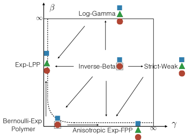
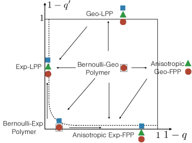
The goal of this paper is twofold. First we obtain the stationary measure of the recently discovered Inverse-Beta polymer. In a few words in the stationary state the free-energy of the DP performs a random walk with Inverse-Beta distributed increments, thus generalizing in a discrete setting the stationary measure of the continuum DP. The existence of this stationary measure is rather natural since the Inverse-Beta polymer is an anisotropic finite temperature model (with two parameters γ,β>0𝛾𝛽0\gamma,\beta>0) of DP on the square lattice which in different limits converges in law to the Log-Gamma (β𝛽\beta\to\infty, the isotropic limit) and Strict-Weak polymer (γ𝛾\gamma\to\infty, the strongly anisotropic limit). These two models possess an exactly known SM that we will generalize to the Inverse-Beta polymer, and our approach will have a strong methodological and conceptual overlap with the one used by Seppäläinen in Seppalainen2012 . Secondly we introduce a new anisotropic 00 temperature model of DP on the square lattice (with two parameters q,q[0,1[q,q^{\prime}\in[0,1[), which we call the Bernoulli-Geometric polymer, and obtain exactly its stationary measure. This model interpolates between the exactly solvable geometric first passage percolation problem studied in OConnell2005 (in the q0𝑞0q\to 0 limit) and the geometric last passage percolation problem e.g. studied in Johansson2000 (in the q0superscript𝑞0q^{\prime}\to 0 limit). The existence of this model was already suggested in usIBeta following the fact that a 00 temperature limit (γ=ϵγ𝛾italic-ϵsuperscript𝛾\gamma=\epsilon\gamma^{\prime} β=ϵβ𝛽italic-ϵsuperscript𝛽\beta=\epsilon\beta^{\prime} and ϵ0italic-ϵ0\epsilon\to 0) of the Inverse-Beta polymer gave an anisotropic generalization of exponential last passage percolation. Since (isotropic) last passage percolation is exactly solvable both for geometric and exponential distribution of random waiting times (the exponential case being the limit q=1γϵ𝑞1superscript𝛾italic-ϵq=1-\gamma^{\prime}\epsilon with ϵ0italic-ϵ0\epsilon\to 0 of the geometric case), it was rather natural to conjecture that an exactly solvable anisotropic generalization of geometric last passage percolation should exist. This motivated the search for such a model. The Bernoulli-Geometric polymer introduced in this paper appears as this missing model, and we thus complement the rich universe of exactly solvable models of DP on the square lattice (see Fig. 1). For the finite temperature case in particular, the only known model not present in this framework is the Beta polymer, which somehow lives in a different class since it has the peculiarity of also being a model of random walk in a random environment BarraquandCorwinBeta ; ThieryLeDoussal2016b .
Refer to caption Refer to caption

Figure 1: The Inverse-Beta polymer is at the center of a large class of finite temperature exactly solvable models of DP on the square lattice with continuous random energies (left), but also admits zero-temperature limiting models (‘below the dashed-line’, in the limit min(γ,β)0min𝛾𝛽0{\rm min(\gamma,\beta)}\to 0). Conversely, the Bernoulli-Geometric polymer introduced in this paper is at the center of a large class of zero-temperature models of DP on the square lattice with discrete random energies (left), but it also admits limiting models with continuous energies (‘below the dashed-line’, in the limit max(q,q)1maxqsuperscriptq1{\rm max(q,q^{\prime})}\to 1), which coincide with the limiting zero-temperature models of the Inverse-Beta polymer. Arrows indicate the possibility of taking a limit from one model to another. The models shown in this picture are defined in Sec. III, Sec. IV.4 and Sec. V.2. Different known exact solvability properties of the various models are here indicated by blue squares for BA solvability, green triangles for RSK or gRSK solvability and by red dots for exactly known stationary measures. The red dots enclosed by a dashed-line (as well as the definition of the Bernoulli-Geometric polymer) are some of the results of this work.

Before we give the main results of the paper and define the Inverse-Beta and Bernoulli-Geometric polymers in Sec. III, let us start by explaining more precisely the general question that is tackled in this article on a simpler model.

II Recall: stationary measure of the Log-Gamma polymer

In this section for pedagogical purposes we recall the stationary measure of the Log-Gamma polymer. The results that we obtain on the stationary measure of the Inverse-Beta polymer can be seen as a generalization of the known results presented in this section to a richer model, and we believe it can be useful for non-specialists to first recall here those simpler results. Specialists on the other hand are encouraged to jump directly to Sec. III.
Refer to caption

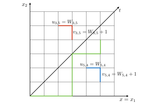
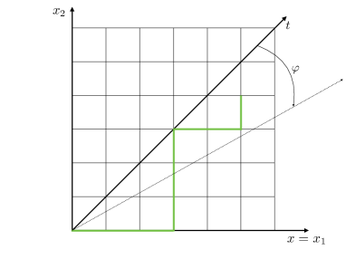
Figure 2: A model of directed polymer on 2superscript2{\mathbb{Z}}^{2}. Green: an admissible (i.e. up/right) polymer path of length t=9𝑡9t=9 with starting point (0,0)00(0,0) and endpoint (x1,x2)=(5,4)subscript𝑥1subscript𝑥254(x_{1},x_{2})=(5,4). We are interested in the stationarity properties that are reached in the limit of long polymers in a given direction φ𝜑\varphi.

Let us first consider the case of an abstract, homogeneous model of directed polymer on the square lattice with on-site disorder: the random environment is defined by drawing random Boltzmann weights Wx1,x2>0subscript𝑊subscript𝑥1subscript𝑥20W_{x_{1},x_{2}}>0 at each point (x1,x2)subscript𝑥1subscript𝑥2(x_{1},x_{2}) of 2superscript2\mathbb{N}^{2}. Boltzmann weights on different lattice sites are supposed to be independent and homogeneously distributed as a positive random variable (RV) W𝑊W with a probability distribution function PW(W)subscript𝑃𝑊𝑊P_{W}(W). The partition sum of DP with starting point (x1,x2)=(0,0)subscript𝑥1subscript𝑥200(x_{1},x_{2})=(0,0) and endpoint (x1,x2)2subscript𝑥1subscript𝑥2superscript2(x_{1},x_{2})\in\mathbb{N}^{2} is defined by

Zx1,x2:=π:(0,0)(x1,x2)(x1,x2)πWx1,x2,assignsubscript𝑍subscript𝑥1subscript𝑥2subscript:𝜋00subscript𝑥1subscript𝑥2subscriptproductsuperscriptsubscript𝑥1superscriptsubscript𝑥2𝜋subscript𝑊superscriptsubscript𝑥1superscriptsubscript𝑥2\displaystyle Z_{x_{1},x_{2}}:=\sum_{\pi:(0,0)\to(x_{1},x_{2})}\prod_{(x_{1}^{\prime},x_{2}^{\prime})\in\pi}W_{x_{1}^{\prime},x_{2}^{\prime}}\ , (II.1)

where the sum π:(0,0)(x1,x2)subscript:𝜋00subscript𝑥1subscript𝑥2\sum_{\pi:(0,0)\to(x_{1},x_{2})} is over all directed paths, also called up-right paths, from (0,0)00(0,0) to (x1,x2)subscript𝑥1subscript𝑥2(x_{1},x_{2}). Those are the paths such that the only jumps allowed are to the right, i.e. as (x1,x2)(x1+1,x2)subscript𝑥1subscript𝑥2subscript𝑥11subscript𝑥2(x_{1},x_{2})\to(x_{1}+1,x_{2}) or upward, i.e. as (x1,x2)(x1,x2+1)subscript𝑥1subscript𝑥2subscript𝑥1subscript𝑥21(x_{1},x_{2})\to(x_{1},x_{2}+1) (see Fig. 2). For a given model of DP, one would like e.g. to characterize the asymptotic properties of Zx1,x2subscript𝑍subscript𝑥1subscript𝑥2Z_{x_{1},x_{2}} in the limit of long polymers t=x1+x2𝑡subscript𝑥1subscript𝑥2t=x_{1}+x_{2}\to\infty. In this paper we focus on the horizontal and vertical ratios of partition sums defined as

Ux1,x2:=Zx1,x2Zx11,x2,Vx1,x2:=Zx1,x2Zx1,x21 .\displaystyle U_{x_{1},x_{2}}:=\frac{Z_{x_{1},x_{2}}}{Z_{x_{1}-1,x_{2}}}\quad,\quad V_{x_{1},x_{2}}:=\frac{Z_{x_{1},x_{2}}}{Z_{x_{1},x_{2}-1}} \ . (II.2)

Introducing the variables t=x1+x2𝑡subscript𝑥1subscript𝑥2t=x_{1}+x_{2} (the length of the polymers) and x=x1𝑥subscript𝑥1x=x_{1} and the notations Ut(x):=Ux,txassignsubscript𝑈𝑡𝑥subscript𝑈𝑥𝑡𝑥U_{t}(x):=U_{x,t-x} and Vt(x):=Vx,txassignsubscript𝑉𝑡𝑥subscript𝑉𝑥𝑡𝑥V_{t}(x):=V_{x,t-x}, we are interested in obtaining the distribution of these RVs in the limit of long polymers in a given direction. That is, for a given φ]1/2,1/2[\varphi\in]-1/2,1/2[ (see Fig. 2) and Tfor-all𝑇superscript\forall T\in{\mathbb{N}}^{*}, X𝑋superscriptX\in{\mathbb{N}}^{*}, we are interested in the set of RVs

(U~t(x),V~t(x))t[0,T],x[X,X]:=limt(Ut+t((1/2+φ)t+x),Vt+t((1/2+φ)t+x))t[0,T],x[X,X].assignsubscriptsubscript~𝑈superscript𝑡superscript𝑥subscript~𝑉superscript𝑡superscript𝑥formulae-sequencesuperscript𝑡0𝑇superscript𝑥𝑋𝑋subscript𝑡subscriptsubscript𝑈𝑡superscript𝑡12𝜑𝑡superscript𝑥subscript𝑉𝑡superscript𝑡12𝜑𝑡superscript𝑥formulae-sequencesuperscript𝑡0𝑇superscript𝑥𝑋𝑋\displaystyle\left(\tilde{U}_{t^{\prime}}(x^{\prime}),\tilde{V}_{t^{\prime}}(x^{\prime})\right)_{t^{\prime}\in[0,T],x^{\prime}\in[-X,X]}:=\lim_{t\to\infty}\left(U_{t+t^{\prime}}((1/2+\varphi)t+x^{\prime}),V_{t+t^{\prime}}((1/2+\varphi)t+x^{\prime})\right)_{t^{\prime}\in[0,T],x^{\prime}\in[-X,X]}\ . (II.3)

The only known finite temperature model of DP on 2superscript2{\mathbb{Z}}^{2} with on-site disorder (i.e. defined as above) for which characterizing exactly the properties of the asymptotic process (U~t(x),V~t(x))t[0,T],x[X,X]subscriptsubscript~𝑈superscript𝑡superscript𝑥subscript~𝑉superscript𝑡superscript𝑥formulae-sequencesuperscript𝑡0𝑇superscript𝑥𝑋𝑋\left(\tilde{U}_{t^{\prime}}(x^{\prime}),\tilde{V}_{t^{\prime}}(x^{\prime})\right)_{t^{\prime}\in[0,T],x^{\prime}\in[-X,X]} is possible is the Log-Gamma polymer. In this case, the random Boltzmann weights are distributed as the inverse of a gamma random variable: WGamma(γ)1similar-to𝑊𝐺𝑎𝑚𝑚𝑎superscript𝛾1W\sim Gamma(\gamma)^{-1}. Here similar-to\sim means ‘distributed as’ and we recall that a RV x𝑥x is gamma distributed with parameter α>0𝛼0\alpha>0 if its PDF is p(x)=1Γ(α)x1+αexθ(x)𝑝𝑥1Γ𝛼superscript𝑥1𝛼superscript𝑒𝑥𝜃𝑥p(x)=\frac{1}{\Gamma(\alpha)}x^{-1+\alpha}e^{-x}\theta(x) (ΓΓ\Gamma is the Euler’s gamma function and θ𝜃\theta is the Heaviside theta function). For this special choice of distribution, although it is not mathematically fully proven, the (mathematically rigorous) results of Seppalainen2012 ; Seppalainen2015 lead to the conjecture that in this case

At fixed t[0,T]superscript𝑡0𝑇t^{\prime}\in[0,T] the variables (U~t(x))x[X,X]subscriptsubscript~𝑈superscript𝑡superscript𝑥superscript𝑥𝑋𝑋(\tilde{U}_{t^{\prime}}(x^{\prime}))_{x^{\prime}\in[-X,X]} and (V~t(x))x[X,X]subscriptsubscript~𝑉superscript𝑡superscript𝑥superscript𝑥𝑋𝑋(\tilde{V}_{t^{\prime}}(x^{\prime}))_{x^{\prime}\in[-X,X]} are all independent and distributed as U~t(x)Gamma(γλ)1similar-tosubscript~𝑈superscript𝑡superscript𝑥𝐺𝑎𝑚𝑚𝑎superscript𝛾𝜆1\tilde{U}_{t^{\prime}}(x^{\prime})\sim Gamma(\gamma-\lambda)^{-1} and V~t(x)Gamma(λ)1similar-tosubscript~𝑉superscript𝑡superscript𝑥𝐺𝑎𝑚𝑚𝑎superscript𝜆1\tilde{V}_{t^{\prime}}(x^{\prime})\sim Gamma(\lambda)^{-1}. The additional parameter λ ]0,γ[\lambda \in]0,\gamma[ depends on φ𝜑\varphi and is the solution of the equation 0=(1/2+φ)ψ(γλ)+(1/2φ)ψ(λ)012𝜑superscript𝜓𝛾𝜆12𝜑superscript𝜓𝜆0=-(1/2+\varphi)\psi^{\prime}(\gamma-\lambda)+(1/2-\varphi)\psi^{\prime}(\lambda), where ψ(x)=Γ(x)/Γ(x)𝜓𝑥superscriptΓ𝑥Γ𝑥\psi(x)=\Gamma^{\prime}(x)/\Gamma(x) is the digamma function.

An additional property of reversibility of the process is known from Seppalainen2012 . These properties rely on a non trivial property of gamma distributions (see Lemma 3.2 in Seppalainen2012 ). Moreover, Lemma 3.2 of Seppalainen2012 also suggests that the Log-Gamma polymer is the only model with on-site disorder for which it is possible to obtain exactly the stationary measure. One of the purposes of this paper is to show that it is also possible to obtain exactly the stationary measure in the Inverse-Beta polymer, an anisotropic finite temperature model of DP on 2superscript2{\mathbb{Z}}^{2} with on-edge disorder that generalizes both the Log-Gamma and Strict-Weak models. We also obtain similar results for the Bernoulli-Geometric polymer, a related zero temperature model that we introduce in this paper.

III Overview: definitions, main results and outline

III.1 Definitions of the models of directed polymers

III.1.1 General notations

All the models of DPs considered in this paper live on the square lattice 2superscript2{\mathbb{Z}}^{2}. We will consider two coordinate systems on 2superscript2{\mathbb{Z}}^{2}, the usual Euclidean coordinates (x1,x2)2subscript𝑥1subscript𝑥2superscript2(x_{1},x_{2})\in{\mathbb{Z}}^{2} and the (t,x)𝑡𝑥(t,x) coordinates t=x1+x2𝑡subscript𝑥1subscript𝑥2t=x_{1}+x_{2} and x=x1𝑥subscript𝑥1x=x_{1} (see Fig.3). The variable t𝑡t will often corresponds to the length of the polymers. To avoid confusion, an arbitrary real function on the lattice, f:(x1,x2)2f(x1,x2):𝑓subscript𝑥1subscript𝑥2superscript2𝑓subscript𝑥1subscript𝑥2f:(x_{1},x_{2})\in{\mathbb{Z}}^{2}\to f(x_{1},x_{2})\in{\mathbb{R}} will be denoted either as fx1,x2:=f(x1,x2)assignsubscript𝑓subscript𝑥1subscript𝑥2𝑓subscript𝑥1subscript𝑥2f_{x_{1},x_{2}}:=f(x_{1},x_{2}), or as ft(x)=f(x1=x,x2=tx)subscript𝑓𝑡𝑥𝑓formulae-sequencesubscript𝑥1𝑥subscript𝑥2𝑡𝑥f_{t}(x)=f(x_{1}=x,x_{2}=t-x). The random environment will live on the edges of 2superscript2{\mathbb{Z}}^{2} and we will generally note by e𝑒e an edge of 2superscript2{\mathbb{Z}}^{2}.

III.1.2 Finite temperature models: The Inverse-Beta polymer(s)

We now define three versions of the Inverse-Beta (IB) polymer. The first is the usual point to point IB polymer introduced in usIBeta . Its partition sum will be noted Zx1,x2subscript𝑍subscript𝑥1subscript𝑥2Z_{x_{1},x_{2}}. The second is the IB polymer with boundaries, a model which possesses a stationarity property and whose definition is original to this work. Its partition sum will be noted Z^x1,x2subscript^𝑍subscript𝑥1subscript𝑥2\hat{Z}_{x_{1},x_{2}}. The third model is the IB polymer with a stationary initial condition, with partition sum Zˇx1,x2subscriptˇ𝑍subscript𝑥1subscript𝑥2\check{Z}_{x_{1},x_{2}}, which also possesses a stationary property and whose definition is original to this work. It is intimately linked with the IB polymer with boundaries and is closer in spirit to the stationary models considered for the continuum DP. The first model will be defined by choosing two parameters (γ,β)+2𝛾𝛽superscriptsubscript2(\gamma,\beta)\in{\mathbb{R}}_{+}^{2} (henceforth referred to as the bulk parameters). The others have one additional parameter λ]0,γ[\lambda\in]0,\gamma[, which will specify one stationary measure among a family of stationary measures at fixed (γ,β)𝛾𝛽(\gamma,\beta) (henceforth referred to as the stationarity or boundary parameter). Throughout this work the use of the hat and check notations will permit to distinguish between quantities associated to each model.

Definition III.1.

The point to point IB polymer We recall here the definition of the point to point IB polymer partition sum as studied using Bethe ansatz in usIBeta . To each vertex (x1,x2)2subscript𝑥1subscript𝑥2superscript2(x_{1},x_{2})\in{\mathbb{Z}}^{2} of the square lattice is associated a random variable Wx1,x2+subscript𝑊subscript𝑥1subscript𝑥2subscriptW_{x_{1},x_{2}}\in\mathbb{R}_{+}. The set of RVs {Wx1,x2,(x1,x2)2}subscript𝑊subscript𝑥1subscript𝑥2subscript𝑥1subscript𝑥2superscript2\{W_{x_{1},x_{2}},(x_{1},x_{2})\in\mathbb{Z}^{2}\} consists of independent, identically distributed (iid) RVs distributed as W1B1similar-to𝑊1𝐵1W\sim\frac{1}{B}-1 where B[0,1]𝐵01B\in[0,1] is a Beta RV of parameters γ𝛾\gamma and β>0𝛽0\beta>0. The PDF P(B)𝑃𝐵P(B) of a Beta random variable is

BBeta(γ,β)P(B)=Γ(γ+β)Γ(γ)Γ(β)Bγ1(1B)β1θ(B)θ(1B),similar-to𝐵𝐵𝑒𝑡𝑎𝛾𝛽𝑃𝐵Γ𝛾𝛽Γ𝛾Γ𝛽superscript𝐵𝛾1superscript1𝐵𝛽1𝜃𝐵𝜃1𝐵\displaystyle B\sim Beta(\gamma,\beta)\Longleftrightarrow P(B)=\frac{\Gamma(\gamma+\beta)}{\Gamma(\gamma)\Gamma(\beta)}B^{\gamma-1}(1-B)^{\beta-1}\theta(B)\theta(1-B)\ , (III.1)

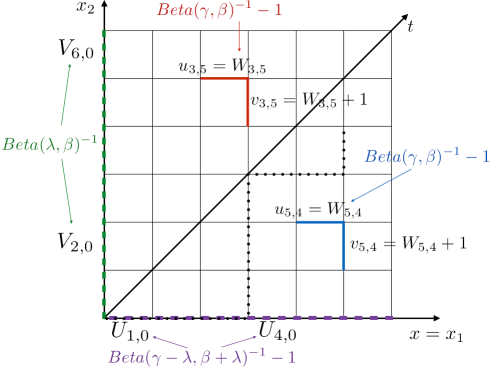
where here and throughout the rest of the paper similar-to\sim means ‘distributed as’, ΓΓ\Gamma is the Euler’s gamma function and θ𝜃\theta is the Heaviside theta function. Given a random environment specified by a drawing of Wx1,x2subscript𝑊subscript𝑥1subscript𝑥2W_{x_{1},x_{2}} at each vertex (x1,x2)2subscript𝑥1subscript𝑥2superscript2(x_{1},x_{2})\in\mathbb{Z}^{2}, we associate to each edge of the square lattice e𝑒e a random Boltzmann weight (BW) w(e)𝑤𝑒w(e) as follows. The random BWs w(e)𝑤𝑒w(e) on horizontal (resp. vertical) edges will be denoted by the letter u𝑢u (resp. v𝑣v) and indexed by the vertex to which they lead (see left of Fig. 3 and beware that we use here the opposite convention compared to usIBeta ), and given in terms of Wx1,x2subscript𝑊subscript𝑥1subscript𝑥2W_{x_{1},x_{2}} by

w((x11,x2)(x1,x2))=ux1,x2=Wx1,x2>0,𝑤subscript𝑥11subscript𝑥2subscript𝑥1subscript𝑥2subscript𝑢subscript𝑥1subscript𝑥2subscript𝑊subscript𝑥1subscript𝑥20\displaystyle w((x_{1}-1,x_{2})\to(x_{1},x_{2}))=u_{x_{1},x_{2}}=W_{x_{1},x_{2}}>0\ ,
w((x11,x2)(x1,x2))=vx1,x2=Wx1,x2+1>1.𝑤subscript𝑥11subscript𝑥2subscript𝑥1subscript𝑥2subscript𝑣subscript𝑥1subscript𝑥2subscript𝑊subscript𝑥1subscript𝑥211\displaystyle w((x_{1}-1,x_{2})\to(x_{1},x_{2}))=v_{x_{1},x_{2}}=W_{x_{1},x_{2}}+1>1\ . (III.2)

Refer to caption , Refer to caption

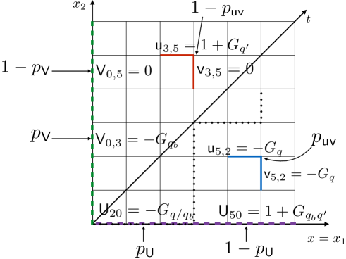
Figure 3: Left: The point to point Inverse-Beta polymer. Blue (resp. Red) : couple of correlated Boltzmann weights on edges arriving at (x1,x2)=(5,4)subscript𝑥1subscript𝑥254(x_{1},x_{2})=(5,4) (resp. (x1,x2)=(3,4)subscript𝑥1subscript𝑥234(x_{1},x_{2})=(3,4)). Green: an admissible (i.e. up/right) polymer path of length t=9𝑡9t=9 with starting point (0,0)00(0,0) and endpoint (x1,x2)=(5,4)subscript𝑥1subscript𝑥254(x_{1},x_{2})=(5,4). Right: The Inverse-Beta polymer with boundaries. The Boltzmann weights in the bulk (blue and red) are the same as in the model without boundaries and are distributed as in (III.3). The random Boltzmann weights on the vertical (dashed-green) and horizontal (dashed-purple) boundaries are distributed as in (III.2). The dotted line represents a possible polymer path from (x1,x2)=(0,0)subscript𝑥1subscript𝑥200(x_{1},x_{2})=(0,0) to (x1,x2)=(5,4)subscript𝑥1subscript𝑥254(x_{1},x_{2})=(5,4).

Hence in this model the BWs on different edges are correlated if and only if they lead to the same vertex, since in this case v=u+1𝑣𝑢1v=u+1, and the vertical direction is always favored compared to the horizontal one. The model is thus anisotropic. It interpolates between two other known exactly solvable models of DP on 2superscript2{\mathbb{Z}}^{2}: the Log-Gamma polymer (isotropic β𝛽\beta\to\infty limit) and the Strict-Weak polymer (γ𝛾\gamma\to\infty limit, see Sec. IV.4). Let us write here for clarity the PDF of W𝑊W, noted PW(W)subscript𝑃𝑊𝑊P_{W}(W):

W1Beta(γ,β)1>0,PW(W)=Γ(γ+β)Γ(γ)Γ(β)(11W+1)β1(1W+1)γ+1θ(W).\displaystyle W\sim\frac{1}{Beta(\gamma,\beta)}-1>0\ \quad,\quad P_{W}(W)=\frac{\Gamma(\gamma+\beta)}{\Gamma(\gamma)\Gamma(\beta)}\left(1-\frac{1}{W+1}\right)^{\beta-1}\left(\frac{1}{W+1}\right)^{\gamma+1}\theta(W). (III.3)

Given a random environment, the partition sum of the point-to-point IB polymer with starting point (0,0)00(0,0) and endpoint (x10,x20)formulae-sequencesubscript𝑥10subscript𝑥20(x_{1}\geq 0,x_{2}\geq 0) is defined as

Zx1,x2=π:(0,0)(x1,x2)eπw(e),subscript𝑍subscript𝑥1subscript𝑥2subscript:𝜋00subscript𝑥1subscript𝑥2subscriptproduct𝑒𝜋𝑤𝑒\displaystyle Z_{x_{1},x_{2}}=\sum_{\pi:(0,0)\to(x_{1},x_{2})}\prod_{e\in\pi}w(e)\ , (III.4)

where here and throughout the rest of this work the sum π:(0,0)(x1,x2)subscript:𝜋00subscript𝑥1subscript𝑥2\sum_{\pi:(0,0)\to(x_{1},x_{2})} is over all directed paths, also called up-right paths, from (0,0)00(0,0) to (x1,x2)subscript𝑥1subscript𝑥2(x_{1},x_{2}). Those are the paths such that the only jumps allowed are either to the right, i.e. as (x1,x2)(x1+1,x2)subscript𝑥1subscript𝑥2subscript𝑥11subscript𝑥2(x_{1},x_{2})\to(x_{1}+1,x_{2}), or upward, i.e. as (x1,x2)(x1,x2+1)subscript𝑥1subscript𝑥2subscript𝑥1subscript𝑥21(x_{1},x_{2})\to(x_{1},x_{2}+1) (see Fig. 3). Equivalently, using the (t,x)𝑡𝑥(t,x) coordinate system the partition sum Zt(x)=Zx,txsubscript𝑍𝑡𝑥subscript𝑍𝑥𝑡𝑥Z_{t}(x)=Z_{x,t-x} is defined recursively as, for t0𝑡0t\geq 0,

Zt(x)=ut(x)Zt1(x1)+vt(x)Zt1(x) for t1formulae-sequencesubscript𝑍𝑡𝑥subscript𝑢𝑡𝑥subscript𝑍𝑡1𝑥1subscript𝑣𝑡𝑥subscript𝑍𝑡1𝑥 for 𝑡1\displaystyle Z_{t}(x)=u_{t}(x)Z_{t-1}(x-1)+v_{t}(x)Z_{t-1}(x)\quad\text{ for }t\geq 1
Zt=0(x)=δx,0,subscript𝑍𝑡0𝑥subscript𝛿𝑥0\displaystyle Z_{t=0}(x)=\delta_{x,0}\ , (III.5)

where δi,jsubscript𝛿𝑖𝑗\delta_{i,j} is the Kronecker delta symbol. Following (III.1), the length of the polymers t𝑡t will also be thought of as a time-like variable, (III.1) being then thought of as a Markov process. The latter is a discrete version of the stochastic-heat-equation satisfied by the partition sum of the continuum DP.

Definition III.2.

The IB polymer with boundaries We define a second version of the IB polymer by changing the BWs on the boundaries of 2superscript2\mathbb{N}^{2}. The random BWs are now denoted by w^(e)^𝑤𝑒\hat{w}(e) and given by

w^((x11,x2)(x1,x2))=ux1,x2=Wx1,x2>0, if x21,\displaystyle\hat{w}((x_{1}-1,x_{2})\to(x_{1},x_{2}))=u_{x_{1},x_{2}}=W_{x_{1},x_{2}}>0\quad,\quad\text{ if }x_{2}\geq 1\ ,
w^((x1,x21)(x1,x2))=vx1,x2=Wx1,x2+1>1, if x11,\displaystyle\hat{w}((x_{1},x_{2}-1)\to(x_{1},x_{2}))=v_{x_{1},x_{2}}=W_{x_{1},x_{2}}+1>1\quad,\quad\text{ if }x_{1}\geq 1\ ,
w^((x11,0)(x1,0))=Ux1,0,^𝑤subscript𝑥110subscript𝑥10subscript𝑈subscript𝑥10\displaystyle\hat{w}((x_{1}-1,0)\to(x_{1},0))=U_{x_{1},0}\ ,
w^((0,x21)(0,x2))=V0,x2.^𝑤0subscript𝑥210subscript𝑥2subscript𝑉0subscript𝑥2\displaystyle\hat{w}((0,x_{2}-1)\to(0,x_{2}))=V_{0,x_{2}}\ . (III.6)

Here the random BWs in the bulk ux1,x2=Wx1,x2subscript𝑢subscript𝑥1subscript𝑥2subscript𝑊subscript𝑥1subscript𝑥2u_{x_{1},x_{2}}=W_{x_{1},x_{2}} and vx1,x2=Wx1,x2+1subscript𝑣subscript𝑥1subscript𝑥2subscript𝑊subscript𝑥1subscript𝑥21v_{x_{1},x_{2}}=W_{x_{1},x_{2}}+1 for x1,x21subscript𝑥1subscript𝑥21x_{1},x_{2}\geq 1 are distributed as before (see (III.1)), and the BWs on the boundaries are all independent and distributed as Ux1,0Usimilar-tosubscript𝑈subscript𝑥10𝑈U_{x_{1},0}\sim U and V0,x2Vsimilar-tosubscript𝑉0subscript𝑥2𝑉V_{0,x_{2}}\sim V where

U1Beta(γλ,β+λ)1>0,PU(U)=Γ(γ+β)Γ(γλ)Γ(β+λ)(11U+1)β+λ1(1U+1)γλ+1θ(U),\displaystyle U\sim\frac{1}{Beta(\gamma-\lambda,\beta+\lambda)}-1>0\quad,\quad P_{U}(U)=\frac{\Gamma(\gamma+\beta)}{\Gamma(\gamma-\lambda)\Gamma(\beta+\lambda)}\left(1-\frac{1}{U+1}\right)^{\beta+\lambda-1}\left(\frac{1}{U+1}\right)^{\gamma-\lambda+1}\theta(U),
V1Beta(λ,β)>1,PV(V)=Γ(λ+β)Γ(λ)Γ(β)(11V)β1(1V)λ+1θ(V1).\displaystyle V\sim\frac{1}{Beta(\lambda,\beta)}>1\quad,\quad P_{V}(V)=\frac{\Gamma(\lambda+\beta)}{\Gamma(\lambda)\Gamma(\beta)}\left(1-\frac{1}{V}\right)^{\beta-1}\left(\frac{1}{V}\right)^{\lambda+1}\theta(V-1)\ . (III.7)

Here 0<λ<γ0𝜆𝛾0<\lambda<\gamma is an additional parameter and we have written explicitly the PDF PU(U)subscript𝑃𝑈𝑈P_{U}(U) and PV(V)subscript𝑃𝑉𝑉P_{V}(V) of U𝑈U and V𝑉V that easily follow from (III.1). In the following we will refer to λ𝜆\lambda as the boundary or stationarity parameter. We consider again the partition sum for polymers with starting point (0,0)00(0,0) and endpoint (x10,x20)formulae-sequencesubscript𝑥10subscript𝑥20(x_{1}\geq 0,x_{2}\geq 0), defined as

Z^x1,x2=π:(0,0)(x1,x2)eπw^(e).subscript^𝑍subscript𝑥1subscript𝑥2subscript:𝜋00subscript𝑥1subscript𝑥2subscriptproduct𝑒𝜋^𝑤𝑒\displaystyle\hat{Z}_{x_{1},x_{2}}=\sum_{\pi:(0,0)\to(x_{1},x_{2})}\prod_{e\in\pi}\hat{w}(e)\ . (III.8)
Definition III.3.

The IB polymer with stationary initial condition We define a third version of the IB polymer. Following the recursion equation (III.1), we define the DP partition sum Zˇt(x)subscriptˇ𝑍𝑡𝑥\check{Z}_{t}(x) for t1𝑡1t\geq-1 and x𝑥x\in{\mathbb{Z}} as

Zˇt(x)=ut(x)Zˇt1(x1)+vt(x)Zˇt1(x) for t1formulae-sequencesubscriptˇ𝑍𝑡𝑥subscript𝑢𝑡𝑥subscriptˇ𝑍𝑡1𝑥1subscript𝑣𝑡𝑥subscriptˇ𝑍𝑡1𝑥 for 𝑡1\displaystyle\check{Z}_{t}(x)=u_{t}(x)\check{Z}_{t-1}(x-1)+v_{t}(x)\check{Z}_{t-1}(x)\quad\text{ for }t\geq 1 (III.9)

and with the initial condition

Zˇ0(0)=1,Zˇ0(x)Zˇ1(x1)=U(x),Zˇ0(x)Zˇ1(x)=V(x) for x.\displaystyle\check{Z}_{0}(0)=1\quad,\quad\frac{\check{Z}_{0}(x)}{\check{Z}_{-1}(x-1)}=U(x)\quad,\quad\frac{\check{Z}_{0}(x)}{\check{Z}_{-1}(x)}=V(x)\quad\text{ for }x\in{\mathbb{Z}}\ . (III.10)

Where (U(x))xsubscript𝑈𝑥𝑥(U(x))_{x\in{\mathbb{Z}}} and (V(x))xsubscript𝑉𝑥𝑥(V(x))_{x\in{\mathbb{Z}}} are two sets of iid RVs distributed as U(x)Usimilar-to𝑈𝑥𝑈U(x)\sim U and V(x)Vsimilar-to𝑉𝑥𝑉V(x)\sim V with U,V𝑈𝑉U,V distributed as (III.2), while the RVs (ut(x),vt(x))subscript𝑢𝑡𝑥subscript𝑣𝑡𝑥(u_{t}(x),v_{t}(x)) are distributed as before (III.1). The definition of Zt(x)subscript𝑍𝑡𝑥Z_{t}(x) for t=1𝑡1t=-1 is for future notational convenience and for what concerns Zt(x)subscript𝑍𝑡𝑥Z_{t}(x) for t0𝑡0t\geq 0 it is equivalent to set the initial condition as Zˇ0(x+1)/Zˇ0(x)=U(x+1)/V(x)subscriptˇ𝑍0𝑥1subscriptˇ𝑍0𝑥𝑈𝑥1𝑉𝑥\check{Z}_{0}(x+1)/\check{Z}_{0}(x)=U(x+1)/V(x). This model is analogous to the point to Brownian continuum DP.

III.1.3 Zero temperature models: The Bernoulli-Geometric polymer(s)

We now define as previously for the Inverse-Beta polymer three versions of the Bernoulli-Geometric (BG) polymer: the point to point BG polymer, the BG polymer with boundaries and the BG polymer with stationary initial condition. The first model will be defined by choosing two (‘bulk’) parameters (q,q)[0,1[2(q,q^{\prime})\in[0,1[^{2}. The others have one additional (‘boundary’ or ‘stationarity’) parameter qb]q,1[q_{b}\in]q,1[, which will specify one stationary measure among a family of stationary measures at fixed (q,q)𝑞superscript𝑞(q,q^{\prime}). All definitions of this section are to our knowledge original to this work. Here and throughout the paper the similarities between these models and the IB polymers will be highlighted using similar notations, with the convention that we reserve sans-serif letters for the BG polymers. The connection between the IB and BG polymers, which was the main motivation for introducing the BG polymer, was already mentioned in the introduction. It will be made more precise in Sec. V.2.

Definition III.4.

The point to point Bernoulli-Geometric polymer We now define the Bernoulli-Geometric polymer. We assign to each edge e𝑒e of 2superscript2{\mathbb{Z}}^{2} a discrete random energy (e)𝑒{\cal E}(e)\in{\mathbb{Z}}. Depending on whether the edge is horizontal or vertical, the random energies are drawn from different probability distributions. Let us introduce the notation

((x1,x2)(x1+1,x2))=𝗎x1+1,x2,subscript𝑥1subscript𝑥2subscript𝑥11subscript𝑥2subscript𝗎subscript𝑥11subscript𝑥2\displaystyle{\cal E}\left((x_{1},x_{2})\to(x_{1}+1,x_{2})\right)={\sf u}_{x_{1}+1,x_{2}}\ ,
((x1,x2)(x1,x2+1))=𝗏x1,x2+1,subscript𝑥1subscript𝑥2subscript𝑥1subscript𝑥21subscript𝗏subscript𝑥1subscript𝑥21\displaystyle{\cal E}\left((x_{1},x_{2})\to(x_{1},x_{2}+1)\right)={\sf v}_{x_{1},x_{2}+1}\ , (III.11)

hence 𝗎𝗎{\sf u} (resp. 𝗏𝗏{\sf v}) denotes a random energy on an horizontal (resp. vertical) edge. We suppose that couples of random variables indexed by the endpoint of the edges (𝗎x1,x2,𝗏x1,x2)subscript𝗎subscript𝑥1subscript𝑥2subscript𝗏subscript𝑥1subscript𝑥2({\sf u}_{x_{1},x_{2}},{\sf v}_{x_{1},x_{2}}) are iid RVs distributed as (𝗎x1,x2,𝗏x1,x2)(𝗎,𝗏)similar-tosubscript𝗎subscript𝑥1subscript𝑥2subscript𝗏subscript𝑥1subscript𝑥2𝗎𝗏({\sf u}_{x_{1},x_{2}},{\sf v}_{x_{1},x_{2}})\sim({\sf u},{\sf v}) where the couple (𝗎,𝗏)𝗎𝗏({\sf u},{\sf v}) is distributed as

𝗎(1ζ𝗎𝗏)(1+Gq)ζ𝗎𝗏Gq,similar-to𝗎1subscript𝜁𝗎𝗏1subscript𝐺superscript𝑞subscript𝜁𝗎𝗏subscript𝐺𝑞\displaystyle{\sf u}\sim(1-\zeta_{{\sf u}{\sf v}})(1+G_{q^{\prime}})-\zeta_{{\sf u}{\sf v}}G_{q}\in{\mathbb{Z}}\ ,
𝗏ζ𝗎𝗏Gq,similar-to𝗏subscript𝜁𝗎𝗏subscript𝐺𝑞subscript\displaystyle{\sf v}\sim-\zeta_{{\sf u}{\sf v}}G_{q}\in{\mathbb{Z}}_{-}\ , (III.12)

where 0<q<10𝑞10<q<1 and 0<q<10superscript𝑞10<q^{\prime}<1 are the two parameters of the models and Gqsubscript𝐺𝑞G_{q}, Gqsubscript𝐺superscript𝑞G_{q^{\prime}} and ζ𝗎𝗏subscript𝜁𝗎𝗏\zeta_{{\sf u}{\sf v}} are independent RVs distributed as follows. Gqsubscript𝐺𝑞G_{q}\in{\mathbb{N}} and Gqsubscript𝐺superscript𝑞G_{q^{\prime}}\in{\mathbb{N}} are geometric RVs with parameters q𝑞q and qsuperscript𝑞q^{\prime} with the convention

Proba(Gq=k)=(1q)qk,𝑃𝑟𝑜𝑏𝑎subscript𝐺𝑞𝑘1𝑞superscript𝑞𝑘\displaystyle Proba(G_{q}=k\in{\mathbb{N}})=(1-q)q^{k}\ , (III.13)

and similarly for Gqsubscript𝐺superscript𝑞G_{q^{\prime}} with the exchange qq𝑞superscript𝑞q\to q^{\prime}. ζ𝗎𝗏{0,1}subscript𝜁𝗎𝗏01\zeta_{{\sf u}{\sf v}}\in\{0,1\} is a Bernoulli RV with parameter p𝗎𝗏subscript𝑝𝗎𝗏p_{{\sf u}{\sf v}} given by

p𝗎𝗏=1q1qq]0,1[,\displaystyle p_{{\sf u}{\sf v}}=\frac{1-q^{\prime}}{1-qq^{\prime}}\in]0,1[\ , (III.14)

and thus

Proba(ζ𝗎𝗏=1)=p𝗎𝗏,Proba(ζ𝗎𝗏=0)=1p𝗎𝗏.\displaystyle Proba(\zeta_{{\sf u}{\sf v}}=1)=p_{{\sf u}{\sf v}}\quad,\quad Proba(\zeta_{{\sf u}{\sf v}}=0)=1-p_{{\sf u}{\sf v}}\ . (III.15)

As such, 𝗎𝗏𝗎𝗏{\sf u}\geq{\sf v} (equality occurring whenever ζ𝗎𝗏=1subscript𝜁𝗎𝗏1\zeta_{{\sf u}{\sf v}}=1) and note that 𝗎𝗎{\sf u}\in{\mathbb{Z}} can be positive or negative while 𝗏𝗏subscript{\sf v}\in{\mathbb{Z}}_{-} is always negative (or zero). 𝗎𝗎{\sf u} and 𝗏𝗏{\sf v} are correlated RVs since they are both functions of the same Bernoulli RV ζ𝗎𝗏subscript𝜁𝗎𝗏\zeta_{{\sf u}{\sf v}}. Note that one can also add correlations between Gqsubscript𝐺𝑞G_{q} and Gqsubscript𝐺superscript𝑞G_{q^{\prime}}: since ζ𝗎𝗏{0,1}subscript𝜁𝗎𝗏01\zeta_{{\sf u}{\sf v}}\in\{0,1\} one easily shows that correlations between Gqsubscript𝐺𝑞G_{q} and Gqsubscript𝐺superscript𝑞G_{q^{\prime}} do not affect the PDF of (𝗎,𝗏)𝗎𝗏({\sf u},{\sf v}). The latter can be written as

Proba(𝗎=k𝗎,𝗏=k𝗏)=\displaystyle Proba({\sf u}=k_{{\sf u}}\in{\mathbb{Z}},{\sf v}=k_{{\sf v}}\in{\mathbb{Z}}_{-})= p𝗎𝗏δ(k𝗎=k𝗏)δ(k𝗏0)(1q)qk𝗏subscript𝑝𝗎𝗏𝛿subscript𝑘𝗎subscript𝑘𝗏𝛿subscript𝑘𝗏01𝑞superscript𝑞subscript𝑘𝗏\displaystyle p_{{\sf u}{\sf v}}\delta(k_{{\sf u}}=k_{{\sf v}})\delta(k_{{\sf v}}\leq 0)(1-q)q^{-k_{{\sf v}}} (III.16)
+(1p𝗎𝗏)δ(k𝗏=0)δ(k𝗎1)(1q)(q)k𝗎1,1subscript𝑝𝗎𝗏𝛿subscript𝑘𝗏0𝛿subscript𝑘𝗎11superscript𝑞superscriptsuperscript𝑞subscript𝑘𝗎1\displaystyle+(1-p_{{\sf u}{\sf v}})\delta(k_{{\sf v}}=0)\delta(k_{{\sf u}}\geq 1)(1-q^{\prime})(q^{\prime})^{k_{{\sf u}}-1}\ ,

where here and throughout the rest of the paper the symbol δ𝛿\delta is used to denote the indicator function of the set specified inside the δ𝛿\delta. Finally, given a random environment specified by a drawing of the random energies (𝗎x1,x2,𝗏x1,x2)subscript𝗎subscript𝑥1subscript𝑥2subscript𝗏subscript𝑥1subscript𝑥2({\sf u}_{x_{1},x_{2}},{\sf v}_{x_{1},x_{2}}), we are interested in the optimal energy to go from the origin (0,0)00(0,0) to the point (x1,x2)subscript𝑥1subscript𝑥2(x_{1},x_{2})

𝖤x1,x2=min{(π)=eπ(e),π:(0,0)(x1,x2)}.subscript𝖤subscript𝑥1subscript𝑥2𝜋subscript𝑒𝜋𝑒:𝜋00subscript𝑥1subscript𝑥2\displaystyle{\sf E}_{x_{1},x_{2}}={\rm\min}\left\{{\cal E}(\pi)=\sum_{e\in\pi}{\cal E}(e),\pi:(0,0)\to(x_{1},x_{2})\right\}\ . (III.17)

Where as before the minimization is over up-right paths. Assigning for convention the value 𝖤x1,x2=+subscript𝖤subscript𝑥1subscript𝑥2{\sf E}_{x_{1},x_{2}}=+\infty for vertices (x1,x2)subscript𝑥1subscript𝑥2(x_{1},x_{2}) with either x1<0subscript𝑥10x_{1}<0 or x2<0subscript𝑥20x_{2}<0, the model can also be recursively defined as, using the (t,x)𝑡𝑥(t,x) coordinates

𝖤t(x)=min(𝖤t1(x1)+𝗎t(x),𝖤t1(x)+𝗏t(x)) for t1,subscript𝖤𝑡𝑥subscript𝖤𝑡1𝑥1subscript𝗎𝑡𝑥subscript𝖤𝑡1𝑥subscript𝗏𝑡𝑥 for 𝑡1\displaystyle{\sf E}_{t}(x)={\rm\min}\left({\sf E}_{t-1}(x-1)+{\sf u}_{t}(x),{\sf E}_{t-1}(x)+{\sf v}_{t}(x)\right)\text{ for }t\geq 1\ ,
𝖤t=0(0)=0and𝖤t=0(x)=+forx0.formulae-sequencesubscript𝖤𝑡000andformulae-sequencesubscript𝖤𝑡0𝑥for𝑥0\displaystyle{\sf E}_{t=0}(0)=0\quad\text{and}\quad{\sf E}_{t=0}(x)=+\infty\quad\text{for}\quad x\neq 0\ . (III.18)

The definition of this model is, to our knowledge, original to this work. The model can be defined for any value of the parameter p𝗎𝗏[0,1]subscript𝑝𝗎𝗏01p_{{\sf u}{\sf v}}\in[0,1], but it is only for the value given by (III.14) that we can write down exactly its stationary measure. This precise value thus makes the model special, in the sense that it possesses an ESP. In this model the parameters q𝑞q and qsuperscript𝑞q^{\prime} do not play symmetric roles: qsuperscript𝑞q^{\prime} can be thought of as an anisotropy parameter which favors the vertical edges by sometimes (with probability 1p𝗎𝗏=q1q1qq1subscript𝑝𝗎𝗏superscript𝑞1𝑞1𝑞superscript𝑞1-p_{{\sf u}{\sf v}}=q^{\prime}\frac{1-q}{1-qq^{\prime}}) putting a penalty on horizontal edges. Two important limits are an isotropic limit of the model which is obtained by setting q0superscript𝑞0q^{\prime}\to 0, and an anisotropic limit which is obtained for q0𝑞0q\to 0. In the isotropic limit p𝗎𝗏=1subscript𝑝𝗎𝗏1p_{{\sf u}{\sf v}}=1 and the model corresponds to a problem of last passage percolation, while in the anisotropic limit p𝗎𝗏=0subscript𝑝𝗎𝗏0p_{{\sf u}{\sf v}}=0 and the model corresponds to a problem of first passage percolation (see Sec. V.2). More generally the Bernoulli-Geometric polymer thus mixes an optimization problem of the first-passage type with an optimization problem of the last-passage type. In this interpretation p𝗎𝗏subscript𝑝𝗎𝗏p_{{\sf u}{\sf v}} is a mixing parameter which must have the precise value (III.14) for the model to be exactly solvable. Interesting continuous limits are also obtained by letting q,q1𝑞superscript𝑞1q,q^{\prime}\to 1. There the model converges to the zero temperature limit of the Inverse-Beta polymer. This will be further discussed in Sec. V.2.
Refer to caption

Figure 4: The Bernoulli-Geometric polymer with boundaries. In the bulk the couple of energies on the edges (𝗎,𝗏)𝗎𝗏({\sf u},{\sf v}) are taken with probability p𝗎𝗏subscript𝑝𝗎𝗏p_{{\sf u}{\sf v}} (resp. (1p𝗎𝗏)1subscript𝑝𝗎𝗏(1-p_{{\sf u}{\sf v}})) as (𝗎,𝗏)=(Gq,Gq)𝗎𝗏subscript𝐺𝑞subscript𝐺𝑞({\sf u},{\sf v})=(-G_{q},-G_{q}) (blue edges above) (resp. (𝗎,𝗏)=(1+Gq,0)𝗎𝗏1subscript𝐺superscript𝑞0({\sf u},{\sf v})=(1+G_{q^{\prime}},0) (red edges above)). The energies on the horizontal boundary 𝖴𝖴{\sf U} (dashed-purple) are taken with probability p𝖴subscript𝑝𝖴p_{{\sf U}} (resp. 1p𝖴1subscript𝑝𝖴1-p_{{\sf U}}) as 𝖴=Gq/qb𝖴subscript𝐺𝑞subscript𝑞𝑏{\sf U}=-G_{q/q_{b}} (resp. 𝖴=1+Gqbq𝖴1subscript𝐺subscript𝑞𝑏superscript𝑞{\sf U}=1+G_{q_{b}q^{\prime}}). The energies on the vertical boundary 𝖵𝖵{\sf V} (dashed-green) are taken with probability p𝖵subscript𝑝𝖵p_{{\sf V}} (resp. 1p𝖵1subscript𝑝𝖵1-p_{{\sf V}}) as 𝖵=Gqb𝖵subscript𝐺subscript𝑞𝑏{\sf V}=-G_{q_{b}} (resp. 𝖴=1+Gqbq𝖴1subscript𝐺subscript𝑞𝑏superscript𝑞{\sf U}=1+G_{q_{b}q^{\prime}}). The dotted line represents a possible polymer path from (x1,x2)=(0,0)subscript𝑥1subscript𝑥200(x_{1},x_{2})=(0,0) to (x1,x2)=(5,4)subscript𝑥1subscript𝑥254(x_{1},x_{2})=(5,4).
Definition III.5.

The BG polymer with boundaries We now consider the BG model previously defined and change the distribution of energies on the boundaries of 2superscript2\mathbb{N}^{2}. In the model with boundaries the energy on the edges ^(e)^𝑒\hat{\cal E}(e) are distributed as

^((x1,x2)(x1+1,x2))=𝗎x1+1,x2 if x21,^subscript𝑥1subscript𝑥2subscript𝑥11subscript𝑥2subscript𝗎subscript𝑥11subscript𝑥2 if subscript𝑥21\displaystyle\hat{\cal E}\left((x_{1},x_{2})\to(x_{1}+1,x_{2})\right)={\sf u}_{x_{1}+1,x_{2}}\text{ if }x_{2}\geq 1,
^((x1,x2)(x1,x2+1))=𝗏x1,x2+1 if x11,^subscript𝑥1subscript𝑥2subscript𝑥1subscript𝑥21subscript𝗏subscript𝑥1subscript𝑥21 if subscript𝑥11\displaystyle\hat{\cal E}\left((x_{1},x_{2})\to(x_{1},x_{2}+1)\right)={\sf v}_{x_{1},x_{2}+1}\text{ if }x_{1}\geq 1\ ,
^((x1,0)(x1+1,0))=𝖴x1+1,0,^subscript𝑥10subscript𝑥110subscript𝖴subscript𝑥110\displaystyle\hat{\cal E}\left((x_{1},0)\to(x_{1}+1,0)\right)={\sf U}_{x_{1}+1,0}\ ,
^((0,x2)(0,x2+1))=𝖵0,x2+1.^0subscript𝑥20subscript𝑥21subscript𝖵0subscript𝑥21\displaystyle\hat{\cal E}\left((0,x_{2})\to(0,x_{2}+1)\right)={\sf V}_{0,x_{2}+1}\ . (III.19)

Where here the random energies in the bulk (𝗎x1,x2,𝗏x1,x2)|x1,x21(𝗎,𝗏)similar-toevaluated-atsubscript𝗎subscript𝑥1subscript𝑥2subscript𝗏subscript𝑥1subscript𝑥2subscript𝑥1subscript𝑥21𝗎𝗏({\sf u}_{x_{1},x_{2}},{\sf v}_{x_{1},x_{2}})|_{x_{1},x_{2}\geq 1}\sim({\sf u},{\sf v}) are distributed as before with parameters 0<q<10𝑞10<q<1 and 0<q<10superscript𝑞10<q^{\prime}<1, see (III.4) and (III.16). The random energies on the edges of 2superscript2{\mathbb{N}}^{2}, 𝖴x11,0subscript𝖴subscript𝑥110{\sf U}_{x_{1}\geq 1,0} and 𝖵0,x21subscript𝖵0subscript𝑥21{\sf V}_{0,x_{2}\geq 1} are independent from the random energies in the bulk and from each other. They are distributed as 𝖴x1,0𝖴similar-tosubscript𝖴subscript𝑥10𝖴{\sf U}_{x_{1},0}\sim{\sf U} and 𝖵0,x2𝖵similar-tosubscript𝖵0subscript𝑥2𝖵{\sf V}_{0,x_{2}}\sim{\sf V} where

𝖴(1ζ𝖴)(1+Gqbq)ζ𝖴Gq/qb,similar-to𝖴1subscript𝜁𝖴1subscript𝐺subscript𝑞𝑏superscript𝑞subscript𝜁𝖴subscript𝐺𝑞subscript𝑞𝑏\displaystyle{\sf U}\sim(1-\zeta_{{\sf U}})(1+G_{q_{b}q^{\prime}})-\zeta_{{\sf U}}G_{q/q_{b}}\in{\mathbb{Z}}\ ,
𝖵ζ𝖵Gqb.similar-to𝖵subscript𝜁𝖵subscript𝐺subscript𝑞𝑏subscript\displaystyle{\sf V}\sim-\zeta_{{\sf V}}G_{q_{b}}\in{\mathbb{Z}}_{-}\ . (III.20)

Here q<qb<1𝑞subscript𝑞𝑏1q<q_{b}<1 is a new parameter, Gqbsubscript𝐺subscript𝑞𝑏G_{q_{b}}, Gq/qbsubscript𝐺𝑞subscript𝑞𝑏G_{q/q_{b}} and Gqbqsubscript𝐺subscript𝑞𝑏superscript𝑞G_{q_{b}q^{\prime}} are independent geometric RVs distributed as in (III.13), while ζ𝖴subscript𝜁𝖴\zeta_{{\sf U}} and ζ𝖵subscript𝜁𝖵\zeta_{{\sf V}} are Bernoulli RVs with parameter p𝖴subscript𝑝𝖴p_{{\sf U}} and p𝖵subscript𝑝𝖵p_{{\sf V}} distributed as in (III.15) with

p𝖴=1qbq1qq,p𝖵=1q1qbq.\displaystyle p_{{\sf U}}=\frac{1-q_{b}q^{\prime}}{1-qq^{\prime}}\quad,\quad p_{{\sf V}}=\frac{1-q^{\prime}}{1-q_{b}q^{\prime}}\ . (III.21)

We can also directly write the probability distribution of 𝖴𝖴{\sf U} and 𝖵𝖵{\sf V} as

Proba(𝖴=k𝖴)=𝑃𝑟𝑜𝑏𝑎𝖴subscript𝑘𝖴absent\displaystyle Proba({\sf U}=k_{{\sf U}}\in{\mathbb{Z}})= p𝖴δ(k𝖴0)(1q/qb)(q/qb)k𝖴subscript𝑝𝖴𝛿subscript𝑘𝖴01𝑞subscript𝑞𝑏superscript𝑞subscript𝑞𝑏subscript𝑘𝖴\displaystyle p_{{\sf U}}\delta(k_{{\sf U}}\leq 0)(1-q/q_{b})(q/q_{b})^{-k_{{\sf U}}}
+(1p𝖴)δ(k𝖴1)(1qbq)(qbq)k𝖴1,1subscript𝑝𝖴𝛿subscript𝑘𝖴11subscript𝑞𝑏superscript𝑞superscriptsubscript𝑞𝑏superscript𝑞subscript𝑘𝖴1\displaystyle+(1-p_{{\sf U}})\delta(k_{{\sf U}}\geq 1)(1-q_{b}q^{\prime})(q_{b}q^{\prime})^{k_{{\sf U}}-1}\ ,
Proba(𝖵=k𝖵)=𝑃𝑟𝑜𝑏𝑎𝖵subscript𝑘𝖵subscriptabsent\displaystyle Proba({\sf V}=k_{{\sf V}}\in{\mathbb{Z}}_{-})= p𝖵δ(k𝖵0)(1qb)(qb)k𝖵+(1p𝖵)δ(k𝖵=0).subscript𝑝𝖵𝛿subscript𝑘𝖵01subscript𝑞𝑏superscriptsubscript𝑞𝑏subscript𝑘𝖵1subscript𝑝𝖵𝛿subscript𝑘𝖵0\displaystyle p_{{\sf V}}\delta(k_{{\sf V}}\leq 0)(1-q_{b})(q_{b})^{-k_{{\sf V}}}+(1-p_{{\sf V}})\delta(k_{{\sf V}}=0)\ . (III.22)

Given a random environment specified by a drawing of the bulk and edges random energies we are interested in the optimal energy to go from the origin (0,0)00(0,0) to the point (x1,x2)subscript𝑥1subscript𝑥2(x_{1},x_{2})

𝖤^x1,x2=min{^(π)=eπ^(e),π:(0,0)(x1,x2)}.subscript^𝖤subscript𝑥1subscript𝑥2^𝜋subscript𝑒𝜋^𝑒:𝜋00subscript𝑥1subscript𝑥2\displaystyle\hat{\sf E}_{x_{1},x_{2}}={\rm\min}\left\{\hat{\cal E}(\pi)=\sum_{e\in\pi}\hat{\cal E}(e),\pi:(0,0)\to(x_{1},x_{2})\right\}\ . (III.23)
Definition III.6.

The BG polymer with stationary initial condition We define a third version of the BG polymer. Following the recursion equation (III.4), we define the DP optimal energy 𝖤ˇt(x)subscriptˇ𝖤𝑡𝑥\check{\sf E}_{t}(x) for t1𝑡1t\geq-1 and x𝑥x\in{\mathbb{Z}} as

𝖤ˇt(x)=min(𝖤ˇt1(x1)+𝗎t(x),𝖤ˇt1(x)+𝗏t(x)) for t1formulae-sequencesubscriptˇ𝖤𝑡𝑥subscriptˇ𝖤𝑡1𝑥1subscript𝗎𝑡𝑥subscriptˇ𝖤𝑡1𝑥subscript𝗏𝑡𝑥 for 𝑡1\displaystyle\check{\sf E}_{t}(x)={\rm\min}\left(\check{\sf E}_{t-1}(x-1)+{\sf u}_{t}(x),\check{\sf E}_{t-1}(x)+{\sf v}_{t}(x)\right)\quad\text{ for }t\geq 1 (III.24)

and with the initial condition 𝖤ˇt(0)=1subscriptˇ𝖤𝑡01\check{\sf E}_{t}(0)=1 and

𝖤ˇ0(x)𝖤ˇ1(x1)=𝖴(x),𝖤ˇ0(x)𝖤ˇ1(x)=𝖵(x) for x.\displaystyle\check{\sf E}_{0}(x)-\check{\sf E}_{-1}(x-1)={\sf U}(x)\quad,\quad\check{\sf E}_{0}(x)-\check{\sf E}_{-1}(x)={\sf V}(x)\quad\text{ for }x\in{\mathbb{Z}}\ . (III.25)

Where (𝖴(x))xsubscript𝖴𝑥𝑥({\sf U}(x))_{x\in{\mathbb{Z}}} and (𝖵(x))xsubscript𝖵𝑥𝑥({\sf V}(x))_{x\in{\mathbb{Z}}} are two sets of iid RVs distributed as 𝖴(x)𝖴similar-to𝖴𝑥𝖴{\sf U}(x)\sim{\sf U} and 𝖵(x)𝖵similar-to𝖵𝑥𝖵{\sf V}(x)\sim{\sf V} with 𝖴,𝖵𝖴𝖵{\sf U},{\sf V} distributed as (III.5), while the RVs (𝗎t(x),𝗏t(x))subscript𝗎𝑡𝑥subscript𝗏𝑡𝑥({\sf u}_{t}(x),{\sf v}_{t}(x)) are distributed as before (III.4).

III.2 Stationarity and reversibility properties

In this section we now state the stationarity properties of the models previously defined. These properties will be shown rigorously in Sec. IV and Sec. V111throughout the paper we will pay attention to emphasize the degree of rigor with which each result is shown, and in particular only fully rigorous results will be stated as Propositions. Let us first define the notion of down-right paths.

Definition III.7.

A down-right path of length N𝑁superscriptN\in{\mathbb{N}}^{*} on 2superscript2\mathbb{Z}^{2} is as sequence of vertices of 2superscript2\mathbb{Z}^{2} (x1(i),x2(i))i=0,,Nsubscriptsubscript𝑥1𝑖subscript𝑥2𝑖𝑖0𝑁(x_{1}(i),x_{2}(i))_{i=0,\cdots,N} such that jumps are either downward: (x1(i+1),x2(i+1))=(x1(i),x2(i))(0,1)subscript𝑥1𝑖1subscript𝑥2𝑖1subscript𝑥1𝑖subscript𝑥2𝑖01(x_{1}(i+1),x_{2}(i+1))=(x_{1}(i),x_{2}(i))-(0,1), or are to the right: (x1(i+1),x2(i+1))=(x1(i),x2(i))+(1,0)subscript𝑥1𝑖1subscript𝑥2𝑖1subscript𝑥1𝑖subscript𝑥2𝑖10(x_{1}(i+1),x_{2}(i+1))=(x_{1}(i),x_{2}(i))+(1,0). The set of edges crossed by the path πdrsubscript𝜋𝑑𝑟\pi_{dr} is {(x1(i),x2(i))(x1(i+1),x2(i+1)),i=0,,N1}formulae-sequencesubscript𝑥1𝑖subscript𝑥2𝑖subscript𝑥1𝑖1subscript𝑥2𝑖1𝑖0𝑁1\{(x_{1}(i),x_{2}(i))\to(x_{1}(i+1),x_{2}(i+1)),i=0,\cdots,N-1\}.

III.2.1 Stationarity and reversibility in the IB polymer with boundaries and stationary initial condition

Let us introduce, for x1,x20subscript𝑥1subscript𝑥20x_{1},x_{2}\geq 0 and (x1,x2)(0,0)subscript𝑥1subscript𝑥200(x_{1},x_{2})\neq(0,0), the ratios of partition sum on the horizontal and vertical edges leading to (x1,x2)subscript𝑥1subscript𝑥2(x_{1},x_{2}) in the model with boundaries:

U^x1,x2:=Z^x1,x2Z^x11,x2,V^x1,x2:=Z^x1,x2Z^x1,x21.\displaystyle\hat{U}_{x_{1},x_{2}}:=\frac{\hat{Z}_{x_{1},x_{2}}}{\hat{Z}_{x_{1}-1,x_{2}}}\quad,\quad\hat{V}_{x_{1},x_{2}}:=\frac{\hat{Z}_{x_{1},x_{2}}}{\hat{Z}_{x_{1},x_{2}-1}}\ . (III.26)

We will refer to these RVs as living on the edges of 2superscript2\mathbb{N}^{2}: U^x1,x2subscript^𝑈subscript𝑥1subscript𝑥2\hat{U}_{x_{1},x_{2}} (resp. V^x1,x2subscript^𝑉subscript𝑥1subscript𝑥2\hat{V}_{x_{1},x_{2}}) is thought of as living on the horizontal (resp. vertical) edge leading to (x1,x2)subscript𝑥1subscript𝑥2(x_{1},x_{2}). Note that on the boundaries these ratios coincide with the boundary weights in the IB polymer with boundaries: U^x1,0=Ux1,0subscript^𝑈subscript𝑥10subscript𝑈subscript𝑥10\hat{U}_{x_{1},0}=U_{x_{1},0} and V^0,x2=V0,x2subscript^𝑉0subscript𝑥2subscript𝑉0subscript𝑥2\hat{V}_{0,x_{2}}=V_{0,x_{2}}. Similarly in the model with stationary initial condition we define, for t0𝑡0t\geq 0 and x𝑥x\in{\mathbb{Z}}:

Uˇt(x):=Zˇt(x)Zˇt1(x1),Vˇt(x):=Zˇt(x)Zˇt1(x).\displaystyle\check{U}_{t}(x):=\frac{\check{Z}_{t}(x)}{\check{Z}_{t-1}(x-1)}\quad,\quad\check{V}_{t}(x):=\frac{\check{Z}_{t}(x)}{\check{Z}_{t-1}(x)}\ . (III.27)

The following four properties hold:

Proposition III.1.

Stationarity property of the IB polymer with boundaries For all down-right path on 2superscript2\mathbb{N}^{2}, the RVs U^x1,x2subscript^𝑈subscript𝑥1subscript𝑥2\hat{U}_{x_{1},x_{2}} and V^x1,x2subscript^𝑉subscript𝑥1subscript𝑥2\hat{V}_{x_{1},x_{2}} that live on the edges crossed by the down-right path are independent and distributed as U^x1,x2Usimilar-tosubscript^𝑈subscript𝑥1subscript𝑥2𝑈\hat{U}_{x_{1},x_{2}}\sim U and V^x1,x2Vsimilar-tosubscript^𝑉subscript𝑥1subscript𝑥2𝑉\hat{V}_{x_{1},x_{2}}\sim V with U𝑈U and V𝑉V distributed as in (III.2). In particular, since each edge of 2superscript2\mathbb{N}^{2} belongs to at least one down-right path, the RVs U^x1,x2subscript^𝑈subscript𝑥1subscript𝑥2\hat{U}_{x_{1},x_{2}} and V^x1,x2subscript^𝑉subscript𝑥1subscript𝑥2\hat{V}_{x_{1},x_{2}} are all distributed as U𝑈U and V𝑉V in (III.2).

Proposition III.2.

Stationarity property of the IB polymer with stationary initial condition The process (Uˇt(x),Vˇt(x))t,xsubscriptsubscriptˇ𝑈𝑡𝑥subscriptˇ𝑉𝑡𝑥formulae-sequence𝑡𝑥(\check{U}_{t}(x),\check{V}_{t}(x))_{t\in{\mathbb{N}},x\in{\mathbb{Z}}} is stationary: tfor-all𝑡\forall t\in{\mathbb{N}} fixed, the RVs (Uˇt(x))xsubscriptsubscriptˇ𝑈𝑡𝑥𝑥(\check{U}_{t}(x))_{x\in{\mathbb{Z}}} and (Vˇt(x))xsubscriptsubscriptˇ𝑉𝑡𝑥𝑥(\check{V}_{t}(x))_{x\in{\mathbb{Z}}} are independent and distributed as Uˇt(x)Usimilar-tosubscriptˇ𝑈𝑡𝑥𝑈\check{U}_{t}(x)\sim U and Vˇt(x)Vsimilar-tosubscriptˇ𝑉𝑡𝑥𝑉\check{V}_{t}(x)\sim V with U𝑈U and V𝑉V distributed as in (III.2).

Proposition III.3.

Reversibility of the stationary process Considering a finite time interval of duration T𝑇superscriptT\in{\mathbb{N}}^{*} and the time-reversed coordinates and time reversed process variables defined by

tR=Tt1,xR=x\displaystyle t_{R}=T-t-1\quad,\quad x_{R}=-x (III.28)
UˇtRR(xR)=Uˇt=TtR(x=xR+1),VˇtRR(xR)=Vˇt=TtR(x=xR),\displaystyle\check{U}_{t_{R}}^{R}(x_{R})=\check{U}_{t=T-t_{R}}(x=-x_{R}+1)\quad,\quad\check{V}_{t_{R}}^{R}(x_{R})=\check{V}_{t=T-t_{R}}(x=-x_{R})\ , (III.29)

we have the identity in law

(Uˇt(x),Vˇt(x))t=0,,T;x(UˇtRR(xR),VˇtRR(xR))tR=0,,T;xR.similar-tosubscriptsubscriptˇ𝑈𝑡𝑥subscriptˇ𝑉𝑡𝑥formulae-sequence𝑡0𝑇𝑥subscriptsubscriptsuperscriptˇ𝑈𝑅subscript𝑡𝑅subscript𝑥𝑅subscriptsuperscriptˇ𝑉𝑅subscript𝑡𝑅subscript𝑥𝑅formulae-sequencesubscript𝑡𝑅0𝑇subscript𝑥𝑅\displaystyle\left(\check{U}_{t}(x),\check{V}_{t}(x)\right)_{t=0,\dots,T;x\in\mathbb{Z}}\sim\left(\check{U}^{R}_{t_{R}}(x_{R}),\check{V}^{R}_{t_{R}}(x_{R})\right)_{t_{R}=0,\dots,T;x_{R}\in\mathbb{Z}}\ . (III.30)
Proposition III.4.

Equivalence between models with boundaries and stationary initial condition We have

(Zˇt(x))(t,x)2(Z^t(x))(t,x)2.similar-tosubscriptsubscriptˇ𝑍𝑡𝑥𝑡𝑥superscript2subscriptsubscript^𝑍𝑡𝑥𝑡𝑥superscript2\displaystyle(\check{Z}_{t}(x))_{(t,x)\in{\mathbb{N}}^{2}}\sim(\hat{Z}_{t}(x))_{(t,x)\in{\mathbb{N}}^{2}}\ . (III.31)

The model with boundary conditions can thus be seen as an efficient way to study the model with stationary initial condition in the upper-right quadrant of 2superscript2\mathbb{Z}^{2}.

III.2.2 Stationarity and reversibility in the BG polymer with boundaries and stationary initial condition

Conversely, let us introduce in the BG polymer with boundaries, for x1,x20subscript𝑥1subscript𝑥20x_{1},x_{2}\geq 0 and (x1,x2)(0,0)subscript𝑥1subscript𝑥200(x_{1},x_{2})\neq(0,0), the differences of optimal energies on the horizontal and vertical edges leading to (x1,x2)subscript𝑥1subscript𝑥2(x_{1},x_{2}):

𝖴^x1,x2:=𝖤^x1,x2𝖤^x11,x2,𝖵^x1,x2:=𝖤^x1,x2𝖤^x1,x21.\displaystyle\hat{\sf U}_{x_{1},x_{2}}:=\hat{\sf E}_{x_{1},x_{2}}-\hat{\sf E}_{x_{1}-1,x_{2}}\quad,\quad\hat{\sf V}_{x_{1},x_{2}}:=\hat{\sf E}_{x_{1},x_{2}}-\hat{\sf E}_{x_{1},x_{2}-1}\ . (III.32)

And similarly, in the model with stationary initial condition, for t0𝑡0t\geq 0 and x𝑥x\in{\mathbb{Z}}:

𝖴ˇt(x)=𝖤ˇt(x)𝖤ˇt1(x1),𝖵ˇt(x)=𝖤ˇt(x)𝖤ˇt1(x).\displaystyle\check{\sf U}_{t}(x)=\check{\sf E}_{t}(x)-\check{\sf E}_{t-1}(x-1)\quad,\quad\check{\sf V}_{t}(x)=\check{\sf E}_{t}(x)-\check{\sf E}_{t-1}(x)\ . (III.33)

The following four properties hold:

Proposition III.5.

Stationarity property of the BG polymer with boundaries For all down-right path on 2superscript2\mathbb{N}^{2}, the RVs 𝖴^x1,x2subscript^𝖴subscript𝑥1subscript𝑥2\hat{\sf U}_{x_{1},x_{2}} and 𝖵^x1,x2subscript^𝖵subscript𝑥1subscript𝑥2\hat{\sf V}_{x_{1},x_{2}} that live on the edges crossed by the down-right path are independent and distributed as 𝖴^x1,x2𝖴similar-tosubscript^𝖴subscript𝑥1subscript𝑥2𝖴\hat{\sf U}_{x_{1},x_{2}}\sim{\sf U} and V^x1,x2𝖵similar-tosubscript^𝑉subscript𝑥1subscript𝑥2𝖵\hat{V}_{x_{1},x_{2}}\sim{\sf V} with 𝖴𝖴{\sf U} and 𝖵𝖵{\sf V} distributed as in (III.5). In particular, since each edge of 2superscript2\mathbb{N}^{2} belongs to at least one down-right path, the RVs 𝖴^x1,x2subscript^𝖴subscript𝑥1subscript𝑥2\hat{\sf U}_{x_{1},x_{2}} and 𝖵^x1,x2subscript^𝖵subscript𝑥1subscript𝑥2\hat{\sf V}_{x_{1},x_{2}} are all distributed as 𝖴𝖴{\sf U} and 𝖵𝖵{\sf V} in (III.5).

Proposition III.6.

Stationarity property of the model with stationary initial condition The process (𝖴ˇt(x),𝖵ˇt(x))t,xsubscriptsubscriptˇ𝖴𝑡𝑥subscriptˇ𝖵𝑡𝑥formulae-sequence𝑡𝑥(\check{\sf U}_{t}(x),\check{\sf V}_{t}(x))_{t\in{\mathbb{N}},x\in{\mathbb{Z}}} is stationary: tfor-all𝑡\forall t\in{\mathbb{N}} fixed, the RVs (𝖴ˇt(x))xsubscriptsubscriptˇ𝖴𝑡𝑥𝑥(\check{\sf U}_{t}(x))_{x\in{\mathbb{Z}}} and (𝖵ˇt(x))xsubscriptsubscriptˇ𝖵𝑡𝑥𝑥(\check{\sf V}_{t}(x))_{x\in{\mathbb{Z}}} are independent and distributed as 𝖴ˇt(x)𝖴similar-tosubscriptˇ𝖴𝑡𝑥𝖴\check{\sf U}_{t}(x)\sim{\sf U} and 𝖵ˇt(x)𝖵similar-tosubscriptˇ𝖵𝑡𝑥𝖵\check{\sf V}_{t}(x)\sim{\sf V} with 𝖴𝖴{\sf U} and 𝖵𝖵{\sf V} distributed as in (III.5).

Proposition III.7.

Reversibility of the stationary process Considering a finite time interval of duration T𝑇superscriptT\in{\mathbb{N}}^{*} and the time-reversed coordinates (III.28), the time reversed process is defined as

𝖴ˇtRR(xR)=𝖴ˇt=TtR(x=xR+1),𝖵ˇtRR(xR)=𝖵ˇt=TtR(x=xR),\displaystyle\check{\sf U}_{t_{R}}^{R}(x_{R})=\check{\sf U}_{t=T-t_{R}}(x=-x_{R}+1)\quad,\quad\check{\sf V}_{t_{R}}^{R}(x_{R})=\check{\sf V}_{t=T-t_{R}}(x=-x_{R})\ , (III.34)

and we have the identity in law

(𝖴ˇt(x),𝖵ˇt(x))t=0,,T;x(𝖴ˇtRR(xR),𝖵ˇtRR(xR))tR=0,,T;xR.similar-tosubscriptsubscriptˇ𝖴𝑡𝑥subscriptˇ𝖵𝑡𝑥formulae-sequence𝑡0𝑇𝑥subscriptsubscriptsuperscriptˇ𝖴𝑅subscript𝑡𝑅subscript𝑥𝑅subscriptsuperscriptˇ𝖵𝑅subscript𝑡𝑅subscript𝑥𝑅formulae-sequencesubscript𝑡𝑅0𝑇subscript𝑥𝑅\displaystyle\left(\check{\sf U}_{t}(x),\check{\sf V}_{t}(x)\right)_{t=0,\dots,T;x\in\mathbb{Z}}\sim\left(\check{\sf U}^{R}_{t_{R}}(x_{R}),\check{\sf V}^{R}_{t_{R}}(x_{R})\right)_{t_{R}=0,\dots,T;x_{R}\in\mathbb{Z}}\ . (III.35)
Proposition III.8.

Equivalence between models with boundaries and stationary initial condition We have

(𝖤ˇt(x))(t,x)2(𝖤^t(x))(t,x)2.similar-tosubscriptsubscriptˇ𝖤𝑡𝑥𝑡𝑥superscript2subscriptsubscript^𝖤𝑡𝑥𝑡𝑥superscript2\displaystyle(\check{\sf E}_{t}(x))_{(t,x)\in{\mathbb{N}}^{2}}\sim(\hat{\sf E}_{t}(x))_{(t,x)\in{\mathbb{N}}^{2}}\ . (III.36)

III.3 Quenched free-energy in point to point models without boundaries

Using the stationary properties stated above, we obtain in Sec.VI.2 asymptotic results for the mean quenched free-energy/optimal energy in the direction (s1,s2)+2subscript𝑠1subscript𝑠2superscriptsubscript2(s_{1},s_{2})\in{\mathbb{R}}_{+}^{2} in the point to point IB/BG polymer. These quantities are defined as

fIB(s1,s2):=limNlogZNs1,Ns2¯N,𝖿BG(s1,s2):=limN𝖤Ns1,Ns2¯N.\displaystyle f_{{\rm IB}}(s_{1},s_{2}):=\lim_{N\to\infty}\frac{-\overline{\log Z_{Ns_{1},Ns_{2}}}}{N}\quad,\quad{\sf f}_{{\rm BG}}(s_{1},s_{2}):=\lim_{N\to\infty}\frac{\overline{{\sf E}_{Ns_{1},Ns_{2}}}}{N}\ . (III.37)

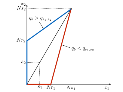
Where here and throughout the paper the overline ()¯¯\overline{()} denotes the average over the random environment. For a fixed direction (s1,s2)+2subscript𝑠1subscript𝑠2superscriptsubscript2(s_{1},s_{2})\in{\mathbb{R}}_{+}^{2} and bulk parameters (γ,β)\gamma,\beta)/(q,q)𝑞superscript𝑞(q,q^{\prime}), our results involves the solution of a saddle-point equation for a boundary parameter λ=λ(s1,s2)𝜆superscript𝜆subscript𝑠1subscript𝑠2\lambda=\lambda^{*}(s_{1},s_{2})/qb=qb(s1,s2)subscript𝑞𝑏superscriptsubscript𝑞𝑏subscript𝑠1subscript𝑠2q_{b}=q_{b}^{*}(s_{1},s_{2}). Based on some unproven ‘natural’ assumptions of convexity and regularity for fIB(s1,s2)subscript𝑓IBsubscript𝑠1subscript𝑠2f_{{\rm IB}}(s_{1},s_{2}) and 𝖿BG(s1,s2)subscript𝖿BGsubscript𝑠1subscript𝑠2{\sf f}_{{\rm BG}}(s_{1},s_{2}) we obtain:

fIB(s1,s2)=s1(ψ(β+λ)+ψ(γλ))+s2(ψ(β+λ)+ψ(λ)),subscript𝑓IBsubscript𝑠1subscript𝑠2subscript𝑠1𝜓𝛽superscript𝜆𝜓𝛾superscript𝜆subscript𝑠2𝜓𝛽superscript𝜆𝜓superscript𝜆\displaystyle f_{{\rm IB}}(s_{1},s_{2})=s_{1}\left(-\psi(\beta+\lambda^{*})+\psi(\gamma-\lambda^{*})\right)+s_{2}\left(-\psi(\beta+\lambda^{*})+\psi(\lambda^{*})\right)\ , (III.38)
0=s1(ψ(β+λ)ψ(γλ))+s2(ψ(β+λ)+ψ(λ)),0subscript𝑠1superscript𝜓𝛽superscript𝜆superscript𝜓𝛾superscript𝜆subscript𝑠2superscript𝜓𝛽superscript𝜆superscript𝜓superscript𝜆\displaystyle 0=s_{1}\left(-\psi^{\prime}(\beta+\lambda^{*})-\psi^{\prime}(\gamma-\lambda^{*})\right)+s_{2}\left(-\psi^{\prime}(\beta+\lambda^{*})+\psi^{\prime}(\lambda^{*})\right)\ , (III.39)

where ψ=Γ/Γ𝜓superscriptΓΓ\psi=\Gamma^{\prime}/\Gamma is the diGamma function and with the condition 0<λ(s1,s2)<γ0superscript𝜆subscript𝑠1subscript𝑠2𝛾0<\lambda^{*}(s_{1},s_{2})<\gamma for the IB polymer, and

𝖿BG(s1,s2)=(q(qb)2q)(qqb)(qbq1)s1+qb(q1)(qb1)(qbq1)s2,subscript𝖿BGsubscript𝑠1subscript𝑠2𝑞superscriptsuperscriptsubscript𝑞𝑏2superscript𝑞𝑞superscriptsubscript𝑞𝑏superscriptsubscript𝑞𝑏superscript𝑞1subscript𝑠1superscriptsubscript𝑞𝑏superscript𝑞1superscriptsubscript𝑞𝑏1superscriptsubscript𝑞𝑏superscript𝑞1subscript𝑠2\displaystyle{\sf f}_{{\rm BG}}(s_{1},s_{2})=-\frac{\left(q-\left(q_{b}^{*}\right)^{2}q^{\prime}\right)}{\left(q-q_{b}^{*}\right)\left(q_{b}^{*}q^{\prime}-1\right)}s_{1}+\frac{q_{b}^{*}\left(q^{\prime}-1\right)}{\left(q_{b}^{*}-1\right)\left(q_{b}^{*}q^{\prime}-1\right)}s_{2}\ , (III.40)
(qb1)2(q(qb)2(q)2+(q24qbq+(qb)2)q+q)s1(qqb)2(q1)((qb)2q1)s2=0,superscriptsuperscriptsubscript𝑞𝑏12𝑞superscriptsuperscriptsubscript𝑞𝑏2superscriptsuperscript𝑞2superscript𝑞24superscriptsubscript𝑞𝑏𝑞superscriptsuperscriptsubscript𝑞𝑏2superscript𝑞𝑞subscript𝑠1superscript𝑞superscriptsubscript𝑞𝑏2superscript𝑞1superscriptsuperscriptsubscript𝑞𝑏2superscript𝑞1subscript𝑠20\displaystyle\left(q_{b}^{*}-1\right)^{2}\left(q\left(q_{b}^{*}\right)^{2}\left(q^{\prime}\right)^{2}+\left(q^{2}-4q_{b}^{*}q+\left(q_{b}^{*}\right)^{2}\right)q^{\prime}+q\right)s_{1}-\left(q-q_{b}^{*}\right)^{2}\left(q^{\prime}-1\right)\left(\left(q_{b}^{*}\right)^{2}q^{\prime}-1\right)s_{2}=0\ , (III.41)

with the condition q<qb(s1,s2)<1𝑞superscriptsubscript𝑞𝑏subscript𝑠1subscript𝑠21q<q_{b}^{*}(s_{1},s_{2})<1 for the BG polymer.

Note that while (III.39) is a transcendental equation for λ(s1,s2)superscript𝜆subscript𝑠1subscript𝑠2\lambda^{*}(s_{1},s_{2}), (III.41) is a quartic equation for qb(s1,s2)superscriptsubscript𝑞𝑏subscript𝑠1subscript𝑠2q_{b}^{*}(s_{1},s_{2}), which can be solved explicitly using radicals. These results cannot be considered as mathematical theorems since they rely on unproven assumptions (which could likely be proven by other means). Still, their derivation is very close to a mathematical proof. We note that the result (III.38) for fIB(s1,s2)subscript𝑓IBsubscript𝑠1subscript𝑠2f_{{\rm IB}}(s_{1},s_{2}) coincides with the result obtained in Eq.(79)-(81) in usIBeta 222there cφ=fIB(1/2+φ,1/2φ)subscript𝑐𝜑subscript𝑓IB12𝜑12𝜑c_{\varphi}=f_{{\rm IB}}(1/2+\varphi,1/2-\varphi) for φ]1/2,1/2[\varphi\in]-1/2,1/2[ and the equivalent of λsuperscript𝜆\lambda^{*} there is the saddle-point parameter kφ=γ/2+λsubscript𝑘𝜑𝛾2superscript𝜆k_{\varphi}=\gamma/2+\lambda^{*} using non-rigorous replica calculations, and the above result thus gives a close to rigorous confirmation of one conjecture of usIBeta .

Optimal angles
Of interest are the optimal angles φopt]1/2,1/2[\varphi_{{\rm opt}}\in]-1/2,1/2[, the ‘angles’ for which the mean quenched free-energy/optimal energy per unit length in the direction φ]1/2,1/2[\varphi\in]-1/2,1/2[, defined as

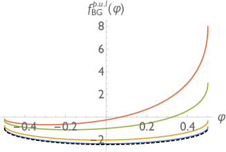
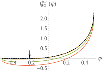
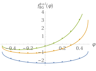
fIBp.u.l.(φ)=fIB(1/2+φ,1/2φ),𝖿BGp.u.l.φ)=𝖿IB(1/2+φ,1/2φ),\displaystyle f^{{\rm p.u.l.}}_{{\rm IB}}(\varphi)=f_{{\rm IB}}(1/2+\varphi,1/2-\varphi)\quad,\quad{\sf f}^{{\rm p.u.l.}}_{{\rm BG}}\varphi)={\sf f}_{{\rm IB}}(1/2+\varphi,1/2-\varphi)\ , (III.42)

are maximum. These quantities are non-trivial in these anisotropic models and we obtain the explicit formulas

φoptIB=12ψ(β+γ/2)ψ(γ/2)0,φoptBG=(q1)2q2(qq1)20.\displaystyle\varphi_{{\rm opt}}^{{\rm IB}}=-\frac{1}{2}\frac{\psi^{\prime}(\beta+\gamma/2)}{\psi^{\prime}(\gamma/2)}\leq 0\quad,\quad\varphi_{{\rm opt}}^{{\rm BG}}=-\frac{\left(\sqrt{q}-1\right)^{2}q^{\prime}}{2\left(\sqrt{q}q^{\prime}-1\right)^{2}}\leq 0\ . (III.43)

These angles would correspond to the mean direction chosen by the polymer for a point to line polymer problem. The formula for φoptIBsuperscriptsubscript𝜑optIB\varphi_{{\rm opt}}^{{\rm IB}} was already given in Eq.(83) of usIBeta .

III.4 Convergence of point to point models to their stationary state

Finally, based on the upon results, we conjecture that the following limits in law holds: (Lu,Lv)2for-allsubscript𝐿𝑢subscript𝐿𝑣superscript2\forall(L_{u},L_{v})\in{\mathbb{N}}^{2} and (s1,s2)+2subscript𝑠1subscript𝑠2superscriptsubscript2(s_{1},s_{2})\in{\mathbb{R}}_{+}^{2}

limN(ZNs1+x1,Ns2+x2ZNs1,Ns2)0x1Lu,0x2Lv(Z^x1,x2)0x1Lu,0x2Lvsimilar-tosubscript𝑁subscriptsubscript𝑍𝑁subscript𝑠1subscript𝑥1𝑁subscript𝑠2subscript𝑥2subscript𝑍𝑁subscript𝑠1𝑁subscript𝑠2formulae-sequence0subscript𝑥1subscript𝐿𝑢0subscript𝑥2subscript𝐿𝑣subscriptsubscript^𝑍subscript𝑥1subscript𝑥2formulae-sequence0subscript𝑥1subscript𝐿𝑢0subscript𝑥2subscript𝐿𝑣\displaystyle\lim_{N\to\infty}\left(\frac{Z_{Ns_{1}+x_{1},Ns_{2}+x_{2}}}{Z_{Ns_{1},Ns_{2}}}\right)_{0\leq x_{1}\leq L_{u},0\leq x_{2}\leq L_{v}}\sim\left(\hat{Z}_{x_{1},x_{2}}\right)_{0\leq x_{1}\leq L_{u},0\leq x_{2}\leq L_{v}} (III.44)
limN(𝖤Ns1+x1,Ns2+x2𝖤Ns1,Ns2)0x1Lu,0x2Lv(𝖤^x1,x2)0x1Lu,0x2Lvsimilar-tosubscript𝑁subscriptsubscript𝖤𝑁subscript𝑠1subscript𝑥1𝑁subscript𝑠2subscript𝑥2subscript𝖤𝑁subscript𝑠1𝑁subscript𝑠2formulae-sequence0subscript𝑥1subscript𝐿𝑢0subscript𝑥2subscript𝐿𝑣subscriptsubscript^𝖤subscript𝑥1subscript𝑥2formulae-sequence0subscript𝑥1subscript𝐿𝑢0subscript𝑥2subscript𝐿𝑣\displaystyle\lim_{N\to\infty}\left({\sf E}_{Ns_{1}+x_{1},Ns_{2}+x_{2}}-{\sf E}_{Ns_{1},Ns_{2}}\right)_{0\leq x_{1}\leq L_{u},0\leq x_{2}\leq L_{v}}\sim\left(\hat{\sf E}_{x_{1},x_{2}}\right)_{0\leq x_{1}\leq L_{u},0\leq x_{2}\leq L_{v}} (III.45)

where the left hand sides of these limits involve the point to point partition sum/optimal energy in the IB/BG polymer, and the right hand sides involve the corresponding quantities in the models with boundaries with boundary parameters λ=λ(s1,s2)𝜆superscript𝜆subscript𝑠1subscript𝑠2\lambda=\lambda^{*}(s_{1},s_{2}) and qb=qb(s1,s2)subscript𝑞𝑏superscriptsubscript𝑞𝑏subscript𝑠1subscript𝑠2q_{b}=q_{b}^{*}(s_{1},s_{2}), the solutions of the equations (III.39) and (III.41).

III.5 Outline and some additional results not presented here

The outline of the remaining of this manuscript is as follows. In Sec. IV and V we prove the stationarity and reversibility properties of the Inverse-Beta and Bernoulli-Geometric polymers of Sec. III.2, and discuss the connections between our work and previous works. In Sec. VI.1 we obtain results for the asymptotic mean quenched free-energy and mean optimal energy in the IB and BG polymers with boundaries, and using these results we obtain in Sec. VI.2 the corresponding formulas (III.38)-(III.40) for the point to point models. In Sec. VI.3 we discuss the conjectures for the convergence of both models to their stationary measure (III.44)-(III.45). In Sec. VI.4 we briefly discuss the nature of the fluctuations of the free-energy in the models with boundaries. Finally in Sec. VII we perform some simulations of the BG polymer and check our result and conjecture (III.40) and (III.45) for this newly introduced model.

IV Finite-temperature model: stationary measure of the Inverse-Beta polymer

In this section we show the stationarity properties of the IB polymer of Sec. III.2.1. We follow closely the approach developed by Seppäläinen for the case of the Log-Gamma polymer Seppalainen2012 and adapt it to the Inverse-Beta polymer. We also discuss the connection between out work and previous works.

IV.1 Stationary property of the model with boundaries

We begin by showing the stationarity property Prop. III.1 of the IB model with boundaries (see Def. III.2). First, note that in the bulk of 2superscript2{\mathbb{N}}^{2}, i.e. for x1,x21subscript𝑥1subscript𝑥21x_{1},x_{2}\geq 1, the partition sum Z^x1,x2subscript^𝑍subscript𝑥1subscript𝑥2\hat{Z}_{x_{1},x_{2}} satisfies the bulk recursion

Z^x1,x2=ux1,x2Z^x11,x2+vx1,x2Z^x1,x21forx1,x21.formulae-sequencesubscript^𝑍subscript𝑥1subscript𝑥2subscript𝑢subscript𝑥1subscript𝑥2subscript^𝑍subscript𝑥11subscript𝑥2subscript𝑣subscript𝑥1subscript𝑥2subscript^𝑍subscript𝑥1subscript𝑥21forsubscript𝑥1subscript𝑥21\displaystyle\hat{Z}_{x_{1},x_{2}}=u_{x_{1},x_{2}}\hat{Z}_{x_{1}-1,x_{2}}+v_{x_{1},x_{2}}\hat{Z}_{x_{1},x_{2}-1}\quad\text{for}\hskip 2.84544ptx_{1},x_{2}\geq 1\ . (IV.1)

This implies that the vertical and horizontal ratios of partition sums U^x1,x2subscript^𝑈subscript𝑥1subscript𝑥2\hat{U}_{x_{1},x_{2}} and V^x1,x2subscript^𝑉subscript𝑥1subscript𝑥2\hat{V}_{x_{1},x_{2}} defined in (III.26) satisfy the following recursion relation, valid for x1,x21subscript𝑥1subscript𝑥21x_{1},x_{2}\geq 1,

U^x1,x2=ϕ(1)(U^x1,x21,V^x11,x2,Wx1,x2),V^x1,x2=ϕ(2)(U^x1,x21,V^x11,x2,Wx1,x2) ,\displaystyle\hat{U}_{x_{1},x_{2}}=\phi^{(1)}(\hat{U}_{x_{1},x_{2}-1},\hat{V}_{x_{1}-1,x_{2}},W_{x_{1},x_{2}})\quad,\quad\hat{V}_{x_{1},x_{2}}=\phi^{(2)}(\hat{U}_{x_{1},x_{2}-1},\hat{V}_{x_{1}-1,x_{2}},W_{x_{1},x_{2}}) \ , (IV.2)

where ϕ(i)superscriptitalic-ϕ𝑖\phi^{(i)} denotes the ithsuperscript𝑖𝑡i^{th} component of the image of the stationarity-reversibility map ϕitalic-ϕ\phi that we now define.

Definition IV.1.

The stationarity-reversibility map is the function ϕ:(U,V,W)()3(U,V,W)()3:italic-ϕ𝑈𝑉𝑊superscriptsuperscript3superscript𝑈superscript𝑉superscript𝑊superscriptsuperscript3\phi:(U,V,W)\in({\mathbb{R}}^{*})^{3}\to(U^{\prime},V^{\prime},W^{\prime})\in({\mathbb{R}}^{*})^{3} defined by

U=W+(W+1)UV,V=WVU+W+1,W=U(V1)U+V.\displaystyle U^{\prime}=W+(W+1)\frac{U}{V}\quad,\quad V^{\prime}=W\frac{V}{U}+W+1\quad,\quad W^{\prime}=\frac{U(V-1)}{U+V}\ .\ (IV.3)

It has the following properties:

Proposition IV.1.

Stationarity If (U,V,W)𝑈𝑉𝑊(U,V,W) are three independent RVs distributed as in (III.2) and (III.3), then (U,V,W):=ϕ(U,V,W)assignsuperscript𝑈superscript𝑉superscript𝑊italic-ϕ𝑈𝑉𝑊(U^{\prime},V^{\prime},W^{\prime}):=\phi(U,V,W) are three independent RVs distributed as in (III.2) and (III.3).

Proposition IV.2.

Reversibility ϕitalic-ϕ\phi is an involution, i.e. ϕϕ=Iditalic-ϕitalic-ϕ𝐼𝑑\phi\circ\phi=Id.

These properties are proved in Appendix. A. Based on the above properties of ϕitalic-ϕ\phi, the stationarity property of the model with boundary conditions Prop. III.1 is proved by induction on the set of down-right paths (see Def. III.7) on 2superscript2{\mathbb{N}}^{2}. We first need a definition:

Definition IV.2.

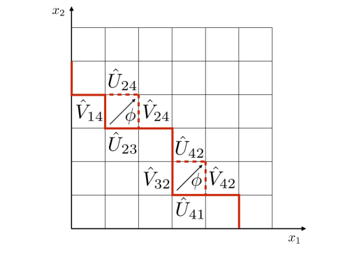
Down-left to top-right transformation on down-right paths A down-right path πdr2subscript𝜋𝑑𝑟2\pi_{dr2} is a ‘down-left to top-right’ (henceforth: DLTR) transformed down-right path of a down-right path πdr2subscript𝜋𝑑𝑟2\pi_{dr2} if πdr2subscript𝜋𝑑𝑟2\pi_{dr2} can be obtained from πdr1subscript𝜋𝑑𝑟1\pi_{dr1} by a transformation where edges of πdr1subscript𝜋𝑑𝑟1\pi_{dr1} forming a down-left corner, i.e. of the form (x1,x2)(x1,x21)(x+1,x21)subscript𝑥1subscript𝑥2subscript𝑥1subscript𝑥21𝑥1subscript𝑥21(x_{1},x_{2})\to(x_{1},x_{2}-1)\to(x+1,x_{2}-1)), are replaced in πdr2subscript𝜋𝑑𝑟2\pi_{dr2} by the two edges forming the corresponding top-right corner (x1,x2)(x1+1,x2)(x1+1,x21)subscript𝑥1subscript𝑥2subscript𝑥11subscript𝑥2subscript𝑥11subscript𝑥21(x_{1},x_{2})\to(x_{1}+1,x_{2})\to(x_{1}+1,x_{2}-1) (see Fig. 5).

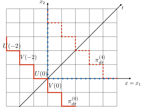
Let us now give the proof of the stationarity property Prop. III.1 of the model with boundary conditions. First, note that the stationarity property is trivially true for the down-right paths that follow exactly the boundaries of 2superscript2\mathbb{N}^{2} (since on these down-right paths the RVs U^x1,x2subscript^𝑈subscript𝑥1subscript𝑥2\hat{U}_{x_{1},x_{2}} and V^x1,x2subscript^𝑉subscript𝑥1subscript𝑥2\hat{V}_{x_{1},x_{2}} are just the random Boltzmann weights on the boundaries Ux1,0subscript𝑈subscript𝑥10U_{x_{1},0} and V0,x2subscript𝑉0𝑥2V_{0,x2} which are independent and distributed as (III.2)). Let us now suppose that the stationarity property Prop. III.1 is true for a down right path πdr1subscript𝜋𝑑𝑟1\pi_{dr1} such that πdr1subscript𝜋𝑑𝑟1\pi_{dr1} contains one couple of edges of the form (x1,x2)(x1,x21)(x+1,x21)subscript𝑥1subscript𝑥2subscript𝑥1subscript𝑥21𝑥1subscript𝑥21(x_{1},x_{2})\to(x_{1},x_{2}-1)\to(x+1,x_{2}-1) (i.e. it contains two edges forming a down-left corner, see Fig. 5). The vertical edge then carries the RV V^x1,x2subscript^𝑉subscript𝑥1subscript𝑥2\hat{V}_{x_{1},x_{2}} and the horizontal edge carries the RV U^x1+1,x21subscript^𝑈subscript𝑥11subscript𝑥21\hat{U}_{x_{1}+1,x_{2}-1}. Applying the induction (IV.2) on this couple of edges, we obtain the couple of RVs (U^x1+1,x2,V^x1+1,x2)subscript^𝑈subscript𝑥11subscript𝑥2subscript^𝑉subscript𝑥11subscript𝑥2(\hat{U}_{x_{1}+1,x_{2}},\hat{V}_{x_{1}+1,x_{2}}). These RVs, complemented by the other RVs U^x1,x2subscript^𝑈superscriptsubscript𝑥1superscriptsubscript𝑥2\hat{U}_{x_{1}^{\prime},x_{2}^{\prime}} and V^x1,x2subscript^𝑉superscriptsubscript𝑥1superscriptsubscript𝑥2\hat{V}_{x_{1}^{\prime},x_{2}^{\prime}} that live on πdr1subscript𝜋𝑑𝑟1\pi_{dr1} and were left untouched by this induction, now live on a down right path πdr2subscript𝜋𝑑𝑟2\pi_{dr2} defined such that the edges visited by πdr2subscript𝜋𝑑𝑟2\pi_{dr2} are exactly those visited by πdr1subscript𝜋𝑑𝑟1\pi_{dr1} except for the couple of edges (x1,x2)(x1,x21)(x+1,x21)subscript𝑥1subscript𝑥2subscript𝑥1subscript𝑥21𝑥1subscript𝑥21(x_{1},x_{2})\to(x_{1},x_{2}-1)\to(x+1,x_{2}-1) that is replaced by (x1,x2)(x1+1,x2)(x1+1,x21)subscript𝑥1subscript𝑥2subscript𝑥11subscript𝑥2subscript𝑥11subscript𝑥21(x_{1},x_{2})\to(x_{1}+1,x_{2})\to(x_{1}+1,x_{2}-1) (see Fig. 5). Using the stationarity property of ϕitalic-ϕ\phi Prop. IV.1 one concludes that those RVs satisfy the stationarity property Prop. III.1. Hence the DLTR transformation on down-right paths conserves the stationarity property, and we will generally think of the variables (U,V)𝑈𝑉(U,V) (resp. (U,V)superscript𝑈superscript𝑉(U^{\prime},V^{\prime})) in (IV.3) as living on down-left (resp. top right) corners (see Fig. 5). Finally, since any down-right path on 2superscript2\mathbb{N}^{2} can be obtained from a down-right path that follows exactly the edges of 2superscript2\mathbb{N}^{2} by a sequence of DLTR transformations, the stationarity property holds for any down-right path on 2superscript2{\mathbb{N}}^{2}. In this sense, the stationarity property of the model with boundaries can be thought of as a propagation of boundary conditions.
Refer to caption

Figure 5: Red: a down-right path on 2superscript2\mathbb{N}^{2}. Red-dashed: a new possible down-right path obtained from the first one by transforming two down-left corners into two top-rights ones (resulting from two down-left to top-right transformations, see Def. IV.2). The RVs U^x1,x2subscript^𝑈subscript𝑥1subscript𝑥2\hat{U}_{x_{1},x_{2}} and V^x1,x2subscript^𝑉subscript𝑥1subscript𝑥2\hat{V}_{x_{1},x_{2}} on the new down-right path are either the same as for the first path, or obtained from those on the first path using the stationarity-reversibility map ϕitalic-ϕ\phi through the induction (IV.2).

IV.2 Stationarity property of the model with stationary initial condition

We now consider the IB with stationary initial condition defined in Def. III.3. Similarly as before, the horizontal and vertical ratios of partition sums Uˇt(x)subscriptˇ𝑈𝑡𝑥\check{U}_{t}(x) and Vˇt(x)subscriptˇ𝑉𝑡𝑥\check{V}_{t}(x) (defined in (III.27)) satisfy the following recursion equation, valid for t0𝑡0t\geq 0 and x𝑥x\in{\mathbb{Z}}

Uˇt+1(x)=ϕ(1)(Uˇt(x),Vˇt(x1),Wt+1(x)),Vˇt+1(x)=ϕ(2)(Uˇt(x),Vˇt(x1),Wt+1(x)).\displaystyle\check{U}_{t+1}(x)=\phi^{(1)}(\check{U}_{t}(x),\check{V}_{t}(x-1),W_{t+1}(x))\quad,\quad\check{V}_{t+1}(x)=\phi^{(2)}(\check{U}_{t}(x),\check{V}_{t}(x-1),W_{t+1}(x))\ . (IV.4)

In this model, the stationary initial condition (III.10) is designed to provide an initial down right path on 2superscript2\mathbb{Z}^{2},

πdr(0)={(x1,x2)=(m,m)(m,m1)(m+1,m1),m}\displaystyle\pi_{dr}^{(0)}=\{(x_{1},x_{2})=(m,-m)\to(m,-m-1)\to(m+1,-m-1),m\in\mathbb{Z}\} (IV.5)

on which the variable Uˇt(x)subscriptˇ𝑈𝑡𝑥\check{U}_{t}(x) and Vˇt(x)subscriptˇ𝑉𝑡𝑥\check{V}_{t}(x) defined in (III.27) are all independent and distributed as in (III.2), (see Fig. 6). Starting from this initial down-right path and successively applying DLTR transformations as described previously, one obtains the following improved (compared to Prop. III.2) stationarity property.

Proposition IV.3.

Improved Stationarity property of the model with stationary initial condition On each down-right path πdrsubscript𝜋𝑑𝑟\pi_{dr} on 2superscript2\mathbb{Z}^{2} that can be obtained from πdr(0)superscriptsubscript𝜋𝑑𝑟0\pi_{dr}^{(0)} by a sequence of DLTR transformations, the variables Uˇt(x)subscriptˇ𝑈𝑡𝑥\check{U}_{t}(x) and Vˇt(x)subscriptˇ𝑉𝑡𝑥\check{V}_{t}(x) that live on πdrsubscript𝜋𝑑𝑟\pi_{dr} are independent and distributed as in (III.2).

For concreteness let us highlight some down-right paths that can be obtained from πdr(0)superscriptsubscript𝜋𝑑𝑟0\pi_{dr}^{(0)} using DLTR transformations (see left of Fig. 6) and prove the properties Prop. III.2 and Prop. III.4. These includes

1) For all t1𝑡1t\geq 1 the down-right path

πdr(t)={(x1,x2)=(t+m,m)(t+m,m1)(t+m+1,m1),m}\displaystyle\pi_{dr}^{(t)}=\{(x_{1},x_{2})=(t+m,-m)\to(t+m,-m-1)\to(t+m+1,-m-1),m\in\mathbb{Z}\} (IV.6)

In particular this implies the stationarity property Prop. III.2. Note that this shows that in the model with stationary initial condition, for all t1𝑡1t\geq 1, the RVs {Yˇt(x):=Zˇt(x+1)/Zˇt(x),x}formulae-sequenceassignsubscriptˇ𝑌𝑡𝑥subscriptˇ𝑍𝑡𝑥1subscriptˇ𝑍𝑡𝑥𝑥\{\check{Y}_{t}(x):=\check{Z}_{t}(x+1)/\check{Z}_{t}(x),x\in\mathbb{Z}\} are iid and distributed as U/V𝑈𝑉U/V with U𝑈U and V𝑉V distributed as in (III.2). This stationarity property for the Yˇt(x)subscriptˇ𝑌𝑡𝑥\check{Y}_{t}(x) variables has the advantage of only involving partition sums at the same time coordinate t𝑡t. It is trivially implied by the stronger property of stationarity of Uˇt(x)subscriptˇ𝑈𝑡𝑥\check{U}_{t}(x) and Vˇt(x)subscriptˇ𝑉𝑡𝑥\check{V}_{t}(x) on down-right paths and we will focus on the latter in the following.

2) The boundary of 2superscript2\mathbb{N}^{2}, which is itself a down-right path, can also be obtained from πdr(0)superscriptsubscript𝜋𝑑𝑟0\pi_{dr}^{(0)}. This shows that on the boundaries of 2superscript2{\mathbb{N}}^{2}, the partition sums in the IB polymer with stationary initial condition Zˇx1,x2subscriptˇ𝑍subscript𝑥1subscript𝑥2\check{Z}_{x_{1},x_{2}} and in the model with boundary conditions Z^x1,x2subscript^𝑍subscript𝑥1subscript𝑥2\hat{Z}_{x_{1},x_{2}} are equivalent in law. Since the partition sums in these models in the remaining of 2superscript2{\mathbb{N}}^{2} are uniquely determined by their values on the boundaries and by the random BWs in the bulk of 2superscript2{\mathbb{N}}^{2}, which coincide in both models, we obtain Prop. III.4, i.e. (Zˇx1,x2)(x1,x2)2(Z^x1,x2)(x1,x2)2similar-tosubscriptsubscriptˇ𝑍subscript𝑥1subscript𝑥2subscript𝑥1subscript𝑥2superscript2subscriptsubscript^𝑍subscript𝑥1subscript𝑥2subscript𝑥1subscript𝑥2superscript2(\check{Z}_{x_{1},x_{2}})_{(x_{1},x_{2})\in{\mathbb{N}}^{2}}\sim(\hat{Z}_{x_{1},x_{2}})_{(x_{1},x_{2})\in{\mathbb{N}}^{2}}.

Refer to caption Refer to caption

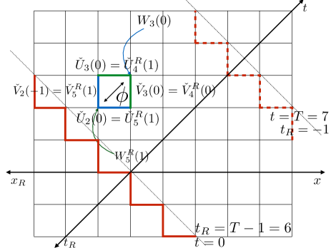
Figure 6: Left: Stationary measure of the Inverse-Beta polymer with stationary initial condition. The initial down right path πdr(0)superscriptsubscript𝜋𝑑𝑟0\pi_{dr}^{(0)} on which the initial condition is defined carries RVs Uˇt=0(x)=U(x)subscriptˇ𝑈𝑡0𝑥𝑈𝑥\check{U}_{t=0}(x)=U(x) and Vˇt=0(x)=V(x)subscriptˇ𝑉𝑡0𝑥𝑉𝑥\check{V}_{t=0}(x)=V(x) for which the stationarity property holds. Any down-right paths obtained from πdr(0)superscriptsubscript𝜋𝑑𝑟0\pi_{dr}^{(0)} by down-left to top-right transformations then carries RVs Uˇt(x)subscriptˇ𝑈𝑡𝑥\check{U}_{t}(x) and Vˇt(x)subscriptˇ𝑉𝑡𝑥\check{V}_{t}(x) such that the stationarity property holds. These include e.g. all down-right paths πdr(t)superscriptsubscript𝜋𝑑𝑟𝑡\pi_{dr}^{(t)} for t0𝑡0t\geq 0 (such as πdr(4)superscriptsubscript𝜋𝑑𝑟4\pi_{dr}^{(4)} in dashed-red above) and the boundaries of 2superscript2\mathbb{N}^{2} (in dotted blue above). Right: Illustration of the symmetry between the forward and time-reversed process for T=7𝑇7T=7. In the time evolution of the forward process, the RVs Uˇ2(0)subscriptˇ𝑈20\check{U}_{2}(0) and Vˇ2(1)subscriptˇ𝑉21\check{V}_{2}(-1) (on the blue edges above) are transformed using ϕitalic-ϕ\phi into the RVs Uˇ3(0)subscriptˇ𝑈30\check{U}_{3}(0) and Vˇ3(0)subscriptˇ𝑉30\check{V}_{3}(0) (on the green edges above) using the random Boltzmann weight W3(0)subscript𝑊30W_{3}(0). From this evolution one stores, using ϕitalic-ϕ\phi the random Boltzmann weights W5R(1)superscriptsubscript𝑊5𝑅1W_{5}^{R}(1) later used in the time evolution of the backward process where the RVs Uˇ4R(1)superscriptsubscriptˇ𝑈4𝑅1\check{U}_{4}^{R}(1) and Vˇ4R(0)superscriptsubscriptˇ𝑉4𝑅0\check{V}_{4}^{R}(0) (on the green edges above) are evolved using ϕitalic-ϕ\phi into the RVs Uˇ5R(1)superscriptsubscriptˇ𝑈5𝑅1\check{U}_{5}^{R}(1) and Vˇ5R(1)superscriptsubscriptˇ𝑉5𝑅1\check{V}_{5}^{R}(1).

Remarks

  • The condition Zˇ0(0)=1subscriptˇ𝑍001\check{Z}_{0}(0)=1 in the initial condition (III.10) is arbitrary and could be replaced by any other constant or RV as long as it is independent of the variable U(x)𝑈𝑥U(x) and V(x)𝑉𝑥V(x). The equality in law between the model with stationary initial condition in the upper right quadrant and the model with boundary conditions then more generally reads (Zˇx1,x2/Zˇ0,0)(x1,x2)2(Z^x1,x2)(x1,x2)2similar-tosubscriptsubscriptˇ𝑍subscript𝑥1subscript𝑥2subscriptˇ𝑍00subscript𝑥1subscript𝑥2superscript2subscriptsubscript^𝑍subscript𝑥1subscript𝑥2subscript𝑥1subscript𝑥2superscript2(\check{Z}_{x_{1},x_{2}}/\check{Z}_{0,0})_{(x_{1},x_{2})\in{\mathbb{N}}^{2}}\sim(\hat{Z}_{x_{1},x_{2}})_{(x_{1},x_{2})\in{\mathbb{N}}^{2}}.

  • Here we have thus obtained a family (indexed by λ𝜆\lambda) of stationary measures for the Inverse-Beta polymer. These correspond to discrete random walks at fixed t𝑡t as a function of x𝑥x for the free energy logZˇt(x)subscriptˇ𝑍𝑡𝑥-\log\check{Z}_{t}(x). We will see in the following that these random walks have generally a non-zero drift, except in the ‘equilibrium case’ λ=γ/2𝜆𝛾2\lambda=\gamma/2. This discrete stationary measure is thus a natural generalization of the stationary measure of the continuum DP, or equivalently of the 111 dimensional KPZ equation HuseHenleyFisher ; ForsterNelsonStephen . Note also that as in the continuum case, the stationary measure only concerns quotients of partition sums/differences of free-energies and the one-point distribution of Zˇt(0)subscriptˇ𝑍𝑡0\check{Z}_{t}(0) is not stationary. Hence the full process (Zˇt(x))t=0,,T;xsubscriptsubscriptˇ𝑍𝑡𝑥formulae-sequence𝑡0𝑇𝑥(\check{Z}_{t}(x))_{t=0,\dots,T;x\in\mathbb{Z}}, which can be equivalently parametrized by the couple (Zˇt(x=0),(Uˇt(x),Vˇt(x))t=0,,T;x)subscriptˇ𝑍𝑡𝑥0subscriptsubscriptˇ𝑈𝑡𝑥subscriptˇ𝑉𝑡𝑥formulae-sequence𝑡0𝑇𝑥\left(\check{Z}_{t}(x=0),(\check{U}_{t}(x),\check{V}_{t}(x))_{t=0,\dots,T;x\in\mathbb{Z}}\right) is not stationary, but the process we are studying however (Uˇt(x),Vˇt(x))t=0,,T;xsubscriptsubscriptˇ𝑈𝑡𝑥subscriptˇ𝑉𝑡𝑥formulae-sequence𝑡0𝑇𝑥(\check{U}_{t}(x),\check{V}_{t}(x))_{t=0,\dots,T;x\in\mathbb{Z}}, is a marginal of the latter and is stationary.

IV.3 Reversibility of the stationary measure: detailed balance property

We now discuss the reversibility of the stationary process. We first study reversibility at the level of a DLTR transformation on down-right paths, then at the level of the process (Uˇt(x),Vˇt(x))xsubscriptsubscriptˇ𝑈𝑡𝑥subscriptˇ𝑉𝑡𝑥𝑥(\check{U}_{t}(x),\check{V}_{t}(x))_{x\in{\mathbb{Z}}} and prove the property Prop. III.3.

IV.3.1 At the level of a down-left to top-right transformation

We now show a detailed-balance property for the stationary measure, namely that, if (U,V,W)𝑈𝑉𝑊(U,V,W) are distributed as in (III.2) and (III.3) and (U,V,W)=ϕ(U,V,W)superscript𝑈superscript𝑉superscript𝑊italic-ϕ𝑈𝑉𝑊(U^{\prime},V^{\prime},W^{\prime})=\phi(U,V,W), then the PDF of the couples of couples of RVS P((U,V);(U,V))𝑃superscript𝑈superscript𝑉𝑈𝑉P((U^{\prime},V^{\prime});(U,V)) is symmetric by exchange (U,V)(U,V)𝑈𝑉superscript𝑈superscript𝑉(U,V)\leftrightarrow(U^{\prime},V^{\prime}). Indeed, let us consider ((U,V);(U,V))superscript𝑈superscript𝑉𝑈𝑉((U^{\prime},V^{\prime});(U,V)) fixed and note Pstat(U,V,W)=PU(U)PV(V)PW(W)subscript𝑃𝑠𝑡𝑎𝑡𝑈𝑉𝑊subscript𝑃𝑈𝑈subscript𝑃𝑉𝑉subscript𝑃𝑊𝑊P_{stat}(U,V,W)=P_{U}(U)P_{V}(V)P_{W}(W) the stationary PDF of the triplet of RVs in (IV.3) (see (III.3) and (III.2) for the expressions of PU(U)subscript𝑃𝑈𝑈P_{U}(U), PV(V)subscript𝑃𝑉𝑉P_{V}(V) and PW(W)subscript𝑃𝑊𝑊P_{W}(W)). We have

P((U,V);(U,V))𝑃superscript𝑈superscript𝑉𝑈𝑉\displaystyle P((U^{\prime},V^{\prime});(U,V)) =𝑑Wδ(Uϕ(1)(U,V,W))δ(Vϕ(2)(U,V,W))Pstat(U,V,W)absentdifferential-d𝑊𝛿superscript𝑈superscriptitalic-ϕ1𝑈𝑉𝑊𝛿superscript𝑉superscriptitalic-ϕ2𝑈𝑉𝑊subscript𝑃𝑠𝑡𝑎𝑡𝑈𝑉𝑊\displaystyle=\int dW\delta(U^{\prime}-\phi^{(1)}(U,V,W))\delta(V^{\prime}-\phi^{(2)}(U,V,W))P_{stat}(U,V,W)
=𝑑W𝑑U′′𝑑V′′𝑑W′′δ(Uϕ(1)(U,V,W))δ(Vϕ(2)(U,V,W))absentdifferential-d𝑊differential-dsuperscript𝑈′′differential-dsuperscript𝑉′′differential-dsuperscript𝑊′′𝛿superscript𝑈superscriptitalic-ϕ1𝑈𝑉𝑊𝛿superscript𝑉superscriptitalic-ϕ2𝑈𝑉𝑊\displaystyle=\int dW\int dU^{\prime\prime}dV^{\prime\prime}dW^{\prime\prime}\delta(U^{\prime}-\phi^{(1)}(U,V,W))\delta(V^{\prime}-\phi^{(2)}(U,V,W))
δ(3)((U,V,W)ϕ(U′′,V′′,W′′))Pstat(U′′,V′′,W′′)UNKNOWNsuperscript𝛿3𝑈𝑉𝑊italic-ϕsuperscript𝑈′′superscript𝑉′′superscript𝑊′′subscript𝑃𝑠𝑡𝑎𝑡superscript𝑈′′superscript𝑉′′superscript𝑊′′UNKNOWN\displaystyle\quad\quad\quad\quad\quad\quad\delta^{(3)}((U,V,W)-\phi(U^{\prime\prime},V^{\prime\prime},W^{\prime\prime}))P_{stat}(U^{\prime\prime},V^{\prime\prime},W^{\prime\prime}) 
=𝑑W𝑑U′′𝑑V′′𝑑W′′δ(UU′′)δ(VV′′)absentdifferential-d𝑊differential-dsuperscript𝑈′′differential-dsuperscript𝑉′′differential-dsuperscript𝑊′′𝛿superscript𝑈superscript𝑈′′𝛿superscript𝑉superscript𝑉′′\displaystyle=\int dW\int dU^{\prime\prime}dV^{\prime\prime}dW^{\prime\prime}\delta(U^{\prime}-U^{\prime\prime})\delta(V^{\prime}-V^{\prime\prime})
δ(3)((U,V,W)ϕ(U′′,V′′,W′′))Pstat(U′′,V′′,W′′)UNKNOWNsuperscript𝛿3𝑈𝑉𝑊italic-ϕsuperscript𝑈′′superscript𝑉′′superscript𝑊′′subscript𝑃𝑠𝑡𝑎𝑡superscript𝑈′′superscript𝑉′′superscript𝑊′′UNKNOWN\displaystyle\quad\quad\quad\quad\quad\quad\delta^{(3)}((U,V,W)-\phi(U^{\prime\prime},V^{\prime\prime},W^{\prime\prime}))P_{stat}(U^{\prime\prime},V^{\prime\prime},W^{\prime\prime}) 
=𝑑W′′δ(Uϕ(1)(U′′,V′′,W′′))δ(Vϕ(2)(U′′,V′′,W′′))Pstat(U′′,V′′,W′′)absentdifferential-dsuperscript𝑊′′𝛿𝑈superscriptitalic-ϕ1superscript𝑈′′superscript𝑉′′superscript𝑊′′𝛿𝑉superscriptitalic-ϕ2superscript𝑈′′superscript𝑉′′superscript𝑊′′subscript𝑃𝑠𝑡𝑎𝑡superscript𝑈′′superscript𝑉′′superscript𝑊′′\displaystyle=\int dW^{\prime\prime}\delta(U-\phi^{(1)}(U^{\prime\prime},V^{\prime\prime},W^{\prime\prime}))\delta(V-\phi^{(2)}(U^{\prime\prime},V^{\prime\prime},W^{\prime\prime}))P_{stat}(U^{\prime\prime},V^{\prime\prime},W^{\prime\prime})
P((U,V);(U,V))absent𝑃superscript𝑈superscript𝑉𝑈𝑉\displaystyle\Longrightarrow P((U^{\prime},V^{\prime});(U,V)) =P((U,V);(U,V))absent𝑃𝑈𝑉superscript𝑈superscript𝑉\displaystyle=P((U,V);(U^{\prime},V^{\prime})) (IV.9)

which is the desired detailed balance property. Here we have successively used that ϕitalic-ϕ\phi preserves the PDF Pstat(U,V,W)subscript𝑃𝑠𝑡𝑎𝑡𝑈𝑉𝑊P_{stat}(U,V,W) (in (IV.3.1)) and that ϕitalic-ϕ\phi is an involution (in (IV.3.1)). This property can also be rewritten in the more usual form, using that P((U,V);(U,V))=P((U,V)|(U,V))Pstat(U,V)𝑃superscript𝑈superscript𝑉𝑈𝑉𝑃conditionalsuperscript𝑈superscript𝑉𝑈𝑉subscript𝑃𝑠𝑡𝑎𝑡𝑈𝑉P((U^{\prime},V^{\prime});(U,V))=P((U^{\prime},V^{\prime})|(U,V))P_{stat}(U,V), with Pstat(U,V)=PU(U)PV(V)subscript𝑃𝑠𝑡𝑎𝑡𝑈𝑉subscript𝑃𝑈𝑈subscript𝑃𝑉𝑉P_{stat}(U,V)=P_{U}(U)P_{V}(V) the stationary PDF of the couple of RVs (U,V)𝑈𝑉(U,V),

P((U,V)|(U,V))P((U,V)|(U,V))=Pstat(U,V)Pstat(U,V).𝑃conditionalsuperscript𝑈superscript𝑉𝑈𝑉𝑃conditional𝑈𝑉superscript𝑈superscript𝑉subscript𝑃𝑠𝑡𝑎𝑡superscript𝑈superscript𝑉subscript𝑃𝑠𝑡𝑎𝑡𝑈𝑉\displaystyle\frac{P((U^{\prime},V^{\prime})|(U,V))}{P((U,V)|(U^{\prime},V^{\prime}))}=\frac{P_{stat}(U^{\prime},V^{\prime})}{P_{stat}(U,V)}\ . (IV.10)

From a more pragmatical point of view, the above detailed balance property can also be proven using direct calculations. One easily obtains from (IV.3) and (III.2) that

P((U,V)|(U,V))=Γ(γ+β)Γ(γ)Γ(β)(V(UVUVU+V)β(U+VVU+V)γ)(VUU)δ(VUVU)θ(U>0)θ(V>1),𝑃conditionalsuperscript𝑈superscript𝑉𝑈𝑉Γ𝛾𝛽Γ𝛾Γ𝛽𝑉superscript𝑈𝑉superscript𝑈𝑉superscript𝑈𝑉𝛽superscript𝑈𝑉𝑉superscript𝑈𝑉𝛾𝑉superscript𝑈𝑈𝛿superscript𝑉superscript𝑈𝑉𝑈𝜃𝑈0𝜃𝑉1\displaystyle P((U^{\prime},V^{\prime})|(U,V))=\frac{\Gamma(\gamma+\beta)}{\Gamma(\gamma)\Gamma(\beta)}\frac{\left(V\left(-\frac{U-VU^{\prime}}{VU^{\prime}+V}\right)^{\beta}\left(\frac{U+V}{VU^{\prime}+V}\right)^{\gamma}\right)}{\left(VU^{\prime}-U\right)}\delta\left(V^{\prime}-\frac{U^{\prime}V}{U}\right)\theta(U>0)\theta(V>1)\ , (IV.11)

and Eq. (IV.10) can then directly be checked.

IV.3.2 At the level of the full space-time process

We now give two proofs of the property Prop. III.2, with the first only relying on the detailed balance property (IV.10) and which will be useful for the BG polymer case. We remind the reader that on a finite time interval t[0,T]𝑡0𝑇t\in[0,T] with T𝑇superscriptT\in{\mathbb{N}}^{*}, the time-reversed coordinates are defined as (see (III.28)) tR=Tt1subscript𝑡𝑅𝑇𝑡1t_{R}=T-t-1 and xR=xsubscript𝑥𝑅𝑥x_{R}=-x. The stationary forward process is defined by drawing a random environment (Wt(x))t=1,,T,xsubscriptsubscript𝑊𝑡𝑥formulae-sequence𝑡1𝑇𝑥(W_{t}(x))_{t=1,\dots,T,x\in\mathbb{Z}} according to (III.3), an initial condition (U^t=0(x),V^t=0(x))subscript^𝑈𝑡0𝑥subscript^𝑉𝑡0𝑥(\hat{U}_{t=0}(x),\hat{V}_{t=0}(x)) according to the stationary measure (III.2), and let it deterministically evolve using (IV.4). The time-reversed process was defined for tR[0,T]subscript𝑡𝑅0𝑇t_{R}\in[0,T] in (III.29) as

UˇtRR(xR)=Uˇt=TtR(x=xR+1),VˇtRR(xR)=Vˇt=TtR(x=xR).\displaystyle\check{U}_{t_{R}}^{R}(x_{R})=\check{U}_{t=T-t_{R}}(x=-x_{R}+1)\quad,\quad\check{V}_{t_{R}}^{R}(x_{R})=\check{V}_{t=T-t_{R}}(x=-x_{R})\ . (IV.12)

Let us first comment on this definition. First note the shift by one unity of the x𝑥x coordinate in the definition of UˇtR(xR)subscriptˇ𝑈subscript𝑡𝑅subscript𝑥𝑅\check{U}_{t_{R}}(x_{R}) compared to VˇtRR(xR)superscriptsubscriptˇ𝑉subscript𝑡𝑅𝑅subscript𝑥𝑅\check{V}_{t_{R}}^{R}(x_{R}). The reason for this is that, in the forward evolution, ϕitalic-ϕ\phi mixes up RVs (U,V)𝑈𝑉(U,V) living on edges leading to different vertices (forming a down-left corner) and creates RVs (U,V)superscript𝑈superscript𝑉(U^{\prime},V^{\prime}) living on edges leading to the same vertex (forming a top-right corner) (see (IV.4)). In the time-reversed process the Usuperscript𝑈U^{\prime} and Vsuperscript𝑉V^{\prime} RVs are then reinterpreted as living on edges leading to different vertices (forming a down-left corner in the (tR,xR)subscript𝑡𝑅subscript𝑥𝑅(t_{R},x_{R}) coordinates) whereas the RVs U𝑈U and V𝑉V live on edges leading to the same vertex (forming a top-right corner in the (tR,xR)subscript𝑡𝑅subscript𝑥𝑅(t_{R},x_{R}) coordinates). The shift by one unity of the t𝑡t coordinate in the definition of UˇtR(xR)subscriptˇ𝑈subscript𝑡𝑅subscript𝑥𝑅\check{U}_{t_{R}}(x_{R}) and VˇtRR(xR)superscriptsubscriptˇ𝑉subscript𝑡𝑅𝑅subscript𝑥𝑅\check{V}_{t_{R}}^{R}(x_{R}) (compared to (III.28)) ensures that the final values at t=T𝑡𝑇t=T of the forward process are initial values at tR=0subscript𝑡𝑅0t_{R}=0 for the backward process. This is illustrated on the right of Fig. 6. Introducing these notations permits to rewrite the detailed balance condition (IV.9) as

P((Uˇt+1(x),Vˇt+1(x)),(Uˇt(x),Vˇt(x1)))𝑃subscriptˇ𝑈𝑡1𝑥subscriptˇ𝑉𝑡1𝑥subscriptˇ𝑈𝑡𝑥subscriptˇ𝑉𝑡𝑥1\displaystyle P\left((\check{U}_{t+1}(x),\check{V}_{t+1}(x)),(\check{U}_{t}(x),\check{V}_{t}(x-1))\right) =P((Uˇt(x),Vˇt(x1)),(Uˇt+1(x),Vˇt+1(x)))absent𝑃subscriptˇ𝑈𝑡𝑥subscriptˇ𝑉𝑡𝑥1subscriptˇ𝑈𝑡1𝑥subscriptˇ𝑉𝑡1𝑥\displaystyle=P\left((\check{U}_{t}(x),\check{V}_{t}(x-1)),(\check{U}_{t+1}(x),\check{V}_{t+1}(x))\right) (IV.13)
=P((UˇtR+1R(xR),VˇtR+1R(xR)),(UˇtRR(xR),VˇtRR(xR1)))absent𝑃subscriptsuperscriptˇ𝑈𝑅subscript𝑡𝑅1subscript𝑥𝑅subscriptsuperscriptˇ𝑉𝑅subscript𝑡𝑅1subscript𝑥𝑅subscriptsuperscriptˇ𝑈𝑅subscript𝑡𝑅subscript𝑥𝑅subscriptsuperscriptˇ𝑉𝑅subscript𝑡𝑅subscript𝑥𝑅1\displaystyle=P\left((\check{U}^{R}_{t_{R}+1}(x_{R}),\check{V}^{R}_{t_{R}+1}(x_{R})),(\check{U}^{R}_{t_{R}}(x_{R}),\check{V}^{R}_{t_{R}}(x_{R}-1))\right)\

(here we used that the process is homogeneous and stationary). Using inductively (IV.13) (and using that the measure is stationary and that the RVs Uˇt(x)subscriptˇ𝑈𝑡𝑥\check{U}_{t}(x) and Vˇt(x)subscriptˇ𝑉𝑡𝑥\check{V}_{t}(x) at different position x𝑥x are independent) shows the equality in law stated in Prop. III.3 between the forward and time-reversed process. Another way to understand this reversibility property is to explicitly construct a random environment in which the reversed process performs a forward evolution. In this case we use the stronger (compared to the detailed balance property (IV.9)) property of reversibility of ϕitalic-ϕ\phi Prop. IV.2:

  1. 1.

    Start from a drawing of a random environment (Wt(x))t=1,,T,xsubscriptsubscript𝑊𝑡𝑥formulae-sequence𝑡1𝑇𝑥(W_{t}(x))_{t=1,\dots,T,x\in\mathbb{Z}} distributed as in (III.3) and of the variables (Uˇt=0(x),Vˇt=0(x))subscriptˇ𝑈𝑡0𝑥subscriptˇ𝑉𝑡0𝑥(\check{U}_{t=0}(x),\check{V}_{t=0}(x)) distributed according to the stationary measure (III.2).

  2. 2.

    Evolve (Uˇt(x),Vˇt(x))subscriptˇ𝑈𝑡𝑥subscriptˇ𝑉𝑡𝑥(\check{U}_{t}(x),\check{V}_{t}(x)) from t=0𝑡0t=0 to t=T𝑡𝑇t=T according to (IV.4). At each time step, store also a new disorder RV as, for 1trT1subscript𝑡𝑟𝑇1\leq t_{r}\leq T,

    WtRR(xR)=ϕ(3)(Uˇt(x),Vˇt(x1),Wt+1(x))|t=TtR,x=xR+1.subscriptsuperscript𝑊𝑅subscript𝑡𝑅subscript𝑥𝑅evaluated-atsuperscriptitalic-ϕ3subscriptˇ𝑈𝑡𝑥subscriptˇ𝑉𝑡𝑥1subscript𝑊𝑡1𝑥formulae-sequence𝑡𝑇subscript𝑡𝑅𝑥subscript𝑥𝑅1\displaystyle W^{R}_{t_{R}}(x_{R})=\phi^{(3)}(\check{U}_{t}(x),\check{V}_{t}(x-1),W_{t+1}(x))|_{t=T-t_{R},x=-x_{R}+1}\ . (IV.14)
  3. 3.

    Then, using that ϕitalic-ϕ\phi is an involution (Prop. IV.2) shows that the backward process satisfies

    UˇtR+1R(xR)=ϕ(1)(UˇtRR(x),VˇtRR(x1),WtR+1R(x)),VˇtR+1R(x)=ϕ(2)(UˇtRR(x),VˇtRR(xR1),WtR+1R(xR)),\check{U}^{R}_{t_{R}+1}(x_{R})=\phi^{(1)}(\check{U}^{R}_{t_{R}}(x),\check{V}^{R}_{t_{R}}(x-1),W^{R}_{t_{R}+1}(x))\quad,\quad\check{V}^{R}_{t_{R}+1}(x)=\phi^{(2)}(\check{U}^{R}_{t_{R}}(x),\check{V}^{R}_{t_{R}}(x_{R}-1),W^{R}_{t_{R}+1}(x_{R}))\ , (IV.15)

    that is, the backward process satisfies a forward evolution in the random environment WtRR(xR)subscriptsuperscript𝑊𝑅subscript𝑡𝑅subscript𝑥𝑅W^{R}_{t_{R}}(x_{R}), which is, using the properties of ϕitalic-ϕ\phi, a legitimate Inverse-Beta random environment (i.e. the WtRR(xR)subscriptsuperscript𝑊𝑅subscript𝑡𝑅subscript𝑥𝑅W^{R}_{t_{R}}(x_{R}) are independent and distributed as (III.3) and are independent of the stationary initial condition (UˇtT=0R(xR),VˇtR=0R(xR))subscriptsuperscriptˇ𝑈𝑅subscript𝑡𝑇0subscript𝑥𝑅subscriptsuperscriptˇ𝑉𝑅subscript𝑡𝑅0subscript𝑥𝑅(\check{U}^{R}_{t_{T}=0}(x_{R}),\check{V}^{R}_{t_{R}=0}(x_{R}))).

This shows in a more constructive fashion that the backward process in indistinguishable from a forward process and that the equality in law (III.30) holds. This procedure is illustrated on the right of Fig. 6. Note finally that if the RVs in the reversed process are interpreted as quotients of time-reversed partition sums ZˇtRR(xR)subscriptsuperscriptˇ𝑍𝑅subscript𝑡𝑅subscript𝑥𝑅\check{Z}^{R}_{t_{R}}(x_{R}), we must have by definition

UˇtRR(xR)=ZˇtRR(xR)ZˇtR1R(xR1)=UˇTtR(xR+1)=ZˇTtR(xR+1)ZˇTtR1(xR),subscriptsuperscriptˇ𝑈𝑅subscript𝑡𝑅subscript𝑥𝑅subscriptsuperscriptˇ𝑍𝑅subscript𝑡𝑅subscript𝑥𝑅subscriptsuperscriptˇ𝑍𝑅subscript𝑡𝑅1subscript𝑥𝑅1subscriptˇ𝑈𝑇subscript𝑡𝑅subscript𝑥𝑅1subscriptˇ𝑍𝑇subscript𝑡𝑅subscript𝑥𝑅1subscriptˇ𝑍𝑇subscript𝑡𝑅1subscript𝑥𝑅\displaystyle\check{U}^{R}_{t_{R}}(x_{R})=\frac{\check{Z}^{R}_{t_{R}}(x_{R})}{\check{Z}^{R}_{t_{R}-1}(x_{R}-1)}=\check{U}_{T-t_{R}}(-x_{R}+1)=\frac{\check{Z}_{T-t_{R}}(-x_{R}+1)}{\check{Z}_{T-t_{R}-1}(-x_{R})}\ ,
VˇtRR(xR)=ZˇtRR(xR)ZˇtR1R(xR)=VˇTtR(xR)=ZˇTtR(xR)ZˇTtR1(xR),subscriptsuperscriptˇ𝑉𝑅subscript𝑡𝑅subscript𝑥𝑅subscriptsuperscriptˇ𝑍𝑅subscript𝑡𝑅subscript𝑥𝑅subscriptsuperscriptˇ𝑍𝑅subscript𝑡𝑅1subscript𝑥𝑅subscriptˇ𝑉𝑇subscript𝑡𝑅subscript𝑥𝑅subscriptˇ𝑍𝑇subscript𝑡𝑅subscript𝑥𝑅subscriptˇ𝑍𝑇subscript𝑡𝑅1subscript𝑥𝑅\displaystyle\check{V}^{R}_{t_{R}}(x_{R})=\frac{\check{Z}^{R}_{t_{R}}(x_{R})}{\check{Z}^{R}_{t_{R}-1}(x_{R})}=\check{V}_{T-t_{R}}(-x_{R})=\frac{\check{Z}_{T-t_{R}}(-x_{R})}{\check{Z}_{T-t_{R}-1}(-x_{R})}\ ,\ (IV.16)

and an appropriate definition of ZˇtRR(xR)subscriptsuperscriptˇ𝑍𝑅subscript𝑡𝑅subscript𝑥𝑅\check{Z}^{R}_{t_{R}}(x_{R}) is thus

ZˇtRR(xR):=1ZˇTtR1(xR).assignsubscriptsuperscriptˇ𝑍𝑅subscript𝑡𝑅subscript𝑥𝑅1subscriptˇ𝑍𝑇subscript𝑡𝑅1subscript𝑥𝑅\displaystyle\check{Z}^{R}_{t_{R}}(x_{R}):=\frac{1}{\check{Z}_{T-t_{R}-1}(-x_{R})}\ . (IV.17)

Alternatively one can multiply this definition by a constant term as ZˇtRR(xR):=ZˇT1(0)/ZˇTtR1(xR)assignsubscriptsuperscriptˇ𝑍𝑅subscript𝑡𝑅subscript𝑥𝑅subscriptˇ𝑍𝑇10subscriptˇ𝑍𝑇subscript𝑡𝑅1subscript𝑥𝑅\check{Z}^{R}_{t_{R}}(x_{R}):=\check{Z}_{T-1}(0)/\check{Z}_{T-t_{R}-1}(-x_{R}) to ensure the initial condition ZˇtRR(0)=1subscriptsuperscriptˇ𝑍𝑅subscript𝑡𝑅01\check{Z}^{R}_{t_{R}}(0)=1 as well. In this case one has in law (Zˇt(x))t=0,,T;x(ZˇtRR(xR))tR=0,,T;xRsimilar-tosubscriptsubscriptˇ𝑍𝑡𝑥formulae-sequence𝑡0𝑇𝑥subscriptsubscriptsuperscriptˇ𝑍𝑅subscript𝑡𝑅subscript𝑥𝑅formulae-sequencesubscript𝑡𝑅0𝑇subscript𝑥𝑅(\check{Z}_{t}(x))_{t=0,\dots,T;x\in\mathbb{Z}}\sim(\check{Z}^{R}_{t_{R}}(x_{R}))_{t_{R}=0,\dots,T;x_{R}\in\mathbb{Z}}.

IV.4 Relation to other models

In this section we explicitly consider the implication of our results for the Log-Gamma and Stric-Weak polymers, two exactly solvable models of DPs on 2superscript2{\mathbb{Z}}^{2} that can be obtained as limits of the IB polymer. We will not discuss here the 00 temperature limits (γ,β)(0,0)𝛾𝛽00(\gamma,\beta)\to(0,0), whose discussion is reported to Sec. V.2. We will use here the language of polymers with boundaries to discuss the stationary measures.

IV.4.1 Limit to the Log-Gamma polymer

In usIBeta it was shown that the point-to-point partition-sum of the Inverse-Beta polymer (without boundaries) converges to the partition-sum of the Log-Gamma polymer as

limβZx1,x2βx1+x2=Zx1,x2LG,subscript𝛽subscript𝑍subscript𝑥1subscript𝑥2superscript𝛽subscript𝑥1subscript𝑥2subscriptsuperscript𝑍𝐿𝐺subscript𝑥1subscript𝑥2\displaystyle\lim_{\beta\to\infty}\frac{Z_{x_{1},x_{2}}}{\beta^{x_{1}+x_{2}}}=Z^{LG}_{x_{1},x_{2}}\ , (IV.18)

where the limit holds in law and Zx1,x2LGsuperscriptsubscript𝑍subscript𝑥1subscript𝑥2𝐿𝐺Z_{x_{1},x_{2}}^{LG} is the partition sum of the Log-Gamma polymer. The latter is defined as in Def. III.1 but in this case the random variables are distributed as uLG=vLGsuperscript𝑢𝐿𝐺superscript𝑣𝐿𝐺u^{LG}=v^{LG} and (uLG)1superscriptsuperscript𝑢𝐿𝐺1(u^{LG})^{-1} is distributed as a Gamma distribution with parameter γ>0𝛾0\gamma>0333Here uLG=vLGsuperscript𝑢𝐿𝐺superscript𝑣𝐿𝐺u^{LG}=v^{LG} means that the random Boltzmann weights can equally well be interpreted as living on the vertices of the square lattice. At the level of the random Boltzmann weights the convergence in law reads

(uβ,vβ)(1Beta(γ,β)βBeta(γ,β),1βBeta(γ,β))β(uLG,vLG)(1,1)Gamma(γ).similar-to𝑢𝛽𝑣𝛽1𝐵𝑒𝑡𝑎𝛾𝛽𝛽𝐵𝑒𝑡𝑎𝛾𝛽1𝛽𝐵𝑒𝑡𝑎𝛾𝛽subscriptsimilar-to𝛽superscript𝑢𝐿𝐺superscript𝑣𝐿𝐺similar-to11𝐺𝑎𝑚𝑚𝑎𝛾\displaystyle\left(\frac{u}{\beta},\frac{v}{\beta}\right)\sim\left(\frac{1-Beta(\gamma,\beta)}{\beta Beta(\gamma,\beta)},\frac{1}{\beta Beta(\gamma,\beta)}\right)\sim_{\beta\to\infty}(u^{LG},v^{LG})\sim\frac{(1,1)}{Gamma(\gamma)}. (IV.19)

In the same way, using (III.2), (III.3), a stationary Log-Gamma polymer with boundaries is obtained as

Z^x1,x2LG=limβZ^x1,x2βx1+x2,subscriptsuperscript^𝑍𝐿𝐺subscript𝑥1subscript𝑥2subscript𝛽subscript^𝑍subscript𝑥1subscript𝑥2superscript𝛽subscript𝑥1subscript𝑥2\displaystyle\hat{Z}^{LG}_{x_{1},x_{2}}=\lim_{\beta\to\infty}\frac{\hat{Z}_{x_{1},x_{2}}}{\beta^{x_{1}+x_{2}}}\ ,
ULG=limβ Uβ(Gamma(γλ))1,superscript𝑈𝐿𝐺subscript𝛽 𝑈𝛽similar-tosuperscript𝐺𝑎𝑚𝑚𝑎𝛾𝜆1\displaystyle U^{LG}=\lim_{\beta\to\infty} \frac{U}{\beta}\sim\left(Gamma(\gamma-\lambda)\right)^{-1}\ ,
VLG=limβ Vβ(Gamma(λ))1,superscript𝑉𝐿𝐺subscript𝛽 𝑉𝛽similar-tosuperscript𝐺𝑎𝑚𝑚𝑎𝜆1\displaystyle V^{LG}=\lim_{\beta\to\infty} \frac{V}{\beta}\sim\left(Gamma(\lambda)\right)^{-1}\ ,
WLG=limβ Wβ(Gamma(γ))1,superscript𝑊𝐿𝐺subscript𝛽 𝑊𝛽similar-tosuperscript𝐺𝑎𝑚𝑚𝑎𝛾1\displaystyle W^{LG}=\lim_{\beta\to\infty} \frac{W}{\beta}\sim\left(Gamma(\gamma)\right)^{-1}\ , (IV.20)

(all these limits hold in law). Here Z^x1,x2LGsubscriptsuperscript^𝑍𝐿𝐺subscript𝑥1𝑥2\hat{Z}^{LG}_{x_{1},x2} is the partition sum of the Log-Gamma polymer with boundaries defined as for the IB polymer with boundaries (see Def III.2) with random BWs distributed as Ux1,0ULGsimilar-tosubscript𝑈subscript𝑥10superscript𝑈𝐿𝐺U_{x_{1},0}\sim U^{LG}, V0,x2VLGsimilar-tosubscript𝑉0subscript𝑥2superscript𝑉𝐿𝐺V_{0,x_{2}}\sim V^{LG} and ux1,x2=vx1,x2WLGsubscript𝑢subscript𝑥1subscript𝑥2subscript𝑣subscript𝑥1subscript𝑥2similar-tosuperscript𝑊𝐿𝐺u_{x_{1},x_{2}}=v_{x_{1},x_{2}}\sim W^{LG}. This is the same model as introduced in Seppalainen2012 and our results of stationarity in the IB polymer imply the results Lemma 3.2 and Theorem 3.3 of Seppalainen2012 .

IV.4.2 Limit to the Strict-Weak polymer

In usIBeta it was shown that the point-to-point partition-sum of the Inverse-Beta polymer converges to the partition-sum of the Strict-Weak polymer without boundaries as

limγγx1Zx1,x2=Zx1,x2SW,subscript𝛾superscript𝛾subscript𝑥1subscript𝑍subscript𝑥1subscript𝑥2subscriptsuperscript𝑍𝑆𝑊subscript𝑥1subscript𝑥2\displaystyle\lim_{\gamma\to\infty}\gamma^{x_{1}}Z_{x_{1},x_{2}}=Z^{SW}_{x_{1},x_{2}}\ , (IV.21)

where the limit holds in law and Zx1,x2SWsuperscriptsubscript𝑍subscript𝑥1subscript𝑥2𝑆𝑊Z_{x_{1},x_{2}}^{SW} is the partition sum of the Strict-Weak polymer. It is defined as in Def. III.1 but in this case the random variables are distributed as vSW=1superscript𝑣𝑆𝑊1v^{SW}=1 and uSWsuperscript𝑢𝑆𝑊u^{SW} is distributed with a Gamma distribution of parameter β>0𝛽0\beta>0. At the level of the random Boltzmann weights the convergence in law reads

(γu,v)(γ(1Beta(γ,β))Beta(γ,β),1Beta(γ,β))γ(uSW,vSW)(Gamma(β),1).similar-to𝛾𝑢𝑣𝛾1𝐵𝑒𝑡𝑎𝛾𝛽𝐵𝑒𝑡𝑎𝛾𝛽1𝐵𝑒𝑡𝑎𝛾𝛽subscriptsimilar-to𝛾superscript𝑢𝑆𝑊superscript𝑣𝑆𝑊similar-to𝐺𝑎𝑚𝑚𝑎𝛽1\displaystyle(\gamma u,v)\sim\left(\frac{\gamma(1-Beta(\gamma,\beta))}{Beta(\gamma,\beta)},\frac{1}{Beta(\gamma,\beta)}\right)\sim_{\gamma\to\infty}(u^{SW},v^{SW})\sim\left(Gamma(\beta),1\right)\ . (IV.22)

A stationary Strict-Weak polymer with boundaries is similarly obtained as, using (III.2) and (III.3),

Z^x1,x2SW=limγγx1Z^x1,x2,subscriptsuperscript^𝑍𝑆𝑊subscript𝑥1subscript𝑥2subscript𝛾superscript𝛾subscript𝑥1subscript^𝑍subscript𝑥1subscript𝑥2\displaystyle\hat{Z}^{SW}_{x_{1},x_{2}}=\lim_{\gamma\to\infty}\gamma^{x_{1}}\hat{Z}_{x_{1},x_{2}}\ ,
USW=limγ γUGamma(β+λ),superscript𝑈𝑆𝑊subscript𝛾 𝛾𝑈similar-to𝐺𝑎𝑚𝑚𝑎𝛽𝜆\displaystyle U^{SW}=\lim_{\gamma\to\infty} \gamma U\sim Gamma(\beta+\lambda)\ ,
VSW=limγ V(Beta(λ,β))1,superscript𝑉𝑆𝑊subscript𝛾 𝑉similar-tosuperscript𝐵𝑒𝑡𝑎𝜆𝛽1\displaystyle V^{SW}=\lim_{\gamma\to\infty} V\sim\left(Beta(\lambda,\beta)\right)^{-1}\ ,
WSW=limγ γWGamma(β),superscript𝑊𝑆𝑊subscript𝛾 𝛾𝑊similar-to𝐺𝑎𝑚𝑚𝑎𝛽\displaystyle W^{SW}=\lim_{\gamma\to\infty} \gamma W\sim Gamma(\beta)\ , (IV.23)

(all these limits hold in law). Here Z^x1,x2SWsubscriptsuperscript^𝑍𝑆𝑊subscript𝑥1subscript𝑥2\hat{Z}^{SW}_{x_{1},x_{2}} is the partition sum of the stationary Strict-Weak polymer with boundaries defined as for the IB polymer with boundaries with random BWs distributed as Ux1,0USWsimilar-tosubscript𝑈subscript𝑥10superscript𝑈𝑆𝑊U_{x_{1},0}\sim U^{SW}, V0,x2VSWsimilar-tosubscript𝑉0subscript𝑥2superscript𝑉𝑆𝑊V_{0,x_{2}}\sim V^{SW}, ux1,x2WLGsimilar-tosubscript𝑢subscript𝑥1subscript𝑥2superscript𝑊𝐿𝐺u_{x_{1},x_{2}}\sim W^{LG} and vx1,x2=1subscript𝑣subscript𝑥1subscript𝑥21v_{x_{1},x_{2}}=1. It satisfies stationarity and reversibility properties inherited from those of the IB polymer (see Sec. III.2.1). We note that this stationary Strict-Weak polymer with boundaries differs from the one considered in StrictWeak1 . Indeed, the admissible paths considered in StrictWeak1 differ from ours, and so does the stationarity property there obtained which involve ratios of partition sums slightly different from ours (see Definition 6.1, Proposition 6.2 and Lemma 6.3 in StrictWeak1 ). While these two stationary process are different, we note that the ESPs that underly them are different incarnations of the Beta-Gamma algebra of RVs.

V 00 temperature model: Stationary measure of the Bernoulli-Geometric polymer

In this section we obtain the stationarity properties of the BG polymer with boundary conditions and stationary initial condition stated in Sec. III.2.2 and discuss the link between our results and previous results on other models. Thanks to the notations we used, the proof of these properties will be (almost) completely analogous to the finite temperature case and we will thus give much less details in this section.

V.1 Stationarity properties of the Bernoulli-Geometric polymer

Let us first focus on the case of the BG polymer with boundaries defined in Def. III.5. In the bulk of 2superscript2{\mathbb{N}}^{2}, the optimal energy in the BG polymer with boundaries satisfies the following recursion equation

𝖤^x1,x2=min(𝖤^x11,x2+𝗎x1,x2,𝖤^x1,x21+𝗏x1,x2) for (x1,x2)()2.subscript^𝖤subscript𝑥1subscript𝑥2subscript^𝖤subscript𝑥11subscript𝑥2subscript𝗎subscript𝑥1subscript𝑥2subscript^𝖤subscript𝑥1subscript𝑥21subscript𝗏subscript𝑥1subscript𝑥2 for subscript𝑥1subscript𝑥2superscriptsuperscript2\displaystyle\hat{\sf E}_{x_{1},x_{2}}={\rm\min}\left(\hat{\sf E}_{x_{1}-1,x_{2}}+{\sf u}_{x_{1},x_{2}},\hat{\sf E}_{x_{1},x_{2}-1}+{\sf v}_{x_{1},x_{2}}\right)\text{ for }(x_{1},x_{2})\in({\mathbb{N}}^{*})^{2}\ . (V.1)

This implies the bulk recursion equation for the horizontal and vertical differences of optimal energies (see (III.32))

𝖴^x1,x2=ϕT=0(1)(𝖴^x1,x21,𝖵^x11,x2,𝗎x1,x2,𝗏x1,x2),𝖵^x1,x2=ϕT=0(2)(𝖴^x1,x21,𝖵^x11,x2,𝗎x1,x2,𝗏x1,x2).\hat{\sf U}_{x_{1},x_{2}}=\phi_{T=0}^{(1)}\left(\hat{\sf U}_{x_{1},x_{2}-1},\hat{\sf V}_{x_{1}-1,x_{2}},{\sf u}_{x_{1},x_{2}},{\sf v}_{x_{1},x_{2}}\right)\quad,\quad\hat{\sf V}_{x_{1},x_{2}}=\phi_{T=0}^{(2)}\left(\hat{\sf U}_{x_{1},x_{2}-1},\hat{\sf V}_{x_{1}-1,x_{2}},{\sf u}_{x_{1},x_{2}},{\sf v}_{x_{1},x_{2}}\right)\ . (V.2)

where we have introduced the T=0𝑇0T=0 stationarity map that we now define.

Definition V.1.

The T=0𝑇0T=0 stationarity map ϕT=0subscriptitalic-ϕ𝑇0\phi_{T=0} is the function ϕT=0:(𝖴,𝖵,𝗎,𝗏)4(𝖴,𝖵)2:subscriptitalic-ϕ𝑇0𝖴𝖵𝗎𝗏superscript4superscript𝖴superscript𝖵superscript2\phi_{T=0}:({\sf U},{\sf V},{\sf u},{\sf v})\in{\mathbb{Z}}^{4}\to({\sf U}^{\prime},{\sf V}^{\prime})\in{\mathbb{Z}}^{2} defined by

𝖴=min(𝗎,𝗏+𝖴𝖵),𝖵=min(𝗎+𝖵𝖴,𝗏)=𝖴+𝖵𝖴.\displaystyle{\sf U}^{\prime}={\rm min}\left({\sf u},{\sf v}+{\sf U}-{\sf V}\right)\quad,\quad{\sf V}^{\prime}={\rm min}\left({\sf u}+{\sf V}-{\sf U},{\sf v}\right)={\sf U}^{\prime}+{\sf V}-{\sf U}\ . (V.3)

It has the following properties (below and throughout the rest of the paper perpendicular-to\perp means ‘independent of’):

Proposition V.1.

Stationarity If 𝖴𝖴{\sf U}, 𝖵𝖵{\sf V}, 𝗎𝗎{\sf u} and 𝗏𝗏{\sf v} are RVs distributed as in (III.4) and (III.5) with 𝖴𝖵(𝗎,𝗏)perpendicular-to𝖴𝖵perpendicular-to𝗎𝗏{\sf U}\perp{\sf V}\perp({\sf u},{\sf v}), then the RVs 𝖴superscript𝖴{\sf U}^{\prime}, 𝖵superscript𝖵{\sf V}^{\prime} in (V.3) are distributed as in (III.5) with 𝖴𝖵perpendicular-tosuperscript𝖴superscript𝖵{\sf U}^{\prime}\perp{\sf V}^{\prime}.

Proposition V.2.

Detailed balance If 𝖴𝖴{\sf U}, 𝖵𝖵{\sf V}, 𝗎𝗎{\sf u} and 𝗏𝗏{\sf v} are RVs distributed as in (III.4) and (III.5) with 𝖴𝖵(𝗎,𝗏)perpendicular-to𝖴𝖵perpendicular-to𝗎𝗏{\sf U}\perp{\sf V}\perp({\sf u},{\sf v}) and 𝖴superscript𝖴{\sf U}^{\prime} and 𝖵superscript𝖵{\sf V}^{\prime} are given by (V.3), then

Proba((𝖴,𝖵)=(k𝖴,k𝖵),(𝖴,𝖵)=(k𝖴,k𝖵))=Proba((𝖴,𝖵)=(k𝖴,k𝖵),(𝖴,𝖵)=(k𝖴,k𝖵)).𝑃𝑟𝑜𝑏𝑎formulae-sequencesuperscript𝖴superscript𝖵subscript𝑘superscript𝖴subscript𝑘superscript𝖵𝖴𝖵subscript𝑘𝖴subscript𝑘𝖵𝑃𝑟𝑜𝑏𝑎formulae-sequencesuperscript𝖴superscript𝖵subscript𝑘𝖴subscript𝑘𝖵𝖴𝖵subscript𝑘superscript𝖴subscript𝑘superscript𝖵\displaystyle Proba\left(({\sf U}^{\prime},{\sf V}^{\prime})=(k_{{\sf U}^{\prime}},k_{{\sf V}^{\prime}}),({\sf U},{\sf V})=(k_{{\sf U}},k_{{\sf V}})\right)=Proba\left(({\sf U}^{\prime},{\sf V}^{\prime})=(k_{{\sf U}},k_{{\sf V}}),({\sf U},{\sf V})=(k_{{\sf U}^{\prime}},k_{{\sf V}^{\prime}})\right)\ . (V.4)

These two properties are proved in Appendix B. Thanks to the existence of these properties and of the induction (V.2), the stationarity properties of the BG polymer with boundaries (and similarly of the BG polymer with stationary initial condition) then easily follow as in the previous section by induction on down-right paths.

Remarks

  • Note that contrary to the stationarity-reversibility map ϕitalic-ϕ\phi defined for the Inverse-Beta polymer in Def. IV.1, the stationarity map of the ϕT=0subscriptitalic-ϕ𝑇0\phi_{T=0} model is not an involution. We were not able to extend as before ϕT=0subscriptitalic-ϕ𝑇0\phi_{T=0} to an involution ϕ~T=0:(𝖴,𝖵,𝗎,𝗏)(𝖴,𝖵,𝗎,𝗏):subscript~italic-ϕ𝑇0𝖴𝖵𝗎𝗏superscript𝖴superscript𝖵superscript𝗎superscript𝗏\tilde{\phi}_{T=0}:({\sf U},{\sf V},{\sf u},{\sf v})\to({\sf U}^{\prime},{\sf V}^{\prime},{\sf u}^{\prime},{\sf v}^{\prime}) that conserves the PDF and the independence of 𝖴𝖴{\sf U}, 𝖵𝖵{\sf V} and of the couple (𝗎,𝗏)𝗎𝗏({\sf u},{\sf v}). We believe this is related to the fact that the recursion equation (V.2) ‘loses some memory’, in the sense that if 𝗎x1,x2subscript𝗎subscript𝑥1subscript𝑥2{\sf u}_{x_{1},x_{2}} in (V.2) is too large, its value cannot be inferred from the sole knowledge of 𝖴x1,x2subscript𝖴subscript𝑥1subscript𝑥2{\sf U}_{x_{1},x_{2}} and 𝖵x1,x2subscript𝖵subscript𝑥1subscript𝑥2{\sf V}_{x_{1},x_{2}}. Nevertheless, we were still able to prove the detailed balance property (V.4), which is sufficient to prove the reversibility property of the stationary process Prop. III.7 in the BG polymer with stationary initial condition as for the IB polymer with stationary initial condition: the only difference is that we do not have the explicit construction of the random environment in which the backward process (III.34) satisfies a forward evolution equation.

  • Sets of random variables satisfying a stationarity property similar to the one of the stationarity map (IV.3) have played over the years an important role in the theory of queuing systems since they also provide in this framework models with an exact solvability property. The first occurrence of a property of this type in this context is due to Burke for the case of exponentially distributed RVs Burke . Since then such properties have been designated as Burke properties. Examples of sets of RVs for which Burke properties have been shown notably include systems of Geometric variables OConnell2005 and more recently mixture of Bernoulli and Geometric variables very similar to the ones considered here Martin2009 . The exact solvability property studied in Martin2009 does not however seem trivially connected to the one studied here. From the technical point of view we note that it involves 444 independent Geometric RVs (while our property involves 555), and more conceptually the model studied in Martin2009 naturally corresponds to a problem of first passage percolation, while our model interpolates between problems of first and last passage percolation (see Sec. V.2).

V.2 Relation to other models

Let us now discuss the relations between this model and other known models. We discuss this in the framework of the model with boundaries in order to obtain the stationary measure of the limiting model as well. In the following we will only study the limits at the level of the random energies (𝗎,𝗏,𝖴,𝖵)𝗎𝗏𝖴𝖵({\sf u},{\sf v},{\sf U},{\sf V}). Each limit can be used to define a model equivalent to the BG polymer with boundaries (see Def. III.5) with different distributions of energies in the bulk and on the boundaries and a stationarity property on down-right paths.

V.2.1 q0superscript𝑞0q^{\prime}\to 0 limit: last passage percolation with geometric waiting times

An isotropic limit of the model is obtained by letting q0superscript𝑞0q^{\prime}\to 0. In this case the random energies that enters into the definition of the model with boundaries are distributed as

𝗎gLPP=𝗏gLPP=Gq,superscript𝗎𝑔𝐿𝑃𝑃superscript𝗏𝑔𝐿𝑃𝑃subscript𝐺𝑞\displaystyle{\sf u}^{gLPP}={\sf v}^{gLPP}=-G_{q}\ ,
𝖴gLPP=Gq/qb,superscript𝖴𝑔𝐿𝑃𝑃subscript𝐺𝑞subscript𝑞𝑏\displaystyle{\sf U}^{gLPP}=-G_{q/q_{b}}\ ,
𝖵gLPP=Gqb.superscript𝖵𝑔𝐿𝑃𝑃subscript𝐺subscript𝑞𝑏\displaystyle{\sf V}^{gLPP}=-G_{q_{b}}\ . (V.5)

This model exactly corresponds to geometric last passage percolation as e.g. studied in Johansson2000 for the case without boundaries (note that 𝗎gLPP=𝗏gLPPsuperscript𝗎𝑔𝐿𝑃𝑃superscript𝗏𝑔𝐿𝑃𝑃{\sf u}^{gLPP}={\sf v}^{gLPP} implies that the bulk random energies can be interpreted as living on the vertices of 2superscript2\mathbb{N}^{2}). Indeed, note that while the random energies in the Bernoulli-Geometric polymer can generally be both positive and negative, in this limit the energies are always negative and the energy-minimization problem can be reinterpreted as a maximization problem of the last passage time. The latter is given by 𝖳x1,x2:=𝖤x1,x2=max{eπ𝗍e,π:(0,0)(x1,x2)}assignsubscript𝖳subscript𝑥1subscript𝑥2subscript𝖤subscript𝑥1subscript𝑥2subscript𝑒𝜋subscript𝗍𝑒:𝜋00subscript𝑥1subscript𝑥2{\sf T}_{x_{1},x_{2}}:=-{\sf E}_{x_{1},x_{2}}={\rm\max}\left\{\sum_{e\in\pi}{\sf t}_{e},\pi:(0,0)\to(x_{1},x_{2})\right\}, where the random waiting times on the edges are the opposite of the random energies, 𝗍e:=(e)0assignsubscript𝗍𝑒𝑒0{\sf t}_{e}:=-{\cal E}(e)\geq 0. This model was denoted Geo-LPP in Fig. 1.

V.2.2 q0𝑞0q\to 0 limit: a first passage percolation problem with Geometric waiting times

An anisotropic limit is obtained by letting q0𝑞0q\to 0 with qsuperscript𝑞q^{\prime} fixed. We obtain

(𝗎bgFPP,𝗏bgFPP)=((1ξ𝗎𝗏)(1+Gq),0),superscript𝗎𝑏𝑔𝐹𝑃𝑃superscript𝗏𝑏𝑔𝐹𝑃𝑃1subscript𝜉𝗎𝗏1subscript𝐺superscript𝑞0\displaystyle({\sf u}^{bgFPP},{\sf v}^{bgFPP})=((1-\xi_{{\sf u}{\sf v}})(1+G_{q^{\prime}}),0)\ ,
𝖴bgFPP=(1ξ𝖴)(1+Gqbq),superscript𝖴𝑏𝑔𝐹𝑃𝑃1subscript𝜉𝖴1subscript𝐺subscript𝑞𝑏superscript𝑞\displaystyle{\sf U}^{bgFPP}=(1-\xi_{{\sf U}})(1+G_{q_{b}q^{\prime}})\ ,
𝖵bgFPP=ξVGqb.superscript𝖵𝑏𝑔𝐹𝑃𝑃subscript𝜉𝑉subscript𝐺subscript𝑞𝑏\displaystyle{\sf V}^{bgFPP}=-\xi_{V}G_{q_{b}}\ . (V.6)

with now p𝗎𝗏=1qsubscript𝑝𝗎𝗏1superscript𝑞p_{{\sf u}{\sf v}}=1-q^{\prime}, p𝖴=1qbqsubscript𝑝𝖴1subscript𝑞𝑏superscript𝑞p_{{\sf U}}=1-q_{b}q^{\prime} and p𝖵=1q1qbqsubscript𝑝𝖵1superscript𝑞1subscript𝑞𝑏superscript𝑞p_{{\sf V}}=\frac{1-q^{\prime}}{1-q_{b}q^{\prime}}. Note that in this limit the energies on the (bulk) edges are either 00 (for vertical edges) or positive. Note also that we can replace the bulk energies on horizontal edges by a simple geometric RV since we have the equality in law (1ξ𝗎𝗏)(1+Gq)Gqsimilar-to1subscript𝜉𝗎𝗏1subscript𝐺superscript𝑞subscript𝐺superscript𝑞(1-\xi_{{\sf u}{\sf v}})(1+G_{q^{\prime}})\sim G_{q^{\prime}}. In this limit the optimal energy 𝖤x1,x2subscript𝖤subscript𝑥1subscript𝑥2{{\sf E}}_{x_{1},x_{2}} is thus always the sum of positive terms and the model is naturally interpreted as a model of first passage percolation. Here the first passage time is 𝖳x1,x2:=+𝖤x1,x2=min{eπ𝗍e,π:(0,0)(x1,x2)}assignsubscript𝖳subscript𝑥1subscript𝑥2subscript𝖤subscript𝑥1subscript𝑥2minconditional-setsubscript𝑒𝜋subscript𝗍𝑒𝜋00subscript𝑥1subscript𝑥2{\sf T}_{x_{1},x_{2}}:=+{\sf E}_{x_{1},x_{2}}={\rm min}\left\{\sum_{e\in\pi}{\sf t}_{e},\pi:(0,0)\to(x_{1},x_{2})\right\}, where the random waiting times on the edges are equal to the random energies, 𝗍e:=+(e)0assignsubscript𝗍𝑒𝑒0{\sf t}_{e}:=+{\cal E}(e)\geq 0. This model was denoted Anisotropic Geo-FPP in Fig. 1. This model was already studied in the language of queuing system in OConnell2005 where the authors obtained an analogue Burke property and also showed that the model could be solved exactly using the RSK correspondence.

V.2.3 Continuous limit of the Bernoulli-Geometric polymer and T=0𝑇0T=0 limit of the Inverse-Beta polymer

We now discuss the exponential/continuous limit. It is obtained by letting ϵ0+italic-ϵsuperscript0\epsilon\to 0^{+} with

q=1γϵ,q=1βϵ,qb=1(γλ)ϵ,\displaystyle q=1-\gamma^{\prime}\epsilon\quad,\quad q^{\prime}=1-\beta^{\prime}\epsilon\quad,\quad q_{b}=1-(\gamma^{\prime}-\lambda^{\prime})\epsilon\ , (V.7)

where γ,β>0superscript𝛾superscript𝛽0\gamma^{\prime},\beta^{\prime}>0 and 0<λ<γ0superscript𝜆superscript𝛾0<\lambda^{\prime}<\gamma^{\prime} (to ensure qb>qsubscript𝑞𝑏𝑞q_{b}>q) are three parameters. In this limit the energies have to be rescaled by ϵitalic-ϵ\epsilon and converge in law to exponentially distributed random variables as

(𝗎BExp,𝗏BExp)=ϵ(𝗎,𝗏)ϵ0((1ζ𝗎𝗏)Eβζ𝗎𝗏Eγ,ζ𝗎𝗏Eγ,)\displaystyle({\sf u}^{B-Exp},{\sf v}^{B-Exp})=\epsilon({\sf u},{\sf v})\to_{\epsilon\to 0}((1-\zeta_{{\sf u}{\sf v}})E_{\beta^{\prime}}-\zeta_{{\sf u}{\sf v}}E_{\gamma^{\prime}},-\zeta_{{\sf u}{\sf v}}E_{\gamma^{\prime}},)
𝖴BExp=ϵ𝖴ϵ0(1ζ𝖴)Eβ+λζ𝖴Eγλsuperscript𝖴𝐵𝐸𝑥𝑝italic-ϵ𝖴subscriptitalic-ϵ01subscript𝜁𝖴subscript𝐸superscript𝛽superscript𝜆subscript𝜁𝖴subscript𝐸superscript𝛾superscript𝜆\displaystyle{\sf U}^{B-Exp}=\epsilon{\sf U}\to_{\epsilon\to 0}(1-\zeta_{{\sf U}})E_{\beta^{\prime}+\lambda^{\prime}}-\zeta_{{\sf U}}E_{\gamma^{\prime}-\lambda^{\prime}}
𝖵BExp=ϵ𝖵ϵ0ζ𝖵Eλsuperscript𝖵𝐵𝐸𝑥𝑝italic-ϵ𝖵subscriptitalic-ϵ0subscript𝜁𝖵subscript𝐸superscript𝜆\displaystyle{\sf V}^{B-Exp}=\epsilon{\sf V}\to_{\epsilon\to 0}-\zeta_{{\sf V}}E_{\lambda^{\prime}} (V.8)

where ζ𝗎𝗏subscript𝜁𝗎𝗏\zeta_{{\sf u}{\sf v}}, ζ𝖴subscript𝜁𝖴\zeta_{{\sf U}} and ζ𝖵subscript𝜁𝖵\zeta_{{\sf V}} are Bernoulli RVs with parameters p𝗎𝗏=ββ+γsubscript𝑝𝗎𝗏superscript𝛽superscript𝛽superscript𝛾p_{{\sf u}{\sf v}}=\frac{\beta^{\prime}}{\beta^{\prime}+\gamma^{\prime}}, p𝖴=β+λβ+γsubscript𝑝𝖴superscript𝛽superscript𝜆superscript𝛽superscript𝛾p_{{\sf U}}=\frac{\beta^{\prime}+\lambda^{\prime}}{\beta^{\prime}+\gamma^{\prime}} and p𝖵=ββ+λsubscript𝑝𝖵superscript𝛽superscript𝛽superscript𝜆p_{{\sf V}}=\frac{\beta^{\prime}}{\beta^{\prime}+\lambda^{\prime}} and Eγsubscript𝐸superscript𝛾E_{\gamma^{\prime}}, Eβsubscript𝐸superscript𝛽E_{\beta^{\prime}}, Eγλsubscript𝐸superscript𝛾superscript𝜆E_{\gamma^{\prime}-\lambda^{\prime}}, Eλsubscript𝐸superscript𝜆E_{\lambda^{\prime}} and Eβ+λsubscript𝐸superscript𝛽superscript𝜆E_{\beta^{\prime}+\lambda^{\prime}} denote exponentially distributed RVs. Let us recall here that the PDF of an exponentially distributed RV is

EαExp(α),p(Eα)=αeαEα.\displaystyle E_{\alpha}\sim Exp(\alpha)\quad,\quad p(E_{\alpha})=\alpha e^{-\alpha E_{\alpha}}\ . (V.9)

The optimal energy in this model has to be scaled accordingly as

𝖤^x1,x2BExp=limϵ0ϵ𝖤^x1,x2,subscriptsuperscript^𝖤𝐵𝐸𝑥𝑝subscript𝑥1subscript𝑥2subscriptitalic-ϵ0italic-ϵsubscript^𝖤subscript𝑥1subscript𝑥2\displaystyle\hat{\sf E}^{B-Exp}_{x_{1},x_{2}}=\lim_{\epsilon\to 0}\epsilon\hat{{\sf E}}_{x_{1},x_{2}}, (V.10)

and the results previously obtained in the BG polymer with boundaries also apply to this model using the now exponentially distributed weights (V.2.3). We call this model the Bernoulli-Exponential polymer with boundaries (denoted as Bernoulli-Exp in Fig. 1). This model can also be obtained from the IB polymer with boundaries using γ=ϵγ𝛾italic-ϵsuperscript𝛾\gamma=\epsilon\gamma^{\prime}, β=ϵβ𝛽italic-ϵsuperscript𝛽\beta=\epsilon\beta^{\prime}, λ=ϵλ𝜆italic-ϵsuperscript𝜆\lambda=\epsilon\lambda^{\prime} and scaling the energies as

(𝗎BExp,𝗏BExp)=ϵ(logu,logv)ϵ0((1ζ𝗎𝗏)Eβζ𝗎𝗏Eγ,ζ𝗎𝗏Eγ,),\displaystyle({\sf u}^{B-Exp},{\sf v}^{B-Exp})=-\epsilon(\log u,\log v)\to_{\epsilon\to 0}((1-\zeta_{{\sf u}{\sf v}})E_{\beta^{\prime}}-\zeta_{{\sf u}{\sf v}}E_{\gamma^{\prime}},-\zeta_{{\sf u}{\sf v}}E_{\gamma^{\prime}},)\ ,
𝖴BExp=ϵlogUϵ0(1ζ𝖴)Eβ+λζ𝖴Eγλ,superscript𝖴𝐵𝐸𝑥𝑝italic-ϵ𝑈subscriptitalic-ϵ01subscript𝜁𝖴subscript𝐸superscript𝛽superscript𝜆subscript𝜁𝖴subscript𝐸superscript𝛾superscript𝜆\displaystyle{\sf U}^{B-Exp}=-\epsilon\log U\to_{\epsilon\to 0}(1-\zeta_{{\sf U}})E_{\beta^{\prime}+\lambda^{\prime}}-\zeta_{{\sf U}}E_{\gamma^{\prime}-\lambda^{\prime}}\ ,
𝖵BExp=ϵlogVϵ0ζ𝖵Eλ,superscript𝖵𝐵𝐸𝑥𝑝italic-ϵ𝑉subscriptitalic-ϵ0subscript𝜁𝖵subscript𝐸superscript𝜆\displaystyle{\sf V}^{B-Exp}=-\epsilon\log V\to_{\epsilon\to 0}-\zeta_{{\sf V}}E_{\lambda^{\prime}}\ ,
𝖤^x1,x2BExp=limϵ0ϵlogZ^x1,x2.subscriptsuperscript^𝖤𝐵𝐸𝑥𝑝subscript𝑥1subscript𝑥2subscriptitalic-ϵ0italic-ϵsubscript^𝑍subscript𝑥1subscript𝑥2\displaystyle\hat{\sf E}^{B-Exp}_{x_{1},x_{2}}=\lim_{\epsilon\to 0}-\epsilon\log\hat{Z}_{x_{1},x_{2}}\ . (V.11)

Here the convergence in law of the logarithm of the random Boltzmann weights of the Inverse-Beta polymer to a mixture of Bernoulli and exponential distributions was shown in usIBeta . We refer the reader to usIBeta for the Bethe ansatz study of this polymer model (without boundary conditions) where the authors notably obtain the full distribution of the optimal energy and show Tracy-Widom GUE asymptotic limit. The Bernoulli-Exponential polymer with boundaries has stationarity properties inherited from the stationarity properties of the IB polymer with boundaries, and was first introduced using the limit (V.2.3). The definition of the Bernoulli-Geometric polymer with boundaries Def. III.5 was found by trial and error as a discretization of the Bernoulli-Exponential polymer with boundaries which conserves these stationarity properties (see in particular Appendix B).

Isotropic limit: Exponential last passage percolation 
Note that the Bernoulli-Exponential polymer (V.2.3) admits an isotropic limit βsuperscript𝛽\beta^{\prime}\to\infty which converges to exponential last passage percolation: in this limit

𝗎eLPP=𝗏eLPP=Eγ,superscript𝗎𝑒𝐿𝑃𝑃superscript𝗏𝑒𝐿𝑃𝑃subscript𝐸superscript𝛾\displaystyle{\sf u}^{eLPP}={\sf v}^{eLPP}=-E_{\gamma^{\prime}}\ ,
𝖴eLPP=Eλ,superscript𝖴𝑒𝐿𝑃𝑃subscript𝐸superscript𝜆\displaystyle{\sf U}^{eLPP}=-E_{\lambda^{\prime}}\ ,
𝖵eLPP=Eγλ.superscript𝖵𝑒𝐿𝑃𝑃subscript𝐸superscript𝛾superscript𝜆\displaystyle{\sf V}^{eLPP}=-E_{\gamma^{\prime}-\lambda^{\prime}}\ . (V.12)

This model can also be obtained from the continuum limit ((q,qb)=(1ϵγ,qb=1ϵλ)𝑞subscript𝑞𝑏1italic-ϵsuperscript𝛾subscript𝑞𝑏1italic-ϵsuperscript𝜆(q,q_{b})=(1-\epsilon\gamma^{\prime},q_{b}=1-\epsilon\lambda^{\prime}), ϵ0italic-ϵ0\epsilon\to 0) of geometric last passage percolation (V.2.1), or also directly as the zero-temperature limit ((γ,λ)=ϵ(γ,λ)𝛾𝜆italic-ϵsuperscript𝛾superscript𝜆(\gamma,\lambda)=\epsilon(\gamma^{\prime},\lambda^{\prime}) with ϵ0italic-ϵ0\epsilon\to 0) of the Log-Gamma polymer (IV.4.1), and was denoted Exp-LPP in Fig. 1. The first occurrence of this stationary model in the literature was in the language of queuing system and is due to Burke in Burke . Here again 𝗎eLPP=𝗏eLPPsuperscript𝗎𝑒𝐿𝑃𝑃superscript𝗏𝑒𝐿𝑃𝑃{\sf u}^{eLPP}={\sf v}^{eLPP} implies that the random energies can be interpreted as living on the sites of 2superscript2\mathbb{N}^{2}.

Anisotropic limit: anisotropic Exponential first passage percolation
One can also consider an anisotropic limit γsuperscript𝛾\gamma^{\prime}\to\infty of the Bernoulli-Exponential polymer (V.2.3) to obtain a first passage percolation problem with exponential waiting times:

(𝗎eFPP,𝗏eFPP)=(Eβ,0)superscript𝗎𝑒𝐹𝑃𝑃superscript𝗏𝑒𝐹𝑃𝑃subscript𝐸superscript𝛽0\displaystyle({\sf u}^{eFPP},{\sf v}^{eFPP})=(E_{\beta^{\prime}},0)
𝖴eFPP=Eβ+λsuperscript𝖴𝑒𝐹𝑃𝑃subscript𝐸superscript𝛽superscript𝜆\displaystyle{\sf U}^{eFPP}=E_{\beta^{\prime}+\lambda^{\prime}}
𝖵eFPP=ζVEλ.superscript𝖵𝑒𝐹𝑃𝑃subscript𝜁𝑉subscript𝐸superscript𝜆\displaystyle{\sf V}^{eFPP}=-\zeta_{V}E_{\lambda^{\prime}}\ . (V.13)

This model can also be obtained from the continuum limit ((q,qb)=(1ϵβ,qb=1ϵλ)superscript𝑞subscript𝑞𝑏1italic-ϵsuperscript𝛽subscript𝑞𝑏1italic-ϵsuperscript𝜆(q^{\prime},q_{b})=(1-\epsilon\beta^{\prime},q_{b}=1-\epsilon\lambda^{\prime}), ϵ0italic-ϵ0\epsilon\to 0) limit of (V.2.1), or also as the zero temperature limit ((β,λ)=ϵ(β,λ)𝛽𝜆italic-ϵsuperscript𝛽superscript𝜆(\beta,\lambda)=\epsilon(\beta^{\prime},\lambda^{\prime}) with ϵ0italic-ϵ0\epsilon\to 0) of the Strict-Weak polymer (IV.4.2). As for its geometric counterpart (V.2.1) this model was studied in OConnell2005 . It was noted Anisotropic Exp-FPP in Fig. 1.

VI Quenched free-energy, Angle-Boundary parameter equivalence and convergence to the stationary state of point to point models

In this section we first obtain in Sec. VI.1 preliminary results on the mean optimal energy in the BG polymer with boundaries and the mean free-energy in the IB polymer with boundaries. In Sec. VI.2 we use these results to obtain the mean quenched optimal energy/free-energy in models without boundaries (Eq. (III.38) and (III.40)). In Sec. VI.3 we will discuss the convergence of point to point models to their stationary state (see Sec. III.4). Finally in Sec. VI.4 we will comment on free-energy fluctuations and optimal path properties in models with boundaries.

Let us first collect here some definitions for the mean energies of bulk and boundaries random Boltzmann weights/energies in these models. Below and as before u,v,U,V𝑢𝑣𝑈𝑉u,v,U,V and 𝗎,𝗏,𝖴,𝖵𝗎𝗏𝖴𝖵{\sf u},{\sf v},{\sf U},{\sf V} denote RVs distributed as in Def. III.2 and Def. III.5. We define

fUγ,β(λ):=logU¯=ψ(β+λ)+ψ(γλ)assignsuperscriptsubscript𝑓𝑈𝛾𝛽𝜆¯𝑈𝜓𝛽𝜆𝜓𝛾𝜆\displaystyle f_{U}^{\gamma,\beta}(\lambda):=-\overline{\log{U}}=-\psi(\beta+\lambda)+\psi(\gamma-\lambda)\quad\quad 𝖿𝖴q,q(qb):=𝖴¯=qb2qq(qbq)(1qbq),assignsuperscriptsubscript𝖿𝖴𝑞superscript𝑞subscript𝑞𝑏¯𝖴superscriptsubscript𝑞𝑏2superscript𝑞𝑞subscript𝑞𝑏𝑞1subscript𝑞𝑏superscript𝑞\displaystyle{\sf f}_{\sf U}^{q,q^{\prime}}(q_{b}):=\overline{{\sf U}}=\frac{q_{b}^{2}q^{\prime}-q}{\left(q_{b}-q\right)\left(1-q_{b}q^{\prime}\right)}\ , (VI.1)
fVγ,β(λ):=logV¯=ψ(β+λ)+ψ(λ)assignsuperscriptsubscript𝑓𝑉𝛾𝛽𝜆¯𝑉𝜓𝛽𝜆𝜓𝜆\displaystyle\!\!\!\!\!\!\!\!\!\!f_{V}^{\gamma,\beta}(\lambda):=-\overline{\log{V}}=-\psi(\beta+\lambda)+\psi(\lambda)\quad\quad 𝖿𝖵q,q(qb):=𝖵¯=1q1qbqqb1qb,assignsuperscriptsubscript𝖿𝖵𝑞superscript𝑞subscript𝑞𝑏¯𝖵1superscript𝑞1subscript𝑞𝑏superscript𝑞subscript𝑞𝑏1subscript𝑞𝑏\displaystyle{\sf f}_{\sf V}^{q,q^{\prime}}(q_{b}):=\overline{{\sf V}}=-\frac{1-q^{\prime}}{1-q_{b}q^{\prime}}\frac{q_{b}}{1-q_{b}}\ ,
fuγ,β:=logu¯=ψ(β)+ψ(γ)assignsuperscriptsubscript𝑓𝑢𝛾𝛽¯𝑢𝜓𝛽𝜓𝛾\displaystyle\!\!\!\!\!\!\!\!\!\!\!\!\!\!\!\!\!\!\!\!\!\!\!\!\!\!\!\!\!\!f_{u}^{\gamma,\beta}:=-\overline{\log u}=-\psi(\beta)+\psi(\gamma)\quad\quad 𝖿𝗎q,q:=𝗎¯=qq(1q)(1q),assignsuperscriptsubscript𝖿𝗎𝑞superscript𝑞¯𝗎superscript𝑞𝑞1𝑞1superscript𝑞\displaystyle{\sf f}_{\sf u}^{q,q^{\prime}}:=\overline{{\sf u}}=\frac{q^{\prime}-q}{(1-q)(1-q^{\prime})}\ ,
fvγ,β:=logv¯=ψ(β+γ)+ψ(γ)assignsuperscriptsubscript𝑓𝑣𝛾𝛽¯𝑣𝜓𝛽𝛾𝜓𝛾\displaystyle\!\!\!\!\!\!\!\!\!\!\!\!\!\!\!\!\!\!\!\!f_{v}^{\gamma,\beta}:=-\overline{\log{v}}=-\psi(\beta+\gamma)+\psi(\gamma)\quad\quad 𝖿𝗏q,q:=𝗏¯=1q1qqq1q,assignsuperscriptsubscript𝖿𝗏𝑞superscript𝑞¯𝗏1superscript𝑞1𝑞superscript𝑞𝑞1𝑞\displaystyle{\sf f}_{\sf v}^{q,q^{\prime}}:=\overline{{\sf v}}=-\frac{1-q^{\prime}}{1-qq^{\prime}}\frac{q}{1-q}\ ,

where ψ=ΓΓ𝜓superscriptΓΓ\psi=\frac{\Gamma^{\prime}}{\Gamma} is the diGamma function. A key property of models with boundaries, that will notably play a crucial role in the remaining of this section, is that boundaries are attractive.

Indeed it follows from the fact that ψ𝜓\psi is strictly increasing and concave that fUγ,β(λ)fuγ,βsuperscriptsubscript𝑓𝑈𝛾𝛽𝜆superscriptsubscript𝑓𝑢𝛾𝛽f_{U}^{\gamma,\beta}(\lambda)\leq f_{u}^{\gamma,\beta} (equality for λ0𝜆0\lambda\to 0), fVγ,β(λ)fvγ,βsuperscriptsubscript𝑓𝑉𝛾𝛽𝜆superscriptsubscript𝑓𝑣𝛾𝛽f_{V}^{\gamma,\beta}(\lambda)\leq f_{v}^{\gamma,\beta}, (equality for λγ𝜆𝛾\lambda\to\gamma). Furthermore, when λ0𝜆0\lambda\to 0 (resp. λγ𝜆𝛾\lambda\to\gamma), fVγ,β(λ)superscriptsubscript𝑓𝑉𝛾𝛽𝜆f_{V}^{\gamma,\beta}(\lambda)\to-\infty (resp. fUγ,β(λ)superscriptsubscript𝑓𝑈𝛾𝛽𝜆f_{U}^{\gamma,\beta}(\lambda)\to-\infty) and the vertical (resp. horizontal) boundary becomes infinitely attractive. Note also that fVγ,β(λ)superscriptsubscript𝑓𝑉𝛾𝛽𝜆f_{V}^{\gamma,\beta}(\lambda) increases with λ𝜆\lambda while fUγ,β(λ)superscriptsubscript𝑓𝑈𝛾𝛽𝜆f_{U}^{\gamma,\beta}(\lambda) decays with λ𝜆\lambda. Finally note that for 0<λ<γ/20𝜆𝛾20<\lambda<\gamma/2 (resp. γ/2<λ<γ𝛾2𝜆𝛾\gamma/2<\lambda<\gamma), fVγ,β(λ)<fUγ,β(λ)superscriptsubscript𝑓𝑉𝛾𝛽𝜆superscriptsubscript𝑓𝑈𝛾𝛽𝜆f_{V}^{\gamma,\beta}(\lambda)<f_{U}^{\gamma,\beta}(\lambda) (resp. fUγ,β(λ)<fVγ,β(λ)superscriptsubscript𝑓𝑈𝛾𝛽𝜆superscriptsubscript𝑓𝑉𝛾𝛽𝜆f_{U}^{\gamma,\beta}(\lambda)<f_{V}^{\gamma,\beta}(\lambda)) and the vertical (resp. horizontal) boundary is the most attractive. Both boundaries have the same mean energy for λ=γ/2𝜆𝛾2\lambda=\gamma/2, i.e. fUγ,β(γ/2)=fVγ,β(γ/2)superscriptsubscript𝑓𝑈𝛾𝛽𝛾2superscriptsubscript𝑓𝑉𝛾𝛽𝛾2f_{U}^{\gamma,\beta}(\gamma/2)=f_{V}^{\gamma,\beta}(\gamma/2), a special case referred to as the equilibrium situation in the rest of the paper. Similarly, note that for q<qb<1𝑞subscript𝑞𝑏1q<q_{b}<1, 𝖿𝖴q,q(qb)<𝖿𝗎q,qsuperscriptsubscript𝖿𝖴𝑞superscript𝑞subscript𝑞𝑏superscriptsubscript𝖿𝗎𝑞superscript𝑞{\sf f}_{\sf U}^{q,q^{\prime}}(q_{b})<{\sf f}_{\sf u}^{q,q^{\prime}}, 𝖿𝖵q,q(qb)<𝖿𝗏q,qsuperscriptsubscript𝖿𝖵𝑞superscript𝑞subscript𝑞𝑏superscriptsubscript𝖿𝗏𝑞superscript𝑞{\sf f}_{\sf V}^{q,q^{\prime}}(q_{b})<{\sf f}_{\sf v}^{q,q^{\prime}}. Note also that 𝖿𝖴q,q(qb)superscriptsubscript𝖿𝖴𝑞superscript𝑞subscript𝑞𝑏{\sf f}_{\sf U}^{q,q^{\prime}}(q_{b}) increases when qbsubscript𝑞𝑏q_{b} increases with 𝖿𝖴q,q(qb)qbq+subscriptsubscript𝑞𝑏superscript𝑞superscriptsubscript𝖿𝖴𝑞superscript𝑞subscript𝑞𝑏{\sf f}_{\sf U}^{q,q^{\prime}}(q_{b})\to_{q_{b}\to q^{+}}-\infty and 𝖿𝖴q,q(qb)qb1𝖿𝗎q,qsubscriptsubscript𝑞𝑏superscript1superscriptsubscript𝖿𝖴𝑞superscript𝑞subscript𝑞𝑏superscriptsubscript𝖿𝗎𝑞superscript𝑞{\sf f}_{\sf U}^{q,q^{\prime}}(q_{b})\to_{q_{b}\to 1^{-}}{\sf f}_{\sf u}^{q,q^{\prime}}, while 𝖿𝖵q,q(qb)superscriptsubscript𝖿𝖵𝑞superscript𝑞subscript𝑞𝑏{\sf f}_{\sf V}^{q,q^{\prime}}(q_{b}) decays when qbsubscript𝑞𝑏q_{b} increases with 𝖿𝖵q,q(qb)qbq+𝖿𝗏q,qsubscriptsubscript𝑞𝑏superscript𝑞superscriptsubscript𝖿𝖵𝑞superscript𝑞subscript𝑞𝑏superscriptsubscript𝖿𝗏𝑞superscript𝑞{\sf f}_{\sf V}^{q,q^{\prime}}(q_{b})\to_{q_{b}\to q^{+}}{\sf f}_{\sf v}^{q,q^{\prime}} and 𝖿𝖵q,q(qb)qb1subscriptsubscript𝑞𝑏superscript1superscriptsubscript𝖿𝖵𝑞superscript𝑞subscript𝑞𝑏{\sf f}_{\sf V}^{q,q^{\prime}}(q_{b})\to_{q_{b}\to 1^{-}}-\infty. Finally 𝖿𝖴q,q(qb)<𝖿𝖵q,q(qb)superscriptsubscript𝖿𝖴𝑞superscript𝑞subscript𝑞𝑏superscriptsubscript𝖿𝖵𝑞superscript𝑞subscript𝑞𝑏{\sf f}_{\sf U}^{q,q^{\prime}}(q_{b})<{\sf f}_{\sf V}^{q,q^{\prime}}(q_{b}) for qb<qsubscript𝑞𝑏𝑞q_{b}<\sqrt{q}, 𝖿𝖴q,q(qb)>𝖿𝖵q,q(qb)superscriptsubscript𝖿𝖴𝑞superscript𝑞subscript𝑞𝑏superscriptsubscript𝖿𝖵𝑞superscript𝑞subscript𝑞𝑏{\sf f}_{\sf U}^{q,q^{\prime}}(q_{b})>{\sf f}_{\sf V}^{q,q^{\prime}}(q_{b}) for qb>qsubscript𝑞𝑏𝑞q_{b}>\sqrt{q} and in the ‘equilibrium case’ qb=qsubscript𝑞𝑏𝑞q_{b}=\sqrt{q} we have 𝖿𝖴q,q(q)=𝖿𝖵q,q(q)superscriptsubscript𝖿𝖴𝑞superscript𝑞𝑞superscriptsubscript𝖿𝖵𝑞superscript𝑞𝑞{\sf f}_{\sf U}^{q,q^{\prime}}(\sqrt{q})={\sf f}_{\sf V}^{q,q^{\prime}}(\sqrt{q}).

VI.1 Free-energy in models with boundaries

Bernoulli-Geometric polymer

Let us first focus on the Bernoulli-Geometric polymer with boundaries defined in Def. III.5 and write the optimal energy 𝖤^x1,x2subscript^𝖤subscript𝑥1subscript𝑥2\hat{\sf E}_{x_{1},x_{2}} for (x1,x2)2subscript𝑥1subscript𝑥2superscript2(x_{1},x_{2})\in\mathbb{N}^{2} as,

𝖤^x1,x2=i=0x1𝖴^i,0+j=0x2𝖵^x1,j.subscript^𝖤subscript𝑥1subscript𝑥2superscriptsubscript𝑖0subscript𝑥1subscript^𝖴𝑖0superscriptsubscript𝑗0subscript𝑥2subscript^𝖵subscript𝑥1𝑗\displaystyle\hat{\sf E}_{x_{1},x_{2}}=\sum_{i=0}^{x_{1}}\hat{\sf U}_{i,0}+\sum_{j=0}^{x_{2}}\hat{\sf V}_{x_{1},j}\ . (VI.2)

Note that this decomposition does not follow a down-right path and the variables 𝖴^x1,x2subscript^𝖴subscript𝑥1subscript𝑥2\hat{\sf U}_{x_{1},x_{2}} and 𝖵^x1,x2subscript^𝖵subscript𝑥1subscript𝑥2\hat{\sf V}_{x_{1},x_{2}} in the two sums are correlated. Each one however is distributed as 𝖴^i,0𝖴similar-tosubscript^𝖴𝑖0𝖴\hat{\sf U}_{i,0}\sim{\sf U} and 𝖵^x1,j𝖵similar-tosubscript^𝖵subscript𝑥1𝑗𝖵\hat{\sf V}_{x_{1},j}\sim{\sf V} as in (III.5). Hence we obtain, (x1,x2)2for-allsubscript𝑥1subscript𝑥2superscript2\forall(x_{1},x_{2})\in\mathbb{N}^{2},

𝖤^x1,x2¯=x1𝖿𝖴q,q(qb)+x2𝖿𝖵q,q(qb),¯subscript^𝖤subscript𝑥1subscript𝑥2subscript𝑥1superscriptsubscript𝖿𝖴𝑞superscript𝑞subscript𝑞𝑏subscript𝑥2superscriptsubscript𝖿𝖵𝑞superscript𝑞subscript𝑞𝑏\displaystyle\overline{\hat{\sf E}_{x_{1},x_{2}}}=x_{1}{\sf f}_{{\sf U}}^{q,q^{\prime}}(q_{b})+x_{2}{\sf f}_{{\sf V}}^{q,q^{\prime}}(q_{b})\ , (VI.3)

where 𝖿𝖴q,q(qb)superscriptsubscript𝖿𝖴𝑞superscript𝑞subscript𝑞𝑏{\sf f}_{{\sf U}}^{q,q^{\prime}}(q_{b}) and 𝖿𝖵q,q(qb)superscriptsubscript𝖿𝖵𝑞superscript𝑞subscript𝑞𝑏{\sf f}_{{\sf V}}^{q,q^{\prime}}(q_{b}) were given in (VI.1). In particular the mean optimal energy in the direction (s1,s2)subscript𝑠1subscript𝑠2(s_{1},s_{2}) is, for (s1,s2)+2subscript𝑠1subscript𝑠2superscriptsubscript2(s_{1},s_{2})\in\mathbb{R}_{+}^{2},

𝖿^BG(s1,s2,qb):=limN1N𝖤^Ns1,Ns2¯=s1𝖿𝖴q,q(qb)+s2𝖿𝖵q,q(qb).assignsubscript^𝖿BGsubscript𝑠1subscript𝑠2subscript𝑞𝑏subscript𝑁1𝑁¯subscript^𝖤𝑁subscript𝑠1𝑁subscript𝑠2subscript𝑠1superscriptsubscript𝖿𝖴𝑞superscript𝑞subscript𝑞𝑏subscript𝑠2superscriptsubscript𝖿𝖵𝑞superscript𝑞subscript𝑞𝑏\displaystyle\hat{\sf f}_{{\rm BG}}(s_{1},s_{2},q_{b}):=\lim_{N\to\infty}\frac{1}{N}\overline{\hat{\sf E}_{Ns_{1},Ns_{2}}}=s_{1}{\sf f}_{{\sf U}}^{q,q^{\prime}}(q_{b})+s_{2}{\sf f}_{{\sf V}}^{q,q^{\prime}}(q_{b})\ . (VI.4)

We can also consider the mean optimal energy per-unit-length in a direction 1/2<φ<1/212𝜑12-1/2<\varphi<1/2 as 𝖿^BGp.u.l.(φ,qb):=limt1t𝖤^t(x=(1/2+φ)t)¯=𝖿^BG(1/2+φ,1/2φ,qb)assignsubscriptsuperscript^𝖿formulae-sequencepulBG𝜑subscript𝑞𝑏subscript𝑡1𝑡¯subscript^𝖤𝑡𝑥12𝜑𝑡subscript^𝖿BG12𝜑12𝜑subscript𝑞𝑏\hat{\sf f}^{{\rm p.u.l.}}_{{\rm BG}}(\varphi,q_{b}):=\lim_{t\to\infty}\frac{1}{t}\overline{\hat{\sf E}_{t}(x=(1/2+\varphi)t)}=\hat{\sf f}_{{\rm BG}}(1/2+\varphi,1/2-\varphi,q_{b}), with conversely 𝖿^BG(s1,s2,qb)=(s1+s2)𝖿^BGp.u.l.(s1s22(s1+s2),qb)subscript^𝖿BGsubscript𝑠1subscript𝑠2subscript𝑞𝑏subscript𝑠1subscript𝑠2subscriptsuperscript^𝖿formulae-sequencepulBGsubscript𝑠1subscript𝑠22subscript𝑠1subscript𝑠2subscript𝑞𝑏\hat{\sf f}_{{\rm BG}}(s_{1},s_{2},q_{b})=(s_{1}+s_{2})\hat{\sf f}^{{\rm p.u.l.}}_{{\rm BG}}(\frac{s_{1}-s_{2}}{2(s_{1}+s_{2})},q_{b}). Note that from (VI.4), it is clear that the mean optimal energy per-unit-length 𝖿^BGp.u.l.(φ,qb)subscriptsuperscript^𝖿formulae-sequencepulBG𝜑subscript𝑞𝑏\hat{\sf f}^{{\rm p.u.l.}}_{{\rm BG}}(\varphi,q_{b}) is linear in φ𝜑\varphi. Furthermore, note that in the special case qb=qsubscript𝑞𝑏𝑞q_{b}=\sqrt{q} (referred to as the equilibrium case earlier), 𝖿𝖴q,q(qb)=𝖿𝖵q,q(qb)superscriptsubscript𝖿𝖴𝑞superscript𝑞subscript𝑞𝑏superscriptsubscript𝖿𝖵𝑞superscript𝑞subscript𝑞𝑏{\sf f}_{{\sf U}}^{q,q^{\prime}}(q_{b})={\sf f}_{{\sf V}}^{q,q^{\prime}}(q_{b}) and 𝖿^BGp.u.l.(φ,qb)subscriptsuperscript^𝖿formulae-sequence𝑝𝑢𝑙BG𝜑subscript𝑞𝑏\hat{\sf f}^{p.u.l.}_{{\rm BG}}(\varphi,q_{b}) does not depend on φ𝜑\varphi. We will come back to this point later.

Inverse-Beta polymer
In the same way, in the case of the Inverse-Beta polymer with boundaries, (x1,x2)2for-allsubscript𝑥1subscript𝑥2superscript2\forall(x_{1},x_{2})\in\mathbb{N}^{2}, logZ^x1,x2=i=0x1logU^i,0j=0x2logV^x1,jsubscript^𝑍subscript𝑥1subscript𝑥2superscriptsubscript𝑖0subscript𝑥1subscript^𝑈𝑖0superscriptsubscript𝑗0subscript𝑥2subscript^𝑉subscript𝑥1𝑗-\log\hat{Z}_{x_{1},x_{2}}=-\sum_{i=0}^{x_{1}}\log\hat{U}_{i,0}-\sum_{j=0}^{x_{2}}\log\hat{V}_{x_{1},j}. We thus have logZ^x1,x2¯=x1fUγ,β(λ)+x2fVγ,β(λ)¯subscript^𝑍subscript𝑥1subscript𝑥2subscript𝑥1superscriptsubscript𝑓𝑈𝛾𝛽𝜆subscript𝑥2superscriptsubscript𝑓𝑉𝛾𝛽𝜆-\overline{\log\hat{Z}_{x_{1},x_{2}}}=x_{1}f_{U}^{\gamma,\beta}(\lambda)+x_{2}f_{V}^{\gamma,\beta}(\lambda), implying that the mean quenched free-energy in the direction (s1,s2)+2subscript𝑠1subscript𝑠2superscriptsubscript2(s_{1},s_{2})\in{\mathbb{R}}_{+}^{2} is

f^IB(s1,s2,λ):=limN1NlogZ^Ns1,Ns2¯=s1fUγ,β(λ)+s2fVγ,β(λ).assignsubscript^𝑓IBsubscript𝑠1subscript𝑠2𝜆subscript𝑁1𝑁¯subscript^𝑍𝑁subscript𝑠1𝑁subscript𝑠2subscript𝑠1superscriptsubscript𝑓𝑈𝛾𝛽𝜆subscript𝑠2superscriptsubscript𝑓𝑉𝛾𝛽𝜆\displaystyle\hat{f}_{{\rm IB}}(s_{1},s_{2},\lambda):=-\lim_{N\to\infty}\frac{1}{N}\overline{\log\hat{Z}_{Ns_{1},Ns_{2}}}=s_{1}f_{U}^{\gamma,\beta}(\lambda)+s_{2}f_{V}^{\gamma,\beta}(\lambda)\ . (VI.5)

And the free-energy per-unit-length in the direction φ]1/2,1/2[\varphi\in]-1/2,1/2[, f^IBp.u.l.(φ,λ):=limt1tlogZ^t(1/2+φ),t(1/2φ)¯=f^IB(1/2+φ,1/2φ,λ)assignsubscriptsuperscript^𝑓formulae-sequencepulIB𝜑𝜆subscript𝑡1𝑡¯subscript^𝑍𝑡12𝜑𝑡12𝜑subscript^𝑓IB12𝜑12𝜑𝜆\hat{f}^{{\rm p.u.l.}}_{{\rm IB}}(\varphi,\lambda):=-\lim_{t\to\infty}\frac{1}{t}\overline{\log\hat{Z}_{t(1/2+\varphi),t(1/2-\varphi)}}=\hat{f}_{{\rm IB}}(1/2+\varphi,1/2-\varphi,\lambda) with conversely f^IB(s1,s2,λ)=(s1+s2)f^IBp.u.l.(s1s22(s1+s2),λ)subscript^𝑓IBsubscript𝑠1subscript𝑠2𝜆subscript𝑠1subscript𝑠2subscriptsuperscript^𝑓formulae-sequencepulIBsubscript𝑠1subscript𝑠22subscript𝑠1subscript𝑠2𝜆\hat{f}_{{\rm IB}}(s_{1},s_{2},\lambda)=(s_{1}+s_{2})\hat{f}^{{\rm p.u.l.}}_{{\rm IB}}(\frac{s_{1}-s_{2}}{2(s_{1}+s_{2})},\lambda). As before, note from (VI.5) that f^IBp.u.l.(φ,λ)subscriptsuperscript^𝑓formulae-sequencepulIB𝜑𝜆\hat{f}^{{\rm p.u.l.}}_{{\rm IB}}(\varphi,\lambda) is generally linear in φ𝜑\varphi, with the special case that it is constant in the equilibrium situation λ=γ/2𝜆𝛾2\lambda=\gamma/2.

VI.2 Free-energy in models without boundaries

VI.2.1 Bernoulli-Geometric polymer

The first part of this section is devoted to the derivation of the formula (III.40) for 𝖿(s1,s2)𝖿subscript𝑠1subscript𝑠2{\sf f}(s_{1},s_{2}). We believe it to be rather instructive and the main ideas are summarized in Fig. 7. Furthermore we introduce in this derivation several elements which will be important in Sec. VI.3. The ideas used in this derivation are close in spirit to those used in Seppalainen2013 for the Log-Gamma polymer, however the proof in Seppalainen2013 cannot be straightforwardly adapted to our problem since it relied on the x1x2subscript𝑥1subscript𝑥2x_{1}\leftrightarrow x_{2} symmetry that is absent in our anisotropic models444although we note that this was indeed accomplished in Emrah for the case of inhomogeneous last passage percolation models with on site geometric or exponential waiting times.

Derivation of a formula for 𝖿BG(s1,s2)subscript𝖿BGsubscript𝑠1subscript𝑠2{\sf f}_{{\rm BG}}(s_{1},s_{2})
Let us now consider again the Bernoulli-Geometric model with boundaries defined in Def. III.5. (x1,x2)()2for-allsubscript𝑥1subscript𝑥2superscriptsuperscript2\forall(x_{1},x_{2})\in({\mathbb{N}}^{*})^{2} we write the decomposition

𝖤^x1,x2=min{mini[1,x1](j=1i𝖴^j,0+𝗏i,1+𝖤x1,x2i,1),mini[1,x2](j=1i𝖵^0,j+𝗎1,i+𝖤x1,x21,i)},subscript^𝖤subscript𝑥1subscript𝑥2minsubscriptmin𝑖1subscript𝑥1superscriptsubscript𝑗1𝑖subscript^𝖴𝑗0subscript𝗏𝑖1subscriptsuperscript𝖤𝑖1subscript𝑥1subscript𝑥2subscriptmin𝑖1subscript𝑥2superscriptsubscript𝑗1𝑖subscript^𝖵0𝑗subscript𝗎1𝑖subscriptsuperscript𝖤1𝑖subscript𝑥1subscript𝑥2\displaystyle\hat{\sf E}_{x_{1},x_{2}}={\rm min}\left\{{\rm min}_{i\in[1,x_{1}]}\left(\sum_{j=1}^{i}\hat{\sf U}_{j,0}+{\sf v}_{i,1}+{\sf E}^{i,1}_{x_{1},x_{2}}\right),{\rm min}_{i\in[1,x_{2}]}\left(\sum_{j=1}^{i}\hat{\sf V}_{0,j}+{\sf u}_{1,i}+{\sf E}^{1,i}_{x_{1},x_{2}}\right)\right\}\ , (VI.6)

where we have introduced (x1,x2,x1,x2)()4for-allsubscript𝑥1subscript𝑥2superscriptsubscript𝑥1superscriptsubscript𝑥2superscriptsuperscript4\forall(x_{1},x_{2},x_{1}^{\prime},x_{2}^{\prime})\in({\mathbb{N}}^{*})^{4} with x1x1superscriptsubscript𝑥1subscript𝑥1x_{1}^{\prime}\leq x_{1} and x2x2superscriptsubscript𝑥2subscript𝑥2x_{2}^{\prime}\leq x_{2}, the minimal energy to go from (x1,x2)superscriptsubscript𝑥1superscriptsubscript𝑥2(x_{1}^{\prime},x_{2}^{\prime}) to (x1,x2)subscript𝑥1subscript𝑥2(x_{1},x_{2})

𝖤^x1,x2x1,x2=min{^(π)=eπ^(e),π:(x1,x2)(x1,x2)}.subscriptsuperscript^𝖤superscriptsubscript𝑥1superscriptsubscript𝑥2subscript𝑥1subscript𝑥2^𝜋subscript𝑒𝜋^𝑒:𝜋superscriptsubscript𝑥1superscriptsubscript𝑥2subscript𝑥1subscript𝑥2\displaystyle\hat{\sf E}^{x_{1}^{\prime},x_{2}^{\prime}}_{x_{1},x_{2}}={\rm\min}\left\{\hat{\cal E}(\pi)=\sum_{e\in\pi}\hat{\cal E}(e),\pi:(x_{1}^{\prime},x_{2}^{\prime})\to(x_{1},x_{2})\right\}\ . (VI.7)

Note that an up-right path from (x1,x2)superscriptsubscript𝑥1superscriptsubscript𝑥2(x_{1}^{\prime},x_{2}^{\prime}) to (x1,x2)subscript𝑥1subscript𝑥2(x_{1},x_{2}) cannot pass upon an edge on the boundary of 2superscript2\mathbb{N}^{2}. Hence the random energies encountered along the way are only of the bulk type and thus 𝖤^x1,x2x1,x2subscriptsuperscript^𝖤superscriptsubscript𝑥1superscriptsubscript𝑥2subscript𝑥1subscript𝑥2\hat{\sf E}^{x_{1}^{\prime},x_{2}^{\prime}}_{x_{1},x_{2}} corresponds to an optimal energy in a model without boundaries. More precisely we have the equality in law, using the statistical translational invariance of the disorder,

𝖤^x1,x2x1,x2𝖤x1x1,x2x2,similar-tosubscriptsuperscript^𝖤superscriptsubscript𝑥1superscriptsubscript𝑥2subscript𝑥1subscript𝑥2subscript𝖤subscript𝑥1superscriptsubscript𝑥1subscript𝑥2superscriptsubscript𝑥2\displaystyle\hat{\sf E}^{x_{1}^{\prime},x_{2}^{\prime}}_{x_{1},x_{2}}\sim{\sf E}_{x_{1}-x_{1}^{\prime},x_{2}-x_{2}^{\prime}}\ , (VI.8)

where here 𝖤x1,x2subscript𝖤subscript𝑥1subscript𝑥2{\sf E}_{x_{1},x_{2}} denotes the optimal energy in the point to point Bernoulli-Geometric model as defined in Def. III.4. Using (VI.6), the definitions (VI.4) and (III.37) and the equality in law (VI.8) we obtain, scaling iNrsimilar-to𝑖𝑁𝑟i\sim Nr in (VI.6),

𝖿^BG(s1,s2,qb)=s1𝖿𝖴q,q(qb)+s2𝖿𝖵q,q(qb)subscript^𝖿BGsubscript𝑠1subscript𝑠2subscript𝑞𝑏subscript𝑠1superscriptsubscript𝖿𝖴𝑞superscript𝑞subscript𝑞𝑏subscript𝑠2superscriptsubscript𝖿𝖵𝑞superscript𝑞subscript𝑞𝑏\displaystyle\hat{\sf f}_{{\rm BG}}(s_{1},s_{2},q_{b})=s_{1}{\sf f}_{{\sf U}}^{q,q^{\prime}}(q_{b})+s_{2}{\sf f}_{{\sf V}}^{q,q^{\prime}}(q_{b})
=min{inf0rs1(r𝖿𝖴q,q(qb)+𝖿BG(s1r,s2)),inf0rs2(r𝖿𝖵q,q(qb)+𝖿BG(s1,s2r))}.absentminsubscriptinf0𝑟subscript𝑠1𝑟superscriptsubscript𝖿𝖴𝑞superscript𝑞subscript𝑞𝑏subscript𝖿BGsubscript𝑠1𝑟subscript𝑠2subscriptinf0𝑟subscript𝑠2𝑟superscriptsubscript𝖿𝖵𝑞superscript𝑞subscript𝑞𝑏subscript𝖿BGsubscript𝑠1subscript𝑠2𝑟\displaystyle={\rm min}\left\{{\rm inf}_{0\leq r\leq s_{1}}(r{\sf f}_{{\sf U}}^{q,q^{\prime}}(q_{b})+{\sf f}_{{\rm BG}}(s_{1}-r,s_{2})),{\rm inf}_{0\leq r\leq s_{2}}(r{\sf f}_{{\sf V}}^{q,q^{\prime}}(q_{b})+{\sf f}_{{\rm BG}}(s_{1},s_{2}-r))\right\}\ . (VI.9)

The goal is now to ‘invert’ (VI.2.1) to obtain 𝖿BG(s1,s2)subscript𝖿BGsubscript𝑠1subscript𝑠2{\sf f}_{{\rm BG}}(s_{1},s_{2}). Let us fix s1,s2>0subscript𝑠1subscript𝑠20s_{1},s_{2}>0 and study the properties of (VI.2.1) as a function of qb[q,1]subscript𝑞𝑏𝑞1q_{b}\in[q,1]. Note that in the limit qb1subscript𝑞𝑏1q_{b}\to 1, 𝖿𝖵q,q(qb)superscriptsubscript𝖿𝖵𝑞superscript𝑞subscript𝑞𝑏{\sf f}_{{\sf V}}^{q,q^{\prime}}(q_{b})\to-\infty while other quantities stay bounded. As a consequence 𝖿^BG(s1,s2,qb)s2𝖿𝖵q,q(qb)similar-tosubscript^𝖿BGsubscript𝑠1subscript𝑠2subscript𝑞𝑏subscript𝑠2superscriptsubscript𝖿𝖵𝑞superscript𝑞subscript𝑞𝑏\hat{\sf f}_{{\rm BG}}(s_{1},s_{2},q_{b})\sim s_{2}{\sf f}_{{\sf V}}^{q,q^{\prime}}(q_{b}) and the minimum in the right hand side of (VI.2.1) is attained in the second infinf{\rm inf} with rs2𝑟subscript𝑠2r\to s_{2}. Conversely, in the limit qbqsubscript𝑞𝑏𝑞q_{b}\to q, 𝖿𝖴q,q(qb)superscriptsubscript𝖿𝖴𝑞superscript𝑞subscript𝑞𝑏{\sf f}_{{\sf U}}^{q,q^{\prime}}(q_{b})\to-\infty while other quantities stay bounded, and thus 𝖿^BG(s1,s2,qb)s1𝖿𝖴q,q(qb)similar-tosubscript^𝖿BGsubscript𝑠1subscript𝑠2subscript𝑞𝑏subscript𝑠1superscriptsubscript𝖿𝖴𝑞superscript𝑞subscript𝑞𝑏\hat{\sf f}_{{\rm BG}}(s_{1},s_{2},q_{b})\sim s_{1}{\sf f}_{{\sf U}}^{q,q^{\prime}}(q_{b}) and the minimum in the right hand side of (VI.2.1) is attained in the first infinf{\rm inf} with rs1𝑟subscript𝑠1r\to s_{1}. From this it is clear that there exists a constant qs1,s2]qb,1[q_{s_{1},s_{2}}\in]q_{b},1[ such that

s1𝖿𝖴q,q(qb)+s2𝖿𝖵q,q(qb)=subscript𝑠1superscriptsubscript𝖿𝖴𝑞superscript𝑞subscript𝑞𝑏subscript𝑠2superscriptsubscript𝖿𝖵𝑞superscript𝑞subscript𝑞𝑏absent\displaystyle s_{1}{\sf f}_{{\sf U}}^{q,q^{\prime}}(q_{b})+s_{2}{\sf f}_{{\sf V}}^{q,q^{\prime}}(q_{b})= θ(qs1,s2q)inf0rs1(r𝖿𝖴q,q(qb)+𝖿BG(s1r,s2))𝜃subscript𝑞subscript𝑠1subscript𝑠2𝑞subscriptinf0𝑟subscript𝑠1𝑟superscriptsubscript𝖿𝖴𝑞superscript𝑞subscript𝑞𝑏subscript𝖿BGsubscript𝑠1𝑟subscript𝑠2\displaystyle\theta(q_{s_{1},s_{2}}-q){\rm inf}_{0\leq r\leq s_{1}}(r{\sf f}_{{\sf U}}^{q,q^{\prime}}(q_{b})+{\sf f}_{{\rm BG}}(s_{1}-r,s_{2})) (VI.10)
+θ(qqs1,s2)inf0rs2(r𝖿𝖵q,q(qb)+𝖿BG(s1,s2r)).𝜃𝑞subscript𝑞subscript𝑠1subscript𝑠2subscriptinf0𝑟subscript𝑠2𝑟superscriptsubscript𝖿𝖵𝑞superscript𝑞subscript𝑞𝑏subscript𝖿BGsubscript𝑠1subscript𝑠2𝑟\displaystyle+\theta(q-q_{s_{1},s_{2}}){\rm inf}_{0\leq r\leq s_{2}}(r{\sf f}_{{\sf V}}^{q,q^{\prime}}(q_{b})+{\sf f}_{{\rm BG}}(s_{1},s_{2}-r)).

Let us implicitly define two functions r1:qb[q,qs1,s2]r1(qb)[0,s1]:subscript𝑟1subscript𝑞𝑏𝑞subscript𝑞subscript𝑠1subscript𝑠2subscript𝑟1subscript𝑞𝑏0subscript𝑠1r_{1}:q_{b}\in[q,q_{s_{1},s_{2}}]\to r_{1}(q_{b})\in[0,s_{1}] and r2:qb[qs1,s2,1]r2(qb)[0,s2]:subscript𝑟2subscript𝑞𝑏subscript𝑞subscript𝑠1subscript𝑠21subscript𝑟2subscript𝑞𝑏0subscript𝑠2r_{2}:q_{b}\in[q_{s_{1},s_{2}},1]\to r_{2}(q_{b})\in[0,s_{2}] such that

s1𝖿𝖴q,q(qb)+s2𝖿𝖵q,q(qb)=subscript𝑠1superscriptsubscript𝖿𝖴𝑞superscript𝑞subscript𝑞𝑏subscript𝑠2superscriptsubscript𝖿𝖵𝑞superscript𝑞subscript𝑞𝑏absent\displaystyle s_{1}{\sf f}_{{\sf U}}^{q,q^{\prime}}(q_{b})+s_{2}{\sf f}_{{\sf V}}^{q,q^{\prime}}(q_{b})= θ(qs1,s2qb)(r1(qb)𝖿𝖴q,q(qb)+𝖿BG(s1r1(qb),s2))𝜃subscript𝑞subscript𝑠1subscript𝑠2subscript𝑞𝑏subscript𝑟1subscript𝑞𝑏superscriptsubscript𝖿𝖴𝑞superscript𝑞subscript𝑞𝑏subscript𝖿BGsubscript𝑠1subscript𝑟1subscript𝑞𝑏subscript𝑠2\displaystyle\theta(q_{s_{1},s_{2}}-q_{b})(r_{1}(q_{b}){\sf f}_{{\sf U}}^{q,q^{\prime}}(q_{b})+{\sf f}_{{\rm BG}}(s_{1}-r_{1}(q_{b}),s_{2})) (VI.11)
+θ(qbqs1,s2)(r2(qb)𝖿𝖵q,q(qb)+𝖿BG(s1,s2r2(qb))).𝜃subscript𝑞𝑏subscript𝑞subscript𝑠1subscript𝑠2subscript𝑟2subscript𝑞𝑏superscriptsubscript𝖿𝖵𝑞superscript𝑞subscript𝑞𝑏subscript𝖿BGsubscript𝑠1subscript𝑠2subscript𝑟2subscript𝑞𝑏\displaystyle+\theta(q_{b}-q_{s_{1},s_{2}})(r_{2}(q_{b}){\sf f}_{{\sf V}}^{q,q^{\prime}}(q_{b})+{\sf f}_{{\rm BG}}(s_{1},s_{2}-r_{2}(q_{b}))).

Refer to caption

Figure 7: Cartoon of the notations used in the derivation of (VI.2.1). At large N𝑁N in a fixed direction (s1,s2)subscript𝑠1subscript𝑠2(s_{1},s_{2}) and varying the boundary parameter qbsubscript𝑞𝑏q_{b}, the optimal polymer path sticks to the horizontal (resp. vertical) boundary for Nr1𝑁subscript𝑟1Nr_{1} (resp. Nr2𝑁subscript𝑟2Nr_{2}) steps for qb<qs1,s2subscript𝑞𝑏subscript𝑞subscript𝑠1subscript𝑠2q_{b}<q_{s_{1},s_{2}} (resp. for qb>qs1,s2subscript𝑞𝑏subscript𝑞subscript𝑠1subscript𝑠2q_{b}>q_{s_{1},s_{2}}). We show that r1subscript𝑟1r_{1} decreases from s1subscript𝑠1s_{1} to 00 (resp. r2subscript𝑟2r_{2} increases from 00 to s2subscript𝑠2s_{2}) when qbsubscript𝑞𝑏q_{b} increases from q𝑞q to qs1,s2subscript𝑞subscript𝑠1subscript𝑠2q_{s_{1},s_{2}} (resp. from qs1,s2subscript𝑞subscript𝑠1subscript𝑠2q_{s_{1},s_{2}} to 111). We show that qs1s2=qb(s1,s2)subscript𝑞subscript𝑠1subscript𝑠2superscriptsubscript𝑞𝑏subscript𝑠1subscript𝑠2q_{s_{1}s_{2}}=q_{b}^{*}(s_{1},s_{2}) the solution of the saddle-point equation qb𝖿^BG(s1,s2,qb)|qb=qb(s1,s2)=0evaluated-atsubscript𝑞𝑏subscript^𝖿BGsubscript𝑠1subscript𝑠2subscript𝑞𝑏subscript𝑞𝑏superscriptsubscript𝑞𝑏subscript𝑠1subscript𝑠20\frac{\partial}{\partial q_{b}}\hat{\sf f}_{{\rm BG}}(s_{1},s_{2},q_{b})|_{q_{b}=q_{b}^{*}(s_{1},s_{2})}=0 and that for this boundary parameter in the direction (s1,s2)subscript𝑠1subscript𝑠2(s_{1},s_{2}) we have the identity 𝖿BG(s1,s2)=𝖿^BG(s1,s2,qb(s1,s2))subscript𝖿BGsubscript𝑠1subscript𝑠2subscript^𝖿BGsubscript𝑠1subscript𝑠2superscriptsubscript𝑞𝑏subscript𝑠1subscript𝑠2{\sf f}_{{\rm BG}}(s_{1},s_{2})=\hat{\sf f}_{{\rm BG}}(s_{1},s_{2},q_{b}^{*}(s_{1},s_{2})).

They satisfy r1(qb)qbqs1subscriptsubscript𝑞𝑏𝑞subscript𝑟1subscript𝑞𝑏subscript𝑠1r_{1}(q_{b})\to_{q_{b}\to q}s_{1}, r2(qb)qb1s2subscriptsubscript𝑞𝑏1subscript𝑟2subscript𝑞𝑏subscript𝑠2r_{2}(q_{b})\to_{q_{b}\to 1}s_{2} and are such that

qb]q,qs1,s2[,𝖿𝖴q,q(qb)1𝖿BG(s1r1(qb),s2))=0,\displaystyle\forall q_{b}\in]q,q_{s_{1},s_{2}}[\quad,\quad{\sf f}_{{\sf U}}^{q,q^{\prime}}(q_{b})-\partial_{1}{\sf f}_{{\rm BG}}(s_{1}-r_{1}(q_{b}),s_{2}))=0\ ,
qb]qs1,s2,1[,𝖿𝖵q,q(qb)2𝖿BG(s1,s2r2(qb)))=0.\displaystyle\forall q_{b}\in]q_{s_{1},s_{2}},1[\quad,\quad{\sf f}_{{\sf V}}^{q,q^{\prime}}(q_{b})-\partial_{2}{\sf f}_{{\rm BG}}(s_{1},s_{2}-r_{2}(q_{b})))=0\ . (VI.12)

Differentiating these equations with respect to qbsubscript𝑞𝑏q_{b}, we obtain

qb]q,qs1,s2[,(𝖿𝖴q,q)(qb)+12𝖿BG(s1r1(qb),s2))r1(qb)=0,\displaystyle\forall q_{b}\in]q,q_{s_{1},s_{2}}[\quad,\quad({\sf f}_{{\sf U}}^{q,q^{\prime}})^{\prime}(q_{b})+\partial_{1}^{2}{\sf f}_{{\rm BG}}(s_{1}-r_{1}(q_{b}),s_{2}))r_{1}^{\prime}(q_{b})=0\ ,
qb]qs1,s2,1[,(𝖿𝖵q,q)(qb)+22𝖿BG(s1,s2r2(qb)))r2(qb)=0.\displaystyle\forall q_{b}\in]q_{s_{1},s_{2}},1[\quad,\quad({\sf f}_{{\sf V}}^{q,q^{\prime}})^{\prime}(q_{b})+\partial_{2}^{2}{\sf f}_{{\rm BG}}(s_{1},s_{2}-r_{2}(q_{b})))r_{2}^{\prime}(q_{b})=0\ . (VI.13)

From this and using the fact that 𝖿𝖴q,q(qb)superscriptsubscript𝖿𝖴𝑞superscript𝑞subscript𝑞𝑏{\sf f}_{{\sf U}}^{q,q^{\prime}}(q_{b}) (resp. 𝖿𝖵q,q(qb)superscriptsubscript𝖿𝖵𝑞superscript𝑞subscript𝑞𝑏{\sf f}_{{\sf V}}^{q,q^{\prime}}(q_{b})) is strictly increasing (resp. decreasing) as a function of qbsubscript𝑞𝑏q_{b} and assuming that 𝖿(s1,s2)){\sf f}(s_{1},s_{2})) is a strictly convex function, we obtain that r1(qb)subscript𝑟1subscript𝑞𝑏r_{1}(q_{b}) (resp. r2(qb)subscript𝑟2subscript𝑞𝑏r_{2}(q_{b})) should be strictly decreasing (resp. increasing) on ]q,qs1,s2[]q,q_{s_{1},s_{2}}[ (resp. ]qs1,s2,1[]q_{s_{1},s_{2}},1[). Note now that 𝖿^BG(s1,s2,qb)=s1𝖿𝖴q,q(qb)+s2𝖿𝖵q,q(qb)subscript^𝖿BGsubscript𝑠1subscript𝑠2subscript𝑞𝑏subscript𝑠1superscriptsubscript𝖿𝖴𝑞superscript𝑞subscript𝑞𝑏subscript𝑠2superscriptsubscript𝖿𝖵𝑞superscript𝑞subscript𝑞𝑏\hat{\sf f}_{{\rm BG}}(s_{1},s_{2},q_{b})=s_{1}{\sf f}_{{\sf U}}^{q,q^{\prime}}(q_{b})+s_{2}{\sf f}_{{\sf V}}^{q,q^{\prime}}(q_{b}) is a concave function of qbsubscript𝑞𝑏q_{b} on ]q,1[]q,1[ with a single maximum at some qb]q,1[q_{b}^{*}\in]q,1[. In particular s1𝖿𝖴q,q(qb)+s2𝖿𝖵q,q(qb)subscript𝑠1superscriptsubscript𝖿𝖴𝑞superscript𝑞subscript𝑞𝑏subscript𝑠2superscriptsubscript𝖿𝖵𝑞superscript𝑞subscript𝑞𝑏s_{1}{\sf f}_{{\sf U}}^{q,q^{\prime}}(q_{b})+s_{2}{\sf f}_{{\sf V}}^{q,q^{\prime}}(q_{b}) is not constant on any sub-interval and hence both r1(qb)subscript𝑟1subscript𝑞𝑏r_{1}(q_{b}) and r2(qb)subscript𝑟2subscript𝑞𝑏r_{2}(q_{b}) cannot be constant on any subinterval either. Combined with the fact that r1(qb)subscript𝑟1subscript𝑞𝑏r_{1}(q_{b}) is strictly decreasing, this shows that r1(qb)>0subscript𝑟1subscript𝑞𝑏0r_{1}(q_{b})>0 qb<qs1,s2for-allsubscript𝑞𝑏subscript𝑞subscript𝑠1subscript𝑠2\forall q_{b}<q_{s_{1},s_{2}}. In the same way r2(qb)>0subscript𝑟2subscript𝑞𝑏0r_{2}(q_{b})>0 qb>qs1,s2for-allsubscript𝑞𝑏subscript𝑞subscript𝑠1subscript𝑠2\forall q_{b}>q_{s_{1},s_{2}}. Let us now differentiate (VI.11) with respect to qbsubscript𝑞𝑏q_{b} for qbqs1,s2subscript𝑞𝑏subscript𝑞subscript𝑠1subscript𝑠2q_{b}\neq q_{s_{1},s_{2}} and use the saddle-point equation (VI.2.1), we obtain

s1(𝖿𝖴q,q)(qb)+s2(𝖿𝖵q,q)(qb)=θ(qs1,s2qb)r1(qb)(𝖿𝖴q,q)(qb)+θ(qbqs1,s2)r2(qb)(𝖿𝖵q,q)(qb).subscript𝑠1superscriptsuperscriptsubscript𝖿𝖴𝑞superscript𝑞subscript𝑞𝑏subscript𝑠2superscriptsuperscriptsubscript𝖿𝖵𝑞superscript𝑞subscript𝑞𝑏𝜃subscript𝑞subscript𝑠1subscript𝑠2subscript𝑞𝑏subscript𝑟1subscript𝑞𝑏superscriptsuperscriptsubscript𝖿𝖴𝑞superscript𝑞subscript𝑞𝑏𝜃subscript𝑞𝑏subscript𝑞subscript𝑠1subscript𝑠2subscript𝑟2subscript𝑞𝑏superscriptsuperscriptsubscript𝖿𝖵𝑞superscript𝑞subscript𝑞𝑏\displaystyle s_{1}({\sf f}_{{\sf U}}^{q,q^{\prime}})^{\prime}(q_{b})+s_{2}({\sf f}_{{\sf V}}^{q,q^{\prime}})^{\prime}(q_{b})=\theta(q_{s_{1},s_{2}}-q_{b})r_{1}(q_{b})({\sf f}_{{\sf U}}^{q,q^{\prime}})^{\prime}(q_{b})+\theta(q_{b}-q_{s_{1},s_{2}})r_{2}(q_{b})({\sf f}_{{\sf V}}^{q,q^{\prime}})^{\prime}(q_{b}). (VI.14)

In particular this shows that qb𝖿^BG(s1,s2,qb)=s1(𝖿𝖴q,q)(qb)+s2(𝖿𝖵q,q)(qb)subscript𝑞𝑏subscript^𝖿BGsubscript𝑠1subscript𝑠2subscript𝑞𝑏subscript𝑠1superscriptsuperscriptsubscript𝖿𝖴𝑞superscript𝑞subscript𝑞𝑏subscript𝑠2superscriptsuperscriptsubscript𝖿𝖵𝑞superscript𝑞subscript𝑞𝑏\frac{\partial}{\partial q_{b}}\hat{\sf f}_{{\rm BG}}(s_{1},s_{2},q_{b})=s_{1}({\sf f}_{{\sf U}}^{q,q^{\prime}})^{\prime}(q_{b})+s_{2}({\sf f}_{{\sf V}}^{q,q^{\prime}})^{\prime}(q_{b}) is not 00 qbqs1,s2for-allsubscript𝑞𝑏subscript𝑞subscript𝑠1subscript𝑠2\forall q_{b}\neq q_{s_{1},s_{2}}. Since we know that qb𝖿^BG(s1,s2,qb)=0subscript𝑞𝑏subscript^𝖿BGsubscript𝑠1subscript𝑠2subscript𝑞𝑏0\frac{\partial}{\partial q_{b}}\hat{\sf f}_{{\rm BG}}(s_{1},s_{2},q_{b})=0 for qb=qbsubscript𝑞𝑏superscriptsubscript𝑞𝑏q_{b}=q_{b}^{*} we necessarily obtain

qs1,s2=qband0=limqb(qb)r1(qb)(𝖿𝖴q,q)(qb)=limqb(qb)+r2(qb)(𝖿𝖵q,q)(qb).formulae-sequencesubscript𝑞subscript𝑠1subscript𝑠2superscriptsubscript𝑞𝑏and0subscriptsubscript𝑞𝑏superscriptsuperscriptsubscript𝑞𝑏subscript𝑟1subscript𝑞𝑏superscriptsuperscriptsubscript𝖿𝖴𝑞superscript𝑞subscript𝑞𝑏subscriptsubscript𝑞𝑏superscriptsuperscriptsubscript𝑞𝑏subscript𝑟2subscript𝑞𝑏superscriptsuperscriptsubscript𝖿𝖵𝑞superscript𝑞subscript𝑞𝑏\displaystyle q_{s_{1},s_{2}}=q_{b}^{*}\quad\text{and}\quad 0=\lim_{q_{b}\to(q_{b}^{*})^{-}}r_{1}(q_{b})({\sf f}_{{\sf U}}^{q,q^{\prime}})^{\prime}(q_{b})=\lim_{q_{b}\to(q_{b}^{*})^{+}}r_{2}(q_{b})({\sf f}_{{\sf V}}^{q,q^{\prime}})^{\prime}(q_{b})\ . (VI.15)

And hence limqb(qb)r1(qb)=limqb(qb)+r2(qb)=0subscriptsubscript𝑞𝑏superscriptsuperscriptsubscript𝑞𝑏subscript𝑟1subscript𝑞𝑏subscriptsubscript𝑞𝑏superscriptsuperscriptsubscript𝑞𝑏subscript𝑟2subscript𝑞𝑏0\lim_{q_{b}\to(q_{b}^{*})^{-}}r_{1}(q_{b})=\lim_{q_{b}\to(q_{b}^{*})^{+}}r_{2}(q_{b})=0.

Final formula for 𝖿BG(s1,s2)subscript𝖿BGsubscript𝑠1subscript𝑠2{\sf f}_{{\rm BG}}(s_{1},s_{2})
Using finally by continuity (VI.11) for qbqbsubscript𝑞𝑏superscriptsubscript𝑞𝑏q_{b}\to q_{b}^{*} we obtain our final result for the optimal energy of the model without boundaries: (s1,s2)+2for-allsubscript𝑠1subscript𝑠2superscriptsubscript2\forall(s_{1},s_{2})\in\mathbb{R}_{+}^{2},

𝖿BG(s1,s2)=𝖿^BG(s1,s2,qb=qb(s1,s2)),subscript𝖿BGsubscript𝑠1subscript𝑠2subscript^𝖿BGsubscript𝑠1subscript𝑠2subscript𝑞𝑏superscriptsubscript𝑞𝑏subscript𝑠1subscript𝑠2\displaystyle{\sf f}_{{\rm BG}}(s_{1},s_{2})=\hat{\sf f}_{{\rm BG}}(s_{1},s_{2},q_{b}=q_{b}^{*}(s_{1},s_{2}))\ ,
qb𝖿^BG(s1,s2,qb)|qb=qb(s1,s2)=0 .evaluated-atsubscript𝑞𝑏subscript^𝖿BGsubscript𝑠1subscript𝑠2subscript𝑞𝑏subscript𝑞𝑏superscriptsubscript𝑞𝑏subscript𝑠1subscript𝑠20 \displaystyle\frac{\partial}{\partial q_{b}}\hat{\sf f}_{{\rm BG}}(s_{1},s_{2},q_{b})|_{q_{b}=q_{b}^{*}(s_{1},s_{2})}=0\  . (VI.16)

Using (VI.1) and (VI.4), these formal formulas are rewritten more explicitly in (III.40).

Free-energy per-unit-length, optimal angle and the equilibrium case
The free-energy per-unit-length in the direction φ]1/2,1/2[\varphi\in]-1/2,1/2[, 𝖿BGp.u.l.(φ)=𝖿BG(1/2+φ,1/2φ)subscriptsuperscript𝖿formulae-sequencepulBG𝜑subscript𝖿BG12𝜑12𝜑{\sf f}^{{\rm p.u.l.}}_{{\rm BG}}(\varphi)={\sf f}_{{\rm BG}}(1/2+\varphi,1/2-\varphi) is similarly given by

𝖿BGp.u.l.(φ)=(1/2+φ)𝖿𝖴qq(qb(φ))+(1/2φ)𝖿𝖵qq(qb(φ))subscriptsuperscript𝖿formulae-sequencepulBG𝜑12𝜑superscriptsubscript𝖿𝖴𝑞superscript𝑞superscriptsubscript𝑞𝑏𝜑12𝜑superscriptsubscript𝖿𝖵𝑞superscript𝑞superscriptsubscript𝑞𝑏𝜑\displaystyle{\sf f}^{{\rm p.u.l.}}_{{\rm BG}}(\varphi)=(1/2+\varphi){\sf f}_{\sf U}^{qq^{\prime}}(q_{b}^{*}(\varphi))+(1/2-\varphi){\sf f}_{\sf V}^{qq^{\prime}}(q_{b}^{*}(\varphi)) (VI.17)
0=(1/2+φ)qb𝖿𝖴qq(qb(φ))+(1/2φ)qb𝖿𝖴qq(qb(φ)).012𝜑subscriptsubscript𝑞𝑏superscriptsubscript𝖿𝖴𝑞superscript𝑞superscriptsubscript𝑞𝑏𝜑12𝜑subscriptsubscript𝑞𝑏superscriptsubscript𝖿𝖴𝑞superscript𝑞superscriptsubscript𝑞𝑏𝜑\displaystyle 0=(1/2+\varphi)\partial_{q_{b}}{\sf f}_{\sf U}^{qq^{\prime}}(q_{b}^{*}(\varphi))+(1/2-\varphi)\partial_{q_{b}}{\sf f}_{\sf U}^{qq^{\prime}}(q_{b}^{*}(\varphi))\ . (VI.18)

It is plotted in Fig. 8 for various values of q,q𝑞superscript𝑞q,q^{\prime}. 𝖿BGp.u.l.(φ)subscriptsuperscript𝖿formulae-sequencepulBG𝜑{\sf f}^{{\rm p.u.l.}}_{{\rm BG}}(\varphi) reaches its minimum at the angle φoptBGsuperscriptsubscript𝜑optBG\varphi_{{\rm opt}}^{{\rm BG}} such that, using the saddle-point structure, in (VI.17)-(VI.18)

𝖿BGp.u.l.(φ)φ=0=𝖿𝖴qq(qb(φoptBG))𝖿𝖵qq(qb(φoptBG)).subscriptsuperscript𝖿formulae-sequencepulBG𝜑𝜑0superscriptsubscript𝖿𝖴𝑞superscript𝑞superscriptsubscript𝑞𝑏superscriptsubscript𝜑optBGsuperscriptsubscript𝖿𝖵𝑞superscript𝑞superscriptsubscript𝑞𝑏superscriptsubscript𝜑optBG\displaystyle\frac{\partial{\sf f}^{{\rm p.u.l.}}_{{\rm BG}}(\varphi)}{\partial\varphi}=0={\sf f}_{\sf U}^{qq^{\prime}}(q_{b}^{*}(\varphi_{{\rm opt}}^{{\rm BG}}))-{\sf f}_{\sf V}^{qq^{\prime}}(q_{b}^{*}(\varphi_{{\rm opt}}^{{\rm BG}}))\ . (VI.19)

And using (VI.1) this shows that 𝖿BGp.u.l.(φ)subscriptsuperscript𝖿formulae-sequence𝑝𝑢𝑙BG𝜑{\sf f}^{p.u.l.}_{{\rm BG}}(\varphi) is minimum when qb(φ)=qsuperscriptsubscript𝑞𝑏𝜑𝑞q_{b}^{*}(\varphi)=\sqrt{q}, the boundary parameter already referred to as the equilibrium boundary parameter. The optimal angle is thus obtained using (VI.18) with qb=qsubscript𝑞𝑏𝑞q_{b}=\sqrt{q} and one obtains (III.43).

Last-Passage-Percolation limit
In the isotropic case q=0superscript𝑞0q^{\prime}=0 case we easily obtain from the above formulas, using 𝖿^BG(s1,s2,qb)|q=0=qqqbs1+qbqb1s2evaluated-atsubscript^𝖿BGsubscript𝑠1subscript𝑠2subscript𝑞𝑏superscript𝑞0𝑞𝑞subscript𝑞𝑏subscript𝑠1subscript𝑞𝑏subscript𝑞𝑏1subscript𝑠2\hat{\sf f}_{{\rm BG}}(s_{1},s_{2},q_{b})|_{q^{\prime}=0}=\frac{q}{q-q_{b}}s_{1}+\frac{q_{b}}{q_{b}-1}s_{2} and that the quartic equation for qbsuperscriptsubscript𝑞𝑏q_{b}^{*} in (III.40) becomes a simpler quadratic equation, that

𝖿BG(s1,1)|q=0=s1q+2s1q+qq1,𝖿BGp.u.l.(φ)|q=0=(12ϕ)2qϕ+q12ϕ+qq1.\displaystyle{\sf f}_{{\rm BG}}(s_{1},1)|_{q^{\prime}=0}=\frac{s_{1}q+2\sqrt{s_{1}q}+q}{q-1}\quad,\quad{\sf f}_{{\rm BG}}^{{\rm p.u.l.}}(\varphi)|_{q^{\prime}=0}=\frac{(1-2\phi)\sqrt{\frac{2q\phi+q}{1-2\phi}}+q}{q-1}. (VI.20)

This reproduces the already known result first obtained by Johansson using the RSK correspondence (see Theorem 1.1 in Johansson2000 with there s1=γsubscript𝑠1𝛾s_{1}=\gamma). The function 𝖿BGp.u.l.(φ)|q=0evaluated-atsuperscriptsubscript𝖿BGformulae-sequencepul𝜑superscript𝑞0{\sf f}_{{\rm BG}}^{{\rm p.u.l.}}(\varphi)|_{q^{\prime}=0} is plotted in black-dashed on the left of Fig. 8 for q=0.5𝑞0.5q=0.5.

First-Passage-Percolation limit
As discussed in Sec.V.2, the q0𝑞0q\to 0 limit of the model is a model of first passage percolation with Bernoulli-Geometric waiting times on horizontal edges only (see (V.2.1)). Taking the limit q0𝑞0q\to 0 of the above formulas is less straightforward than in the last-passage-percolation limit. Indeed in this limit 𝖿^BGp.u.l.(s1,s2,qb)|q=0=qbqqbq1s1+qb(q1)(qb1)(qbq1)s2evaluated-atsuperscriptsubscript^𝖿BGformulae-sequencepulsubscript𝑠1subscript𝑠2subscript𝑞𝑏𝑞0subscript𝑞𝑏superscript𝑞subscript𝑞𝑏superscript𝑞1subscript𝑠1subscript𝑞𝑏superscript𝑞1subscript𝑞𝑏1subscript𝑞𝑏superscript𝑞1subscript𝑠2\hat{\sf f}_{{\rm BG}}^{{\rm p.u.l.}}(s_{1},s_{2},q_{b})|_{q=0}=-\frac{q_{b}q^{\prime}}{q_{b}q^{\prime}-1}s_{1}+\frac{q_{b}\left(q^{\prime}-1\right)}{\left(q_{b}-1\right)\left(q_{b}q^{\prime}-1\right)}s_{2}, and though 𝖿^BGp.u.l.(s1,s2,qb)|q=0evaluated-atsuperscriptsubscript^𝖿BGformulae-sequencepulsubscript𝑠1subscript𝑠2subscript𝑞𝑏𝑞0\hat{\sf f}_{{\rm BG}}^{{\rm p.u.l.}}(s_{1},s_{2},q_{b})|_{q=0} is still concave as a function of qbsubscript𝑞𝑏q_{b}, limqb0𝖿^(s1,s2,qb)|q=0=0>evaluated-atsubscriptsubscript𝑞𝑏0^𝖿subscript𝑠1subscript𝑠2subscript𝑞𝑏𝑞00\lim_{q_{b}\to 0}\hat{\sf f}(s_{1},s_{2},q_{b})|_{q=0}=0>-\infty and one of the important element in the derivation of (VI.2.1) does not hold anymore. One can however repeat a similar derivation and obtain that, at fixed qsuperscript𝑞q^{\prime} and as a function of φ𝜑\varphi, 𝖿^BGp.u.l.(φ,qb)|q=0=𝖿^BG(1/2+φ,1/2φ,qb)|q=0evaluated-atsuperscriptsubscript^𝖿BGformulae-sequencepul𝜑subscript𝑞𝑏𝑞0evaluated-atsubscript^𝖿BG12𝜑12𝜑subscript𝑞𝑏𝑞0\hat{\sf f}_{{\rm BG}}^{{\rm p.u.l.}}(\varphi,q_{b})|_{q=0}=\hat{\sf f}_{{\rm BG}}(1/2+\varphi,1/2-\varphi,q_{b})|_{q=0} reaches its maximum on qb=[0,1]subscript𝑞𝑏01q_{b}=[0,1] at qb=0subscript𝑞𝑏0q_{b}=0 for φφq:=1/2q𝜑subscript𝜑superscript𝑞assign12superscript𝑞\varphi\leq\varphi_{q^{\prime}}:=1/2-q^{\prime}. In those cases 𝖿BGp.u.l.(φ)|q=0=𝖿^BGp.u.l.(φ,0)|q=0=0evaluated-atsuperscriptsubscript𝖿BGformulae-sequencepul𝜑𝑞0evaluated-atsuperscriptsubscript^𝖿BGformulae-sequencepul𝜑0𝑞00{\sf f}_{{\rm BG}}^{{\rm p.u.l.}}(\varphi)|_{q=0}=\hat{\sf f}_{{\rm BG}}^{{\rm p.u.l.}}(\varphi,0)|_{q=0}=0. For φ>φq𝜑subscript𝜑superscript𝑞\varphi>\varphi_{q^{\prime}} on the other hand 𝖿^BGp.u.l.(φ,qb)|q=0evaluated-atsuperscriptsubscript^𝖿BGformulae-sequencepul𝜑subscript𝑞𝑏𝑞0\hat{\sf f}_{{\rm BG}}^{{\rm p.u.l.}}(\varphi,q_{b})|_{q=0} reaches its maximum on qb=qb]0,1[q_{b}=q_{b}^{*}\in]0,1[ at some qbsuperscriptsubscript𝑞𝑏q_{b}^{*} solution of the quadratic equation qb𝖿^BGp.u.l.(φ,qb=qb)|q=0=0evaluated-atsubscriptsubscript𝑞𝑏superscriptsubscript^𝖿BGformulae-sequencepul𝜑subscript𝑞𝑏superscriptsubscript𝑞𝑏𝑞00\partial_{q_{b}}\hat{\sf f}_{{\rm BG}}^{{\rm p.u.l.}}(\varphi,q_{b}=q_{b}^{*})|_{q=0}=0 and in those cases 𝖿BGp.u.l.(φ)|q=0=𝖿^BGp.u.l.(φ,qb)|q=0>0evaluated-atsuperscriptsubscript𝖿BGformulae-sequencepul𝜑𝑞0evaluated-atsuperscriptsubscript^𝖿BGformulae-sequencepul𝜑superscriptsubscript𝑞𝑏𝑞00{\sf f}_{{\rm BG}}^{{\rm p.u.l.}}(\varphi)|_{q=0}=\hat{\sf f}_{{\rm BG}}^{{\rm p.u.l.}}(\varphi,q_{b}^{*})|_{q=0}>0. Solving the resulting quadratic equation one obtains that 𝖿BGp.u.l.(φ)|q=0evaluated-atsuperscriptsubscript𝖿BGformulae-sequencepul𝜑𝑞0{\sf f}_{{\rm BG}}^{{\rm p.u.l.}}(\varphi)|_{q=0} is given by the non-analytic form

𝖿BGp.u.l.(φ)|q=0=θ(φ(12q))(22(12φ)q2q+2φ1)2(q1)0.evaluated-atsuperscriptsubscript𝖿BGformulae-sequencepul𝜑𝑞0𝜃𝜑12superscript𝑞2212𝜑superscript𝑞2superscript𝑞2𝜑12superscript𝑞10\displaystyle{\sf f}_{{\rm BG}}^{{\rm p.u.l.}}(\varphi)|_{q=0}=\theta\left(\varphi-(\frac{1}{2}-q^{\prime})\right)\frac{\left(2\sqrt{2}\sqrt{(1-2\varphi)q^{\prime}}-2q^{\prime}+2\varphi-1\right)}{2\left(q^{\prime}-1\right)}\geq 0\ . (VI.21)

This formula can also easily be obtained by first solving explicitly the quartic equation in (III.40) and then taking the limit q0𝑞0q\to 0. A ‘natural’ way to interpret this non-analytic behavior is the existence of a percolation threshold. Indeed, the optimal energy Ex1,x2subscript𝐸subscript𝑥1subscript𝑥2E_{x_{1},x_{2}} is equal to 00 iff there exist a path from (0,0)00(0,0) to (x1,x2)subscript𝑥1subscript𝑥2(x_{1},x_{2}) such that all the Bernoulli variables ξ𝗎𝗏subscript𝜉𝗎𝗏\xi_{{\sf u}{\sf v}} on the horizontal edges encountered by the path are 00 (which occurs for each edge with probability qsuperscript𝑞q^{\prime}, see (V.2.1)). When (x1,x2)=t(1/2φ,1/2+φ)subscript𝑥1subscript𝑥2𝑡12𝜑12𝜑(x_{1},x_{2})=t(1/2-\varphi,1/2+\varphi) with t𝑡t\to\infty and for φ=1/2𝜑12\varphi=-1/2 it is trivial that this occurs with probability 111, and an interesting question is whether there exist a critical angle φcsubscript𝜑𝑐\varphi_{c} up to which this still occurs with probability 111. In the region φφq𝜑subscript𝜑superscript𝑞\varphi\geq\varphi_{q^{\prime}} this is clearly not the case since 𝖿BGp.u.l.(φ)|q=0>0evaluated-atsuperscriptsubscript𝖿BGformulae-sequencepul𝜑𝑞00{\sf f}_{{\rm BG}}^{{\rm p.u.l.}}(\varphi)|_{q=0}>0. In the region φφq𝜑subscript𝜑superscript𝑞\varphi\leq\varphi_{q^{\prime}}, 𝖿BGp.u.l.(φ)|q=0=0evaluated-atsuperscriptsubscript𝖿BGformulae-sequencepul𝜑𝑞00{\sf f}_{{\rm BG}}^{{\rm p.u.l.}}(\varphi)|_{q=0}=0 and a natural guess would be φc=φqsubscript𝜑𝑐subscript𝜑superscript𝑞\varphi_{c}=\varphi_{q^{\prime}}, although we cannot simply rule out here the possibility that the optimal path encounters a non-extensive number (i.e. o(t)𝑜𝑡o(t)) of edges such that ξ𝗎𝗏0subscript𝜉𝗎𝗏0\xi_{{\sf u}{\sf v}}\neq 0. Around φqsubscript𝜑superscript𝑞\varphi_{q^{\prime}} we obtain, for δφ>0𝛿𝜑0\delta\varphi>0, a quadratic behavior 𝖿BGp.u.l.(φq+δφ)|q=014qδφ21q+O(δφ3)similar-to-or-equalsevaluated-atsuperscriptsubscript𝖿BGformulae-sequencepulsubscript𝜑superscript𝑞𝛿𝜑𝑞014superscript𝑞𝛿superscript𝜑21superscript𝑞𝑂𝛿superscript𝜑3{\sf f}_{{\rm BG}}^{{\rm p.u.l.}}(\varphi_{q^{\prime}}+\delta\varphi)|_{q=0}\simeq\frac{1}{4q^{\prime}}\frac{\delta\varphi^{2}}{1-q^{\prime}}+O(\delta\varphi^{3}). The function 𝖿BGp.u.l.(φ)|q=0evaluated-atsuperscriptsubscript𝖿BGformulae-sequencepul𝜑𝑞0{\sf f}_{{\rm BG}}^{{\rm p.u.l.}}(\varphi)|_{q=0} is plotted in black-dashed on the right of Fig. 8 for q=0.7superscript𝑞0.7q^{\prime}=0.7.

Refer to caption   Refer to caption


Figure 8: Left: Optimal energy per-unit-length 𝖿BGp.u.l.(φ)subscriptsuperscript𝖿formulae-sequencepulBG𝜑{\sf f}^{{\rm p.u.l.}}_{{\rm BG}}(\varphi) in the point to point BG polymer (VI.17) for q=0.5𝑞0.5q=0.5 and q=0.1,0.4,0.8,0.9superscript𝑞0.10.40.80.9q^{\prime}=0.1,0.4,0.8,0.9 (plain lines, blue, orange, green and red) and in the last passage percolation limit q0superscript𝑞0q^{\prime}\to 0 (black dashed line) (VI.20). Right: Optimal energy per-unit-length 𝖿BGp.u.l.(φ)subscriptsuperscript𝖿formulae-sequencepulBG𝜑{\sf f}^{{\rm p.u.l.}}_{{\rm BG}}(\varphi) in the point to point BG polymer (VI.17) for q=0.7superscript𝑞0.7q^{\prime}=0.7 and q=0.001,0.01,0.1,0.2superscript𝑞0.0010.010.10.2q^{\prime}=0.001,0.01,0.1,0.2 (plain lines, blue, orange, green and red) and in the first passage percolation limit q0𝑞0q\to 0 (black dashed line) (VI.21). The arrow indicates the percolation threshold of the q0𝑞0q\to 0 limit φq=0.7=0.2subscript𝜑superscript𝑞0.70.2\varphi_{q^{\prime}=0.7}=-0.2.

VI.2.2 Inverse-Beta polymer

Let us now consider the IB polymer with boundaries defined in Def. III.2. (x1,x2)()2for-allsubscript𝑥1subscript𝑥2superscriptsuperscript2\forall(x_{1},x_{2})\in({\mathbb{N}}^{*})^{2}, we write,

Z^x1,x2=i=1x1j=1iU^j,0vi,1Z^x1,x2i,1+i=1x2j=1iV^0,ju1,iZ^x1,x21,i,subscript^𝑍subscript𝑥1subscript𝑥2superscriptsubscript𝑖1subscript𝑥1superscriptsubscriptproduct𝑗1𝑖subscript^𝑈𝑗0subscript𝑣𝑖1subscriptsuperscript^𝑍𝑖1subscript𝑥1subscript𝑥2superscriptsubscript𝑖1subscript𝑥2superscriptsubscriptproduct𝑗1𝑖subscript^𝑉0𝑗subscript𝑢1𝑖subscriptsuperscript^𝑍1𝑖subscript𝑥1subscript𝑥2\displaystyle\hat{Z}_{x_{1},x_{2}}=\sum_{i=1}^{x_{1}}\prod_{j=1}^{i}\hat{U}_{j,0}v_{i,1}\hat{Z}^{i,1}_{x_{1},x_{2}}+\sum_{i=1}^{x_{2}}\prod_{j=1}^{i}\hat{V}_{0,j}u_{1,i}\hat{Z}^{1,i}_{x_{1},x_{2}}\ , (VI.22)

where we have introduced (x1,x2,x1,x2)()4for-allsubscript𝑥1subscript𝑥2superscriptsubscript𝑥1superscriptsubscript𝑥2superscriptsuperscript4\forall(x_{1},x_{2},x_{1}^{\prime},x_{2}^{\prime})\in({\mathbb{N}}^{*})^{4} with x1x1superscriptsubscript𝑥1subscript𝑥1x_{1}^{\prime}\leq x_{1} and x2x2superscriptsubscript𝑥2subscript𝑥2x_{2}^{\prime}\leq x_{2}, the partition sum for polymers with starting point (x1,x2)superscriptsubscript𝑥1superscriptsubscript𝑥2(x_{1}^{\prime},x_{2}^{\prime}) and (x1,x2)subscript𝑥1subscript𝑥2(x_{1},x_{2}), Z^x1,x2x1,x2=π:(x1,x2)(x1,x2)eπw^(e)subscriptsuperscript^𝑍superscriptsubscript𝑥1superscriptsubscript𝑥2subscript𝑥1subscript𝑥2subscript:𝜋superscriptsubscript𝑥1superscriptsubscript𝑥2subscript𝑥1subscript𝑥2subscriptproduct𝑒𝜋^𝑤𝑒\hat{Z}^{x_{1}^{\prime},x_{2}^{\prime}}_{x_{1},x_{2}}=\sum_{\pi:(x_{1}^{\prime},x_{2}^{\prime})\to(x_{1},x_{2})}\prod_{e\in\pi}\hat{w}(e). Since the Boltzmann weights taken into account in this partition sum are all bulk-type weights, we have the equality in law Z^x1,x2x1,x2Zx1x1,x2x2similar-tosubscriptsuperscript^𝑍superscriptsubscript𝑥1superscriptsubscript𝑥2subscript𝑥1subscript𝑥2subscript𝑍subscript𝑥1superscriptsubscript𝑥1subscript𝑥2superscriptsubscript𝑥2\hat{Z}^{x_{1}^{\prime},x_{2}^{\prime}}_{x_{1},x_{2}}\sim Z_{x_{1}-x_{1}^{\prime},x_{2}-x_{2}^{\prime}} where Zx1,x2subscript𝑍subscript𝑥1subscript𝑥2Z_{x_{1},x_{2}} is the partition sum of the point to point IB polymer as defined in Def. III.1. The decomposition in (VI.22) expresses the partition sum Z^x1,x2subscript^𝑍subscript𝑥1subscript𝑥2\hat{Z}_{x_{1},x_{2}} as a sum of x1+x2subscript𝑥1subscript𝑥2x_{1}+x_{2} positive terms. Hence we have the two inequalities

logZ^x1,x2log((x1+x2)max{maxi[0,x1]j=1iU^0,jv1,iZ^x1,x21,i,maxi[0,x2]j=1iV^j,0ui,1Z^x1,x2i,1})subscript^𝑍subscript𝑥1subscript𝑥2subscript𝑥1subscript𝑥2maxsubscriptmax𝑖0subscript𝑥1superscriptsubscriptproduct𝑗1𝑖subscript^𝑈0𝑗subscript𝑣1𝑖subscriptsuperscript^𝑍1𝑖subscript𝑥1subscript𝑥2subscriptmax𝑖0subscript𝑥2superscriptsubscriptproduct𝑗1𝑖subscript^𝑉𝑗0subscript𝑢𝑖1subscriptsuperscript^𝑍𝑖1subscript𝑥1subscript𝑥2\displaystyle-\log\hat{Z}_{x_{1},x_{2}}\geq-\log\left((x_{1}+x_{2}){\rm max}\left\{{\rm max}_{i\in[0,x_{1}]}\prod_{j=1}^{i}\hat{U}_{0,j}v_{1,i}\hat{Z}^{1,i}_{x_{1},x_{2}},{\rm max}_{i\in[0,x_{2}]}\prod_{j=1}^{i}\hat{V}_{j,0}u_{i,1}\hat{Z}^{i,1}_{x_{1},x_{2}}\right\}\right)
logZ^x1,x2log(max{maxi[0,x1]j=1iU^0,jv1,iZ^x1,x21,i,maxi[0,x2]j=1iV^j,0ui,1Z^x1,x2i,1}).subscript^𝑍subscript𝑥1subscript𝑥2maxsubscriptmax𝑖0subscript𝑥1superscriptsubscriptproduct𝑗1𝑖subscript^𝑈0𝑗subscript𝑣1𝑖subscriptsuperscript^𝑍1𝑖subscript𝑥1subscript𝑥2subscriptmax𝑖0subscript𝑥2superscriptsubscriptproduct𝑗1𝑖subscript^𝑉𝑗0subscript𝑢𝑖1subscriptsuperscript^𝑍𝑖1subscript𝑥1subscript𝑥2\displaystyle-\log\hat{Z}_{x_{1},x_{2}}\leq-\log\left({\rm max}\left\{{\rm max}_{i\in[0,x_{1}]}\prod_{j=1}^{i}\hat{U}_{0,j}v_{1,i}\hat{Z}^{1,i}_{x_{1},x_{2}},{\rm max}_{i\in[0,x_{2}]}\prod_{j=1}^{i}\hat{V}_{j,0}u_{i,1}\hat{Z}^{i,1}_{x_{1},x_{2}}\right\}\right)\ . (VI.23)

Taking average values in (VI.2.2), scaling (x1,x2)=N(s1,s2)subscript𝑥1subscript𝑥2𝑁subscript𝑠1subscript𝑠2(x_{1},x_{2})=N(s_{1},s_{2}) and iNrsimilar-to𝑖𝑁𝑟i\sim Nr with N1much-greater-than𝑁1N\gg 1 and using the definitions (VI.5), (VI.1) and (III.37) we obtain

f^IB(s1,s2,λ)=s1fUγ,β(λ)+s2fVγ,β(λ)subscript^𝑓IBsubscript𝑠1subscript𝑠2𝜆subscript𝑠1superscriptsubscript𝑓𝑈𝛾𝛽𝜆subscript𝑠2superscriptsubscript𝑓𝑉𝛾𝛽𝜆\displaystyle\hat{f}_{{\rm IB}}(s_{1},s_{2},\lambda)=s_{1}f_{U}^{\gamma,\beta}(\lambda)+s_{2}f_{V}^{\gamma,\beta}(\lambda)
=min{inf0rs1(rfUγ,β(λ)+fIB(s1r,s2)),inf0rs2(rfVγ,β(λ)+fIB(s1,s2r))}.absentminsubscriptinf0𝑟subscript𝑠1𝑟superscriptsubscript𝑓𝑈𝛾𝛽𝜆subscript𝑓IBsubscript𝑠1𝑟subscript𝑠2subscriptinf0𝑟subscript𝑠2𝑟superscriptsubscript𝑓𝑉𝛾𝛽𝜆subscript𝑓IBsubscript𝑠1subscript𝑠2𝑟\displaystyle={\rm min}\left\{{\rm inf}_{0\leq r\leq s_{1}}(rf_{U}^{\gamma,\beta}(\lambda)+f_{{\rm IB}}(s_{1}-r,s_{2})),{\rm inf}_{0\leq r\leq s_{2}}(rf_{V}^{\gamma,\beta}(\lambda)+f_{{\rm IB}}(s_{1},s_{2}-r))\right\}\ . (VI.24)

Note that this equation has the exact same structure as the equation (VI.2.1) relating the optimal energies in the Bernoulli-Geometric polymer with and without boundaries. Furthermore, the functions f^IB(s1,s2,λ)subscript^𝑓IBsubscript𝑠1subscript𝑠2𝜆\hat{f}_{{\rm IB}}(s_{1},s_{2},\lambda), fUγ,β(λ)superscriptsubscript𝑓𝑈𝛾𝛽𝜆f_{U}^{\gamma,\beta}(\lambda) and fVγ,β(λ)superscriptsubscript𝑓𝑉𝛾𝛽𝜆f_{V}^{\gamma,\beta}(\lambda) have similar analytical properties as a function of λ𝜆\lambda than the mean optimal energies for the BG polymer (see (VI.1)). We can thus repeat the precedent derivation, and, using that f^IB(s1,s2,λ)subscript^𝑓IBsubscript𝑠1subscript𝑠2𝜆\hat{f}_{{\rm IB}}(s_{1},s_{2},\lambda) is a concave function of λ𝜆\lambda on ]0,γ[]0,\gamma[ with a unique maximum λ]0,γ[\lambda^{*}\in]0,\gamma[, we obtain for the point to point IB polymer, (s1,s2)+2for-allsubscript𝑠1subscript𝑠2superscriptsubscript2\forall(s_{1},s_{2})\in\mathbb{R}_{+}^{2}

fIB(s1,s2)=f^IB(s1,s2,λ(s1,s2))subscript𝑓IBsubscript𝑠1subscript𝑠2subscript^𝑓IBsubscript𝑠1subscript𝑠2superscript𝜆subscript𝑠1subscript𝑠2\displaystyle f_{{\rm IB}}(s_{1},s_{2})=\hat{f}_{{\rm IB}}(s_{1},s_{2},\lambda^{*}(s_{1},s_{2}))
λfIB(s1,s2,λ)|λ=λ(s1,s2)=0,evaluated-atsubscript𝜆subscript𝑓IBsubscript𝑠1subscript𝑠2𝜆𝜆superscript𝜆subscript𝑠1subscript𝑠20\displaystyle\partial_{\lambda}f_{{\rm IB}}(s_{1},s_{2},\lambda)|_{\lambda=\lambda^{*}(s_{1},s_{2})}=0\ , (VI.25)

with λ(s1,s2)]0,λ[\lambda^{*}(s_{1},s_{2})\in]0,\lambda[. Using the formulas (VI.1) and (VI.5) we obtain (III.38). The derivation of the formula (III.43) for the optimal angle φoptIBsuperscriptsubscript𝜑optIB\varphi_{{\rm opt}}^{{\rm IB}} is identical to the BG polymer case.

VI.3 Convergence to the stationary measures

We now discuss the conjectures (III.44) and (III.45) using heuristic arguments. We note that making rigorous and extending the picture discussed in this section is an active research area (focusing on the existence and characterization of so-called Busemann functions and stationary cocycles), see e.g. GeorgiouRassoulAghaSeppalainen for problems of directed last passage percolation (including a discussion of the exactly solvable geometric case), DamronHanson for undirected first passage percolation and Seppalainen2015 for the Log-Gamma polymer. We discuss the conjecture for the BG polymer (III.45), the argument for the IB polymer being, at the level of rigor of this section, identical. In the following and until the end of the paper we will heavily use the notation qb(s1,s2)superscriptsubscript𝑞𝑏subscript𝑠1subscript𝑠2q_{b}^{*}(s_{1},s_{2}) to denote the solution of the saddle-point equation (VI.2.1), or alternatively the notation qb(φ)superscriptsubscript𝑞𝑏𝜑q_{b}^{*}(\varphi) to denote the solution of the saddle-point equation (VI.18).

Let us thus again consider the optimal energy 𝖤x1,x2subscript𝖤subscript𝑥1subscript𝑥2{\sf E}_{x_{1},x_{2}} in the point to point BG polymer defined in Def. III.4. Let us suppose that, given an arbitrary direction (s1,s2)+2subscript𝑠1subscript𝑠2superscriptsubscript2(s_{1},s_{2})\in\mathbb{R}_{+}^{2} and fixing a total horizontal and vertical length Lu1subscript𝐿𝑢1L_{u}\geq 1 and Lv1subscript𝐿𝑣1L_{v}\geq 1, the difference of optimal energies in the rectangle delimited by the points (Ns1,Ns2)(Ns1+Lu,Ns2)(Ns1+Lu,Ns2+Lv)(Ns1,Ns2+Lv)(Ns1,Ns2)𝑁subscript𝑠1𝑁subscript𝑠2𝑁subscript𝑠1subscript𝐿𝑢𝑁subscript𝑠2𝑁subscript𝑠1subscript𝐿𝑢𝑁subscript𝑠2subscript𝐿𝑣𝑁subscript𝑠1𝑁subscript𝑠2subscript𝐿𝑣𝑁subscript𝑠1𝑁subscript𝑠2(Ns_{1},Ns_{2})\to(Ns_{1}+L_{u},Ns_{2})\to(Ns_{1}+L_{u},Ns_{2}+L_{v})\to(Ns_{1},Ns_{2}+L_{v})\to(Ns_{1},Ns_{2}) converges to a well defined ensemble of RVs. That is

(𝖤Ns1+x1,Ns2+x2𝖤Ns1,Ns2)0x1Lu,0x2LvN(𝖤~x1,x2)0x1Lu,0x2Lv.subscriptsimilar-to𝑁subscriptsubscript𝖤𝑁subscript𝑠1subscript𝑥1𝑁subscript𝑠2subscript𝑥2subscript𝖤𝑁subscript𝑠1𝑁subscript𝑠2formulae-sequence0subscript𝑥1subscript𝐿𝑢0subscript𝑥2subscript𝐿𝑣subscriptsubscript~𝖤subscript𝑥1subscript𝑥2formulae-sequence0subscript𝑥1subscript𝐿𝑢0subscript𝑥2subscript𝐿𝑣\displaystyle({\sf E}_{Ns_{1}+x_{1},Ns_{2}+x_{2}}-{\sf E}_{Ns_{1},Ns_{2}})_{0\leq x_{1}\leq L_{u},0\leq x_{2}\leq L_{v}}\sim_{N\to\infty}(\tilde{{\sf E}}_{x_{1},x_{2}})_{0\leq x_{1}\leq L_{u},0\leq x_{2}\leq L_{v}}\ . (VI.26)

Where the 𝖤~x1,x2subscript~𝖤subscript𝑥1subscript𝑥2\tilde{{\sf E}}_{x_{1},x_{2}} are O(1)𝑂1O(1) RVs. It is clear that if the above convergence holds, the difference of horizontal and vertical energies 𝖴~x1,x2:=𝖤~x1,x2𝖤~x11,x2assignsubscript~𝖴subscript𝑥1subscript𝑥2subscript~𝖤subscript𝑥1subscript𝑥2subscript~𝖤subscript𝑥11subscript𝑥2\tilde{\sf U}_{x_{1},x_{2}}:=\tilde{{\sf E}}_{x_{1},x_{2}}-\tilde{{\sf E}}_{x_{1}-1,x_{2}} and 𝖵~x1,x2:=𝖤~x1,x2𝖤~x1,x21assignsubscript~𝖵subscript𝑥1subscript𝑥2subscript~𝖤subscript𝑥1subscript𝑥2subscript~𝖤subscript𝑥1subscript𝑥21\tilde{\sf V}_{x_{1},x_{2}}:=\tilde{{\sf E}}_{x_{1},x_{2}}-\tilde{{\sf E}}_{x_{1},x_{2}-1} should be homogeneously distributed. In other words their distributions should be invariant by induction using the stationarity map ϕT=0subscriptitalic-ϕ𝑇0\phi_{T=0} (V.3). It is thus natural to identify the RVs 𝖤~x1,x2subscript~𝖤subscript𝑥1subscript𝑥2\tilde{{\sf E}}_{x_{1},x_{2}} with the optimal energies 𝖤^x1,x2subscript^𝖤subscript𝑥1subscript𝑥2\hat{\sf E}_{x_{1},x_{2}} in the BG polymer with boundaries. We however need to specify self-consistently the value of the boundary parameter qbsubscript𝑞𝑏q_{b}. To do so, let us evaluate the mean value 𝖤~x1,x2¯¯subscript~𝖤subscript𝑥1subscript𝑥2\overline{\tilde{{\sf E}}_{x_{1},x_{2}}} as

𝖤~x1,x2¯¯subscript~𝖤subscript𝑥1subscript𝑥2\displaystyle\overline{\tilde{{\sf E}}_{x_{1},x_{2}}} =𝖤Ns1+x1,Ns2+x2¯𝖤Ns1,Ns2¯absent¯subscript𝖤𝑁subscript𝑠1subscript𝑥1𝑁subscript𝑠2subscript𝑥2¯subscript𝖤𝑁subscript𝑠1𝑁subscript𝑠2\displaystyle=\overline{{\sf E}_{Ns_{1}+x_{1},Ns_{2}+x_{2}}}-\overline{{\sf E}_{Ns_{1},Ns_{2}}} (VI.27)
N𝖿BG(s1+x1/N,s2+x2/N)N𝖿BG(s1,s2)similar-to-or-equalsabsent𝑁subscript𝖿BGsubscript𝑠1subscript𝑥1𝑁subscript𝑠2subscript𝑥2𝑁𝑁subscript𝖿BGsubscript𝑠1subscript𝑠2\displaystyle\simeq N{\sf f}_{{\rm BG}}(s_{1}+x_{1}/N,s_{2}+x_{2}/N)-N{\sf f}_{{\rm BG}}(s_{1},s_{2})
x11𝖿BG(s1,s2)+x22𝖿BG(s1,s2)similar-to-or-equalsabsentsubscript𝑥1subscript1subscript𝖿BGsubscript𝑠1subscript𝑠2subscript𝑥2subscript2subscript𝖿BGsubscript𝑠1subscript𝑠2\displaystyle\simeq x_{1}\partial_{1}{\sf f}_{{\rm BG}}(s_{1},s_{2})+x_{2}\partial_{2}{\sf f}_{{\rm BG}}(s_{1},s_{2})
x1𝖿𝖴q,q(qb(s1,s2))+x2𝖿𝖵q,q(qb(s1,s2))similar-to-or-equalsabsentsubscript𝑥1superscriptsubscript𝖿𝖴𝑞superscript𝑞superscriptsubscript𝑞𝑏subscript𝑠1subscript𝑠2subscript𝑥2superscriptsubscript𝖿𝖵𝑞superscript𝑞superscriptsubscript𝑞𝑏subscript𝑠1subscript𝑠2\displaystyle\simeq x_{1}{\sf f}_{{\sf U}}^{q,q^{\prime}}(q_{b}^{*}(s_{1},s_{2}))+x_{2}{\sf f}_{{\sf V}}^{q,q^{\prime}}(q_{b}^{*}(s_{1},s_{2}))
𝖤^x1,x2¯ if qb=qb(s1,s2),similar-to-or-equalsabsent¯subscript^𝖤subscript𝑥1subscript𝑥2 if subscript𝑞𝑏superscriptsubscript𝑞𝑏subscript𝑠1subscript𝑠2\displaystyle\simeq\overline{\hat{{\sf E}}_{x_{1},x_{2}}}\text{ if }q_{b}=q_{b}^{*}(s_{1},s_{2})\ ,

where we used the definition (III.37), the result (VI.2.1), the saddle-point equation in (VI.2.1) to compute the derivatives i𝖿subscript𝑖𝖿\partial_{i}{\sf f} and (VI.3). This calculation thus suggests that we have the equality in law, already given in (III.45)

(𝖤Ns1+x1,Ns2+x2𝖤Ns1,Ns2)0x1Lu,0x2LvN(𝖤^x1,x2)0x1Lu,0x2Lv with qb=qb(s1,s2).subscriptsimilar-to𝑁subscriptsubscript𝖤𝑁subscript𝑠1subscript𝑥1𝑁subscript𝑠2subscript𝑥2subscript𝖤𝑁subscript𝑠1𝑁subscript𝑠2formulae-sequence0subscript𝑥1subscript𝐿𝑢0subscript𝑥2subscript𝐿𝑣subscriptsubscript^𝖤subscript𝑥1subscript𝑥2formulae-sequence0subscript𝑥1subscript𝐿𝑢0subscript𝑥2subscript𝐿𝑣 with subscript𝑞𝑏superscriptsubscript𝑞𝑏subscript𝑠1subscript𝑠2\displaystyle({\sf E}_{Ns_{1}+x_{1},Ns_{2}+x_{2}}-{\sf E}_{Ns_{1},Ns_{2}})_{0\leq x_{1}\leq L_{u},0\leq x_{2}\leq L_{v}}\sim_{N\to\infty}(\hat{{\sf E}}_{x_{1},x_{2}})_{0\leq x_{1}\leq L_{u},0\leq x_{2}\leq L_{v}}\text{ with }q_{b}=q_{b}^{*}(s_{1},s_{2})\ . (VI.28)

That is we relate the differences of energies in a specific direction at large length in the model without boundaries with the optimal energy in the model with boundaries with a specific boundary parameter. Note that this result fails if one starts to scale the length of the rectangles with N𝑁N. This is obvious if one scales LuNsimilar-tosubscript𝐿𝑢𝑁L_{u}\sim N, but the result is also expected to fail for the smaller scaling LuN23similar-tosubscript𝐿𝑢superscript𝑁23L_{u}\sim N^{\frac{2}{3}}. Indeed the exponent 2/3232/3 is the known rugosity exponent of directed polymer in d=1+1𝑑11d=1+1 and should correspond to the typical scale at which correlations between energy differences appear.

Let us now reinterpret following this picture some properties of the IB model with boundaries. Following the convergence in law (VI.28), the optimal energies 𝖤^t(x)¯¯subscript^𝖤𝑡𝑥\overline{\hat{{\sf E}}_{t}(x)} in the model with boundaries with parameter qb=qb(φ0)subscript𝑞𝑏superscriptsubscript𝑞𝑏superscript𝜑0q_{b}=q_{b}^{*}(\varphi^{0}) with φ0]1/2,1/2[\varphi^{0}\in]-1/2,1/2[, are thus interpreted as the difference of energies in the model without boundaries when the polymer starts from infinity in the direction with angle φ0superscript𝜑0\varphi^{0} (see Fig. 9). In this interpretation the linear dependence of the free-energy per-unit-length in the model with boundaries 𝖿^BGp.u.l.(φ,qb=qb(φ0))superscriptsubscript^𝖿BGformulae-sequencepul𝜑subscript𝑞𝑏superscriptsubscript𝑞𝑏superscript𝜑0\hat{\sf f}_{{\rm BG}}^{{\rm p.u.l.}}(\varphi,q_{b}=q_{b}^{*}(\varphi^{0})) as a function of φ𝜑\varphi is natural since the model with boundaries is obtained by ‘zooming in’ on a specific region of the model without boundaries in the direction φ=φ0𝜑superscript𝜑0\varphi=\varphi^{0}. One easily checks using calculations similar to those of (VI.27) that 𝖿^BGp.u.l.(φ,qb=qb(φ0))=𝖿BGp.u.l.(φ0)+(φφ0)φ𝖿BGp.u.l.(φ)|φ=φ0superscriptsubscript^𝖿BGformulae-sequencepul𝜑subscript𝑞𝑏superscriptsubscript𝑞𝑏superscript𝜑0superscriptsubscript𝖿BGformulae-sequencepulsuperscript𝜑0evaluated-at𝜑superscript𝜑0subscript𝜑superscriptsubscript𝖿BGformulae-sequencepul𝜑𝜑superscript𝜑0\hat{\sf f}_{{\rm BG}}^{{\rm p.u.l.}}(\varphi,q_{b}=q_{b}^{*}(\varphi^{0}))={\sf f}_{{\rm BG}}^{{\rm p.u.l.}}(\varphi^{0})+(\varphi-\varphi^{0})\partial_{\varphi}{\sf f}_{{\rm BG}}^{{\rm p.u.l.}}(\varphi)|_{\varphi=\varphi^{0}}. In particular, as we already saw, the direction of optimal energy for the model without boundaries φ0=φoptBGsuperscript𝜑0subscriptsuperscript𝜑BGopt\varphi^{0}=\varphi^{{\rm BG}}_{{\rm opt}} (such that φ𝖿BGp.u.l.(φ)|φ=φoptBG=0evaluated-atsubscript𝜑superscriptsubscript𝖿BGformulae-sequencepul𝜑𝜑subscriptsuperscript𝜑BGopt0\partial_{\varphi}{\sf f}_{{\rm BG}}^{{\rm p.u.l.}}(\varphi)|_{\varphi=\varphi^{{\rm BG}}_{{\rm opt}}}=0) corresponds to the equilibrium boundary parameter qb=qsubscript𝑞𝑏𝑞q_{b}=\sqrt{q} for which the optimal energy in the model with boundaries 𝖿^BGp.u.l.(φ,qb)superscriptsubscript^𝖿BGformulae-sequencepul𝜑subscript𝑞𝑏\hat{\sf f}_{{\rm BG}}^{{\rm p.u.l.}}(\varphi,q_{b}) is constant: there the model with boundaries is obtained by ‘zooming in’ on the region of optimal energy of the model without boundaries.

VI.4 A remark on optimal paths and energy fluctuations in models with boundaries

Let us now briefly discuss some asymptotic properties of the model with boundaries. For concreteness we will consider the Bernoulli-Geometric polymer but the discussion can be easily adapted to the Inverse-Beta case. We suppose that the boundary parameter qbsubscript𝑞𝑏q_{b} corresponds to a direction φ0superscript𝜑0\varphi^{0} for which qb=qb(φ0)subscript𝑞𝑏superscriptsubscript𝑞𝑏superscript𝜑0q_{b}=q_{b}^{*}(\varphi^{0}), the solution of the saddle-point-equation (VI.18). As we saw before in (VI.28) the optimal energies 𝖤^x1,x2=𝖤^t=(x1+x2)(x=x1)subscript^𝖤subscript𝑥1subscript𝑥2subscript^𝖤𝑡subscript𝑥1subscript𝑥2𝑥subscript𝑥1\hat{{\sf E}}_{x_{1},x_{2}}=\hat{{\sf E}}_{t=(x_{1}+x_{2})}(x=x_{1}) in the model with boundaries on a finite domain are naturally interpreted as the asymptotic limit of the difference of energies of the model without boundaries in the direction φ0superscript𝜑0\varphi^{0}. That is, for T1much-greater-than𝑇1T\gg 1 and (t,x)2𝑡𝑥superscript2(t,x)\in\mathbb{N}^{2} fixed we have

𝖤^t(x)𝖤T+t((1/2+φ0)T+x)𝖤T((1/2+φ0)T).similar-tosubscript^𝖤𝑡𝑥subscript𝖤𝑇𝑡12subscript𝜑0𝑇𝑥subscript𝖤𝑇12subscript𝜑0𝑇\displaystyle\hat{\sf E}_{t}(x)\sim{\sf E}_{T+t}((1/2+\varphi_{0})T+x)-{\sf E}_{T}((1/2+\varphi_{0})T)\ . (VI.29)

As such, asymptotic properties of optimal energies of the model with boundaries in a direction φ𝜑\varphi, 𝖤^t(x=(1/2+φ)t)subscript^𝖤𝑡𝑥12𝜑𝑡\hat{\sf E}_{t}(x=(1/2+\varphi)t) with t1much-greater-than𝑡1t\gg 1, are to be interpreted with caution for the model without boundaries since (VI.29) is a priori valid only for t𝑡t fixed and T𝑇T\to\infty. With this in mind, let us now discuss the properties of the energy fluctuations and of the optimal path in the model with boundaries.
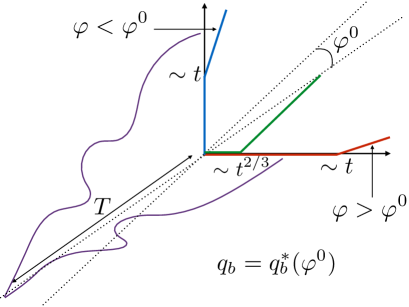
Refer to caption

Figure 9: Convergence to the stationary measure and equivalence between direction and stationarity parameter qbsubscript𝑞𝑏q_{b} in the Bernoulli-Geometric polymer. The optimal energies in the model with boundaries with parameter qbsubscript𝑞𝑏q_{b} are interpreted as differences of optimal energies for the point to point BG polymer (purple paths above) starting from infinity T1much-greater-than𝑇1T\gg 1 in the direction φ0superscript𝜑0\varphi^{0} such that qb=qb(φ0)subscript𝑞𝑏superscriptsubscript𝑞𝑏superscript𝜑0q_{b}=q_{b}^{*}(\varphi^{0}). Optimal path properties in the BG polymer with boundaries strongly depend on the observed direction. For φ>φ0𝜑superscript𝜑0\varphi>\varphi^{0} (resp. φ<φ0𝜑superscript𝜑0\varphi<\varphi^{0}) the optimal polymer path sticks to the vertical boundary (blue path) (resp. horizontal boundary (red path)) for a macroscopic amount of time tsimilar-toabsent𝑡\sim t. In the direction φ=φ0𝜑superscript𝜑0\varphi=\varphi^{0}, we conjecture following the work of Seppäläinen Seppalainen2012 that the optimal polymer path stays on the boundary for a time of order t2/3superscript𝑡23t^{2/3} only (green path).

Let us first comment on some elements that appeared in the proof of (VI.2.1) in Sec. VI.2. There we defined, for a fixed direction (s1,s2)=(1/2+φ,1/2φ)subscript𝑠1subscript𝑠212𝜑12𝜑(s_{1},s_{2})=(1/2+\varphi,1/2-\varphi) and varying the boundary parameter qbsubscript𝑞𝑏q_{b}, two functions r1φ(qb)superscriptsubscript𝑟1𝜑subscript𝑞𝑏r_{1}^{\varphi}(q_{b}) and r2φ(qb)superscriptsubscript𝑟2𝜑subscript𝑞𝑏r_{2}^{\varphi}(q_{b}) (here we emphasize the dependence on φ𝜑\varphi of these quantities by superscript). These two functions correspond to the average length divided by t𝑡t spend by the optimal polymer path on the horizontal (for r1φ(qb)superscriptsubscript𝑟1𝜑subscript𝑞𝑏r_{1}^{\varphi}(q_{b})) or vertical (for r2φ(qb)superscriptsubscript𝑟2𝜑subscript𝑞𝑏r_{2}^{\varphi}(q_{b})) boundary of 2superscript2\mathbb{N}^{2}. Hence for qb<qb(φ)subscript𝑞𝑏superscriptsubscript𝑞𝑏𝜑q_{b}<q_{b}^{*}(\varphi) we saw that the polymer spends on average a macroscopic amount of his time (r1φ(qb)tsimilar-toabsentsuperscriptsubscript𝑟1𝜑subscript𝑞𝑏𝑡\sim r_{1}^{\varphi}(q_{b})t) on the horizontal boundary, while for qb>qb(φ)subscript𝑞𝑏superscriptsubscript𝑞𝑏𝜑q_{b}>q_{b}^{*}(\varphi) the polymer spends on average a macroscopic amount of his time (r2φ(qb)tsimilar-toabsentsuperscriptsubscript𝑟2𝜑subscript𝑞𝑏𝑡\sim r_{2}^{\varphi}(q_{b})t) on the vertical boundary.

Conversely, fixing now qb=qb(φ0)subscript𝑞𝑏superscriptsubscript𝑞𝑏superscript𝜑0q_{b}=q_{b}^{*}(\varphi^{0}) for some φ0]1/2,1/2[\varphi^{0}\in]-1/2,1/2[, and varying φ𝜑\varphi, for φ>φ0𝜑superscript𝜑0\varphi>\varphi^{0} (resp. φ<φ0𝜑superscript𝜑0\varphi<\varphi^{0}), the optimal polymer path spends on average a macroscopic amount of time r~1φ0(φ)tsimilar-toabsentsuperscriptsubscript~𝑟1subscript𝜑0𝜑𝑡\sim\tilde{r}_{1}^{\varphi_{0}}(\varphi)t (resp. r~2φ0(φ)tsuperscriptsubscript~𝑟2subscript𝜑0𝜑𝑡\tilde{r}_{2}^{\varphi_{0}}(\varphi)t) on the horizontal (resp. vertical) boundary with r~1φ0(φ)=r1φ(qb=qb(φ0))superscriptsubscript~𝑟1subscript𝜑0𝜑superscriptsubscript𝑟1𝜑subscript𝑞𝑏superscriptsubscript𝑞𝑏superscript𝜑0\tilde{r}_{1}^{\varphi_{0}}(\varphi)=r_{1}^{\varphi}(q_{b}=q_{b}^{*}(\varphi^{0})) (resp. r~2φ0(φ)=r2φ(qb=qb(φ0))superscriptsubscript~𝑟2subscript𝜑0𝜑superscriptsubscript𝑟2𝜑subscript𝑞𝑏superscriptsubscript𝑞𝑏superscript𝜑0\tilde{r}_{2}^{\varphi_{0}}(\varphi)=r_{2}^{\varphi}(q_{b}=q_{b}^{*}(\varphi^{0}))). Hence, for φ>φ0𝜑subscript𝜑0\varphi>\varphi_{0} (resp. φ<φ0𝜑subscript𝜑0\varphi<\varphi_{0}), the optimal energy 𝖤^t(x=(1/2+φ)t)subscript^𝖤𝑡𝑥12𝜑𝑡\hat{\sf E}_{t}(x=(1/2+\varphi)t) contains a sum of order t𝑡t terms of iid distributed RVs of the 𝖴𝖴{\sf U} type (resp. of the 𝖵𝖵{\sf V} type) and one thus expects the fluctuations of 𝖤^t(x=(1/2+φ)t)subscript^𝖤𝑡𝑥12𝜑𝑡\hat{\sf E}_{t}(x=(1/2+\varphi)t) to scale as t𝑡\sqrt{t}. Thus, in any direction φφ0𝜑superscript𝜑0\varphi\neq\varphi^{0}, one does not observe fluctuations of order t1/3superscript𝑡13t^{1/3} as could have naively been expected from KPZ universality, the reason being that the polymer is then typically pinned by one of the two attractive boundaries for a macroscopic (i.e. of order t𝑡t) amount of time.

An important question is then to understand how the fluctuations of 𝖤^t(x=(1/2+φ)t)subscript^𝖤𝑡𝑥12𝜑𝑡\hat{\sf E}_{t}(x=(1/2+\varphi)t) scale with t𝑡t when φ=φ0𝜑superscript𝜑0\varphi=\varphi^{0}. In Seppalainen2012 Seppäläinen showed in the Log-Gamma polymer case that these fluctuations scale with the characteristic exponent t1/3superscript𝑡13t^{1/3} as expected from KPZ universality, and a typical polymer path then only spend a time of order t2/3superscript𝑡23t^{2/3} on one of the two boundaries. It is likely that the arguments presented in Seppalainen2012 could be adapted to our models. We will not prove it here and continue by assuming that the fluctuations of 𝖤^t(x=(1/2+φ)t)subscript^𝖤𝑡𝑥12𝜑𝑡\hat{\sf E}_{t}(x=(1/2+\varphi)t) are of order t1/3superscript𝑡13t^{1/3} when φ=φ0𝜑superscript𝜑0\varphi=\varphi^{0}.

Following the above remarks, it is clear that the direction φ=φ0𝜑superscript𝜑0\varphi=\varphi^{0} is a special direction for the model with boundaries. It is the only direction for which the fluctuations of the optimal energy scale with the expected t1/3superscript𝑡13t^{1/3} exponent. Moreover, the direction φ=φ0𝜑superscript𝜑0\varphi=\varphi^{0} is the only direction for which the mean optimal energy in the model with boundaries 𝖿^BGp.u.l.(φ0,qb(φ0))superscriptsubscript^𝖿BGformulae-sequencepulsuperscript𝜑0superscriptsubscript𝑞𝑏superscript𝜑0\hat{\sf f}_{{\rm BG}}^{{\rm p.u.l.}}(\varphi^{0},q_{b}^{*}(\varphi^{0})) coincide with the mean optimal energy of the underlying model without boundaries 𝖿BGp.u.l.(φ0)superscriptsubscript𝖿BGformulae-sequencepulsuperscript𝜑0{\sf f}_{{\rm BG}}^{{\rm p.u.l.}}(\varphi^{0}). From these two facts, it appears reasonable to conjecture that the equivalence in law (VI.29), which a-priori only holds for t,xTmuch-less-than𝑡𝑥𝑇t,x\ll T, also holds for t=O(T)𝑡𝑂𝑇t=O(T) with x=(1/2+φ0)t+x^𝑥12superscript𝜑0𝑡^𝑥x=(1/2+\varphi^{0})t+\hat{x} with x^=O(1)^𝑥𝑂1\hat{x}=O(1). That is, asymptotic properties of the model with boundaries with parameter qb=qb(φ0)subscript𝑞𝑏superscriptsubscript𝑞𝑏superscript𝜑0q_{b}=q_{b}^{*}(\varphi^{0}) reproduce those of the model without boundaries if one looks in the characteristic direction φ=φ0𝜑superscript𝜑0\varphi=\varphi^{0}.

On the other hand for directions φφ0𝜑superscript𝜑0\varphi\neq\varphi^{0} it is clear that asymptotic properties of the model with boundaries cannot be interpreted in the model without boundaries and the equivalence in law (VI.29) does not hold anymore. An example of such properties is as follows. In a direction φ>φ0𝜑superscript𝜑0\varphi>\varphi^{0} we have

𝖤^t((1/2+φ)t)subscript^𝖤𝑡12𝜑𝑡\displaystyle\hat{\sf E}_{t}((1/2+\varphi)t) =𝖤^t((1/2+φ)t)𝖤^t((1/2+φ0)t)+𝖤^t((1/2+φ0)t)absentsubscript^𝖤𝑡12𝜑𝑡subscript^𝖤𝑡12superscript𝜑0𝑡subscript^𝖤𝑡12superscript𝜑0𝑡\displaystyle=\hat{\sf E}_{t}((1/2+\varphi)t)-\hat{\sf E}_{t}((1/2+\varphi^{0})t)+\hat{\sf E}_{t}((1/2+\varphi^{0})t) (VI.30)
=x=(1/2+φ0)tx=(1/2+φ)t(𝖴^t(x)𝖵^t(x))+𝖤^t((1/2+φ0)t).absentsuperscriptsubscript𝑥12superscript𝜑0𝑡𝑥12𝜑𝑡subscript^𝖴𝑡𝑥subscript^𝖵𝑡𝑥subscript^𝖤𝑡12superscript𝜑0𝑡\displaystyle=\sum_{x=(1/2+\varphi^{0})t}^{x=(1/2+\varphi)t}\left(\hat{\sf U}_{t}(x)-\hat{\sf V}_{t}(x)\right)+\hat{\sf E}_{t}((1/2+\varphi^{0})t)\ .

Subtracting the average values over disorder in the above equation, one gets that 𝖤^t((1/2+φ)t)t𝖿^BGp.u.l.(φ,qb)subscript^𝖤𝑡12𝜑𝑡𝑡subscriptsuperscript^𝖿formulae-sequencepulBG𝜑subscript𝑞𝑏\hat{\sf E}_{t}((1/2+\varphi)t)-t\hat{\sf f}^{{\rm p.u.l.}}_{{\rm BG}}(\varphi,q_{b}) is the sum of t(φφ0)𝑡𝜑superscript𝜑0t(\varphi-\varphi^{0}) independent centered RVs (note that these RVs indeed live on a down-right path πdr(t)superscriptsubscript𝜋𝑑𝑟𝑡\pi_{dr}^{(t)}) distributed as 𝖴𝖵𝖴¯+𝖵¯𝖴𝖵¯𝖴¯𝖵{\sf U}-{\sf V}-\overline{{\sf U}}+\overline{{\sf V}}, and of another centered term 𝖤^t((1/2+φ0)t)t𝖿^BGp.u.l.(φ0,qb)subscript^𝖤𝑡12superscript𝜑0𝑡𝑡subscriptsuperscript^𝖿formulae-sequencepulBGsuperscript𝜑0subscript𝑞𝑏\hat{\sf E}_{t}((1/2+\varphi^{0})t)-t\hat{\sf f}^{{\rm p.u.l.}}_{{\rm BG}}(\varphi^{0},q_{b}) whose fluctuations scale as t1/3superscript𝑡13t^{1/3} (admitting the above discussion). Hence it is then clear that in the large time limit the fluctuations of 𝖤^t((1/2+φ)t)subscript^𝖤𝑡12𝜑𝑡\hat{\sf E}_{t}((1/2+\varphi)t) are Gaussian distributed and we have the convergence in law

𝖤^t((1/2+φ)t)t𝖿^BGp.u.l.(φ,qb)σ(φ)ttχ𝒩(0,1),subscriptsimilar-to𝑡subscript^𝖤𝑡12𝜑𝑡𝑡subscriptsuperscript^𝖿formulae-sequencepulBG𝜑subscript𝑞𝑏𝜎𝜑𝑡subscript𝜒𝒩01\displaystyle\frac{\hat{\sf E}_{t}((1/2+\varphi)t)-t\hat{\sf f}^{{\rm p.u.l.}}_{{\rm BG}}(\varphi,q_{b})}{\sigma(\varphi)\sqrt{t}}\sim_{t\to\infty}\chi_{{\cal N}(0,1)}\ , (VI.31)

where here, qb=qb(φ0)subscript𝑞𝑏superscriptsubscript𝑞𝑏superscript𝜑0q_{b}=q_{b}^{*}(\varphi^{0}), σ(φ)=(φφ0)(𝖴2¯c+𝖵2¯c)𝜎𝜑𝜑superscript𝜑0superscript¯superscript𝖴2𝑐superscript¯superscript𝖵2𝑐\sigma(\varphi)=\sqrt{(\varphi-\varphi^{0})\left(\overline{{\sf U}^{2}}^{c}+\overline{{\sf V}^{2}}^{c}\right)} and χ(0,1)𝒩\chi{{}_{\cal N}(0,1)} is a RV distributed with a standard unit centered normal distribution.

VII Numerical results for the zero-temperature model

In this section we report results of numerical simulations of the point to point Bernoulli-Geometric polymer (without boundaries, see Def. III.4) for three sets of parameters. For each set we have q=0.5𝑞0.5q=0.5 and we vary the anisotropy parameter: we consider an almost isotropic case q1=0.1subscriptsuperscript𝑞10.1q^{\prime}_{1}=0.1 and two strongly anisotropic cases q2=0.8subscriptsuperscript𝑞20.8q^{\prime}_{2}=0.8 and q3=0.9subscriptsuperscript𝑞30.9q^{\prime}_{3}=0.9. For each set we perform 2×1052superscript1052\times 10^{5} simulations of independent random environments of size 2048×2048204820482048\times 2048. For each random environment we measure using a transfer matrix algorithm the optimal energy and horizontal and vertical energy differences 𝖤tj((1/2+φk)tj)subscript𝖤subscript𝑡𝑗12subscript𝜑𝑘subscript𝑡𝑗{\sf E}_{t_{j}}((1/2+\varphi_{k})t_{j}), 𝖴tj((1/2+φk)tj):=𝖤tj((1/2+φk)tj)𝖤tj1((1/2+φk)tj1)assignsubscript𝖴subscript𝑡𝑗12subscript𝜑𝑘subscript𝑡𝑗subscript𝖤subscript𝑡𝑗12subscript𝜑𝑘subscript𝑡𝑗subscript𝖤subscript𝑡𝑗112subscript𝜑𝑘subscript𝑡𝑗1{\sf U}_{t_{j}}((1/2+\varphi_{k})t_{j}):={\sf E}_{t_{j}}((1/2+\varphi_{k})t_{j})-{\sf E}_{t_{j}-1}((1/2+\varphi_{k})t_{j}-1) and 𝖵tj((1/2+φk)tj):=𝖤tj((1/2+φk)tj)𝖤tj1((1/2+φk)tj)assignsubscript𝖵subscript𝑡𝑗12subscript𝜑𝑘subscript𝑡𝑗subscript𝖤subscript𝑡𝑗12subscript𝜑𝑘subscript𝑡𝑗subscript𝖤subscript𝑡𝑗112subscript𝜑𝑘subscript𝑡𝑗{\sf V}_{t_{j}}((1/2+\varphi_{k})t_{j}):={\sf E}_{t_{j}}((1/2+\varphi_{k})t_{j})-{\sf E}_{t_{j}-1}((1/2+\varphi_{k})t_{j}) for different times tj=2j+5subscript𝑡𝑗superscript2𝑗5t_{j}=2^{j+5} with j=1,,6𝑗16j=1,\dots,6 (hence t1=64subscript𝑡164t_{1}=64 and t6=2048subscript𝑡62048t_{6}=2048) and different angle parameters φk=0.4+k110subscript𝜑𝑘0.4𝑘110\varphi_{k}=-0.4+\frac{k-1}{10} with k=1,,9𝑘19k=1,\dots,9.

We first compare in Fig.10 for each set of parameters our exact result for the asymptotic value of the mean optimal energy per-unit-length (VI.17) with the numerically obtained value 𝖤tj((1/2+φk)tj)¯/tj¯subscript𝖤subscript𝑡𝑗12subscript𝜑𝑘subscript𝑡𝑗subscript𝑡𝑗\overline{{\sf E}_{t_{j}}((1/2+\varphi_{k})t_{j})}/t_{j} for j=6𝑗6j=6 (i.e. polymers of length t=t6=2048𝑡subscript𝑡62048t=t_{6}=2048 for each set of parameters and each angle φksubscript𝜑𝑘\varphi_{k}. We obtain an excellent agreement.

Refer to caption

Figure 10: Comparison between the exact result for the mean asymptotic optimal energy per-unit-length in the Bernoulli-Geometric polymer 𝖿BGp.u.l.(φ)superscriptsubscript𝖿BGformulae-sequencepul𝜑{\sf f}_{{\rm BG}}^{{\rm p.u.l.}}(\varphi) (see (VI.17)) for q=0.5𝑞0.5q=0.5 and q=q1=0.1superscript𝑞subscript𝑞10.1q^{\prime}=q_{1}=0.1 (blue line), q=q2=0.8superscript𝑞subscript𝑞20.8q^{\prime}=q_{2}=0.8 (orange line) and q=q3=0.9superscript𝑞subscript𝑞30.9q^{\prime}=q_{3}=0.9 (green line) and the numerically obtained value 𝖤t6((1/2+φk)t6)¯/t6¯subscript𝖤subscript𝑡612subscript𝜑𝑘subscript𝑡6subscript𝑡6\overline{{\sf E}_{t_{6}}((1/2+\varphi_{k})t_{6})}/t_{6} for each set of parameters and each angle φksubscript𝜑𝑘\varphi_{k} (dots, same color code).

We then check our conjecture (III.45). The latter notably implies, combined with Prop. III.1, that the differences of horizontal and vertical energies in a given direction, 𝖴tj((1/2+φk)tj)subscript𝖴subscript𝑡𝑗12subscript𝜑𝑘subscript𝑡𝑗{\sf U}_{t_{j}}((1/2+\varphi_{k})t_{j}) and 𝖵tj((1/2+φk)tj)subscript𝖵subscript𝑡𝑗12subscript𝜑𝑘subscript𝑡𝑗{\sf V}_{t_{j}}((1/2+\varphi_{k})t_{j}), converge to independent random variables distributed as 𝖴𝖴{\sf U} and 𝖵𝖵{\sf V} in (III.5), with for each φksubscript𝜑𝑘\varphi_{k} the boundary parameter qbsubscript𝑞𝑏q_{b} chosen as qb=qb(φk)subscript𝑞𝑏superscriptsubscript𝑞𝑏subscript𝜑𝑘q_{b}=q_{b}^{*}(\varphi_{k}), the solution of the saddle-point equation (III.41) with (s1,s2)=(1/2φk,1/2+φk)subscript𝑠1subscript𝑠212subscript𝜑𝑘12subscript𝜑𝑘(s_{1},s_{2})=(1/2-\varphi_{k},1/2+\varphi_{k}). In Fig.11 we analyze the numerical results for the set of parameters with q=q3=0.9superscript𝑞subscriptsuperscript𝑞30.9q^{\prime}=q^{\prime}_{3}=0.9. We first obtain numerically the PDF of horizontal and vertical differences of optimal energies 𝖴t6((1/2+φ8)t6)subscript𝖴subscript𝑡612subscript𝜑8subscript𝑡6{\sf U}_{t_{6}}((1/2+\varphi_{8})t_{6}), 𝖵t6((1/2+φ8)t6)subscript𝖵subscript𝑡612subscript𝜑8subscript𝑡6{\sf V}_{t_{6}}((1/2+\varphi_{8})t_{6}) for an angle φ=φ8=0.3𝜑subscript𝜑80.3\varphi=\varphi_{8}=0.3 and polymers of length t=t6=2048𝑡subscript𝑡62048t=t_{6}=2048, and compare it with our asymptotic prediction (III.5) (the appropriate boundary parameter is there found to be qb0.922824similar-to-or-equalssuperscriptsubscript𝑞𝑏0.922824q_{b}^{*}\simeq 0.922824). We obtain an excellent agreement. To check the independence of the RVs, we estimate numerically the normalized covariance 𝖴tj((1/2+φ8)tj)𝖵tj((1/2+φ8)tj)¯c𝖴tj((1/2+φ8)tj)¯×𝖵tj((1/2+φ8)tj)¯superscript¯subscript𝖴subscript𝑡𝑗12subscript𝜑8subscript𝑡𝑗subscript𝖵subscript𝑡𝑗12subscript𝜑8subscript𝑡𝑗𝑐¯subscript𝖴subscript𝑡𝑗12subscript𝜑8subscript𝑡𝑗¯subscript𝖵subscript𝑡𝑗12subscript𝜑8subscript𝑡𝑗\frac{\overline{{\sf U}_{t_{j}}((1/2+\varphi_{8})t_{j}){\sf V}_{t_{j}}((1/2+\varphi_{8})t_{j})}^{c}}{\overline{{\sf U}_{t_{j}}((1/2+\varphi_{8})t_{j})}\times\overline{{\sf V}_{t_{j}}((1/2+\varphi_{8})t_{j})}} and study its behavior as a function of t𝑡t. Although fluctuations are large, the normalized covariance clearly decays to 00 with increasing t𝑡t, a signature of the independence of the RVs. In Fig.12 we report similarly satisfying results for the set of parameters with q=0.8superscript𝑞0.8q^{\prime}=0.8 and in the direction φ=φ2=0.3𝜑subscript𝜑20.3\varphi=\varphi_{2}=-0.3 (there the appropriate boundary parameter is found to be qb0.667665similar-to-or-equalssuperscriptsubscript𝑞𝑏0.667665q_{b}^{*}\simeq 0.667665).

Refer to caption Refer to caption Refer to caption

Figure 11: Left: (resp. Middle:) Comparison between the numerically obtained PDF of 𝖴t6((1/2+φ8)t6)subscript𝖴subscript𝑡612subscript𝜑8subscript𝑡6{\sf U}_{t_{6}}((1/2+\varphi_{8})t_{6}) (resp. 𝖵t6((1/2+φ8)t6)subscript𝖵subscript𝑡612subscript𝜑8subscript𝑡6{\sf V}_{t_{6}}((1/2+\varphi_{8})t_{6})) in the simulations with parameters q=0.5𝑞0.5q=0.5, q=0.9superscript𝑞0.9q^{\prime}=0.9 (yellow histogram) and the PDF of 𝖴𝖴{\sf U} (resp. 𝖵𝖵{\sf V}) given in (III.5) with qb=qb0.922824subscript𝑞𝑏superscriptsubscript𝑞𝑏similar-to-or-equals0.922824q_{b}=q_{b}^{*}\simeq 0.922824 (blue dots). Right: numerically obtained normalized covariance 𝖴tj((1/2+φ8)tj)𝖵tj((1/2+φ8)tj)¯c𝖴tj((1/2+φ8)tj)¯×𝖵tj((1/2+φ8)tj)¯superscript¯subscript𝖴subscript𝑡𝑗12subscript𝜑8subscript𝑡𝑗subscript𝖵subscript𝑡𝑗12subscript𝜑8subscript𝑡𝑗𝑐¯subscript𝖴subscript𝑡𝑗12subscript𝜑8subscript𝑡𝑗¯subscript𝖵subscript𝑡𝑗12subscript𝜑8subscript𝑡𝑗\frac{\overline{{\sf U}_{t_{j}}((1/2+\varphi_{8})t_{j}){\sf V}_{t_{j}}((1/2+\varphi_{8})t_{j})}^{c}}{\overline{{\sf U}_{t_{j}}((1/2+\varphi_{8})t_{j})}\times\overline{{\sf V}_{t_{j}}((1/2+\varphi_{8})t_{j})}} in the simulations with parameters q=0.5𝑞0.5q=0.5, q=0.9superscript𝑞0.9q^{\prime}=0.9 as a function of tjsubscript𝑡𝑗t_{j} (blue dots). Error bars are 3limit-from33-sigma Gaussian estimates.

Refer to caption Refer to caption Refer to caption

Figure 12: Left: (resp. Middle:) Comparison between the numerically obtained PDF of 𝖴t6((1/2+φ2)t6)subscript𝖴subscript𝑡612subscript𝜑2subscript𝑡6{\sf U}_{t_{6}}((1/2+\varphi_{2})t_{6}) (resp. 𝖵t6((1/2+φ2)t6)subscript𝖵subscript𝑡612subscript𝜑2subscript𝑡6{\sf V}_{t_{6}}((1/2+\varphi_{2})t_{6})) in the simulations with parameters q=0.5𝑞0.5q=0.5, q=0.8superscript𝑞0.8q^{\prime}=0.8 (yellow histogram) and the PDF of 𝖴𝖴{\sf U} (resp. 𝖵𝖵{\sf V}) given in (III.5) with qb=qb0.667665subscript𝑞𝑏superscriptsubscript𝑞𝑏similar-to-or-equals0.667665q_{b}=q_{b}^{*}\simeq 0.667665 (blue dots). Right: numerically obtained normalized covariance 𝖴tj((1/2+φ2)tj)𝖵tj((1/2+φ2)tj)¯c𝖴tj((1/2+φ2)tj)¯×𝖵tj((1/2+φ2)tj)¯superscript¯subscript𝖴subscript𝑡𝑗12subscript𝜑2subscript𝑡𝑗subscript𝖵subscript𝑡𝑗12subscript𝜑2subscript𝑡𝑗𝑐¯subscript𝖴subscript𝑡𝑗12subscript𝜑2subscript𝑡𝑗¯subscript𝖵subscript𝑡𝑗12subscript𝜑2subscript𝑡𝑗\frac{\overline{{\sf U}_{t_{j}}((1/2+\varphi_{2})t_{j}){\sf V}_{t_{j}}((1/2+\varphi_{2})t_{j})}^{c}}{\overline{{\sf U}_{t_{j}}((1/2+\varphi_{2})t_{j})}\times\overline{{\sf V}_{t_{j}}((1/2+\varphi_{2})t_{j})}} in the simulations with parameters q=0.5𝑞0.5q=0.5, q=0.8superscript𝑞0.8q^{\prime}=0.8 as a function of tjsubscript𝑡𝑗t_{j} (blue dots). Error bars are 3limit-from33-sigma Gaussian estimates.

VIII Conclusion

In this paper we have obtained the stationary measure of the Inverse-Beta polymer, an exactly solvable, anisotropic finite temperature model of DP on the square lattice recently introduced in usIBeta . As we discussed, the stationary model can be either studied on 2superscript2\mathbb{Z}^{2} with a random initial condition for the polymer such that the free-energy of the DP performs a random walk with inverse-beta distributed increments, or also conveniently in a model on the upper-right quadrant 2superscript2\mathbb{N}^{2} with special boundary conditions. This thus confers to the IB polymer a second exact solvability property that complements the coordinate Bethe ansatz solvability shown in usIBeta .

In parallel we introduced a new model of zero temperature DP on the square lattice, the Bernoulli-Geometric polymer. It is obtained by appropriately discretizing the distributions of random energies of the zero temperature limit of the Inverse-Beta polymer from Bernoulli-Exponential distributions to Bernoulli-Geometric distributions. This model is thus canonically dual to the IB polymer. In two different limits the model becomes either a first passage percolation problem, or a last passage percolation problem. We showed that its stationary measure could be exactly obtained, thus conferring to this new model at least one exact solvability property.

We also showed that the two stationary measures are reversible and satisfy detailed balance. We obtained the mean quenched free-energy (resp. optimal energy) in the IB (resp. BG) polymer. For the IB polymer, the obtained result (III.38) coincides with a previously obtained result of usIBeta , therefore confirming the validity of the non-rigorous approach of usIBeta , while in the BG polymer case, (III.40) is genuinely new. In both cases, these results allowed us to discuss the convergence of each model to their stationary measure. Finally in Sec. VII we reported the results of numerical simulations of the BG polymer and compared them with a very good agreement to our results.

Many possible research directions remain for the future. One interesting direction would be to understand if the models studied in this paper possess other exact solvability properties. Indeed for both models it is not clear whether or not combinatorial mappings similar to RSK and gRSK correspondences could be developed, although they both interpolate between models for which these correspondences can be applied (gRSK at finite temperature logsep2 ; StrictWeak2 and RSK at 00 temperature Johansson2000 ; OConnell2005 ). The question of the Bethe ansatz solvability of these models is also interesting. For the IB polymer it was shown in usIBeta that the moment problem is exactly solvable by coordinate BA but another BA solvability could exist. Indeed in the Log-Gamma case it was shown in usLogGamma that the moment problem was BA solvable, but is is also known that the partition sum of the Log-Gamma polymer can be interpreted PetrovMatveev2015 as an observable of a BA solvable interacting particles system on \mathbb{Z}, the q-Push TASEP PetrovBorodin2013 ; PetrovCorwin2015 . The same is true for the Strict-Weak polymer which can be mapped onto an observable of the q-TASEP StrictWeak1 . Exhibiting a similar mapping for the IB polymer case remains an open question. For the BG polymer introduced in this paper the question of BA solvability is also open. We note that in the isotropic limit of the model, i.e. last passage percolation with geometric weights, the optimal energy can be interpreted as waiting times of the TASEP with geometric waiting times and step initial condition, which can be solved by BA. Furthermore, we note that a version of the q-TASEP with Bernoulli and Geometric waiting times was already considered in BorodinCorwinDiscretTimeQ where the authors notably proved BA solvability. Although it is not clear how to map the optimal energies in the BG polymer to the waiting times of an interacting particles system (since the random energies can be both positive and negative), this could be an interesting approach.

Another interesting direction of research would be to understand how to obtain more systematically models of directed polymers with exact solvability properties and how to classify them. For the case of Bethe ansatz solvability of the moment problem for models of DPs at finite temperature, this was already mostly accomplished in usIBeta . The question remains open for BA solvability of models at zero temperature and for other type of exact solvability properties such as the possibility of writing down the stationary measure exactly. If this was accomplished it would be interesting to see whether or not the two classes coincide. We note that in the related context of zero-range-processes (ZRP) with simultaneous updates, it was recently shown that all BA solvable models have factorizable steady-states, but the converse is not true povolotsky2013integrability . For the DP case, a step in this direction was already made since in Seppalainen2012 it was shown that the Log-Gamma was the unique model at finite temperature with on site disorder for which it is possible to write down exactly the SM, and the Log-Gamma also appeared as the unique finite temperature model with on site disorder exactly solvable by BA in the classification of usIBeta . More generally it would be interesting to gain a better understanding of the links between different exact solvability properties.

Acknowledgements.
This paper would have never existed without the numerous discussions I had with Timo Seppäläinen, discussions during which he kindly took the time to explain to me the techniques and results developed and obtained by him and his coworkers for the Log-Gamma polymer. These were a great source of inspiration for this work. He also took an active part during the first stages of research on the stationary measure of the Inverse-Beta polymer and shared with me related new results on the Beta polymer SeppalainenInprep . I warmly thank him for that. I am also grateful to Guillaume Barraquand for many discussions and remarks on the existing mathematical literature, as well as to Francis Comets, Ivan Corwin, Thomas Gueudré, Vivien Lecomte, Jeremy Quastel and Leonid Petrov for interesting discussions. Last but not least, I would like to warmly thank Pierre Le Doussal who introduced me and taught me most of the things I know on this topic through multiple discussions and collaborations on related subjects. I also thank him for useful comments on a first version of this manuscript. I acknowledge the KITP in Santa Barbara for hospitality during the first stages of redaction of this work. This research was supported in part by the National Science Foundation under Grant No. NSF PHY11-25915.

Appendix A Proof of the properties of the finite temperature reversibility-stationarity map

In this appendix we prove Prop. IV.1, Prop. IV.2 being trivial. We thus consider three independent random variables (U,V,W)𝑈𝑉𝑊(U,V,W) distributed as in (III.2) and (III.3) and consider the RVs (U,V,W)=ϕ(U,V,W)superscript𝑈superscript𝑉superscript𝑊italic-ϕ𝑈𝑉𝑊(U^{\prime},V^{\prime},W^{\prime})=\phi(U,V,W) as given in (IV.3). The Jacobian of the transformation (U,V,W)(U,V,W)𝑈𝑉𝑊superscript𝑈superscript𝑉superscript𝑊(U,V,W)\to(U^{\prime},V^{\prime},W^{\prime}) is easily computed as, schematically,

det(ϕ(U,V,W)(U,V,W))=UW+U+VWUV<0.detitalic-ϕ𝑈𝑉𝑊𝑈𝑉𝑊𝑈𝑊𝑈𝑉𝑊𝑈𝑉0\displaystyle{\rm det}\left(\frac{\partial\phi(U,V,W)}{\partial(U,V,W)}\right)=-\frac{UW+U+VW}{UV}<0\ . (A.1)

The PDF of the triplet (U,V,W)superscript𝑈superscript𝑉superscript𝑊(U^{\prime},V^{\prime},W^{\prime}) is then directly evaluated as

P(U,V,W)=PU(ϕ(1)(U,V,W))PV(ϕ(1)(U,V,W))PW(ϕ(1)(U,V,W))×UVUW+U+VW .𝑃superscript𝑈superscript𝑉superscript𝑊subscript𝑃𝑈superscriptitalic-ϕ1superscript𝑈superscript𝑉superscript𝑊subscript𝑃𝑉superscriptitalic-ϕ1superscript𝑈superscript𝑉superscript𝑊subscript𝑃𝑊superscriptitalic-ϕ1superscript𝑈superscript𝑉superscript𝑊𝑈𝑉𝑈𝑊𝑈𝑉𝑊 \displaystyle P(U^{\prime},V^{\prime},W^{\prime})=P_{U}(\phi^{(1)}(U^{\prime},V^{\prime},W^{\prime}))P_{V}(\phi^{(1)}(U^{\prime},V^{\prime},W^{\prime}))P_{W}(\phi^{(1)}(U^{\prime},V^{\prime},W^{\prime}))\times\frac{UV}{UW+U+VW}\  . (A.2)

Where we introduced the PDF of the independent RVs (U,V,W)𝑈𝑉𝑊(U,V,W) as noted in (III.2) and (III.3) and used the fact that ϕitalic-ϕ\phi is an involution. It is then directly checked that

P(U,V,W)=PU(U)PV(V)PW(W) ,𝑃superscript𝑈superscript𝑉superscript𝑊subscript𝑃𝑈superscript𝑈subscript𝑃𝑉superscript𝑉subscript𝑃𝑊superscript𝑊 \displaystyle P(U^{\prime},V^{\prime},W^{\prime})=P_{U}(U^{\prime})P_{V}(V^{\prime})P_{W}(W^{\prime})\  , (A.3)

hence showing that Usuperscript𝑈U^{\prime}, Vsuperscript𝑉V^{\prime} and Wsuperscript𝑊W^{\prime} are independent and distributed as UUsimilar-tosuperscript𝑈𝑈U^{\prime}\sim U, VVsimilar-tosuperscript𝑉𝑉V^{\prime}\sim V and WWsimilar-tosuperscript𝑊𝑊W^{\prime}\sim W.

Appendix B Proof of the properties of the zero temperature stationarity map

In this Appendix we prove Prop. V.1 and Prop. V.2. Let us first prove the detailed balance property Prop. V.2b. We thus consider 𝖴𝖵(𝗎,𝗏)perpendicular-to𝖴𝖵perpendicular-to𝗎𝗏{\sf U}\perp{\sf V}\perp({\sf u},{\sf v}) distributed as in (III.4) and (III.5). Let us first compute the conditional probability

Ψ(k𝖴,k𝖵,k𝖴,k𝖵):=Proba(((𝖴,𝖵)=(k𝖴,k𝖵)|(𝖴,𝖵)=(k𝖴,k𝖵))\displaystyle\Psi(k_{{\sf U}^{\prime}},k_{{\sf V}^{\prime}},k_{{\sf U}},k_{{\sf V}}):=Proba\left((({\sf U}^{\prime},{\sf V}^{\prime})=(k_{{\sf U}^{\prime}},k_{{\sf V}^{\prime}})|({\sf U},{\sf V})=(k_{{\sf U}},k_{{\sf V}})\right) (B.1)

where k𝖴subscript𝑘𝖴k_{{\sf U}}\in\mathbb{N}, k𝖵subscript𝑘𝖵subscriptk_{{\sf V}}\in{\mathbb{Z}}_{-}, 𝖴=min(𝗎,𝗏+𝖴𝖵)superscript𝖴min𝗎𝗏𝖴𝖵{\sf U}^{\prime}={\rm min}\left({\sf u},{\sf v}+{\sf U}-{\sf V}\right) and 𝖵=min(𝗎+𝖵𝖴,𝗏)=𝖴+𝖵𝖴superscript𝖵min𝗎𝖵𝖴𝗏superscript𝖴𝖵𝖴{\sf V}^{\prime}={\rm min}\left({\sf u}+{\sf V}-{\sf U},{\sf v}\right)={\sf U}^{\prime}+{\sf V}-{\sf U}. We have

Ψ(k𝖴,k𝖵,k𝖴,k𝖵)=Ψsubscript𝑘superscript𝖴subscript𝑘superscript𝖵subscript𝑘𝖴subscript𝑘𝖵absent\displaystyle\Psi(k_{{\sf U}^{\prime}},k_{{\sf V}^{\prime}},k_{{\sf U}},k_{{\sf V}})= p𝗎𝗏Gq=0(1q)(q)Gqδ(k𝖴=min(Gq,Gq+k𝖴k𝖵))δ(k𝖵=k𝖴+k𝖵k𝖴)UNKNOWNsubscript𝑝𝗎𝗏superscriptsubscriptsubscript𝐺𝑞01𝑞superscript𝑞subscript𝐺𝑞𝛿subscript𝑘superscript𝖴minsubscript𝐺𝑞subscript𝐺𝑞subscript𝑘𝖴subscript𝑘𝖵𝛿subscript𝑘superscript𝖵subscript𝑘superscript𝖴subscript𝑘𝖵subscript𝑘𝖴UNKNOWN\displaystyle p_{{\sf u}{\sf v}}\sum_{G_{q}=0}^{\infty}(1-q)(q)^{G_{q}}\delta(k_{{\sf U}^{\prime}}={\rm min}\left(-G_{q},-G_{q}+k_{{\sf U}}-k_{{\sf V}}\right))\delta(k_{{\sf V}^{\prime}}=k_{{\sf U}^{\prime}}+k_{{\sf V}}-k_{{\sf U}}) 
+(1p𝗎𝗏)Gq=0(1q)(q)Gqδ(k𝖴=min(1+Gq,k𝖴k𝖵))δ(k𝖵=k𝖴+k𝖵k𝖴)1subscript𝑝𝗎𝗏superscriptsubscriptsuperscriptsubscript𝐺𝑞01superscript𝑞superscriptsuperscript𝑞superscriptsubscript𝐺𝑞𝛿subscript𝑘superscript𝖴min1superscriptsubscript𝐺𝑞subscript𝑘𝖴subscript𝑘𝖵𝛿subscript𝑘superscript𝖵subscript𝑘superscript𝖴subscript𝑘𝖵subscript𝑘𝖴\displaystyle+(1-p_{{\sf u}{\sf v}})\sum_{G_{q}^{\prime}=0}^{\infty}(1-q^{\prime})(q^{\prime})^{G_{q}^{\prime}}\delta(k_{{\sf U}^{\prime}}={\rm min}\left(1+G_{q}^{\prime},k_{{\sf U}}-k_{{\sf V}}\right))\delta(k_{{\sf V}^{\prime}}=k_{{\sf U}^{\prime}}+k_{{\sf V}}-k_{{\sf U}})
p𝗎𝗏Gq=0(1q)(q)Gqδ(k𝖴=Gq)δ(k𝖴>k𝖵)δ(k𝖵=k𝖴+k𝖵k𝖴)subscript𝑝𝗎𝗏superscriptsubscriptsubscript𝐺𝑞01𝑞superscript𝑞subscript𝐺𝑞𝛿subscript𝑘superscript𝖴subscript𝐺𝑞𝛿subscript𝑘𝖴subscript𝑘𝖵𝛿subscript𝑘superscript𝖵subscript𝑘superscript𝖴subscript𝑘𝖵subscript𝑘𝖴\displaystyle p_{{\sf u}{\sf v}}\sum_{G_{q}=0}^{\infty}(1-q)(q)^{G_{q}}\delta(k_{{\sf U}^{\prime}}=-G_{q})\delta(k_{{\sf U}}>k_{{\sf V}})\delta(k_{{\sf V}^{\prime}}=k_{{\sf U}^{\prime}}+k_{{\sf V}}-k_{{\sf U}})
+p𝗎𝗏Gq=0(1q)(q)Gqδ(k𝖴=Gq+k𝖴k𝖵)δ(k𝖴k𝖵)δ(k𝖵=k𝖴+k𝖵k𝖴)subscript𝑝𝗎𝗏superscriptsubscriptsubscript𝐺𝑞01𝑞superscript𝑞subscript𝐺𝑞𝛿subscript𝑘superscript𝖴subscript𝐺𝑞subscript𝑘𝖴subscript𝑘𝖵𝛿subscript𝑘𝖴subscript𝑘𝖵𝛿subscript𝑘superscript𝖵subscript𝑘superscript𝖴subscript𝑘𝖵subscript𝑘𝖴\displaystyle+p_{{\sf u}{\sf v}}\sum_{G_{q}=0}^{\infty}(1-q)(q)^{G_{q}}\delta(k_{{\sf U}^{\prime}}=-G_{q}+k_{{\sf U}}-k_{{\sf V}})\delta(k_{{\sf U}}\leq k_{{\sf V}})\delta(k_{{\sf V}^{\prime}}=k_{{\sf U}^{\prime}}+k_{{\sf V}}-k_{{\sf U}})
+(1p𝗎𝗏)Gq=0(1q)(q)Gqδ(k𝖴=1+Gq)δ(k𝖴k𝖵>1+Gq)δ(k𝖵=k𝖴+k𝖵k𝖴)1subscript𝑝𝗎𝗏superscriptsubscriptsuperscriptsubscript𝐺𝑞01superscript𝑞superscriptsuperscript𝑞superscriptsubscript𝐺𝑞𝛿subscript𝑘superscript𝖴1superscriptsubscript𝐺𝑞𝛿subscript𝑘𝖴subscript𝑘𝖵1superscriptsubscript𝐺𝑞𝛿subscript𝑘superscript𝖵subscript𝑘superscript𝖴subscript𝑘𝖵subscript𝑘𝖴\displaystyle+(1-p_{{\sf u}{\sf v}})\sum_{G_{q}^{\prime}=0}^{\infty}(1-q^{\prime})(q^{\prime})^{G_{q}^{\prime}}\delta(k_{{\sf U}^{\prime}}=1+G_{q}^{\prime})\delta(k_{{\sf U}}-k_{{\sf V}}>1+G_{q}^{\prime})\delta(k_{{\sf V}^{\prime}}=k_{{\sf U}^{\prime}}+k_{{\sf V}}-k_{{\sf U}})
+(1p𝗎𝗏)Gq=0(1q)(q)Gqδ(k𝖴=k𝖴k𝖵)δ(k𝖴k𝖵1+Gq)δ(k𝖵=k𝖴+k𝖵k𝖴),1subscript𝑝𝗎𝗏superscriptsubscriptsuperscriptsubscript𝐺𝑞01superscript𝑞superscriptsuperscript𝑞superscriptsubscript𝐺𝑞𝛿subscript𝑘superscript𝖴subscript𝑘𝖴subscript𝑘𝖵𝛿subscript𝑘𝖴subscript𝑘𝖵1superscriptsubscript𝐺𝑞𝛿subscript𝑘superscript𝖵subscript𝑘superscript𝖴subscript𝑘𝖵subscript𝑘𝖴\displaystyle+(1-p_{{\sf u}{\sf v}})\sum_{G_{q}^{\prime}=0}^{\infty}(1-q^{\prime})(q^{\prime})^{G_{q}^{\prime}}\delta(k_{{\sf U}^{\prime}}=k_{{\sf U}}-k_{{\sf V}})\delta(k_{{\sf U}}-k_{{\sf V}}\leq 1+G_{q}^{\prime})\delta(k_{{\sf V}^{\prime}}=k_{{\sf U}^{\prime}}+k_{{\sf V}}-k_{{\sf U}})\ ,

i.e.

Ψ(k𝖴,k𝖵,k𝖴,k𝖵)=Ψsubscript𝑘superscript𝖴subscript𝑘superscript𝖵subscript𝑘𝖴subscript𝑘𝖵absent\displaystyle\Psi(k_{{\sf U}^{\prime}},k_{{\sf V}^{\prime}},k_{{\sf U}},k_{{\sf V}})= p𝗎𝗏(1q)(q)k𝖴δ(k𝖴0)δ(k𝖴>k𝖵)δ(k𝖵=k𝖴+k𝖵k𝖴)subscript𝑝𝗎𝗏1𝑞superscript𝑞subscript𝑘superscript𝖴𝛿subscript𝑘superscript𝖴0𝛿subscript𝑘𝖴subscript𝑘𝖵𝛿subscript𝑘superscript𝖵subscript𝑘superscript𝖴subscript𝑘𝖵subscript𝑘𝖴\displaystyle p_{{\sf u}{\sf v}}(1-q)(q)^{-k_{{\sf U}^{\prime}}}\delta(k_{{\sf U}^{\prime}}\leq 0)\delta(k_{{\sf U}}>k_{{\sf V}})\delta(k_{{\sf V}^{\prime}}=k_{{\sf U}^{\prime}}+k_{{\sf V}}-k_{{\sf U}}) (B.3)
+p𝗎𝗏(1q)(q)k𝖴+k𝖴k𝖵δ(k𝖴+k𝖴k𝖵0)δ(k𝖴k𝖵)δ(k𝖵=k𝖴+k𝖵k𝖴)subscript𝑝𝗎𝗏1𝑞superscript𝑞subscript𝑘superscript𝖴subscript𝑘𝖴subscript𝑘𝖵𝛿subscript𝑘superscript𝖴subscript𝑘𝖴subscript𝑘𝖵0𝛿subscript𝑘𝖴subscript𝑘𝖵𝛿subscript𝑘superscript𝖵subscript𝑘superscript𝖴subscript𝑘𝖵subscript𝑘𝖴\displaystyle+p_{{\sf u}{\sf v}}(1-q)(q)^{-k_{{\sf U}^{\prime}}+k_{{\sf U}}-k_{{\sf V}}}\delta(-k_{{\sf U}^{\prime}}+k_{{\sf U}}-k_{{\sf V}}\geq 0)\delta(k_{{\sf U}}\leq k_{{\sf V}})\delta(k_{{\sf V}^{\prime}}=k_{{\sf U}^{\prime}}+k_{{\sf V}}-k_{{\sf U}})
+(1p𝗎𝗏)(1q)(q)k𝖴1δ(k𝖴1)δ(k𝖴k𝖵>k𝖴)δ(k𝖵=k𝖴+k𝖵k𝖴)1subscript𝑝𝗎𝗏1superscript𝑞superscriptsuperscript𝑞subscript𝑘superscript𝖴1𝛿subscript𝑘superscript𝖴1𝛿subscript𝑘𝖴subscript𝑘𝖵subscript𝑘superscript𝖴𝛿subscript𝑘superscript𝖵subscript𝑘superscript𝖴subscript𝑘𝖵subscript𝑘𝖴\displaystyle+(1-p_{{\sf u}{\sf v}})(1-q^{\prime})(q^{\prime})^{k_{{\sf U}^{\prime}}-1}\delta(k_{{\sf U}^{\prime}}\geq 1)\delta(k_{{\sf U}}-k_{{\sf V}}>k_{{\sf U}^{\prime}})\delta(k_{{\sf V}^{\prime}}=k_{{\sf U}^{\prime}}+k_{{\sf V}}-k_{{\sf U}})
+(1p𝗎𝗏)(q)k𝖴k𝖵1δ(k𝖴=k𝖴k𝖵)δ(k𝖴1)δ(k𝖵=k𝖴+k𝖵k𝖴)1subscript𝑝𝗎𝗏superscriptsuperscript𝑞subscript𝑘𝖴subscript𝑘𝖵1𝛿subscript𝑘superscript𝖴subscript𝑘𝖴subscript𝑘𝖵𝛿subscript𝑘superscript𝖴1𝛿subscript𝑘superscript𝖵subscript𝑘superscript𝖴subscript𝑘𝖵subscript𝑘𝖴\displaystyle+(1-p_{{\sf u}{\sf v}})(q^{\prime})^{k_{{\sf U}}-k_{{\sf V}}-1}\delta(k_{{\sf U}^{\prime}}=k_{{\sf U}}-k_{{\sf V}})\delta(k_{{\sf U}^{\prime}}\geq 1)\delta(k_{{\sf V}^{\prime}}=k_{{\sf U}^{\prime}}+k_{{\sf V}}-k_{{\sf U}})
+(1p𝗎𝗏)δ(k𝖴=k𝖴k𝖵)δ(k𝖴0)δ(k𝖵=k𝖴+k𝖵k𝖴).1subscript𝑝𝗎𝗏𝛿subscript𝑘superscript𝖴subscript𝑘𝖴subscript𝑘𝖵𝛿subscript𝑘superscript𝖴0𝛿subscript𝑘superscript𝖵subscript𝑘superscript𝖴subscript𝑘𝖵subscript𝑘𝖴\displaystyle+(1-p_{{\sf u}{\sf v}})\delta(k_{{\sf U}^{\prime}}=k_{{\sf U}}-k_{{\sf V}})\delta(k_{{\sf U}^{\prime}}\leq 0)\delta(k_{{\sf V}^{\prime}}=k_{{\sf U}^{\prime}}+k_{{\sf V}}-k_{{\sf U}})\ .

Using this last expression and the expression of Proba((𝖴,𝖵)=(k𝖴,k𝖵))𝑃𝑟𝑜𝑏𝑎𝖴𝖵subscript𝑘𝖴subscript𝑘𝖵Proba(({\sf U},{\sf V})=(k_{{\sf U}},k_{{\sf V}})) given in (III.5), we obtain

Ψ~(k𝖴,k𝖵,k𝖴,k𝖵)~Ψsubscript𝑘superscript𝖴subscript𝑘superscript𝖵subscript𝑘𝖴subscript𝑘𝖵\displaystyle\tilde{\Psi}(k_{{\sf U}^{\prime}},k_{{\sf V}^{\prime}},k_{{\sf U}},k_{{\sf V}}) :=Proba(((𝖴,𝖵)=(k𝖴,k𝖵),(𝖴,𝖵)=(k𝖴,k𝖵))\displaystyle:=Proba\left((({\sf U}^{\prime},{\sf V}^{\prime})=(k_{{\sf U}^{\prime}},k_{{\sf V}^{\prime}}),({\sf U},{\sf V})=(k_{{\sf U}},k_{{\sf V}})\right) (B.4)
=Ψ(k𝖴,k𝖵,k𝖴,k𝖵)Proba((𝖴,𝖵)=(k𝖴,k𝖵))absentΨsubscript𝑘superscript𝖴subscript𝑘superscript𝖵subscript𝑘𝖴subscript𝑘𝖵𝑃𝑟𝑜𝑏𝑎𝖴𝖵subscript𝑘𝖴subscript𝑘𝖵\displaystyle=\Psi(k_{{\sf U}^{\prime}},k_{{\sf V}^{\prime}},k_{{\sf U}},k_{{\sf V}})Proba(({\sf U},{\sf V})=(k_{{\sf U}},k_{{\sf V}}))
=Ψ(k𝖴,k𝖵,k𝖴,k𝖵)×\displaystyle=\Psi(k_{{\sf U}^{\prime}},k_{{\sf V}^{\prime}},k_{{\sf U}},k_{{\sf V}})\times
(p𝖴δ(k𝖴0)(1q/qb)(q/qb)k𝖴+(1p𝖴)δ(k𝖴1)(1qbq)(qbq)k𝖴1)×\displaystyle\left(p_{{\sf U}}\delta(k_{{\sf U}}\leq 0)(1-q/q_{b})(q/q_{b})^{-k_{{\sf U}}}+(1-p_{{\sf U}})\delta(k_{{\sf U}}\geq 1)(1-q_{b}q^{\prime})(q_{b}q^{\prime})^{k_{{\sf U}}-1}\right)\times
(p𝖵δ(k𝖵0)(1qb)(qb)k𝖵+(1p𝖵)δ(k𝖵=0))subscript𝑝𝖵𝛿subscript𝑘𝖵01subscript𝑞𝑏superscriptsubscript𝑞𝑏subscript𝑘𝖵1subscript𝑝𝖵𝛿subscript𝑘𝖵0\displaystyle\left(p_{{\sf V}}\delta(k_{{\sf V}}\leq 0)(1-q_{b})(q_{b})^{-k_{{\sf V}}}+(1-p_{{\sf V}})\delta(k_{{\sf V}}=0)\right)

and it is then straightforward (although technically complicated due to the large number of terms) to check the detailed balance property Prop. V.2. Namely one shows that the equality

Ψ~(k𝖴,k𝖵,k𝖴,k𝖵)=Ψ~(k𝖴,k𝖵,k𝖴,k𝖵)~Ψsubscript𝑘superscript𝖴subscript𝑘superscript𝖵subscript𝑘𝖴subscript𝑘𝖵~Ψsubscript𝑘𝖴subscript𝑘𝖵subscript𝑘superscript𝖴subscript𝑘superscript𝖵\displaystyle\tilde{\Psi}(k_{{\sf U}^{\prime}},k_{{\sf V}^{\prime}},k_{{\sf U}},k_{{\sf V}})=\tilde{\Psi}(k_{{\sf U}},k_{{\sf V}},k_{{\sf U}^{\prime}},k_{{\sf V}^{\prime}}) (B.5)

holds. Let us emphasize here that this property is rather special: the fact that (B.5) works requires a large number of cancellation between terms that are made possible by the choice of only three parameters p𝖴=1qbq1qqsubscript𝑝𝖴1subscript𝑞𝑏superscript𝑞1𝑞superscript𝑞p_{{\sf U}}=\frac{1-q_{b}q^{\prime}}{1-qq^{\prime}}, p𝖵=1q1qbqsubscript𝑝𝖵1superscript𝑞1subscript𝑞𝑏superscript𝑞p_{{\sf V}}=\frac{1-q^{\prime}}{1-q_{b}q^{\prime}} and p𝗎𝗏=1q1qqsubscript𝑝𝗎𝗏1superscript𝑞1𝑞superscript𝑞p_{{\sf u}{\sf v}}=\frac{1-q^{\prime}}{1-qq^{\prime}}, a characteristic sign of the existence of exact solvability properties for the model. Finally, summing (B.5) on k𝖴subscript𝑘superscript𝖴k_{{\sf U}^{\prime}} and k𝖵subscript𝑘superscript𝖵k_{{\sf V}^{\prime}} gives the stationarity property Prop. V.1:

Proba((𝖴,𝖵)=(k𝖴,k𝖵))=Proba((𝖴,𝖵)=(k𝖴,k𝖵)).𝑃𝑟𝑜𝑏𝑎𝖴𝖵subscript𝑘𝖴subscript𝑘𝖵𝑃𝑟𝑜𝑏𝑎superscript𝖴superscript𝖵subscript𝑘𝖴subscript𝑘𝖵\displaystyle Proba(({\sf U},{\sf V})=(k_{{\sf U}},k_{{\sf V}}))=Proba(({\sf U}^{\prime},{\sf V}^{\prime})=(k_{{\sf U}},k_{{\sf V}}))\ . (B.6)

References

  • (1) D.A. Huse, C. L. Henley, Pinning and roughening of domain walls in Ising systems due to random impurities, Phys. Rev. Lett., 54:2708–2711 (1985).
  • (2) M. Kardar and Y-C. Zhang, Scaling of Directed Polymers in Random Media, Phys. Rev. Lett., 58(20)1087–2090 (1987).
  • (3) M. Kardar, G. Parisi and Y.C. Zhang, Dynamic Scaling of Growing Interfaces, Phys. Rev. Lett. 56, 889 (1986).
  • (4) H. Spohn, The Kardar-Parisi-Zhang equation - a statistical physics perspective, arXiv:1601.00499.
  • (5) T. Halpin-Healy, K. A. Takeuchi, A KPZ Cocktail- Shaken, not stirred: Toasting 30 years of kinetically roughened surfaces, arXiv:1505.01910, J. Stat. Phys. 160, 794-814 (2015).
  • (6) I. Corwin, The Kardar-Parisi-Zhang equation and universality class, arXiv:1106.1596.
  • (7) M. Kardar, Replica bethe ansatz studies of two-dimensional interfaces with quenched random impurities, Nucl. Phys. B 290, 582 (1987).
  • (8) D. Huse, C. L. Henley and D. S. Fisher, Huse, Henley, and Fisher respond, Phys. Rev. Lett. 55, 2924 (1985).
  • (9) D. Forster, D. R. Nelson and M. J. Stephen, Large-distance and long-time properties of a randomly stirred fluid, Phys. Rev. A 16, 732 (1977).
  • (10) K. Johansson, Shape fluctuations and random matrices, arXiv:math/9903134, Comm. Math. Phys. 209, 437 (2000).
  • (11) T. Kriecherbauer, J. Krug, A pedestrian’s view on interacting particle systems, KPZ universality, and random matrices, arXiv:0803.2796, J. Phys. A: Math. Theor. 43, 403001 (2010)
  • (12) N. O’Connell and Marc Yor, Brownian analogues of Burke’s theorem, Stochastic Processes and their Applications, 96, 2, 285-304 (2001).
  • (13) T. Seppäläinen and B. Valkó, Bounds for scaling exponents for a 1+ 1 dimensional directed polymer in a Brownian environment, arXiv:1006.4864 (2010).
  • (14) N.O’Connell, Directed polymers and the quantum Toda lattice, The Annals of Probability, 40(2), 437-458 (2012).
  • (15) T. Seppäläinen, Scaling for a one-dimensional directed polymer with boundary, arXiv:0911.2446, Ann. Probab., 40 :19-73, (2012).
  • (16) I. Corwin, N. O’Connell, T. Seppäläinen, and N. Zygouras. Tropical combinatorics and Whittaker functions. arXiv:1110.3489 (2011).
  • (17) T. Thiery, P. Le Doussal, Log-Gamma directed polymer with fixed endpoints via the replica Bethe Ansatz, arXiv:1406.5963, J. Stat. Mech. (2014) P10018.
  • (18) I. Corwin, T. Seppäläinen, Hao Shen, The strict-weak lattice polymer, arXiv:1409.1794, Journal of Statistical Physics, 160, 4, pp 1027-1053 (2015).
  • (19) N. O’Connell, J. Ortmann, Tracy-Widom asymptotics for a random polymer model with gamma-distributed weights, arXiv:1408.5326, Electron. J. Probab., 20, 25, 1-18 (2015).
  • (20) G. Barraquand, I. Corwin, Random-walk in Beta-distributed random environment, arXiv:1503.04117.
  • (21) T. Thiery and P. Le Doussal, Exact solution for a random walk in a time-dependent 1D random environment: the point-to-point Beta polymer, arXiv:1605.07538.
  • (22) T. Thiery and P. Le Doussal, On integrable directed polymer models on the square lattice, arXiv:1506.05006, Journal of Physics A: Mathematical and Theoretical, Vol 48, 46 (2015).
  • (23) Márton Balázs, Firas Rassoul-Agha, Timo Seppäläinen, Fluctuation bounds for the stationary beta polymer. Work in preparation (2016).
  • (24) A. Borodin, I. Corwin, D. Remenik, Log-Gamma polymer free energy fluctuations via a Fredholm determinant identity, arXiv:1206.4573, Comm. Math. Phys. 324 , 1 , 215-232 (2013).
  • (25) P. Calabrese, P. Le Doussal and A. Rosso, Free-energy distribution of the directed polymer at high temperature, arXiv:1002.4560, EPL 90, 20002 (2010).
  • (26) V. Dotsenko, Bethe ansatz derivation of the Tracy-Widom distribution for one-dimensional directed polymers, EPL 90, 20003 (2010); eplica Bethe ansatz derivation of the Tracy-Widom distribution of the free energy fluctuations in one-dimensional directed polymers, J. Stat. Mech. P07010 (2010); V. Dotsenko and B. Klumov, Bethe ansatz solution for one-dimensional directed polymers in random media, J. Stat. Mech. (2010) P03022.
  • (27) F. Comets, V-L. Nguyen, Localization in Log-Gamma polymers with boundaries, arXiv:1409.5754, Probability Theory and Related Fields, pp 1-33 (2015).
  • (28) M. Draief, J. Mairesse, and N. O’Connell, Queues, stores, and tableaux, J. Appl. Probab, 42, 4:1145-1167 (2005), arXiv:0707.4104.
  • (29) N. Georgiou, F. Rassoul-Agha, T. Seppäläinen, and A. Yilmaz, Ratios of partition functions for the Log-Gamma polymer, arXiv:1303.1229, Ann. Probab., 43, 5, 2282-2331 (2015).
  • (30) J. B. Martin, Batch queues, reversibility and first-passage percolation, arXiv:0902.2026, Queueing Systems, 62, 4, 411-427 (2009).
  • (31) P. Burke, The output of a queueing system, Operations Research, 4:699–704, (1956).
  • (32) N. Georgiou and T. Seppäläinen, Large deviation rate functions for the partition function in a Log-Gamma distributed random potential, arXiv:1110.3544, Ann. Probab., 41, 6, 4248-4286 (2013).
  • (33) E. Emrah, Limit shapes for inhomogeneous corner growth models with exponential and geometric weights, arXiv:1502.06986, Electron. Commun. Probab., 21 (2016).
  • (34) N. Georgiou, F. Rassoul-Agha and T. Seppäläinen, Variational formulas and cocycle solutions for directed polymer and percolation models, arXiv:1510.00859, Communications in Mathematical Physics, 1-39 (2016).
  • (35) M. Damron and J. Hanson, Busemann functions and infinite geodesics in two-dimensional first-passage percolation, Communications in Mathematical Physics, 325(3), 917-963 (2012).
  • (36) K. Matveev and L. Petrov, q-randomized Robinson-Schensted-Knuth correspondences and random polymers, arXiv:1504.00666 (2015).
  • (37) A. Borodin and L. Petrov, Nearest neighbor Markov dynamics on Macdonald processes, arXiv:1305.5501 (2013) To appear in Advances in Mathematics.
  • (38) I. Corwin and L. Petrov, The q-PushASEP: A New Integrable Model for Traffic in 1+1 Dimension, arXiv:1308.3124, Journal of Statistical Physics, 160 (2015), no. 4, 1005–1026.
  • (39) A. Borodin and I. Corwin, Discrete Time q-TASEPs, arXiv:1305.2972, Int Math Res Notices (2015) 2015 (2): 499-537.
  • (40) A.M. Povolotsky, On the integrability of zero-range chipping models with factorized steady states, arXiv:1308.3250, Journal of Physics A: Mathematical and Theoretical, 46, 46, 465205 (2013).