Polycomp: Efficient and configurable compression of astronomical timelines
Abstract
This paper describes the implementation of polycomp, a open-sourced, publicly available program for compressing one-dimensional data series in tabular format. The program is particularly suited for compressing smooth, noiseless streams of data like pointing information, as one of the algorithms it implements applies a combination of least squares polynomial fitting and discrete Chebyshev transforms that is able to achieve a compression ratio up to in the examples discussed in this work. This performance comes at the expense of a loss of information, whose upper bound is configured by the user. I show two areas in which the usage of polycomp is interesting. In the first example, I compress the ephemeris table of an astronomical object (Ganymede), obtaining , with a compression error on the coordinates smaller than . In the second example, I compress the publicly available timelines recorded by the Low Frequency Instrument (LFI), an array of microwave radiometers onboard the ESA Planck spacecraft. The compression reduces the needed storage from to (), thus making them small enough to be kept in a portable hard drive.
keywords:
coding theory , Information systems Data compression , methods: numerical1 Introduction
It is increasingly common for astronomers to deal with huge datasets, either produced by means of simulations or measured by instruments. This situation has caused a sharp rise in the demand of disk storage for preserving measurements and simulations in digital format. A telling example is the amount of storage required by three space instruments devoted to the characterization of the CMB anisotropies. The COBE/DMR, which took its measurements in the years 1989–1993, produced less than 8 GB of time-ordered data111http://lambda.gsfc.nasa.gov/product/cobe/dmr_prod_table.cfm.; the WMAP spacecraft produced roughly 200 GB of data222http://lambda.gsfc.nasa.gov/product/map/current/m_products.cfm. in the years 2001–2010; lastly, the recently released Planck timelines require TB (Planck Collaboration ES 2015) of disk space, of which 7 TB are needed for the timelines of the Low Frequency Instrument (LFI), which is one of the examples considered in this paper. In the future, storage requirements for astronomical experiments are going to be even more demanding (Norris 2010; Laureijs et al. 2011; Stoehr et al. 2014; Jurić et al. 2015). Such huge quantities of data call for efficient data compression algorithms, in order to reduce the requirements in data storage and potentially to speed-up computations by avoiding I/O-related bottlenecks.
In this paper I discuss the implementation of a C library, libpolycomp333http://ascl.net/code/v/1373., as well as an open-source Python program, polycomp444https://github.com/ziotom78/polycomp., which interfaces to the library through bindings written in Cython555http://cython.org/.. The library implements a number of widely-known compression schemes. Such compression algorithms are applicable to some kinds of one-dimensional timelines that are commonly found in astronomy and cosmology. In particular, one of the algorithms is a new variant of two well-known techniques, polynomial fitting (e.g., Ohtani et al. 2013) and selective filtering of discrete Fourier transforms. This algorithm is especially well suited for smooth, slowly varying series of data with negligible noise, like pointing information. It is a lossy algorithm where the upper bound on the compression errors is tunable by the user.
I discuss the application of polycomp to the compression of two datasets: the ephemeris table for an astronomical object (Ganymede), and the timelines of the Low Frequency Instrument (LFI), an array of microwave radiometers for the measurement of anisotropies of the Cosmic Microwave Background on-board the Planck spacecraft. The latter example is extremely interesting, as the raw data amount to roughly 6.5 TB and can be compressed by polycomp down to less than 1 TB. Finally, I estimate how much the polycomp compression impacts a few examples of LFI data analysis, both in terms of compression error and decompression speed.
1.1 Basic definitions
In this section, I revise a few standard definitions used in the theory of compressors, for the sake of readers not accustomed with the terminology. A compression algorithm takes as input a sequence of numbers (or symbols), each bits wide, and produces a sequence of numbers , each bits wide, such that on average. There must also be an inverse transformation that is able to recover the input elements from . The efficiency of the compression666Obviously, it is not possible to produce a compression algorithm that satisfies the condition for any input . What we require here is that it exists a non-trivial class of datasets for which this happens. is quantified by the compression ratio:
| (1) |
which in the average case should be greater than 1 (the symbol denotes a definition). If no exact inverse transformation exists, but some quasi-inverse formula is able to recover values that approximate the input values , the compression is said to be lossy and the quality of the approximation is usually characterized by :
| (2) |
The goal of a lossy compression scheme is to achieve the maximum while satisfying some a priori requirements on .
We use also another definition of compression ratio, which takes into account all the data, metadata, and headers that are needed to decompress the output sequence of values:
| (3) |
where is the overall number of bits needed to encode the input sequence , and is the overall number of bits of the output sequence, including any ancillary data structure. In this work I will use either Eq. (1) or Eq. (3), depending on the context. Equation (3) will always refer to bitstreams produced by the polycomp program, hence the superscript pc.
2 Compressing smooth data series
The polycomp program implements a number of compression schemes to compress one-dimensional tables read from FITS files. The list of compression algorithms currently implemented by polycomp is the following:
-
1.
Run-Length Encoding (RLE);
-
2.
Quantization;
-
3.
Polynomial compression;
-
4.
Deflate/Lempel-Ziv compression (via the zlib library777http://www.zlib.net/.);
-
5.
Burrows-Wheeler compression (via the bzip2 library888http://www.bzip.org/).
The polycomp program saves compressed streams into FITS files containing binary HDUs. The program can act both as a compressor or a decompressor.
In the next sections I will discuss how each algorithm has been implemented, and what are the kinds of data streams for which it provides the best results.
2.1 Run-Length Encoding
This widely-used algorithm (see e.g. Salomon 2006) achieves good compression ratios for input data containing long sequences of repeated values. It detects such sequences and writes pairs of repeat counts and values to the output stream. No information is lost in the process, but if there are not enough repetitions in the input sequence, the compression ratio defined in Eq. (1) might be less than 1 (the lower bound is , if no repetitions at all are present in the input data). This algorithm is useful for compressing data flags in timelines, as they usually make very long sequences of repeated values.
The polycomp program implements also a variant999The current implementation of polycomp only allows to apply the two RLE algorithms described here on sequences of integer numbers. of RLE: in this case, the algorithm is not applied to the input data , but to the differences . The first value , needed to decompress the sequence, is saved at the beginning of the output stream. The typical situation where this kind of compression is useful is for quantities that measure the passing of time, if the sampling frequency is kept constant during the acquisition.
See Fig. 1 for an example of the application of both variants of the RLE algorithm.
2.2 Quantization
Quantization is a simple way to reduce the entropy of a sequence of numbers by reducing the precision of the numbers; as described in Salomon (2006), this can be achieved by means of a rounding operation, possibly associated with a scalar operation. The purpose of the latter is to tune the amount of information that is lost in the process. This technique can be applied in several contexts: for instance, when recording floating-point data from digital instruments, it is often the case that such data have been obtained by means of digital integrators. The number of binary digits used by such integrators is usually smaller than the number used to store floating-point numbers on modern CPUs. Another well-known case where quantization plays an important role is in the JPEG compression (Pennebaker and Mitchell 1992), where quantization is used as a pre-processing stage before the application of the Huffman or arithmetic compression to the discrete cosine transform coefficients of the image pixels.
The program polycomp can apply a quantization to a sequence of floating-point numbers. The amount of quantization can be configured by the user by means of the parameter , which is the number of bits that must be used for each sample. The input data are transformed into a set of integer numbers through the following formula:
| (4) |
where denotes a rounding operation. All the numbers are in the interval and can therefore be encoded using bits each. The binary encoding of each number is then packed into a sequence of 8-bit bytes. An example is shown in Fig. 2.
Decompression is just a matter of inverting Eq. (4), where the inversion is not exact because of the rounding operation. An upper bound to the discrepancy caused by the rounding operation can be estimated from Eq. (4) and from the fact that :
| (5) |
where is the -th sample decompressed from the compressed output, and is the -th sample in the input stream. For the example in Fig. 2, the upper bound on is 0.186.
2.3 Polynomial compression
The libpolycomp library implements a new compression algorithm to compress smooth, noise-free 1-D data series, like pointing information and datasets generated through analytical or semi-analytical models. It is an improvement over traditional compression algorithms based on polynomial approximation (there are countless examples of this technique, e.g., Kizner 1967; Philips and De Jonghe 1992), and its most natural domains of application are therefore the same. It takes advantage of two widely used families of compression methods: (1) approximation of the input data through polynomials of low order; and (2) quantization/truncation of Fourier/wavelet transforms; notable examples of this are the JPEG compression scheme (Pennebaker and Mitchell 1992), and the MPEG-1 Audio Layer specification101010http://www.iso.org/iso/iso_catalogue/catalogue_tc/catalogue_detail.htm?csnumber=22412.. These two families of compression schemes have a number of properties in common:
-
1.
They subdivide the data to be compressed into blocks, and treat each block separately;
-
2.
They build a model for the input data, which is able to approximate them up to some level using considerably less information;
-
3.
The quality of the compression is tunable.
Both families have their own advantages and disadvantages: polynomial fitting can be computationally demanding, especially if the degree of the polynomial is high, but it can interpolate slowly-varying, noise-free data very well. On the other hand, Fourier/wavelet techniques are fast, but if the data to be compressed are too regular, they can produce significantly worse compression ratios than polynomial fitting.
The libpolycomp library implements an algorithm that combines both approaches. After having split the input dataset in subsets, called chunks, the program computes a least-square polynomial fit of the data. In the case where does not allow to reconstruct the input data with the desired accuracy, polycomp computes a Chebyshev transform of the fit residuals, and it saves only those coefficients which allow to reconstruct the input data with the desired precision. I call this algorithm polynomial compression.
In the following paragraphs, I use the notation found in Briggs and Henson (1995) for Chebyshev transforms:
| (6) | |||||
| (7) |
where
| (8) |
To apply this algorithm, polycomp requires the following inputs:
-
1.
a set of points ;
-
2.
a predefined degree for the polynomial , indicated with ;
-
3.
an upper bound for the compression error, as defined in Eq. (2);
-
4.
A subdivision of the sequence of samples into subsets , called chunks, of consecutive elements. It is not mandatory for the chunks to have the same number of elements; however, for simplicity111111Such assumption might be generalized in future versions of the program. polycomp splits the input dataset in a number of chunks with the same number of elements each, with the possible exception of the last one.
The polynomial compression algorithm works as follows:
-
1.
It splits the data set in chunks, and apply the following passages to each of them. I indicate the number of elements in the chunk with .
-
2.
It calculates the coefficients of the least-square fitting polynomial which fits the points . This polynomial is used to define the values , where .
-
3.
It calculates the residuals between and :
(9) If , then the knowledge of the coefficients of is enough to reconstruct all the samples in the chunk with the desired accuracy. According to Eq. (1), the compression ratio for this chunk is
(10) if .
-
4.
If , then polycomp decomposes the set of numbers defined in Eq. (9) using the direct Chebyshev transform in Eq (6). The set of transformed numbers is then filtered so that only the elements with the greatest absolute value are kept, while the others are set to zero and not saved in the compressed stream. The number is chosen as the smallest able to ensure that the following two conditions hold:
(11) (12) where is the result of the inverse Chebyshev transform applied to the filtered list of elements of , with the filtered positions filled with zeroes. Condition (11) ensures that , as it is shown below. In this case, the filtered coefficients of the Chebyshev transform must be saved alongside the coefficients of polynomial , together with a bitmask that allows to determine their indices. The compression ratio in this case is
(13) where the term quantifies the storage for the bitmask.
-
5.
From Eq. (13), for those chunks where , polycomp saves the set of values in uncompressed form.
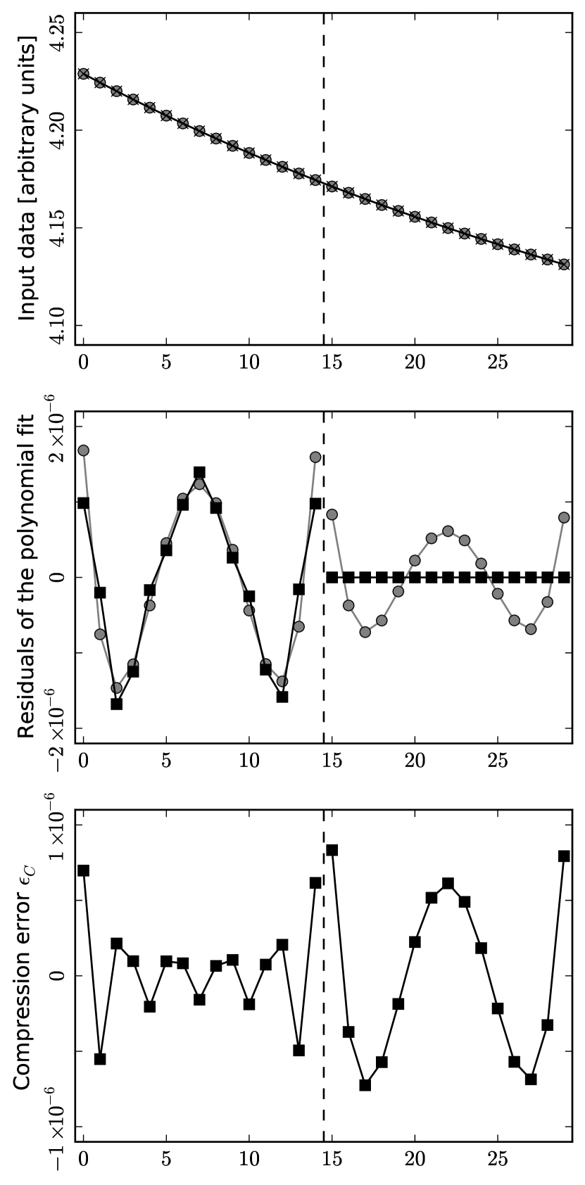
Figure 3 illustrates the application of this compression scheme to some test data.
The decompression is straightforward:
-
1.
Read the coefficients of the polynomial for the first chunk and computes the set of points ;
-
2.
If no Chebyshev coefficients are available, the decompressed data are ;
-
3.
If Chebyshev coefficients are available, produce a sequence of values by filling empty positions with zeroes.
-
4.
Compute using the inverse Chebyshev transform formula (Eq. 7). The decompressed data for this chunk are
(14) -
5.
Iterate over the remaining chunks.
Decompression is faster than compression, as there is no need to compute a linear square fit to find the polynomial : the most computationally intensive operations are the evaluation of the polynomial at points and (when necessary) the computation of the inverse Chebyshev transform, which is done using the FFTW 3 (Fastest Fourier Transform in the West) library (Frigo 1999).
The values and are input parameters for the compressor and need to be properly tuned, in order to produce the desired compression ratio. Their optimization can be tricky, as a number of factors must be considered in choosing them:
-
1.
Generally, the larger and , the better the compression ratio.
-
2.
Large numbers for can produce round-off errors. Such errors are detected by polycomp, but they force the program to degrade the compression ratio by saving more and more Chebyshev coefficients in order to correct the interpolation.
-
3.
Large values of increase significantly the time required for the polynomial fitting and the direct/inverse Chebyshev transforms.
There are several ways to tackle the problem of tuning a lossy compression algorithm. They depend on the nature of the data and the kind of analyses that are expected to be performed on the data themselves. In some cases, it is possible to derive an analytical model that can predict the best values to be used for the parameters. For instance, Shamir and Nemiroff (2005) propose a lossy compression algorithm for astronomical images used for photometry, and it provides a set of equations to quantify the impact of the loss of information to quantities commonly used in photometric analyses. If the development of a theoretical model for the compression is too complex, the most common approach is to estimate the error induced on the results of the data analysis when compressed data are used instead of the original uncompressed ones. For a few examples of the latter approach, see e.g., Vohl et al. (2015); Löptien et al. (2016).
Considering the broad target of this paper, it would be too impractical to provide analytical models to forecast the impact of compression errors to every conceivable scientific product obtained using data compressed with polycomp. However, the program provides two tools which can ease the choice of the best compression parameters for polynomial compression:
-
1.
A slow optimization mode, where polycomp tries a set of pairs provided by the user and picks the one with the best compression ratio;
-
2.
A fast optimization mode, where polycomp requires a pair of values as a starting point, and it uses the algorithm proposed by Nelder and Mead (1965) to find the configuration with the best .
In both cases, the upper bound on the compression error must be passed to the optimizer as an input. In Sect. 3, I will present some examples of this optimization, and I will discuss a few important caveats to be kept in mind when optimizing the polynomial compression. A few more technical details about libpolycomp are provided in A.
2.4 Quantifying the relative importance of the polynomial fitting and of the Chebyshev transform
Depending on the kind of data to compress and on the compression parameters and , the role of Step 4 in the polynomial compression algorithm (Sect. 2.3) might be of greater or lesser importance to determine the overall compression ratio. We can consider two extreme cases: (1) the required is so large that Step 4 is never applied; (2) the required is so small that all chunks must be saved uncompressed (Step 5).
A practical way to quantify the importance of the Chebyshev transform in the polynomial compression is to compare the compression ratio with the one achieved using a simpler algorithm which skips Step 4 completely. In the latter algorithm, if the residuals calculated in Step 3 are too large, the chunk is always saved in uncompressed form, and no Chebyshev transform is ever calculated. I call this algorithm simple polynomial compression. The library libpolycomp implements the simple compression algorithm as well. In Sect. 3, I use this feature to assess the importance of the Chebyshev transform step in the examples considered in this paper.
2.5 Other compression algorithms
The compression algorithms presented so far are specialized for very particular kinds of datasets. The polycomp program can interface to two widely used, general-purpose compression libraries in those cases where none of the algorithms described above are suitable:
-
1.
The zlib library, which implements a variant of the LZ77 algorithm called DEFLATE121212http://www.zlib.net/feldspar.html.;
-
2.
The bzip2 library, which implements a combination of the Burrows-Wheeler algorithm and Huffman coding.
3 Compression performance
In this section I will discuss two applications of the polynomial compression algorithm described in Sect. 2, and I compare its performances with other algorithms.
3.1 Ephemerides
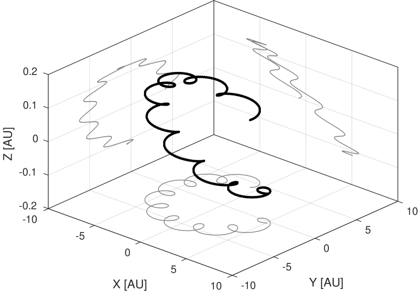
I have used polycomp to compress ephemeris data for Ganymede, one of Jupiter’s moons. Ephemeris tables are a natural input for polynomial compression, as they are usually smooth in nature (provided that the sampling frequency is not too low). The trajectory of Ganymede in the 3-D space as seen from an observer located in Milan (longitude 9.1912∘, latitude 45.4662∘, altitude 147 m) is shown in Fig. 4. I consider the interval of time spanning the interval since January, 1st 2002 till December, 31st 2010. I obtained the ephemeris table using JPL’s HORIZONS system131313http://ssd.jpl.nasa.gov/?ephemerides.. The dataset used for this analysis contains the time (a Julian Date) and the position , measured in AU. These quantities are sampled every 10 min. I have saved such data into a FITS file containing one binary HDU with four 64-bit floating-point columns. The file contains 473 328 rows, and its size is 14.45 MB. It is not easily compressed by standard tools like gzip and bzip2: the compression ratio in these cases is 1.31 and 1.28, respectively, using the -9 command-line switch to force both programs to achieve the best possible compression.
To compress the dataset using polycomp, I have chosen polynomial compression for all the four columns. Since this is a lossy compression, it is necessary to set the upper bound on the compression error (Eq. 2). I used for the Julian time, corresponding to an error of the order of 10 s, and for each of the three coordinates , , and . The bounds for , , and are probably stricter141414The precision of HORIZONS estimates is time-dependent; according to the documentation, “uncertainties in major planet ephemerides range from 10 cm to 100+ km” (http://ssd.jpl.nasa.gov/?horizons_doc#limitations). than the average precision of HORIZONS’ ephemerides: they have been chosen because of their interesting properties in the characterization of the polynomial compression algorithm.
| JD | 50 000 | 2 | 10 518.40 | 10 518.40 |
|---|---|---|---|---|
| 360 | 23 | 11.53 | 4.86 | |
| 360 | 22 | 11.63 | 4.64 | |
| 400 | 22 | 13.79 | 13.79 |
Given the straightforward behaviour of the JD datastream, I avoided the application of a full optimization procedure for the compression parameters and used , . As the data are neatly fitted by a straight line, the compressor does not need to apply any Chebyshev transform, and therefore the full algorithm and the simple compression show the same performance. The expected value for is
| (15) |
while the measured value for is about 10 500.
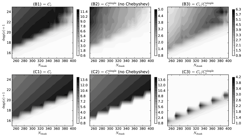
For , , and , I used the optimization mode provided by polycomp to find the parameters of the compressor that produce the best compression ratio . I explored the region of the parameter space generated by the following numbers:
| (16) | ||||
| (17) |
In Fig. 5, I show the result of the exploration of the compression parameter space for a selected number of cases. In the three plots in Row A, I show the difference between the performance of the polynomial compression algorithm versus the simple algorithm when applied to the dataset. The advantage of the former over the latter is evident; the same behaviour is observed with the data in the dataset , which are not shown here. Row B shows that in the case of the dataset the Chebyshev step does not give significant advantages over simple compression: as a matter of fact, the best compression ratio in the two cases is the same, as shown in Table 1. This is a general property of the polynomial compression algorithm: for sufficiently relaxed constraints on , the Chebyshev transform does not provide any advantage over a plain polynomial fitting compression. In the case of the data, this would have been the case if had been set to instead of .
The size of the compressed file is 795.9 kB, thus . This is a substrantial improvement over the simple compression algorithm, which produces a 1681.9 kB file, with . On the other hand, if , then the size shrinks down to 615.9 kB, with : in this case, the simple and polynomial compression schemes produce files of the same size because of the reasons stated above.
3.2 Planck/LFI pointing information
| Datum | Data format | Compression algorithm |
|---|---|---|
| On-board time | 64-bit signed integer | Differenced RLE |
| (colatitude) | 64-bit floating point | Polynomial compression |
| (longitude) | 64-bit floating point | Polynomial compression |
| (orientation) | 64-bit floating point | Polynomial compression |
| Temperature | 64-bit floating point | Quantization |
| Flags | 16-bit integer | RLE |
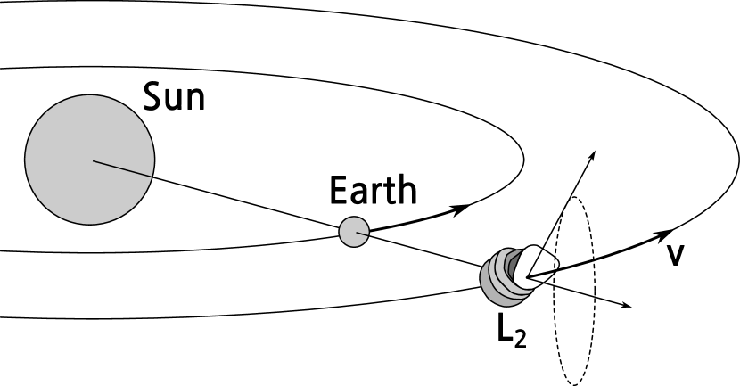
In this section, I study the application of the compression algorithm presented in Sect. 2 to the timelines of the LFI instrument onboard the Planck spacecraft (Planck Collaboration 2015). The LFI (Low Frequency Instrument) is an array of cryogenically cooled HEMT radiometers which observe the sky at three different frequencies: 30, 44, and 70 GHz . The timelines recorded by the instrument are publicly available through the Planck Legacy Archive151515http://www.cosmos.esa.int/web/planck/pla. (PLA); each timeline contains the on-board time, the orientation in the sky of the radiometer’s beam, the temperature measured by the radiometer, and a set of quality flags. A relevant fraction of the Planck timelines () contains the information about the pointing direction of the instruments: I refer to such data as pointing information, or pointings. Pointing information can be encoded either as a set of angles or as length-one vectors, and it can typically take171717Other information recorded in the timelines usually include the timing itself, the scientific datum, and various flags. In the case of the Planck/LFI timelines available on the Planck Legacy Archive161616http://pla.esac.esa.int. (PLA), the timing and the scientific datum take 8 bytes each, while flags require 4 bytes each. On the other side, the pointing information is encoded using three angles , , and , for a total of 24 bytes. So, 24 bytes out of 44 are needed for the angles. Additional housekeeping timelines like bias currents and instrument temperatures are saved at a much lower sampling rate, and they are not an issue. 50 % of the overall space needed by the timelines. The dependence of the LFI beam orientation on time depends on the scanning strategy employed by Planck, which is sketched in Fig. 6.
Pointing information is usually reconstructed using the information about the placement and orientation of the instrument with respect to some reference frame (e.g., the barycentre of the spacecraft), as well as detailed information about the placement of the instrument itself with respect to the center of the reference frame. In some cases, it is enough to combine the line-of-sight vector with the attitude information in order to retrieve the pointing information at any given time181818For instance, this is the approach followed by the WMAP team in publishing the WMAP timelines, see http://lambda.gsfc.nasa.gov/product/map/current/m_products.cfm.. However, for instruments with moderate angular resolution and high sensitivity like LFI, a number of systematic effects that need to be taken into account (stellar aberration, variation in the placement of the optically sensitive parts of the instrument due to thermal dilation, etc.) can lead to non-trivial algorithms to reconstruct the pointing information. (See Planck Collaboration ES (2015), which details the pipeline used for reconstructing the Planck pointing information.) In such cases, saving the computed pointings alongside the scientific data is the best solution for allowing the scientific community to easily use the timelines. This is the approach followed by the PLA.
I characterize here the application of libpolycomp’s algorithm to the whole set of Planck/LFI timelines (4 years of data), in terms of the compression ratio (eq. 1). Details about the data formats and the compression algorithms used in the analysis are reported in Table 2. The layout of the columns used in the input FITS files differs from the layout used by the PLA, as each PLA FITS file contains data acquired by all the radiometers with the same central frequency, and therefore it saves only one copy of the “On-board time” column. Since it is usually more handy to analyze each radiometer separately, I split each PLA file into FITS files, each containing data for one of the radiometers working at the specified frequency ( is 12, 6, and 4 at 70, 44, and 30 GHz respectively); this is the same format used internally by the LFI data processing pipeline. The amount of disk space occupied by the sets of files is 6.5 TB.
| C. freq. | [Hz] | Radiometer | |
|---|---|---|---|
| 70 GHz | 12 | 78.8 | LFI18M |
| 44 GHz | 6 | 46.5 | LFI24M |
| 30 GHz | 4 | 32.5 | LFI27M |
I have applied the compression algorithms provided by polycomp to the pointing and scientific information of three out of the 22 LFI radiometers, namely LFI18M (70 GHz), LFI24M (44 GHz), and LFI27M (30 GHz). The three radiometers sample the sky temperature with different frequencies: 78.8 Hz (LFI18M), 46.5 Hz (LFI24M), and 32.5 Hz (LFI27M).
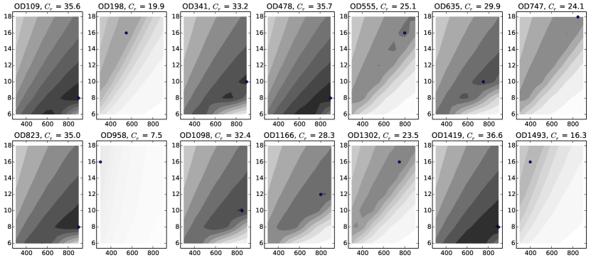
Choosing the optimal compression strategy for the pointing information is not trivial, as there are 1452 files per radiometer, each corresponding to one Operational Day (OD), and each file has the pointing information encoded in three columns: (Ecliptic colatitude), (Ecliptic latitude), and (orientation of the beam). Therefore, the compressor must be tuned separately for each column. Moreover, since Planck’s scanning strategy varies with time, the best values for the two polynomial compression parameters, and , change with time. For instance, Fig. 7 shows contour plots of the value of as a function of and for a set of fourteen randomly-chosen days, when polycomp is applied to the set of colatitudes for radiometer LFI18M.
To determine the best parameters for the compressor, I used the optimization function in the pypolycomp Python library to write a script that implemented a two-stage search strategy:
-
1.
I sampled the parameter space using a wide but coarse grid:
(18) To quicken the process, during this process I used only the first two hours of data for each day.
-
2.
After the first run, I ran the optimizer again on a narrower, finely-gridded area around the point with the best that has been found in the previous run, this time using the full, one-day-long dataset.
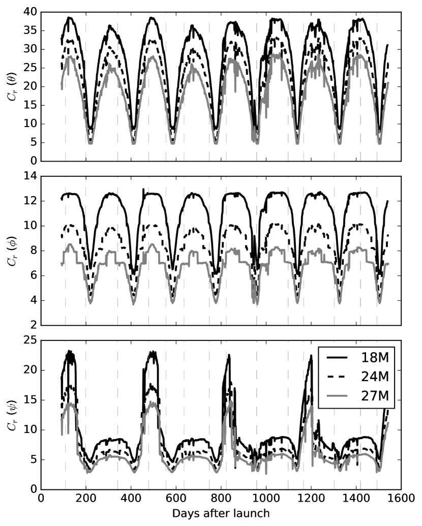
Fig. 8 shows the compression ratio for all the combinations of 1452 operational days (ODs), three angles, and three radiometers considered in this work. There are periodic drops of the compression ratio, and these usually occur at the end of a complete survey of the sky: they are related to quick changes in the asset of the instrument.
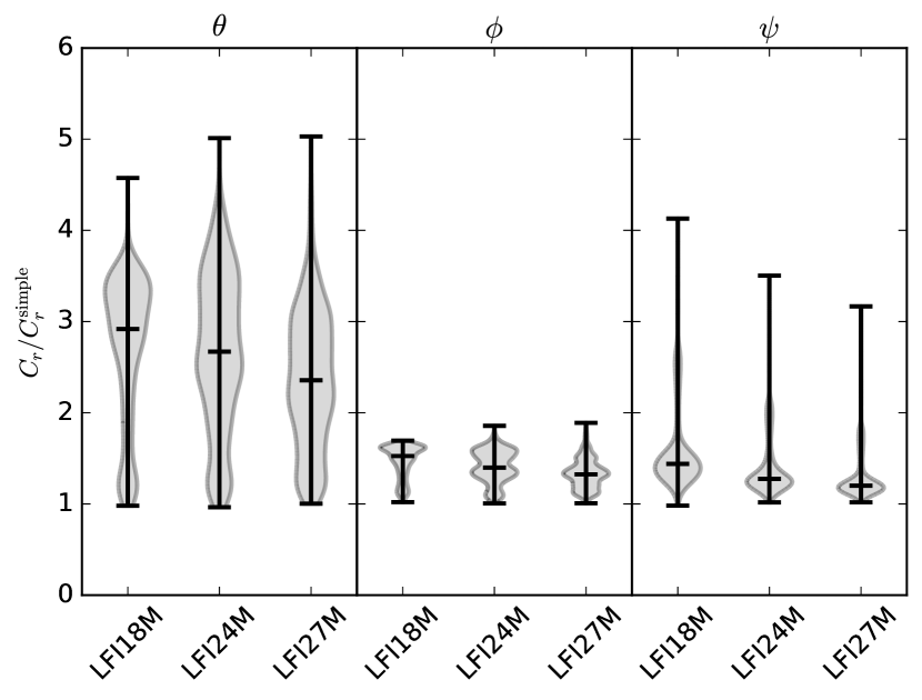
To determine the effectiveness of the Chebyshev transform in improving the compression ratio as compared to the simple algorithm described in Sect. 2.4, I have re-run the optimization for all the data using the simple polynomial compression algorithm. The comparison between the of each best solution in the two cases (polynomial compression versus simple compression) is shown in Fig. 9. The advantage of the polynomial compression algorithm over the simple algorithm is evident expecially in the three datasets.
I have compressed only three out of 22 LFI radiometers. It is possible to extend this result to forecast the expected compression ratio on all the radiometers. The pointing information of the other 19 radiometers is very similar to one of these, because the Planck focal plane moves rigidly. Therefore, the results obtained for these three radiometers can be generalized to the whole set. Assuming that the overall compression ratio of the three radiometers are representative of all the radiometers with the same sampling frequency, it is easy to derive the following formulae
| (19) | ||||
| (20) | ||||
| (21) | ||||
where is the number of radiometers at frequency , is the sampling frequency, is the number of bits used to encode each sample (its value is assumed to be the same for the uncompressed and compressed sequences), is the acquisition time, roughly equal to four years, and is the compression ratio of the whole FITS file, assumed to be the same for all the radiometers. Substituting the values of found for LFI18M, LFI24M, and LFI27M into Eq. (21) leads to the result
| (22) |
as , , and . Since the space needed to keep LFI timelines in uncompressed FITS files is of the order of 7 TB, this means that compressing such timelines using libpolycomp would produce an archive slightly smaller than 800 GB.
4 Impact of the compression in the analysis of Planck/LFI time series
In the previous section I analyzed the performance of the compression schemes presented in Sect. 2, in terms of the compression ratio (Eq. 1). However, two other important parameters which quantify the performance of the compression are: (1) the difference between compressed and uncompressed samples, whose upper bound is , defined in Eq. 2, and (2) the time required to compress and decompress the data. In this section I discuss the quantification of such parameters in the compression of the LFI TOIs discussed in Sect. 3.2.
4.1 Compression error in the LFI TOI pointing angles
I discuss here a few statistical properties of the error in the compression of the samples measuring the three pointing angles (Ecliptic colatitude), (Ecliptic latitude), and (orientation) for the three LFI radiometers considered in Sect. 3.2.
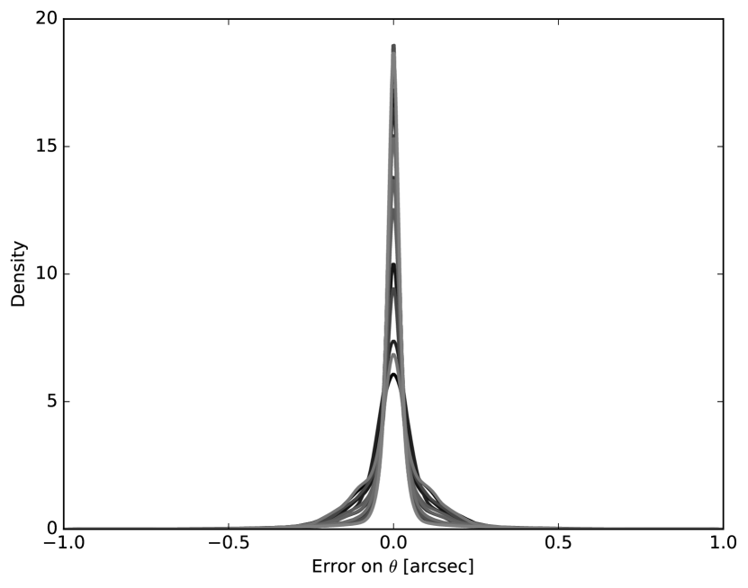
My analysis considered the difference between the -th sample and the compressed value :
| (23) |
For each of the three radiometers I characterized the statistical properties of each of the 1452 datasets (one per operational day) in terms of the following quantities:
-
1.
Maximum and minimum value;
-
2.
Median;
-
3.
First and third quantiles.
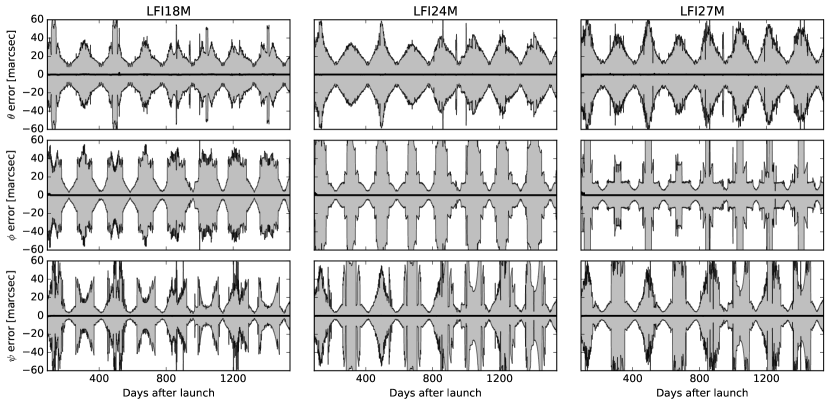
I computed the maximum and minimum value only as a way to test the correctness of the implementation of the algorithm, as the polynomial compression algorithm ensures that (12). The values of the median and the quantiles are shown in figure 10. The average error (median) is consistent with zero in every case, and the inter-quartile range is of the order of tens of milliarcseconds, thus at least one order of magnitude smaller than the upper bound set for the compression error of the three LFI pointing angles. The statistical distribution of the errors is not normal, since it is bounded by by definition; it is sharply peaked around zero, and it shows a remarkable level of simmetry: the difference between the mean error and the median error, as well as the skewness of the error, is of the order of a few tens of arcsecond at most for all the ODs considered in the analysis.
4.2 Number of hits per pixel in sky maps
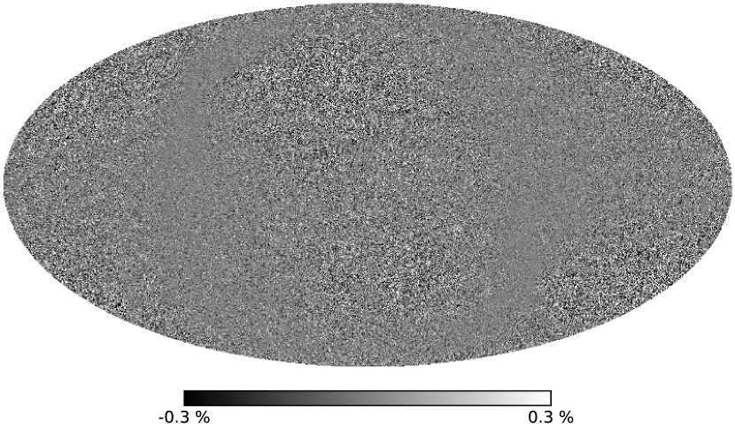
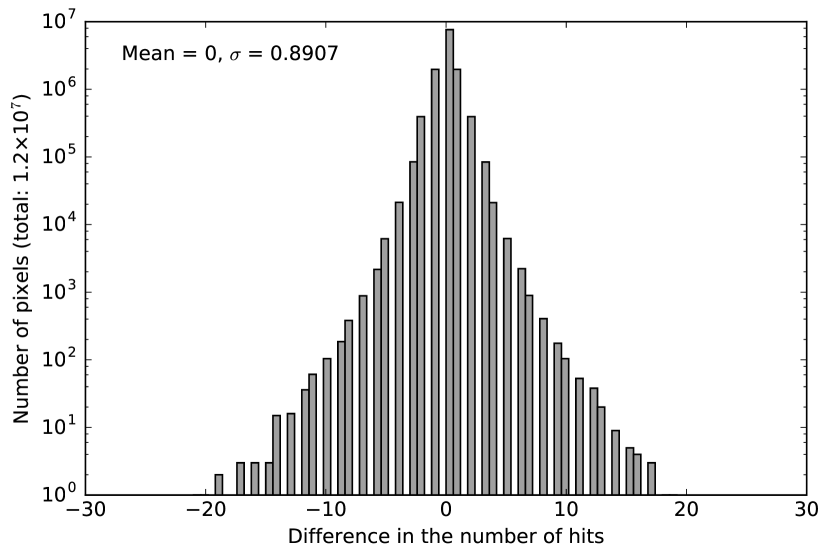
The purpose of measuring timelines using Planck/LFI is to project each sample on the sky sphere and produce a map of the full sky. Since this process requires the sky sphere to be discretized into a set of pixels (the Planck collaboration uses the Healpix pixelization scheme, see Górski et al. 2005), the value of each pixel will be the combination of the value of one or more samples. The number of samples used to determine the value of a pixel is the hit count of the pixel. This quantity has a number of applications (e.g., white noise characterization, destriping), and it is thus interesting to determine if the compression errors in the pointing information alter the hit count significantly.
I have compared hit count maps produced using the original, uncompressed pointings with the same map produced using compressed pointings. Results are shown in Figs. 12 and 13. Mismatches have zero mean and average, and the overall level of the mismatch is small. The maps use the Healpix pixelization scheme (Górski et al. 2005), with a resolution of (), the same resolution as the nominal Planck maps.
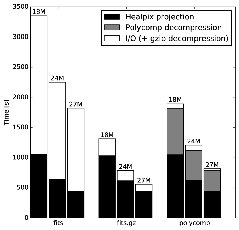
I have profiled the execution of the script which creates the hit maps, in order to measure the time required to run the following operations:
-
1.
Loading data from FITS files via calls to cfitsio (Pence 2010);
-
2.
Decompressing data using libpolycomp (when applicable);
-
3.
Projecting the pointings on the sky and creating the map, using my own implementation of Healpix projection functions (Górski et al. 2005).
I run this test on Numenor191919http://www.mi.infn.it/~maino/erebor.html., a 96-core cluster of Intel Xeon processors hosted by the Physics department of the Università degli Studi in Milan. Each run allocated 12 OpenMP processes for libpolycomp. After having created the hit maps from the pointings stored in polycomp files, I repeated the test twice, reading pointing information that was stored in (1) uncompressed FITS files, (2) gzip-compressed FITS files. Because of the way cfitsio reads data, I did not use Planck PLA files: since FITS binary tables are stored in row-major order and cfitsio disk reads are buffered in chunks of 2880 bytes, reading only a few columns in a PLA file would require cfitsio to load all the six columns in the table HDU from disk. Therefore, I created a new set of FITS files containing only the THETA and PHI columns, and read them in chunks of rows, where is the return value of the fits_get_rowsize function: this reduces the I/O time for uncompressed FITS files by a factor with respect to the case where and are loaded from PLA files via two calls to fits_read_col. No such trick is required when the code loads polycomp files, as each column is stored in its own HDU.
The results of the three tests are shown in Fig. 14. Using polycomp files represents a clear advantage over uncompressed FITS files, but the fastest case is when gzip-compressed files are loaded. In this case, cfitsio decompresses the file in memory and no longer accesses the disk. The disadvantage of using gzipped FITS files is that the compression ratio is quite poor: for all the three frequencies, .
5 Conclusions
In this paper I have presented the result of three activities:
-
1.
The description of an algorithm for the compression of smooth data series which approximates data through the sum of least-squares polynomials and Chebyshev polynomials;
-
2.
The implementation of a program, polycomp, which compresses data series using the algorithm in point 1 as well as other well-known compression algorithms;
-
3.
A characterization of polycomp’s ability to compress Planck/LFI time ordered information, both in terms of the compression ratio (Eqs. 1 and 3) and of the compression error (Eq. 2). Given some reasonable upper bound to the compression error, the achieved compression ratio is greater than 8. I have also estimated the impact of the compression error on a few quantities relevant for the analysis of the Planck/LFI data.
The results presented in this paper might find interesting application in the development of techniques for the storage of data acquired by future space missions. An example is the proposed LiteBird mission (Matsumura et al. 2014), which will be devoted to the measurement of CMB polarization anisotropies in the 50-320 GHz range: the instrument will be made by 100 times many sensors as Planck/LFI and is therefore likely have significant demand in terms of data storage.
Aknowledgements
The author would like to thank Michele Maris for having introduced him into the world of astronomical data compression, and Marco Bersanelli and the two anonymous referees for the useful comments which helped to improve this paper and the libpolycomp library.
References
References
- Briggs and Henson (1995) Briggs, W., Henson, V., 1995. The DFT: An Owners’ Manual for the Discrete Fourier Transform. Society for Industrial and Applied Mathematics. doi:10.1137/1.9781611971514.ch8.
- Frigo (1999) Frigo, M., 1999. A fast fourier transform compiler, in: Proceedings of the ACM SIGPLAN 1999 Conference on Programming Language Design and Implementation, ACM, New York, NY, USA. pp. 169–180. doi:10.1145/301618.301661.
- Górski et al. (2005) Górski, K.M., Hivon, E., Banday, A.J., Wandelt, B.D., Hansen, F.K., Reinecke, M., Bartelmann, M., 2005. HEALPix: A Framework for High-Resolution Discretization and Fast Analysis of Data Distributed on the Sphere. The Astrophysical Journal 622, 759–771. doi:10.1086/427976, arXiv:0409513.
- Jurić et al. (2015) Jurić, M., Kantor, J., Lim, K., Lupton, R.H., Dubois-Felsmann, G., et al., 2015. The LSST Data Management System. ArXiv e-prints arXiv:1512.07914.
- Kizner (1967) Kizner, W., 1967. The Enhancement of Data by Data Compression Using Polynomial Fitting. Technical Report 32-1078. Jet Propulsion Laboratory. Pasadena, California.
- Laureijs et al. (2011) Laureijs, R., Amiaux, J., Arduini, S., Auguères, J.., Brinchmann, J., Cole, R., Cropper, M., Dabin, C., Duvet, L., Ealet, A., et al., 2011. Euclid Definition Study Report. ArXiv e-prints arXiv:1110.3193.
- Löptien et al. (2016) Löptien, B., Birch, A.C., Duvall, T.L., Gizon, L., Schou, J., 2016. Data compression for local correlation tracking of solar granulation. A&A 587, A9. doi:10.1051/0004-6361/201526805.
- Matsumura et al. (2014) Matsumura, T., Akiba, Y., Borrill, J., Chinone, Y., Dobbs, M., et al., 2014. Mission design of litebird. Journal of Low Temperature Physics 176, 733--740. doi:10.1007/s10909-013-0996-1.
- Nelder and Mead (1965) Nelder, J.A., Mead, R., 1965. A simplex method for function minimization. The Computer Journal 7, 308--313. doi:10.1093/comjnl/7.4.308.
- Norris (2010) Norris, R., 2010. Data challenges for next-generation radio telescopes, in: e-Science Workshops, 2010 Sixth IEEE International Conference on, pp. 21--24. doi:10.1109/eScienceW.2010.13.
- Ohtani et al. (2013) Ohtani, H., Hagita, K., Ito, A.M., Kato, T., Saitoh, T., Takeda, T., 2013. Irreversible data compression concepts with polynomial fitting in time-order of particle trajectory for visualization of huge particle system. Journal of Physics: Conference Series 454, 012078. URL: http://stacks.iop.org/1742-6596/454/i=1/a=012078.
- OpenMP Architecture Review Board (2011) OpenMP Architecture Review Board, 2011. OpenMP Application Program Interface. Specification. URL: http://www.openmp.org/mp-documents/OpenMP3.1.pdf.
- Pence (2010) Pence, W.D., 2010. CFITSIO: A FITS File Subroutine Library. Astrophysics Source Code Library. arXiv:1010.001.
- Pence et al. (2010) Pence, W.D., Chiappetti, L., Page, C.G., Shaw, R.A., Stobie, E., 2010. Definition of the flexible image transport system (fits), version 3.0. A&A 524, A42. doi:10.1051/0004-6361/201015362.
- Pennebaker and Mitchell (1992) Pennebaker, W.B., Mitchell, J.L., 1992. JPEG Still Image Data Compression Standard. Springer US.
- Philips and De Jonghe (1992) Philips, W., De Jonghe, G., 1992. Data compression of ecg’s by high-degree polynomial approximation. Biomedical Engineering, IEEE Transactions on 39, 330--337. doi:10.1109/10.126605.
- Planck Collaboration (2015) Planck Collaboration, 2015. Planck 2015 results. I. Overview of products and results. A&A, accepted arXiv:1502.01582.
- Planck Collaboration ES (2015) Planck Collaboration ES, 2015. The Explanatory Supplement to the Planck 2015 results, http://wiki.cosmos.esa.int/planckpla/index.php/Main_Page. ESA.
- Salomon (2006) Salomon, D., 2006. Data Compression: The Complete Reference. Springer-Verlag New York, Inc., Secaucus, NJ, USA.
- Shamir and Nemiroff (2005) Shamir, L., Nemiroff, R.J., 2005. Photzip: A lossy fits image compression algorithm that protects user-defined levels of photometric integrity. AJ 129, 539–546. doi:10.1086/426363, arXiv:astro-ph/0410212.
- Stoehr et al. (2014) Stoehr, F., Lacy, M., Leon, S., Muller, E., Manning, A., Moins, C., Jenkins, D., 2014. The alma archive and its place in the astronomy of the future. doi:10.1117/12.2055539, arXiv:1504.07354.
- Vohl et al. (2015) Vohl, D., Fluke, C., Vernardos, G., 2015. Data compression in the petascale astronomy era: A gerlumph case study. Astronomy and Computing 12, 200–211. doi:10.1016/j.ascom.2015.05.003.
Appendix A Implementation of polycomp
I have implemented the algorithms described in this paper in a BSD-licensed C library, libpolycomp202020https://github.com/ziotom78/libpolycomp.. I have also implemented a set of Python 3 bindings to the library, available in a separate repository (https://github.com/ziotom78/polycomp). The Python library includes a stand-alone program, polycomp, which can compress/decompress ASCII and binary tables saved in FITS files.
The libpolycomp library has been implemented using the 1989 definition of the C standard, and it should therefore be easily portable to different compilers. The author tested it using the following compilers:
-
1.
GNU gcc212121https://gcc.gnu.org/. 4.9 and 5.1;
-
2.
clang222222http://clang.llvm.org/. 3.4 and 3.5;
-
3.
Intel C Compiler232323https://software.intel.com/en-us/c-compilers. 16.0.
The library uses OpenMP (OpenMP Architecture Review Board 2011) to take advantage of multiple-core systems. It has been fully documented, and the user’s manual242424http://ziotom78.github.io/libpolycomp/. is available online. The library API has been designed in order to be easily callable from other languages.
The Python wrappers have been built using Cython252525http://cython.org/., and the polycomp program is able to save the compressed timestreams in files. The format of these files is based on the FITS file format (Pence et al. 2010), and it is fully documented in the polycomp user’s manual262626http://polycomp.readthedocs.org/en/latest/..