Roughening of an interface in a system with surface or bulk disorder.

Abstract

We study numerically the roughening properties of an interface in a two-dimensional Ising model with either random bonds or random fields, which are representative of universality classes where disorder acts only on the interface or also away from it, in the bulk. The dynamical structure factor shows a rich crossover pattern from the form of a pure system at large wavevectors $k$, to a different behavior, typical of the kind of disorder, at smaller $k$’s. For the random field model a second crossover is observed from the typical behavior of a system where disorder is only effective on the surface, as the random bond model, to the truly large scale behavior, where bulk-disorder is important, that is observed at the smallest wavevectors.

I Introduction

Interface roughening is a widely observed feature occurring in many fields of science ranging from physics to engineering and biology, including crystal growth, viscous flow in porous media and many other phenomena 15pleim .

Although interfaces may roughen also in the absence of disorder, a great deal of interest has been recently payed to those systems whose properties are determined by the presence of impurities or other sources of quenched randomness. Typical examples are found in high-Tc superconductors da45a51pleim , and disordered magnets refscrp . In these systems the properties of the interfaces are mainly due to the interplay between their elasticity and the localization effects due to the impurities. In a superconductor, the bending of magnetic flux lines is due to the competition between defects pinning (grain boundaries, oxygen impurities etc.) and the bending energy 4kard . Similarly, the geometry of domains walls in disordered ferromagnets originates from the balance between the energy gain associated to interface deformations caused by random impurities and the surface tension cost. This mechanism produces peculiar equilibrium and non-equilibrium properties 5kard .

A great advance in roughening theory has been achieved by the recognition that a scaling symmetry, analogous to the one at work in ordinary critical phenomena, underlies the properties of interfaces familvick . According to this hypothesis, when roughness develops in an initially smooth interface at time $t=0$, the evolution of the structure factor [see around Eq. (5) for a precise definition of this quantity] takes the form

$$S(k,t)\simeq k^{-(1+2\zeta)}f[k\xi(t)],$$ (1)

where $k$ is the wavevector, $\zeta$ is the roughness exponent, $\xi(t)$ has the physical dimensions of a length and $f$ is a scaling function. The behavior of these quantities and, in particular, of the roughness exponent, are expected to exhibit universal properties. One of the relevant features determining the universality classes is the presence of quenched disorder. Indeed, in many cases it is found to modify the properties of the interfaces with several consequences on the materials properties, as it is observed, for instance, in the growth of a magnetic phase refscrp2 .

Not only the presence of quenched randomness is relevant, but also its nature. An important distinction exists natterman between systems where disorder acts only at the interfaces (interface disorder) and others where it is effective also in the regions away from them (bulk disorder). Systems belonging to these two classes are all expected to obey Eq. (1) but with different roughening exponents and properties of $\xi$ and $f$.

In this paper we investigate numerically the behavior of a one-dimensional interface evolving in a two-dimensional random medium. The random bond and the random field Ising models are taken as prototypical of systems with interface disorder and with bulk disorder, respectively. By computing the structure factor we show the existence of a crossover from pure to interface-disorder behavior or from pure to bulk-disorder behavior as the wave vector is changed. Usually refscrp2 , to randomness is associated a characteristic length $\lambda$, and the crossover from pure to disorder-dominated behavior takes place as the observation length scale grows from smaller to larger than $\lambda$. Indeed, this is the pattern observed in the interface disorder case, i.e. with random bonds, where the structure factor is pure-like in the wave vector range $k\gg\lambda^{-1}$ and departs from pure behavior for $k\ll\lambda^{-1}$. Instead, the crossover in the bulk disorder case due to the random fields is novel and more interesting. In fact, the data can be accounted for by introducing an additional characteristic length scale $\Lambda>\lambda$, such that the crossover pattern displays pure behavior for $k\gg\lambda^{-1}$, interface-disorder behavior for $k$ in between $\Lambda^{-1}$ and $\lambda^{-1}$, and bulk-disorder behavior for $k\ll\Lambda^{-1}$. In particular, in the intermediate regime the roughness exponent takes the value ($\zeta=2/3$ natterman ; dueterzi ) expected for a system with interface-disorder. Truly large-scale properties are only displayed on lengthscales larger than $\Lambda$, where the asymptotic value of the roughness exponent takes the value expected in a system with bulk disorder ($\zeta=1$ natterman ).

The paper is organized in five sections: In Sec. II we introduce the random bond and the random fields Ising models. In Sec. III we consider, preliminarly, the pure case in order to have a reliable benchmark to compare with, particularly for what concerns the relevance of finite size effects. Sec. IV is devoted to the study of the disordered cases and to the discussion of what is observed. In Sec. V we summarize the main results. An appendix contains a further discussion of the finite-size effects of the model.

II The model

We consider a ferromagnetic system described by the Hamiltonian

$${\cal H}(\{S_{i}\})=-\sum_{\langle ij\rangle}J_{ij}S_{i}S_{j}+\sum_{i}H_{i}S_{i},$$ (2)

where $S_{i}=\pm 1$ are Ising spin variables defined on a two-dimensional $L\times L$ square lattice and $\langle ij\rangle$ are two nearest neighbor sites. We denote by $x$ ($x=1,2,\dots,L$) and $z$ the coordinates of a site $i$ of the lattice along the horizontal and vertical direction, respectively.

We will study two types of quenched disorder:

i) Random bonds Ising model (RBIM): In this case $H_{i}\equiv 0$ and the coupling constants $J_{ij}$ are independent random numbers extracted from a flat distribution in $[J_{0}-\delta,J_{0}+\delta]$, with $\delta<1$ in order to keep the interactions ferromagnetic and to avoid frustration effects.

ii) Random fields Ising model (RFIM): In this case the ferromagnetic bonds are fixed $J_{ij}\equiv J_{0}$, while the external field at each site $H_{i}=\pm\delta$ is uncorrelated and sampled from a symmetric bimodal distribution.

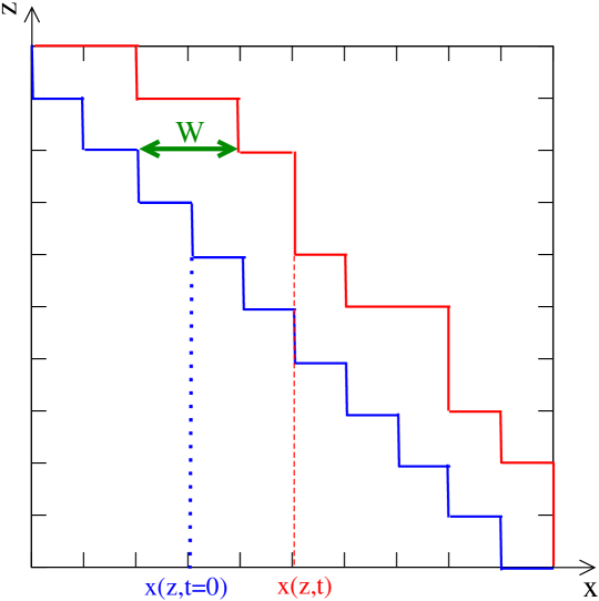
We prepare the system at time $t=0$ by seeding an interface ${\cal I}$ along the diagonal, i.e. we set spins $S_{i}=+1$ in one of the two halves of the system with $z\geq L-x$ and $S_{i}=-1$ in the other, as pictorially shown in Fig. 1. Then, moving horizontally at a given value of $z$, upon increasing $x$ one encounters only one couple of neighboring antiparallel spins $S_{i}S_{j}$ and we define the (horizontal) position $x(z,t=0)$ of the interface as the coordinate $x$ of the first non-aligned spin $S_{i}$.

Figure 1: The position of the interface at time $t=0$ (blue curve on the left) and its evolution at a later time $t$ (red curve on the right) are pictorially sketched. $W(t,\epsilon)$ is of the order of magnitude of average horizontal distance between the two profiles.

A dynamics is then introduced from time $t=0$ onwards by flipping single spins according to Glauber transition rates at temperature $T$

$$w(S_{i}\to-S_{i})=\frac{1}{2}\left[1-S_{i}\tanh\left(\frac{H^{W}_{i}+H_{i}}{T}\right)\right]$$ (3)

where

$$H^{W}_{i}=\sum_{j\in nn(i)}J_{ij}S_{j}$$ (4)

is the local Weiss field (the sum runs over the nearest neighbours $j$ of $i$).

In order to keep a single spanning interface stable at all times we use anti-periodic boundary conditions and set $J_{0}\to\infty$; this can be implemented practically by forbidding flips of spin away from the interface. Notice that with this choice the equilibrium-state of the Ising model (2) is ferromagnetic at any finite temperature. Furthermore, in this limit the model contains a single parameter $\epsilon=\delta/T$, so in the following we will fix $T=0.01$ and let $\delta$ vary. Since we are interested in the limit $L\to\infty$ of an infinite system we will set $L$ to the largest numerically tractable value. A discussion of unavoidable finite-size effects will be given in the following sections and in the Appendix.

Before proceeding, let us stress the fact that in both model i) and ii) there is no neat drive on the motion of the domain wall, because the average value $\overline{H_{i}}$ of $H_{i}$ vanishes. This is at variance with the frequently studied problem sugref1 ; sugref2 where the depinning of the interface is obtained by raising $\overline{H_{i}}$ above a certain threshold value.

The main dynamical feature of the process is the kinetic roughening of the interface which can be studied by computing the structure factor $S(k,t,\epsilon)$, namely the Fourier transform (with respect to $r$) of the surface correlation function

$$G(r,t,\epsilon)=\frac{1}{L}\int_{0}^{L}\langle u(z,t)u(z+r,t)\rangle_{\epsilon}dz,$$ (5)

where $u(z,t)\equiv x(z,t)-x(z,0)$ is the horizontal displacement of the interface, namely the distance moved from its initial position, and $\langle\cdots\rangle_{\epsilon}$ is a statistical average in the presence of disorder, if present.

The interface roughness $W$ is defined by the autocorrelation function

$$W^{2}(t,\epsilon)=\frac{1}{L}\int_{0}^{L}\langle u^{2}(z,t)\rangle_{\epsilon}dz=G(0,t,\epsilon)$$ (6)

which is obtained from the structure factor as

$$W^{2}(t,\epsilon)=\int\frac{dk}{2\pi}\,S(k,t,\epsilon).$$ (7)

III Pure system

Before studying the effects of quenched disorder it is useful to consider preliminarly the well-known behavior of the structure factor in the pure case. This will serve as a benchmark to tune the methodology and to discuss the presence of finite-size effects.

For a pure system ($J_{ij}\equiv J_{0},H_{i}\equiv 0$) of infinite size, continuum theories upton predict the scaling form (1) for $t$ sufficiently large, $\zeta=1/2$, and a scaling function satisfying the limiting behaviors

$$f(x)=\left\{\begin{array}[]{ll}const.\,,&\mbox{for}\,\,\,x\gg 1\\ x^{1+2\zeta}\,\,,&\mbox{for}\,\,\,x\ll 1\end{array}\right..$$ (8)

This is correct also on a lattice for wavevectors much smaller than the inverse lattice spacing $a^{-1}$. In order to make the extension to all $k$ values the replacement $k\to q=\frac{1}{a}\sqrt{2[1-\cos(ka)]}$ must be made in Eqs. (1,8). This monotonic transformation amounts only to a small deformation at the largest wavevectors and extends the validity of Eq. (1) to the large $k$ domain. Given the very similar role played by $k$ and $q$, we will use the term wavevector also for $q$ (with a minor abuse of language ).

Notice that Eq. (1) holds in an infinite system with $L=\infty$. For all practical purposes the condition $\xi(t)\ll L$ is sufficient to guarantee the infinite-system behavior. Since $\xi(t)$ is a growing length, given a certain system size $L$, this condition is fulfilled for times $t\ll t_{L}$, where $t_{L}$ is such that $\xi(t_{L})\sim L$. As we will discuss further below, in numerical simulations it is important to reach very long times in order to have a good estimate of the asymptotic properties we are interested in, but this implies that finite-size effects may be present. In order to keep these corrections under control, the scaling form (1) must be upgraded to take into account the system’s finite size

$$S(k,t,L)=q^{-(1+2\zeta)}g\left[q\xi(t),qL\right],$$ (9)

where we have replaced $k$ with $q$ as discussed above, and $g(x,y)$ is such that no finite size effects are present for $y=qL\gg 1$, i.e.

$$g(x,y)\simeq f(x)\,,\,\,\,\mbox{for}\,\,\,y\gg 1,$$ (10)

with $f$ the same function of Eqs. (1,8), whereas for $x\gg 1$ (i.e. for large times) $S(k,t,L)$ converges to the equilibrium value $S_{eq}(k,L)$ which explicitly depends on $y$ and determines, using Eq. (7), the saturation to the equilibrium value of the roughness

$$W^{2}(t=\infty,L)=L^{2\zeta},$$ (11)

thus earning $\zeta$ the name roughness exponent.

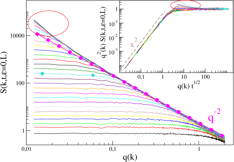
Let us now illustrate how this scaling scenario works. In Fig. 2, the structure factor $S(k,t,L)$ for the pure system is plotted against $q$ for a system of size $L=1024$ and several times $t$. As expected from Eqs. (1,8), in the absence of finite-size effects (i.e. for sufficiently small times $t\leq 92368$) these curves obey the power law $S\sim q^{-2}$ for wavevectors larger than a typical value that we identify with $\xi^{-1}(t)$, and then bend over to a constant for $q\ll\xi^{-1}(t)$. The length $\xi(t)$ can be operatively extracted by asking for the best data-collapse of the scaling function $q^{2}S$ at different times as a function of $q\xi(t)$, yielding the well known result $\xi(t)\sim t^{1/2}$. The data collapse obtained by plotting $q^{2}S$ against $qt^{1/2}$ is shown in the inset of Fig. 2.

The curves for $t\geq 148736$ (largest five times) in Fig. 2 correspond to observation times large enough to reach saturation at $f(x)=const.$ in Eq. (8) in the whole available range of wavevectors. Then one should observe $S\propto q^{-2}$ for all $q$. Instead, these curves bend upward at small wavevectors (for $q\lesssim 0.03$, in a region that has been indicated by an ellipse in Fig. 2)) and depart from the behavior expected in an infinite system. The same effect is observed in the inset of the figure, where data collapse fails at the largest times for small $qt^{1/2}$. This is a finite size effect, since the onset wavevector becomes smaller by increasing the system size $L$. Further evidence for this is given in the Appendix. According to Eq. (9), this means that for such long times $\xi$ is so large to make relevant the second entry of the scaling function $g$, spoiling in this way the infinite system behavior (1,8).

Recalling Eq. (9) it is clear that the roughness exponent can be obtained by fitting the slope $-1+2\zeta$ of the plot of $S$ versus $q$ in the regime where the scaling function $g$ is constant, namely when the wave vector condition

$$q\gg\max\left[\xi^{-1},L^{-1}\right]$$ (12)

is met. In the pure case this amounts to consider the linear envelope of the various curves (for different times) of $S$ versus $q$ in the double-logarithmic plot of Fig. 2. Considering, as an example, the curve at the intermediate time $t=789$ (turquoise with circles) it is clear that the linear envelope is not followed for $q\lesssim 0.2$ because the curve flattens as due to the fact that $q\gg\xi^{-1}$ is no longer obeyed (one can easily be convinced that $\max\left[\xi^{-1},L^{-1}\right]=\xi^{-1}$ in this case by the fact that the typical wavevector where $S$ starts flattening is a decreasing function of time). Operatively, we define the region $q\gg\xi^{-1}$ as the one where the data at a certain time superimpose to those at the immediate earlier times. The situation changes for very large times ($t\geq 35623$, say). For such long times one sees that the linear envelope is no longer followed for $q\lesssim 0.05$. In this case, at variance with what observed for intermediate times (discussion above), there is an initial upward bending of the curves in a region marked by the red ellipse (before flattening to a finite value for $q\to 0$). In this case one has $\max\left[\xi^{-1},L^{-1}\right]=L^{-1}$, as it can be recognized by the fact that the curves for $S$ at different times all depart from the linear envelope around the time-independent value $q\simeq 0.05$ (since, differently from $\xi^{-1}$, $L^{-1}$ is time independent). In conclusion, for any time $t$ one can practically define the $q$-region where the condition (12) is met as that where the data for $S$ superimpose to those at the earlier time and $q\geq 0.05$. We will see in the following that an analogous procedure can be adopted for the cases with disorder.

Figure 2: $S(k,t,\epsilon=0,L)$ is plotted against $q$ for the pure case. Different curves correspond to exponentially increasing times ($t=2,3,5,7,11,18,29,46,73,118,189,304,490,789,1269,$ $2044,3291,5299,8532,13739,$ $22123,35623,57362,92368,148736,239503,385663,621017,10^{6}$ from bottom to top). The bold-dotted magenta line is the power-law $q^{-2}$ expected for an infinite system in the limit $t\to\infty$. The regions encircled by a red ellipse is the one where finite-size effects show-up. In the insets the data collapse obtained by plotting $q^{2}S(k,t,\epsilon=0,L)$ against $qt^{1/2}$ is shown. The brown-dashed line is the power-law $x^{2}$ expected for small $x$ according to Eq. (8).

IV Quenched disorder

As anticipated in the Introduction and as discussed in Ref. refscrp2 , when quenched disorder parametrized by $\epsilon$ is added to a system its effects are usually relevant on lengthscales larger than a certain characteristic length $\lambda(\epsilon)$. For instance, it is clear that introducing a small density $\rho$ of diluted impurities in a pure system cannot change the properties lengthlambdadil on lengthscales much smaller than the typical distance $\simeq\rho^{-1/d}$ between such impurities ($d$ is the spatial dimension), simply because within such small distances the probability to find an impurity is negligible and the system is basically undistinguishable from the pure one. The same situation is found also in models, as the disordered Ising magnets considered here, or bonds, where impurities are not diluted but distributed all over the system, although the physical interpretation of this length might not be straightforward. The presence and the properties of this length in the RBIM and RFIM were discussed in lengthlambdarb and  lengthlambdarf where it was shown that $\lambda$ is a decreasing function of $\epsilon$ with the property

$$\lim_{\epsilon\to 0}\lambda(\epsilon)=\infty.$$ (13)

Since disorder is effective over distances larger than $\lambda$, in an infinite system the pure form (8) of $S$, with $\zeta=1/2$, is expected to be obeyed for $q\gg\lambda^{-1}(\epsilon)$ even in the presence of disorder. In order to check this and other issues that will be addressed below, we have performed a series of simulations of the RBIM and of the RFIM. For the former we have considered a system of size $L=512$, while for the latter we set $L=1024$ for $\epsilon\leq 0.5$, $L=512$ for $\epsilon=0.6$ and $L=256$ for $\epsilon=0.8$. Smaller system sizes are used for the largest values of $\epsilon$ since the dynamics is slower.

Figure 3: $S(k,t,\epsilon,L)$ is plotted against $q$ for the RBIM at $t=10^{7}$ ($t=10^{6}$ for $\epsilon=0$).

Figure 4: $S(k,t,\epsilon,L)$ is plotted against $q$ for the RFIM at $t=10^{6}$ ($t=10^{7}$ for $\epsilon\geq 0.7$). In the inset the effective exponent $\zeta$ obtained by fitting the curves for $q\geq 1$ is plotted against $\epsilon$.

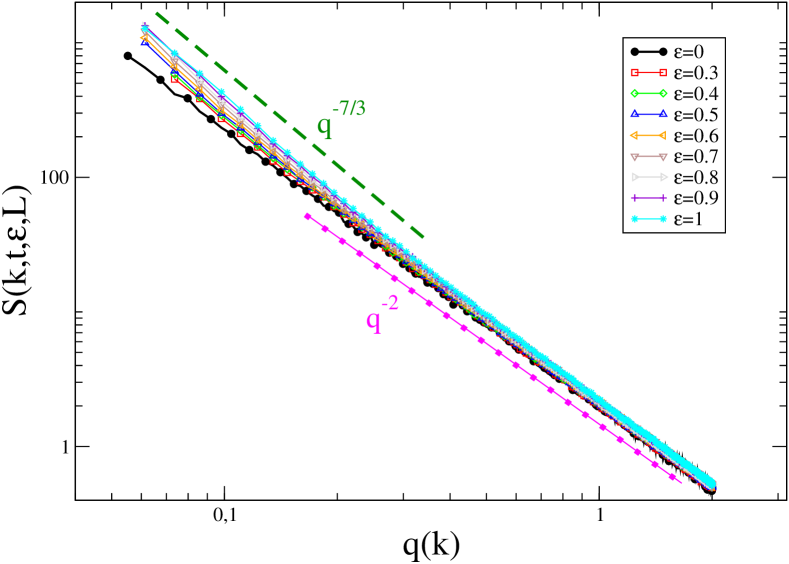
The structure factor for the RBIM is shown in Fig. 3 at time $t=10^{7}$. Here it is observed that $S$ behaves as in the pure system down to wavevectors of order $q\simeq 0.2-0.3$. In particular, in this range, the curves are independent of $\epsilon$ and behave as $q^{-2}$. For smaller values of the wavevector the curves for the disordered system deviate upward from the $q^{-2}$ pure behavior, signaling a crossover to a region where disorder is relevant. Despite the smoothness of the crossover, it can be observed that the curves for large $\epsilon$ depart from the pure behavior at larger wave vectors, and in a more pronounced way. This is because the crossover occurs when $q^{-1}\simeq\lambda(\epsilon)$ and, as discussed above (recall Eq. (13)), the latter is a decreasing function of $\epsilon$. Notice also that for the largest values of $\epsilon$ a small departure from the pure-like behavior can be detected even for the largest wavevectors: starting from $\epsilon=0.9$ the curves appear slightly displaced vertically. This signals the fact that, for these large values of the disorder strength, $\lambda^{-1}$ is already of the order of the largest wave vectors and the effects of an incipient crossover can already be detected. The discussion of $S$ in this range of $q$ where disorder is effective is postponed to Sec. IV.1.

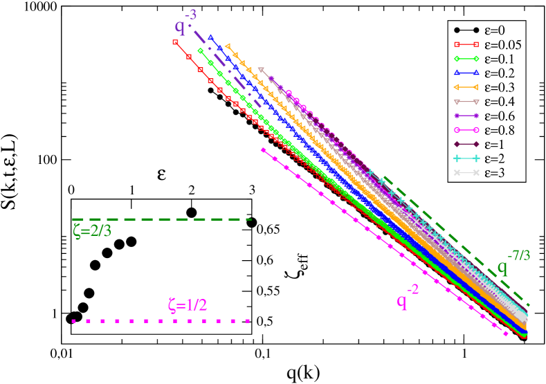
Limited to the large-$q$ sector, a similar behavior of $S$ is observed also in Fig. 4 for the model with random fields. Here we compare the structure factor computed at the longest simulated time ($t=10^{6}$ for $\epsilon\leq 0.6$ or $t=10^{7}$ for $\epsilon=0.8$) for different values of $\epsilon$. When the strength of the disorder is moderate, for $\epsilon\lesssim 0.1-0.2$, the curves for large $q$ superimpose on the one for $\epsilon=0$. However, for smaller wave vectors, they bend upwards very evidently. For larger values of the disorder strength, for $\epsilon\gtrsim 0.3$, the curves start to depart from the pure case already at the largest wave vectors considered. In the same range of values of $\epsilon$ the departure is much larger than in the RBIM and, for the largest value of $\epsilon$ a slope somewhat larger than $q^{2}$ is observed, as will be further commented in Sec. IV.2.

Up to this point we have checked that the pure-like behavior is obeyed also in the presence of a sufficiently small disorder in the large wavevector sector. Since time is very large in Figs. 3,4, in this large-$q$ region one always has $q\xi(t)\gg 1$ and no finite-size effects. In the following we will discuss how the properties of the roughness change for smaller $q$ where the presence of quenched randomness becomes relevant (upward bending of the curves). We still want to focus on the region where condition (12) is satisfied because, according to the discussion of Sec. III in this regime the slope of $S$ directly provides the roughening exponent $\zeta$ we are interested in. However, we have to face the problem that for small $q$ this condition could not be satisfied.

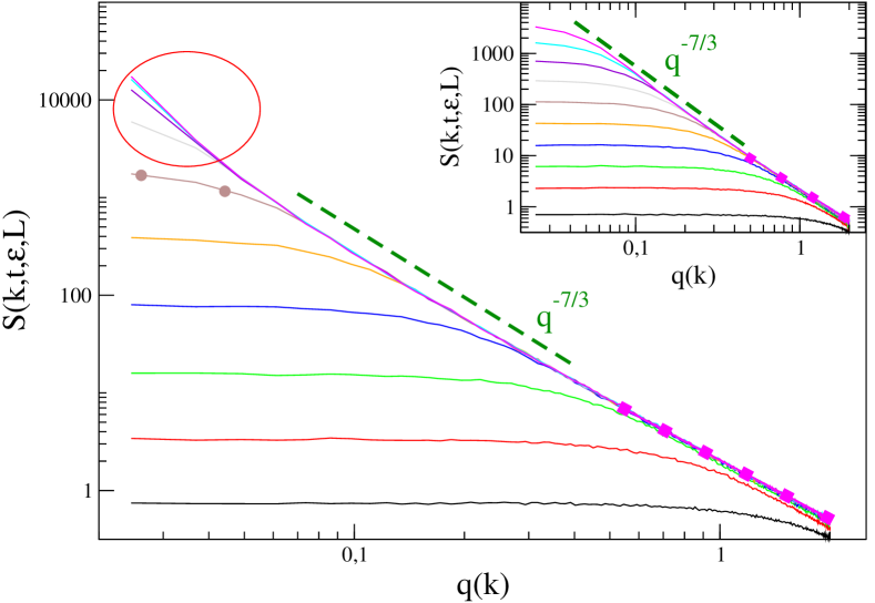
In order to restrict the analysis to the $q$-region where condition Eq. (12) holds we proceed as for the pure case by plotting the data for different times similarly to what done in the main part of Fig. (2), as it is illustrated in Fig. 5 for the RBIM. Then, by considering for example the intermediate time $t=7743$ (brown with circles) in the main part of the figure (with $\epsilon=0.3$) and comparing the curve with the one at the previous time ($t=1292$) we conclude that for $t=7743$ one has $\max\left[\xi^{-1},L^{-1}\right]=\xi^{-1}$ and the condition (12) is met at least down to the wave vector $q\simeq 0.1$. Indeed, up to this point the two curves (for $t=7743$ and $t=1292$) superimpose. For very large times ($t\geq 46416$, say) one observes a pattern of behavior similar to the one seen for large times in the pure case, namely an initial upward bending of the curves before flattening again. This is particularly evident in the main part of the figure in a region indicated with a red ellipse. As we will discuss further in Sec. IV.1, the expected value of $\zeta$ for the RBIM is $\zeta=2/3$ implying $S\simeq q^{-7/3}$ for $q\gg\xi^{-1}$ in an infinite system. On the contrary, we see that at least for $t\geq 46416$ the curves reach a larger slope before flattening again. As in the pure case this feature identify quite clearly the fact that $\max\left[\xi^{-1},L^{-1}\right]=L^{-1}$, finite size effects become relevant and condition (12) is spoiled. Notice that this occurs around the same wave vector $q\simeq 0.05$ of the pure case. Interestingly, by repeating the analysis for $\epsilon=1$ (data in the inset of Fig. 5) we find that finite size effects are much smaller with respect to the case with $\epsilon=0.3$: Only for the longest time $t=10^{7}$ one observes a weak upward bending of the curve. This difference with the case $\epsilon=0.3$ occurs because the larger the disorder is, the slower is the growth of $\xi(t)$, and finite size effects are pushed to larger times.

By repeating the procedure described above both for the RBIM and the RFIM, for any choice of $t$ and of the disorder strength we end up with a definition of the $q$-sector corresponding to the condition (12). This being done, we have purged the data in order to keep only those in the sector where Eq. (12) is fulfilled: these are the only ones which have been plotted in Figs. 3,4. Then, the slope of the curves in these figures gives immediate access to the exponent $\zeta$. We stress however, that the main issue considered in this paper, namely the presence of a rich crossover structure between different roughening regimes, can be read out already in the large-$q$ region, as we will discuss below, where no doubts arise on the fulfillment of the condition in Eq. (12).

The properties of the structure factor and the value of the roughening exponent depend on the nature of quenched disordered, either random bonds or random fields. We will then discuss these two cases separately in the next subsections.

Figure 5: $S(k,t,\epsilon=0,L)$ is plotted against $q$ for the RBIM with $\epsilon=0.3$ and, in the inset, for $\epsilon=1$. Different curves correspond to exponentially increasing times ($t=1,6,36,216,1292,7743,46416,278256,1668101,10^{7}$ from bottom to top). The bold-dotted green line is the power-law $q^{-7/3}$ expected for an infinite system in the limit $t\to\infty$. The regions encircled by a red ellipse is the one where finite-size effects show-up. The heavy-dotted magenta line is the power-law $q^{-2}$ expected for small $x$ according to Eq. (8).

IV.1 Random bonds

In the RBIM disorder is only effective on the interfacial spins. Indeed the contribution to the energy of spins away from the interface is independent of the sign of the bulk-phase as long as this phase is uniform (namely all the spins in the bulk are aligned). This is the case with our simulations, since bulk fluctuations are suppressed in the $J_{0}\to\infty$ limit considered here.

When disorder is effective only on the interface the roughening exponent is known to be $\zeta=2/3$ natterman ; dueterzi . This value can be understood on the basis of the following simple scaling argument: The roughness of a piece of interface of linear size $\xi$ is $w\sim\xi^{\zeta}$. The elastic energy associated to this deformation is $E_{el}\sim\xi\cdot(\nabla)^{2}$, where $\nabla\sim\frac{w}{\xi}\sim\xi^{\zeta-1}$ is the (average) local slope of the interface with respect to the flat configuration. Hence $E_{el}\sim\xi^{2\zeta-1}$. Next we want to evaluate the pinning energy associated to the random bonds $E_{pin}=\sum_{ij\in{\cal I}}J_{ij}$, where the sum runs over the bonds located on the actual position of the interface ${\cal I}$. In writing this expression we have used the fact that disorder in this model is only effective around the interface, which has the dimension of a length. Making the identification of this length with $w$ and invoking the central limit theorem we have $E_{pin}\sim\sqrt{w}$. Balancing the two energetic contributions, $E_{el}\simeq E_{pin}$ one obtains $\zeta=2/3$.

This value of the roughening exponent implies, through Eq. (1), a power-law $S\sim q^{-7/3}$ for the structure factor. This agrees with what observed in Fig. 3. Indeed, for sufficiently small wavevectors $q\ll\lambda^{-1}(\epsilon)$, one observes that the pure-like behavior is spoiled, the curves clearly bend upward and the slope of the structure factor increases. Fitting this slope in the range $q\in[0,0.3]$ and extracting the value of the roughness exponent using Eq. (1) we find values between $\zeta=0.60$ and $\zeta=0.71$ ($\zeta=0.60,0.62,0.65,0.66,0.69,0.70,0.71,0.7$ for $\epsilon=0.3,0.4,0.5,0.6,0.7,0.8,0.9,1$, respectively). These values are compatible with the expected exponent $\zeta=2/3$. The smooth crossover from the pure to the disordered behavior and the relatively small range of wavevectors where the disordered behavior is observed do not allow us to provide a more precise determination of the roughness exponent and a clearcut evidence of $\zeta=2/3$, for which we make reference to a specific literature dueterzi . The aim of this paper, however, is not to push simulations to such large sizes and long times to further refine the actual measurement of the roughness exponent for the RBIM, but rather to describe the rich pattern of crossover induced by the presence of disorder, that we will discuss further below. For this task the quality of the data presented here is by far sufficient.

IV.2 Random fields

In the RFIM, disorder not only acts on the interface but also in the bulk ${\cal B}$. Indeed, given a configuration of the quenched random field, the energy of an ordered domain depends on the sign of the magnetization, because an excess of, say, positive random fields favors spins ordering up. In this situation, when disorder couples to the bulk, the roughening exponent is known to be $\zeta=1$ natterman ; nota . Also this value can be understood in terms of the simple scaling argument presented in Sec. IV.1. For the RFIM one has $E_{pin}\sim E_{\cal I}+E_{\cal B}$, where the first term $E_{\cal I}=-\sum_{i\in{\cal I}}H_{i}S_{i}$ is the pinning energy due to the sites around the interface whereas the second one $E_{\cal B}=-\sum_{i\not\in{\cal I}}H_{i}S_{i}$ is the pinning energy due to the bulk. In the thermodynamic limit $E_{\cal B}$, which takes contributions over a surface of order $\xi^{2}$, dominates. Invoking again the central limit theorem and balancing the elastic and the pinning energies one finds $\zeta=1$.

The data of Fig. 4 when the strength of the random field is in the range $\epsilon\lesssim 0.2$ show that the slope of the structure factor, starting from the pure-like behavior $S\sim q^{-2}$ for large $q$, increases up to a value which is consistent with $S(k,t,\epsilon,L)\sim q^{-3}$ (shown with a dot-dashed indigo line) for sufficiently small wavevectors. Recalling Eq. (1) this implies that $\zeta$ is consistent with the expected value $\zeta=1$. Indeed, by fitting the slope of $S$ over the last four points and extracting $\zeta$ we find $\zeta=0.93,1.01,1.05$ for $\epsilon=0.05,0.1,0.2$, respectively.

Let us now move the attention to the large values of $\epsilon$. Starting our analysis from the cases $\epsilon\geq 1$ one can notice that, as already remarked in Sec. IV, the pure-like behavior is never observed. Indeed already at the largest wavevectors the slope of the structure factor is much larger than that $S\sim q^{-2}$ of a pure system. This is better shown in the inset of Fig. 4 where the effective value of $\zeta$ obtained by fitting the slope of $S$ in the range $q\geq 1$ is shown for any value of $\epsilon$. One sees that $\zeta$ saturates for large $\epsilon$ to a value very well consistent with $\zeta=2/3$ (specifically one has $\zeta=0.63$, $\zeta=0.67$, $\zeta=0.66$ for $\epsilon=1,2,3$ respectively), namely the value expected for a system – like the RBIM – where disorder acts only on the interface. This unexpected fact, which represents the main new result of this paper, will be discussed and interpreted later.

Starting from this large-$q$ value, the slope of $S$ (still considering data for $\epsilon\geq 1$) gradually increases as $q$ lowers. For instance, upon fitting the four points with the smallest $q$’s for $\epsilon=1$ one obtains a value yielding an (effective) roughness $\zeta=0.72$. This value,however, is not settled and keeps increasing, consistently with the expectation that $\zeta=1$ is the true asymptotic behavior. With $\epsilon\geq 1$ this cannot be checked further because the curves end around $q\simeq 0.2$, but, for smaller $\epsilon$, the data extend to smaller values of $q$ and a fit over the four smallest $q$ points for $\epsilon=0.8,0.6,0.4,0.3$ yields $\zeta=0.72,0.81,0.93,0.94,0.98$ respectively. This confirms that the true asymptotic regime with $\zeta=1$ is always approached, for any $\epsilon$, if sufficiently small wavevectors are considered.

The pattern of behavior observed in Fig. 4 can be interpreted as follows: in the RFIM the disorder acts both on the interface and in the bulk. The latter is bound to prevail in the limit of large lenghscales and rules the behavior of $S$ at small $q$. However, on small distances, the interface contribution can compete with the bulk one affecting the large-$q$ behavior of $S$. This would explain why the value $\zeta=2/3$ is observed in Fig. 4 for large $q$ when $\epsilon$ is large.

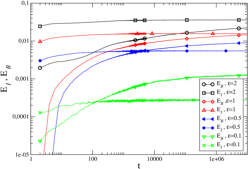
In order to substantiate this conjecture, we have separately computed the energy $E_{\cal I}(t)$ and $E_{\cal B}(t)$ associated to the random fields acting on the surface ${\cal I}$ or in the bulk ${\cal B}$. As it can be seen in Fig. 6, $E_{\cal I}$ dominates over $E_{\cal B}$ for a certain time, before being overtaken by the latter at the crossing time $t^{*}$, when $E_{\cal I}(t^{*})\simeq E_{\cal B}(t^{*})$. Notice that $t^{*}$ increases very fast with the strength of the disorder: for $\epsilon=0.1$ the bulk contribution overwhelms the surface one very soon ($t^{*}\simeq 200$) but for $\epsilon=1$ it is already of the order of the largest simulated time $t=10^{7}$ and goes well beyond this value for $\epsilon=2$.

One can argue that the behavior of global quantities – namely those which are obtained by summing up the contributions from all wavevectors, such as as the total energy of the system or the roughness $W$ – will resemble that of a system where disorder only acts on the interfaces, as the RBIM, for $t\ll t^{*}$. At $t\simeq t^{*}$ a crossover occurs and, for $t\gg t^{*}$ the expected asymptotic behavior of a system where the bulk contribution prevails, as the RFIM, is observed. Associating a length $\Lambda(\epsilon)=\xi(t^{*})$ to the crossing time $t^{*}$ one can say, equivalently, that the crossover occurs when $\xi(t)\sim\Lambda(\epsilon)$.

Concerning non-global quantities that depend on $q$, as the structure factor, for a given time $t$ one expects to observe the crossover around $q\simeq\Lambda^{-1}$: for $q\gg\Lambda^{-1}$ the typical behavior of a system where disorder only acts on the interface is observed, while the bulk contribution will be manifested for $q\ll\Lambda^{-1}$. This explains the crossover from $S\propto q^{-7/3}$ to $S\propto q^{-3}$ observed in Fig. 4 for large $\epsilon$. Notice that from the data of Fig. 6 one realizes that for $\epsilon=1$ one has $t^{*}\simeq 10^{7}$. Therefore the structure factor with $\epsilon=1$ in Fig. 4, which is computed at $t=10^{7}$ cannot access the region where disorder in the bulk dominates. Indeed the exponent $\zeta=1$ is not observed at any $q$.

It must be stressed that, for large $\epsilon$, a value of $\zeta$ compatible with $\zeta=2/3$ was observed in the region of large wavevectors where any problem related to purging the data from finite-size/finite-times effects is avoided and the analysis is more reliable. Not only this value, but the whole crossover leading from the pure like behavior to the one of a system with disorder acting only around the interfaces is displayed in this $q$-region. Indeed, by fitting $\zeta$ from the curves for all values of $\epsilon$ in the range $q\geq 1$ we get a typical sigmoidal behavior starting from $\zeta=1/2$ and converging to $\zeta\simeq 2/3$, as it is shown in the inset of Fig. 4

The crossover structure discussed insofar, where in a certain range a system with bulk disorder behaves as one where randomness acts only on the domain wall, is the main new result of this paper. Let us stress that ignoring this structure can lead to a wrong determination of the true roughening exponent. For instance, fitting naively the structure factor of Fig. 4 with $\epsilon=1$ could lead to the wrong conclusion that the asymptotic roughening exponent for the RFIM is $\zeta=2/3$ whereas this is only a manifestation of a (long-lasting) preasymptotic behavior associated to the effect of disorder on the interface. Pushing the simulations in order to access smaller wavevectors, one could see the crossover towards the truly asymptotic behavior with $\zeta=1$.

Finally, we remark that the results of this paper can be fully accounted for in simple terms as due to a crossover between the behavior of the system with surface and bulk disorder and does not seem to be related to a so-called anomalous scaling behavior altraref .

Figure 6: $E_{\cal I}$ and $E_{\cal B}$ are plotted as a function of time for the RFIM and different values of $\epsilon$ (see key).

V Conclusions

In this paper we have studied the roughening properties of an interface in a disordered medium by computing the dynamical structure factor $S$ in the two-dimensional RBIM and RFIM. The main difference between the two is represented by the fact that the action of the disorder in the former is limited to the interface while in the second it acts also in the bulk. Accordingly, their interfaces belong to different universality classes characterized by the roughening exponents $\zeta=2/3$ and $\zeta=1$, respectively.

Our simulations show a rich behavior of $S$ which can be interpreted as due to crossover phenomena. For both kinds of disorder a first crossover is observed around a certain wavevector $q\simeq\lambda^{-1}(\epsilon)$, where $\lambda(\epsilon)$ is a typical size below which disorder is ineffective, between the behavior of a pure system – for $q>\lambda^{-1}$ – and that of a disordered one for $q<\lambda^{-1}$. In the region where disorder is active one recovers the expected roughness exponent $\zeta=2/3$ when the disorder acts only on the interfaces, as for the RBIM. The behavior is richer when disorder acts also in the bulk, as in the RFIM, with the presence of an additional crossover at a certain wavevector $q\simeq\Lambda^{-1}(\epsilon)<\lambda^{-1}(\epsilon)$ between a region – for $\lambda^{-1}<q<\Lambda^{-1}$ – where the effects of the disorder on the interface prevails, yielding an (effective) exponent $\zeta=2/3$, and the small-$q$ sector where bulk effects are important and the (true) roughening exponent $\zeta=1$ is observed. For this reason the numerical determination of the asymptotic value of $\zeta$ can be, depending on the values of $\lambda$ and $\Lambda$, hindered by the preasymptotic surface effects.

The pattern of crossovers observed in this paper for the RBIM and the RFIM are expected to be representative of a large class of systems where disorder acts prevalently on the interfaces or in the bulk as well.

Acknowledgments F.Corberi acknowledges financial support by MURST PRIN 2010HXAW77_005.

We warmly thank A.B. Kolton for discussions and suggestions.

Appendix A Discussion of the finite-size effects

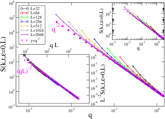
In this section we present a study of the finite-size effects observed in the model discussed in the paper. Fig. 7 shows the behavior of the structure factor for the pure system of different sizes $L$ at a very large time $t=10^{6}$. For the pure case such time is well beyond the equilibration time of the interface, therefore by increasing further $t$ one shouldn’t see any modification to the pattern of Fig. 7. In this figure one observes that the curves follow the behavior $q^{-2}$ expected for an infinite system down to a certain $L$-dependent wavevector below which they bend upward, as already discussed in the paper. The wavevector where this happens decreases as $L^{-1}$ when the system size increases, signalling that this effect is due to the finite-size of the system. A more quantitative test can be done by trying to rescale the data, according to Eq. (9), by plotting $L^{-2}S$ against $qL$. This results in an excellent data collapse, confirming the finite-size nature of the upward bending of the curves. Notice that, as it is shown in the upper inset of Fig. 7, the same phenomenon is observed also by using the different geometry considered in sugref1 . This amounts to tilt the lattice by $45^{o}$, seeding the initial interface vertically in the middle of the system and applying periodic and antiperiodic boundary conditions in the horizontal and vertical directions, respectively. The data in the inset are characterized by the same upward-bending finite-size effect of the main part of the figure, signaling that this is not peculiar to our choice of the boundary conditions. Furthermore, we mention the fact that a similar upward bending due to finite size effects is also observed, in the different context of unisotropic roughening in 2+1 dimension, in vivo .

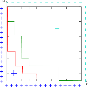
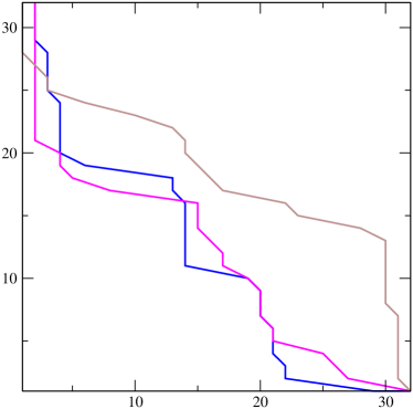
It must be noticed that a similar feature is not observed in continuum theories for interface roughening upton where, instead, the curves for finite $L$ depart from the $k^{-2}$ behavior from below flattening to a finite value. This is due to the different way in which the finite-size is incorporated in the discrete models considered insofar. One can be understand this with the help of Fig. 8, where in the left panel two possible configurations of the interface at the same large time are pictorially sketched. Spins on the left of the interface are down and the other are up; the boundary conditions adopted are also represented. The roughness of the rightmost red interface, denoted hereafter by ${\cal R}$, is somewhat larger than the one of the leftmost green configuration ${\cal G}$. Due to the proximity to the boundary, ${\cal R}$ is characterized by long flat parts, longer than in ${\cal G}$. Such straight segments are actually observed in the real large time dynamics of the model interface as it is shown in the right panel. We can say, therefore, that configurations of the interface with larger roughness are associated to an excess of flat parts due to the boundary condition. With our spin-flip kinetic rule the time needed to change a configuration is proportional to the number of spins that can be updated, namely those on the corners of the interface. An abundance of straight parts reduces the number of such updates and makes the corresponding configuration more long-lived with respect to the ones with many corners. As a consequence, configurations reaching the border exhibit a larger $W$ and, at the same time, they are flatter and live longer, thus providing an extra contribution to the structure factor on the corresponding (small) wavevectors. This explains why, in the presence of finite-size effects, the structure factor exceeds the infinite-size behavior ($S\propto q^{-2}$) and the curves for $S$ bend upward at small wavevectors.

Figure 7: $S(k,t,\epsilon=0,L)$ is plotted against $q$ for the pure case, at a very large time $t=10^{6}$, for different system syzes $L$ (see key). The bold-dotted magenta line is the power-law expected for an infinite system in the limit $t\to\infty$. In the upper inset the same plot is made for a system with a different geometry (see text). In the lower inset the data of the main figure are collapsed by plotting $L^{-2}S(k,t,\epsilon=0,L)$ against $qL$.

Figure 8: Left panel. The position of the interface at time $t=0$ (blue curve on the left) and its evolution at a later time $t$ (red curve on the right) are pictorially sketched. Right panel: real configurations of the model interface in a pure system of size $L=32$ at large times.

References

- (1) T. Vicsek, Fractal Growth Phenomena 2nd ed. (World Scientific, Singapore, 1992). A-L. Barabàsi and H.E. Stanley, Fractal Concepts in Surface Growth, Cambridge: Cambridge University Press (1995).
- (2) M. Nicodemi and H. J. Jensen, Phys. Rev. B 65, 144517 (2002). G. Schehr and P. Le Doussal, Phys. Rev. Lett. 93, 217201 (2004). S. Bustingorry, L. F. Cugliandolo, and D. Dominguez, Phys. Rev. Lett. 96, 027001 (2006). M. Pleimling and U. C. Täuber, Phys. Rev. B 84, 174509 (2011).
- (3) D.A. Huse and C.L. Henley, Phys. Rev. Lett. 54, 2708 (1985). J. Villain, Phys. Rev. Lett. 52, 1543 (1984). M. Kardar, Phys.Rev.Lett. 55, 2923 (1985). D. A. Huse, C. L. Henley, and D. S. Fisher, Phys.Rev.Lett. 55, 2924 (1985).
- (4) G. Blatter, M. V. Feigel’man, V. B. Geshkenbein, A. I. Larkin, and V. M. Vinokur, Rev. Mod. Phys. 66, 1125 (1994).
- (5) D. R. Nelson and V. M. Vinokur, Phys. Rev. B 48, 13060 (1993).
- (6) F. Family and T. Vicsek: J. Phys. A: Math. Gen. 18, 75 (1985). A.B. Kolton, A. Rosso and T. Giamarchi, Phys. Rev. Lett. 95, 180604 (2005).
- (7) F. Corberi, Compt. Ren. Phys. 16, 332 (2015).
- (8) T. Nattermann Europhys. Lett. 4, 1241 (1987). M.E. Fisher, J. Chem. Soc., Faraday Trans. 82, 1569 (1986). M. Kardar, J. Appl. Phys. 61, 3601 (1987). T. Halpin-Healy, Phys. Rev. Lett. 62, 442 (1989); Phys. Rev. A 42, 711 (1990).
- (9) D. A. Huse and C. L. Henley, Phys. Rev. Lett. 54, 2708 (1985); M. Kardar, ibid. 55, 2923 (1985); D. A. Huse, C. L. Henley, and D. S. Fisher, ibid. 55, 2924 (1985).
- (10) N.J. Zhou, B. Zheng and Y.Y. He, Phys. Rev. B 80, 134425 (2009).
- (11) X.P. Qin, B. Zheng and N.J. Zhou, J. Phys. A: Math. Theor. 45, 115001 (2012).
- (12) D. B. Abraham and P. J. Upton, Phys. Rev. B 39, 736 (1989).
- (13) F. Corberi, E. Lippiello, A. Mukherjee, S. Puri and M. Zannetti, Phys. Rev. E 88, 042129 (2013).
- (14) F. Corberi, E. Lippiello, A. Mukherjee, S. Puri and M. Zannetti, J. Stat. Mech.: Theory and Experiment P03016 (2011). F. Corberi, E. Lippiello, M. Zannetti, R. Burioni and A. Vezzani, Phys. Rev. E 91, 062122 (2015).
- (15) F. Corberi, A. de Candia, E. Lippiello and M. Zannetti, Phys. Rev. E 65, 046114 (2002). F. Corberi, E. Lippiello, A. Mukherjee, S. Puri and M. Zannetti Phys. Rev. E 85, 021141 (2012).
- (16) In ref. seppala a value of larger than was also reported.
- (17) E.T. Seppälä, V. Petäjä and M.J. Alava, Phys. Rev.E 58, R5217(R) (1998).
- (18) Y.J. Chen, Y. Nagamine, T. Yamaguchi, and K. Yoshikawa, Phys. Rev. E 82, 021604 (2010).
- (19) E. Vivo, M. Nicoli, and R. Cuerno, Phys. Rev. E 86, 051611 (2012).