Multifractality at non-Anderson disorder-driven transitions
in Weyl semimetals and other systems

Abstract

Systems with the power-law quasiparticle dispersion $\epsilon_{\bf k}\propto k^{\alpha}$ exhibit non-Anderson disorder-driven transitions in dimensions $d>2\alpha$, as exemplified by Weyl semimetals, 1D and 2D arrays of ultracold ions with long-range interactions, quantum kicked rotors and semiconductor models in high dimensions. We study the wavefunction structure in such systems and demonstrate that at these transitions they exhibit fractal behaviour with an infinite set of multifractal exponents. The multifractality persists even when the wavefunction localisation is forbidden by symmetry or topology and occurs as a result of elastic scattering between all momentum states in the band on length scales shorter than the mean free path. We calculate explicitly the multifractal spectra in semiconductors and Weyl semimetals using one-loop and two-loop renormalisation-group approaches slightly above the marginal dimension $d=2\alpha$.

After half a century of studies, disorder-driven transitions in conducting materials still motivate extensive research efforts. Anderson localisation (AL) transition is responsible for turning a metal into an insulator when increasing the disorder strength in dimensions $d\geq 2$ and was believed for several decades to be the only possible disorder-driven transition in non-interacting systems. AL continues to fascinate researchers by its peculiar and universal properties, such as, e.g., multifractality– fractal behaviour of the wavefunctions at the transition with an infinite set of multifractal exponentsEfetov (1999); Evers and Mirlin (2008). Syzranov et al. (2015a, b); Suslov (1994)

A broad class of systems with the power-law quasiparticle dispersion $\epsilon_{\bf k}\propto k^{\alpha}$ in dimensions $d>2\alpha$ displays, however, another single-particle disorder-driven transition distinct from ALSyzranov et al. (2015a, b). This transition, unlike AL, occurs only near a band edge or at a nodal point (in a semimetal). It reflects in the critical behaviour of the disorder-averaged density of states (in contrast with AL), as well as in other physical observables, e.g., conductivity.

Such a transition has first been proposedFradkin (1986a, b) for the specific case of Dirac semimetals ($\alpha=1$, $d=3$) and has recently sparked vigorous studiesShindou and Murakami (2009); Ryu and Nomura (2012); Goswami and Chakravarty (2011); Kobayashi et al. (2014); Ominato and Koshino (2014)Syzranov et al. (2015a, b) Sbierski et al. (2014); Pixley et al. (2015, 2016a); Liu et al. (2016); Sbierski et al. (2015); Shapourian and Hughes (2016); Bera et al. (2016); Syzranov et al. (2016a); Pixley et al. (2016b) of its critical properties in 3D Weyl and Dirac systemsHuang et al. (2015); Xu et al. (2015); Lv et al. (2015). Other playgrounds for the observation of this non-Anderson disorder-driven transition are 1D and 2D arrays of trapped ultracold ions with long-range interactionsGärttner et al. (2015), quantum kicked rotorsSyzranov et al. (2015b) (mappable onto high-dimensional semiconductors), and numerical simulations of Schroedinger equation in $d\geq 5$ dimensionsMarkos (2006); Garcia-Garcia and Cuevas (2007); Ueoka and Slevin (2014); Zharekeshev and Kramer (1998).

Despite these comprehensive studies, the wavefunction structure at these non-Anderson disorder-driven transitions is rather poorly understood. Such transitions are not necessarily accompanied by localisation; they can occur between two phases of localised states [like in 1D (non-chiral) chains of trapped ionsGärttner et al. (2015)] or between two phases of delocalised states [e.g., in single-node Weyl semimetals (WSMs)] or between localised and delocalised states (in a high-dimensional semiconductorSyzranov et al. (2015b)). Particle wavefunctions in all of these cases are characterised by a correlation length that diverges from both sides of the transition.

Results. In this paper we study microscopically wavefunctions $\psi({\bf r})$ at the non-Anderson disorder-driven transitions and demonstrate their multifractal nature. When delocalised states are allowed by symmetry, dimensions, and topology, the typical wavefunctions at the critical disorder strength have a fractal structure and are characterised by a universal non-linear multifractal spectrum $\Delta_{q}$, definedEvers and Mirlin (2008); Efetov (1999) by the inverse participation ratios (IPRs)

$$P_{q}=\int|\psi({\bf r})|^{2q}d{\bf r}\propto L^{-d(q-1)-\Delta_{q}}$$ (1)

in the limit of an infinite system size $L\rightarrow\infty$. Such multifractal behaviour persists even if the wavefunctions are delocalised on both sides of the transition (like in a single-node WSM). Unlike the AL transition, here the multifractal spectrum $\Delta_{q}$ is determined by the elastic scattering on length scales shorter than the mean free path. In systems that allow for localised states near the transition, these states scale as $\int|\psi({\bf r})|^{2q}d{\bf r}\propto\xi^{-d(q-1)-\Delta_{q}}$ when approaching it, where $\xi$ is the localisation length divergent at the transition. In this paper we also calculate the multifractal spectrum $\Delta_{q}$ explicitly for several systems.

We find the multifractal spectrum of a disordered system with the power-law quasipatricle dispersion $\epsilon_{\bf k}=a|{\bf k}|^{\alpha}$ in dimensions $d>2\alpha$ in the orthogonal symmetry class, in the expansion in powers of $\varepsilon$, to be

$$\Delta_{q}^{\text{Semicond}}=\frac{1}{2}\varepsilon q(q-1)+{\cal O}(\varepsilon^{2}),$$ (2)

where $\varepsilon=2\alpha-d$ (and $\varepsilon<0$).

For Weyl semimetals, $\epsilon_{\bf k}=\hat{\bm{\sigma}}{\bf k}$, in $d=2-\varepsilon$ dimensions

$$\Delta_{q}^{\text{WSM}}=-\frac{3}{8}\varepsilon^{2}q(q-1)+{\cal O}(\varepsilon^{3}).$$ (3)

We note that on sufficiently short length scales the multifractality in a Weyl semimetal is similar (with $\varepsilon$ replaced by the dimensionless disorder strength) to that of 2D Dirac fermions on the surfaces of a 3D topological insulator, studied in Ref. Foster (2012). Although there is no phase transition in such 2D systems, their wavefunctions display non-universal short-length multifractal behaviourFoster (2012); Chou and Foster (2014), in contrast with the universal multifractality (3) that persists at all length scales.

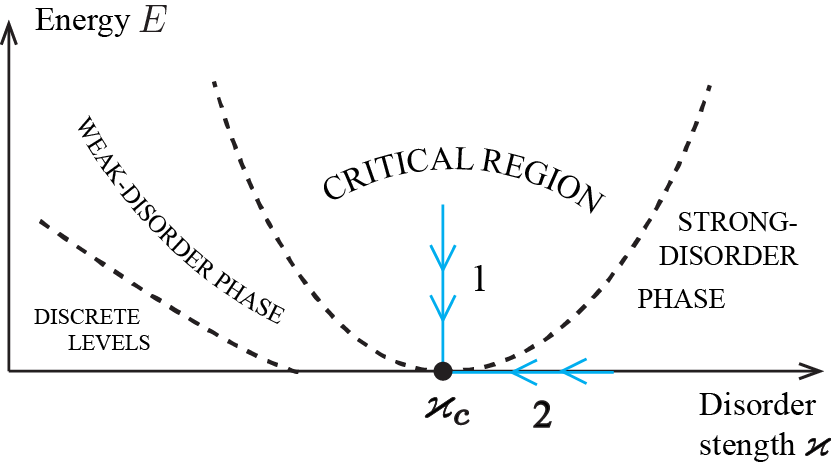
Figure 1: (Colour online) Phase diagram of a finite-size system (with $|\varepsilon|\gtrsim 1$) near a non-Anderson disorder-driven transition. The transition occurs at the energy $E=0$ near the (renormalisedSyzranov et al. (2015b)) band edge or near a nodal point (for semimetals).

The phase diagram of a finite-size system near a non-Anderson disorder-driven transition is shown in Fig. 1. In what follows we measure all energies from a nodal point or a (renormalisedSyzranov et al. (2015b)) band edge[45] set to $E=0$.

For disorder strengths weaker than a critical value (“weak-disorder phase” in Fig. 1), $\varkappa<\varkappa_{c}$, the disorder is perturbatively irrelevantSyzranov et al. (2015a, b) with the dimensionless disorder strength $\gamma(E)\sim[\tau(E)E]^{-1}$ vanishing at small energies $E\rightarrow 0$, where $\tau(E)$ is the elastic scattering time.

Unlike the case of low dimensions, the lowest-energy levels of a sufficiently large high-dimensional system are discrete for $\varkappa<\varkappa_{c}$, as the “level width” $\tau(E)^{-1}$ vanishes faster than the spatial-quantisation gaps $\sim E\propto L^{-\alpha}$ between the lowest levels at $E\rightarrow 0$. The interplay of the level discreteness with multifractality will be discussed below.

For supercritical disorder strength, $\varkappa>\varkappa_{c}$, the dimensionless disorder strength grows at low energies, until reaching the value $\gamma\sim 1$ that marks the boundary of the “strong-disorder phase” (that for $d>2$-dimensional semiconductors in the orthogonal symmetry class also matches the mobility threshold) in Fig. 1.

Inverse participation ratios. The wavefunction structure at energy $E$ and disorder strength $\varkappa$ is conveniently characterised by the disorder-averaged IPRsWegner (1980); Evers and Mirlin (2008); Mirlin (2000)

$$P_{q}(E,\varkappa)=\frac{\left<\sum_{n}\int|\psi_{n}({\bf r})|^{2q}d{\bf r}\>\delta(E-E_{n})\right>_{\text{dis}}}{\left<\sum_{n}\delta(E-E_{n})\right>_{\text{dis}}}\equiv$$

$$\frac{i^{q-2}}{2\pi\rho(E)}\lim_{\eta\rightarrow 0}(2\eta)^{q-1}\left<\left[G_{R}({\bf r},{\bf r},E,\eta)\right]^{q-1}G_{A}({\bf r},{\bf r},E,\eta)\right>_{\text{dis}},$$ (4)

where $G_{R,A}({\bf r},{\bf r}^{\prime},E,\eta)=\sum_{n}\frac{\psi_{n}^{*}({\bf r})\psi_{n}({\bf r})}{E-E_{n}\pm i\eta}$ are the retarded and advanced Green’s functions with an artificially introduced “dephasing rate” $\eta$, $E_{n}$ are the energies of the eigenstates $\psi_{n}$ for a given disorder realisation, and $\rho(E)$ is the (disorder-averaged) density of states.

Below we compute the disorder-averaged IPRs (4) near the critical point $(E=0,\varkappa=\varkappa_{c})$ as a function of the system size $L$ or the localisation length $\xi$. The IPRs, Eq. (4), are mimicked by the diagram in Fig. 2a.

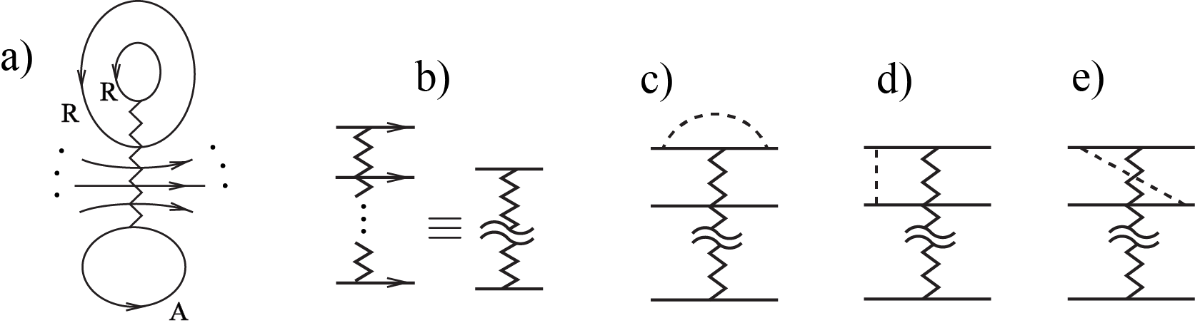
Figure 2: Diagrams for calculating the IPR. a) Product of $q$ Green’s functions before disorder averaging, cf. Eq. (4). b) Vertex that connects $q$ Green’s functions. c)-e) Diagrams for the one-loop renormalisation of the vertex. For $\epsilon_{\bf k}\propto|{\bf k}|^{\alpha}$, diagrams c)-e) have equal values. In Weyl semimetals and other odd-spectrum ($\epsilon_{\bf k}=-\epsilon_{-{\bf k}}$) systems diagrams d) and e) cancel each other.

Unlike the case of low dimensions, $d<2\alpha$, the low-energy properties of high-dimensional materials under consideration are affected by elastic scattering between all momenta in the bandSyzranov et al. (2015b). Such ultraviolet processes are qualitatively important on length scales shorter than the mean free path $\ell$, and, in particular, determine the criticality and multifractality near the transition point due to the diverging $\ell$. This leads to the critical properties and multifractal spectrum different from those at the usual AL transition, that occurs for states away from nodes and band edges and is described by non-linear sigma-modelsEfetov (1999) on length scales longer than the mean free path.

Renormalisation procedure. The effects of the ultraviolet scattering can be addressed in a controlled way by means of a perturbative renormalisation-group (RG) controlled by the small parameterGoswami and Chakravarty (2011)Syzranov et al. (2015a, b) Pixley et al. (2016a); Syzranov et al. (2016a) $\varepsilon=2\alpha-d$. The results obtained from this approach are expected to hold qualitatively also in systems with $|\varepsilon|\gtrsim 1$.

To perform renormalisations, we rewrite the disorder-averaged IPRs using a supersymmetricEfetov (1999) field theory:

$$P_{q}= \lim_{\eta\rightarrow 0}\frac{(2\eta)^{q-1}}{2\pi\rho(E)}V(K)\int{\cal D}\psi{\cal D}\psi^{\dagger}\left[s_{R}({\bf r})s_{R}^{*}({\bf r})\right]^{q-1}$$

$$s_{A}({\bf r})s_{A}^{*}({\bf r})\>\exp({-{\cal L}_{0}-{\cal L}_{\text{int}}}),$$ (5a)

$${\cal L}_{0}= -i\int\psi^{\dagger}\Lambda^{\frac{1}{2}}\left[E\,\lambda(K)+i\eta\Lambda\lambda(K)-\epsilon_{\hat{\bf k}}\right]\Lambda^{\frac{1}{2}}\psi\,d{\bf r},$$ (5b)

$${\cal L}_{\text{int}} =\frac{1}{2}\varkappa(K)\int(\psi^{\dagger}\Lambda\psi)^{2}d\,{\bf r},$$ (5c)

where $\psi^{\dagger}$ and $\psi$ are $4$-component supervectors in the $FB\otimes RA$ (fermion-boson $\otimes$ retarded-advanced) space, $s$ and $s^{*}$ are the bosonic components of the supervectors, and $\Lambda=\left(\sigma_{z}\right)_{RA}\otimes\mathds{1}_{FB}$. The factors with $\Lambda$-matrices in Eq. (5b) ensure the convergence of the supersymmetric integral with respect to the bosonic variablesMirlin (2000).

Upon repeatedly integrating out shells of highest momenta, the action (5b)-(5c) reproduces itself with renormalised disorder strength $\varkappa(K)$ and the parameters $\lambda(K)$ and $V(K)$ that “flow” with the running cutoff $K$ and initial values $\varkappa(K_{0})=\varkappa_{0}$, $\lambda(K)=1$, and $V(K)=1$, where $K_{0}$ is the ultraviolet momentum cutoff set by the bandwidth or the impurity sizeSyzranov et al. (2015b).

The parameters $\lambda$ and $V$ grow upon coarse-graining and exhibit singular behaviour with

$$V\propto\lambda^{\zeta}$$ (6)

at the critical disorder, $\varkappa=\varkappa_{c}$. The IPRs (4) can be rewritten as

$$P_{q}(E,\varkappa_{0},K_{0})=\lambda^{\zeta-q}P_{q}[\lambda(K)E,\varkappa(K),K],$$ (7)

where $P_{q}[\lambda(K)E,\varkappa(K),K]$ is the IPR of an effective renormalised system with the same quasiparticle dispersion $\epsilon_{\bf k}\propto k^{\alpha}$, but with renormalised disorder strength $\varkappa$ and energy $\lambda E$ and that excludes scattering into momentum states $k>K$ that were removed by the RG procedure.

The RG has to be stopped either when the spatial quantisation effects become important or if it runs into the regime of strong disorder, $\varkappa K^{-\varepsilon}\sim 1$. The renormalised system is then equivalent to a simple (low-dimensional) system with discrete energy levels or with a constant density of states and unaffected by scattering into high-momentum modes; the IPR $P_{q}$ of such a system can be found using conventional methods developed for low-dimensional systemsEfetov (1999); Mirlin (2000).

Fractality of delocalised states. In what immediately follows we consider a system with delocalised finite-energy states at $\varkappa=\varkappa_{c}$ [along path $1$ in Fig. (1)], as, e.g., in a $d>\max(2,2\alpha)$-dimensional system with potential disorder.

The RG procedure at critical disorder is terminated when either the momentum $K$ reaches $1/L$ or the spatial quantisation effects become important (i.e. the energy levels become discrete). The renormalised system is then either ballistic (for small $\varepsilon$, that ensures weak disorder at the critical point) or equivalent to a usual weakly disordered metal (for larger $\varepsilon$), withEfetov (1999); Evers and Mirlin (2008) $P_{q}\propto L^{-d(q-1)}$.

The characteristic energy $E_{L}$ of terminating the RG is related to the system size $L$ as $E_{L}\propto L^{-z}$, where $z$ is the dynamical critical exponent. Using that $\lambda(K\sim L^{-1})E_{L}\sim\epsilon_{K\sim L^{-1}}\propto L^{-\alpha}$, we find $\lambda(K\sim L^{-1})\propto L^{z-\alpha}$, which, together with Eq. (7) gives the multifractal spectrum

$$\Delta_{q}=-(\zeta-q)(z-\alpha).$$ (8)

Localised states. For trivial-topology systems in the orthogonal symmetry class the states in the “strong-disorder phase” (Fig. 1) are localised. Also, all states on the phase diagram are localised in systems in $d\leq 2$ dimensions (if allowed by symmetry/topology).

Near the critical point of the non-Anderson disorder-driven transition localised states are still multifractal on length scales shorter than the localisation length $\xi$ (that diverges at the transition).

For zero-energy states at supercritical disorder, $\varkappa>\varkappa_{c}$, (along path 2 in Fig. 1) the RG is stopped when reaching strong disorder, $\varkappa(K)K^{-\varepsilon}\sim 1$. Such $E=0$-states are then characterised by only one length scale $K^{-1}$ that gives the localisation length $\xi$. Similarly to the case of delocalised states in a size-$L$ system, we find that $\lambda(K\lesssim\xi^{-1})\propto\xi^{z-\alpha}$, and the participation ratio

$$P_{q}\propto\xi^{-d(q-1)-\Delta_{q}}$$ (9)

with the multifractal spectrum (8). The non-trivial scaling of the IPR (9) with the size of the localisation cell reflects the multifractality of the wavefunctions on length scales $L<\xi$.

Orthogonal semiconductors. For a disordered system with the quasiparticle dispersion $\epsilon_{\bf k}=a|{\bf k}|^{\alpha}$ the RG flow of the system parameters is given in terms of the dimensionless disorder strength $\gamma=4C_{d}\varkappa K^{-\varepsilon}/a^{2}$, with $C_{d}=2^{1-d}\pi^{-\frac{d}{2}}/\Gamma\left(\frac{d}{2}\right)$, by the RG equations

$$\partial_{l}V ={q(2q-1)}V\gamma/4+\ldots,$$ (10a)

$$\partial_{l}\lambda =\gamma\lambda/4+\ldots,$$ (10b)

$$\partial_{l}\gamma =\varepsilon\gamma+\gamma^{2}+\ldots.$$ (10c)

where $l=\ln(K_{0}/K)$ and $\ldots$ are the terms of higher orders in $\gamma$. Eqs. (10b) and (10c) for the renormalisation of the energy and the disorder strength have been obtained previously in Refs. Syzranov et al., 2015a and Syzranov et al., 2015b. Eq. (10a) describes the flow of the preexponential in Eq. (5a).

The renormalisations (10a)-(10c) can be also easily obtained diagrammatically. For instance, the one-loop renormalisation of the vertex $V$, Fig. 2b, is given by $q$ diagrams equivalent to 2c, $q(q-1)$ diagrams equivalent to 2d, and $q(q-1)$ diagrams equivalent to 2e. All these diagrams have the same value for the dispersion under consideration, hence the prefactor $q(2q-1)$ in Eq. (10a). The renormalisation of the disorder strength $\gamma$ and the parameter $\lambda$ for the dispersion under consideration has been described in detail in Ref. Syzranov et al., 2015b.

In the one-loop order we find from Eqs. (10a)-(10c) that $\zeta\approx q(2q-1)$ andSyzranov et al. (2015b) $z\approx\alpha-\varepsilon/4$, which, together with Eq. (8), gives the multifractal spectrum (2).

Chiral systems, such as Weyl semimetals or chiral chains with long-range hoppingGärttner et al. (2015), often have odd quasiparticle spectra, $\epsilon_{\bf k}=-\epsilon_{-{\bf k}}$, which leads to the mutual cancellation of diagrams 2d and 2e. The RG flow of the vertex $V$ is given by Eq. (10a) with the replacement $q(2q-1)\rightarrow 2q$ and with the dimensionless disorder strength $\gamma=2C_{d}K^{-\varepsilon}\varkappa$. The flow of $\lambda$ is given by Eq. (10b) with the replacement $4\rightarrow 2$. From the RG equations we find $\zeta=q+{\cal O}(\varepsilon)$ [cf. Eq. (6)], which, according to Eq. (8), gives vanishing multifractality $\Delta_{q}=0$ in the one-loop order. Thus, finding the multifractal behaviour in such chiral systems requires RG analysis in higher orders.

In what follows we present the result for a Weyl semimetal (see Appendix for a detailed two-loop RG analysis of multifractality using the minimal-subtraction scheme).

Weyl semimetals are 3D systems with the quasiparticle dispersion $\epsilon_{{\bf k}}=\hat{\bm{\sigma}}{\bf k}$, where $\hat{\bm{\sigma}}$ is a vector of Pauli matrices. WSM properties near the non-Anderson disorder-driven transition can be studied by performing RG analysis in $d=2-\varepsilon$ dimensions with setting $\varepsilon=-1$ at the end of the calculation. Although the RG procedure is controlled by small $\varepsilon$, it is knownSbierski et al. (2014); Gärttner et al. (2015); Liu et al. (2016); Pixley et al. (2016a); Bera et al. (2016) to give good agreement with numerical results even for $\varepsilon\sim 1$.

The flows of the parameters of a disordered WSM in $2-\varepsilon$ dimensions are given by (see Appendix)

$$\partial_{l}V =\frac{q}{2}V\gamma+\left(\frac{3}{8}q^{2}-\frac{q}{4}\right)V\gamma^{2}+\ldots,$$ (11a)

$$\partial_{l}\lambda =\frac{1}{2}\lambda\gamma+\frac{1}{8}\lambda\gamma^{2}+\ldots,$$ (11b)

$$\partial_{l}\gamma =\varepsilon\gamma+\gamma^{2}+\frac{1}{2}\gamma^{3}+\ldots.$$ (11c)

Eqs. (11b) and (11c) for the renormalisation of the energy and disorder strength in a disordered WSM have been derived previously in Refs. Schuessler et al., 2009 and Syzranov et al., 2016a and in Refs. Wetzel, 1985; Ludwig, 1987; Luperini and Rossi, 1991; Bondi et al., 1990; Tracas and Vlachos, 1990; Ludwig and Wiese, 2003 for the equivalent Gross-Neveu model. An equation equivalent to Eq. (11a) has also been derived in Ref. Foster (2012) to describe the wavefunctions of 2D Dirac fermions on the surface of a 3D topological insulatorFoster (2012); Chou and Foster (2014).

From Eqs. (11a)-(11c) we find to the two-loop order $\zeta=q-\frac{3}{4}(q^{2}-q)\varepsilon+{\cal O}(\varepsilon^{2})$, which, together with $z=1-\frac{\varepsilon}{2}+\ldots$ and Eq. (8), gives the multifractal spectrum (3).

Level discreteness and observability of multifractality. Observation of multifractality at the critical point ($E=0$, $\varkappa=\varkappa_{c}$) requires that the disorder-averaged energy spectrum of the system at this point is continuous, i.e. smeared by disorder and unaffected by the spatial quantisation. This condition is always met in systems with $|\varepsilon|\sim 1$ as the “level width” $\tau(E_{n})^{-1}\sim E_{n}$ for the lowest levels $n$ is of the order of their energies $E_{n}$.

However, for some systems, e.g., chains of ultracold ionsRicherme et al. (2014), it is possible to realiseGärttner et al. (2015) $|\varepsilon|\ll 1$, that corresponds to weak disorder $\gamma_{c}\sim|\varepsilon|$ at the critical point and the existence of a large number $\sim 1/\varepsilon$ of energy levels that remain discrete [$\tau^{-1}(E_{n})\ll|E_{n}-E_{n-1}|$] at the critical disorder, although the energies and the spacings between these levels vanish in the limit $L\rightarrow\infty$. The multifractal behaviour in such systems is observable only on sufficiently short length scales

$$L<L_{\text{discr}}=L\,|\varepsilon|^{\frac{1}{d}}$$ (12)

that correspond to the wavelengths of higher levels belonging to the continuous part of the energy spectrum.

Rare-region effects. The perturbative RG that we used in this paper neglects non-perturbative instantonic contributions[Suslov, 1994,Syzranov et al., 2015b] to the field theory (5a)-(5c), that, e.g., result in the formation of Lifhsitz tails near band edges and always lead to a finite density of statesWegner (1981); Nandkishore et al. (2014) near nodes. The effects of such instantons on physical observables, such as the density of states and conductivity, are rather small near the critical point in high-dimensional systems and were undetectable in all numerical studiesKobayashi et al. (2014); Sbierski et al. (2014); Pixley et al. (2015, 2016a); Liu et al. (2016); Sbierski et al. (2015); Shapourian and Hughes (2016); Bera et al. (2016) so far except Ref. Pixley et al., 2016b.

Another potential consequence of rare-region (instantonic) effects, albeit currently not demonstrated analytically, may be the “rounding” of the criticality, i.e. preventing the divergence of the correlation length near the critical point, and thus converting the phase transition of the type discussed here into a sharp crossover, with the latter scenario advocated in Ref. Pixley et al., 2016b. In our view, the plausibility of this scenario deserves further investigation, in particular, in systems that disallow localisation by symmetry and topology. In the case the criticality does get smeared in a system, the wavefunction multifractality studied here is observable on distances shorter than a large characteristic length set by the rare-region effects.

Acknowledgements. We are grateful to A.W.W. Ludwig for useful motivating discussions at the initial stages of this work and to P.M. Ostrovsky for previous collaboration. Also, we thank M.S. Foster for valuable discussions. Our work was financially supported by the NSF grants DMR-1001240 (LR and SVS), DMR-1205303(VG and SVS), PHY-1211914 (VG and SVS), PHY-1125844 (SVS) and by the Simons Investigator award of the Simons Foundation (LR).

Appendix A Appendix: Two-loop RG flow in a Weyl semimetal

Here we present a two-loop renormalisation-group analysis of the multifractal properties of a disordered Weyl semimetal in $d=2-\varepsilon$ dimensions using the minimal subtraction schemePeskin and Schroeder (1975).

A similar scheme has been applied recently Syzranov et al. (2016a) to compute the correlation-length and dynamical exponents for a WSM to the two-loop order, following previous studies of grapheneSchuessler et al. (2009) and of the equivalent Gross-Neveu modelWetzel (1985); Ludwig (1987); Luperini and Rossi (1991); Bondi et al. (1990); Tracas and Vlachos (1990); Ludwig and Wiese (2003). Also, a similar multifractality analysis has been carried out in Ref. Foster (2012) for 2D ($\varepsilon=0$) Dirac fermions on the surface of a 3D topological insulator. Although there is no disorder-driven phase transition in such a 2D system, the wavefunctions display multifractal behaviour on sufficiently short length scales.

Renormalisation scheme

For performing two-loop renormalisation-group analysis it is convenient to rewrite the IPRs (4) as a derivative of a partition function with respect to a supersymmetry-breaking term:

$$P_{q}= -\lim_{\eta\rightarrow 0}\frac{(2\eta)^{q-1}}{2\pi\rho(E)}\partial_{V_{0}}Z|_{V_{0}=0}$$ (13a)

$$Z= \int{\cal D}\psi{\cal D}\psi^{\dagger}\>\exp({-{\cal L}_{0}-{\cal L}_{\text{int}}-{\cal L}_{V_{0}}})$$ (13b)

$${\cal L}_{0}= -i\int\psi^{\dagger}\left[i\omega+i\eta\Lambda-\hat{\bm{\sigma}}\hat{\bf k}\right]\psi\,d{\bf r},$$ (13c)

$${\cal L}_{\text{int}}= \frac{1}{2}\varkappa_{0}\int(\psi^{\dagger}\psi)^{2}d\,{\bf r}$$ (13d)

$${\cal L}_{V_{0}}= V_{0}\int\left[s_{R}({\bf r})s_{R}^{*}({\bf r})\right]^{q-1}s_{A}({\bf r})s_{A}^{*}({\bf r})d{\bf r}.$$ (13e)

Here we have introduced a positive Matsubara frequency $\omega>0$ that ensures the convergence of the superintegral (13b) with respect to the bosonic components of the supervectors $\psi$ and $\psi^{\dagger}$ and, in the below calculation, also regularises infrared divergences of momentum integrals in $d=2-\varepsilon$ dimensions for $\varepsilon>0$.

The Lagrangian of the system in the minimal subtraction scheme is separated into the effective Lagrangian ${\cal L}_{E}$ that describes the long-wave behaviour of the physical observables and the counterterm Lagrangian ${\cal L}_{\text{counter}}$ that cancels contributions divergent in the powers of $1/\varepsilon$:

$${\cal L}= {\cal L}_{E}+{\cal L}_{\text{counter}},$$ (14a)

$${\cal L}_{E}= -i\int\Psi^{\dagger}\left[i\Omega+i\eta\lambda\Lambda-\hat{\bm{\sigma}}\hat{\bf k}\right]\Psi\,d{\bf r}$$

$$+\frac{1}{2}\varkappa\int(\Psi^{\dagger}\Psi)^{2}d\,{\bf r}$$ (14b)

$$+V\int\left[S_{R}({\bf r})S_{R}^{*}({\bf r})\right]^{q-1}S_{A}({\bf r})S_{A}^{*}({\bf r})d{\bf r},$$ (14c)

where the velocity of the renormalised Weyl fermions (the coefficient before $\hat{\bm{\sigma}}\hat{\bf k}$) is set to unity, without loss of generality, by appropriately choosing the field $\Psi$. The scale $\Omega>0$ sets the characteristic momentum of the long-wave behaviour. The coefficients $V$ and $V_{0}$ before the source terms (13e) and (14c) are considered infinitesimal in the calculation below.

We note, that in general the renormalisation generates additional terms $\propto V\int\left[S_{R}({\bf r})S_{R}^{*}({\bf r})\right]^{m}S_{A}({\bf r})S_{A}^{*}({\bf r})d{\bf r}$ with $m<q-1$, which we neglect here because their contributions to the partition function (13b) are less singular $\propto\eta^{-(m-1)}$ at $\eta\rightarrow 0$ than that of the term (14c), and, thus, they do not contribute to the IPRs (13a).

The minimal subtraction schemePeskin and Schroeder (1975) consists in calculating perturbative corrections to the Lagrangian (14b) and choosing the counterterms ${\cal L}_{\text{counter}}$ to cancel divergent in powers of $1/\varepsilon$ contributions. The RG equations can then be derived by relating the “observable” parameters $\Psi$, $\Omega$, $\varkappa$, and $V$ to the “bare” ones $\psi$, $\omega$, $\varkappa_{0}$, and $V_{0}$.

All momentum integrals in such a calculation are convergent in low dimensions $d=2-\varepsilon$ with $\varepsilon>0$. The results have to be analytically continued to higher dimensions, $\varepsilon<0$, at the end of the calculation (dimensional regularisation). The “dephasing rate” $\eta$, sent to zero at the end of the calculation [cf. Eqs. (13a) and (13c)], may be assumed to be significantly smaller than the scale $\Omega$ and neglected when computing the parameters of the renormalised Lagrangian.

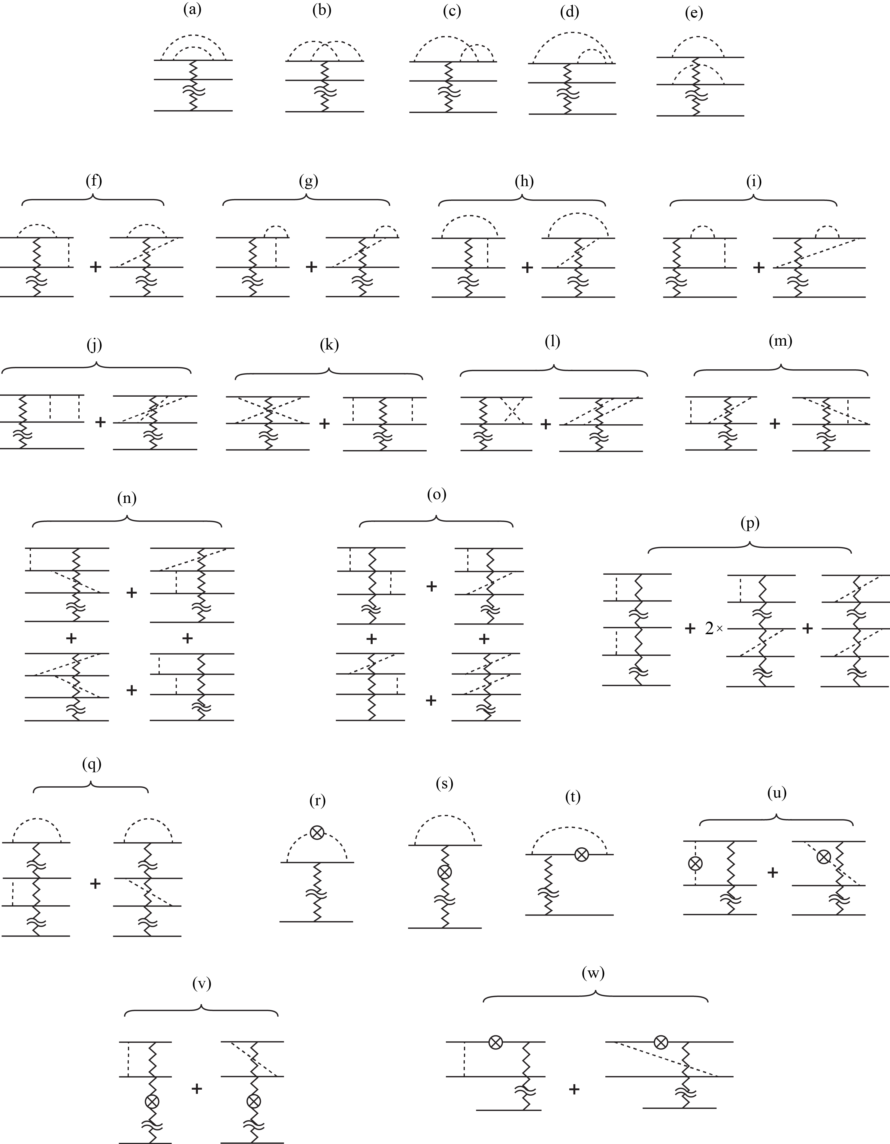
Figure 3: Diagrams for the two-loop renormalisation of the vertex $V$.

One-loop renormalisations

In the one-loop order the renormalisation of the disorder strength $\varkappa$ and the quasiparticle energy $\Omega$ has been considered in detail in Ref. Syzranov et al., 2016a.

The one-loop perturbative correction to the vertex $V$ is described by the diagrams in Fig. 2c-e and the topologically equivalent diagrams. Since the “dephasing rate” $\eta$ may be neglected when considering the respective high-momentum scattering processes, the advanced and retarded Green’s functions may be taken identical $G^{A}({\bf p},i\Omega)=G^{R}({\bf p},i\Omega)=(i\Omega-\hat{\bm{\sigma}}{\bf p})^{-1}$ when evaluating these diagrams. The sum of diagrams 2c-e is given by

$$(\delta V)^{\text{1-Loop}}$$

$$=q(q-1)V\varkappa\int_{\bf p}\frac{1}{i\Omega-\hat{\bm{\sigma}}{\bf p}}\otimes\left(\frac{1}{i\Omega+\hat{\bm{\sigma}}{\bf p}}+\frac{1}{i\Omega-\hat{\bm{\sigma}}{\bf p}}\right)$$

$$+qV\varkappa\int_{\bf p}\frac{1}{(i\Omega-\hat{\bm{\sigma}}{\bf p})^{2}}=-\frac{q}{\varepsilon}\varkappa VC_{2-\varepsilon}\Omega^{-\varepsilon}+{\cal O}(1),$$ (15)

where the prefactors $q(q-1)$ and $q$ account for the numbers of topologically equivalent diagrams, $\int_{\bf p}\ldots=\int d^{d}{\bf p}/(2\pi)^{d}\ldots$, and $C_{d}=2^{1-d}\pi^{-\frac{d}{2}}/\Gamma\left(\frac{d}{2}\right)$, and $\ldots\otimes\ldots$ is the tensor product of the two subspaces of the two $2\times 2$ propagators connected by impurity lines in Figs. 2d and 2e; the structure of the correction is trivial in the other propagators’ subspaces.

The perturbative corrections to the disorder strength $\varkappa$ and the frequency $\Omega$ have been calculated in detail in Ref. Syzranov et al., 2016a. The velocity of the Weyl fermions [the coefficient before the $\hat{\bm{\sigma}}\hat{\bf k}$ term in Eq. (14b)] does not receive first-order corrections.

The singular part $\propto 1/\varepsilon$ of the one-loop corrections to the Lagrangian is cancelled by the counterterms

$${\cal L}_{\text{counter}}^{(1)}= \int\Psi^{\dagger}\>\delta^{(1)}\Omega\>\Psi\,d{\bf r}+\frac{1}{2}\delta^{(1)}\varkappa\int(\Psi^{\dagger}\Psi)^{2}\,d{\bf r}$$

$$+\delta^{(1)}V\int\left[S_{R}({\bf r})S_{R}^{*}({\bf r})\right]^{q-1}S_{A}({\bf r})S_{A}^{*}({\bf r})\,d{\bf r}$$ (16)

with

$$\delta^{(1)}\Omega= -\frac{1}{\varepsilon}\Omega\cdot\varkappa C_{2-\varepsilon}\Omega^{-\varepsilon},$$ (17a)

$$\delta^{(1)}\varkappa= -\frac{2}{\varepsilon}\varkappa^{2}C_{2-\varepsilon}\Omega^{-\varepsilon},$$ (17b)

$$\delta^{(1)}V= -\frac{q}{\varepsilon}V\varkappa C_{2-\varepsilon}\Omega^{-\varepsilon}.$$ (17c)

The presence of the one-loop counterterms (16) requires introducing the respective diagrammatic elements, Fig. 4, in addition to the propagators and impurity lines, when calculating diagrammatically perturbative corrections beyond the one-loop order.

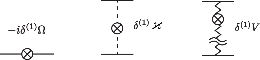
Figure 4: Additional diagrammatic elements that come from the one-loop counterterms.

Two-loop diagrams for the source-term renormalisation

The diagrams that describe the renormalisation of the source term $\propto V$ in the two-loop order are shown in Fig. 3.

Diagrams in Fig. 3(a)-(m) are computed similarly to the two-loop diagrams for the renormalisation of the disorder strength, obtained by replacing the zigzag line by an impurity line and considered in detail in Ref. Syzranov et al., 2016a. The values of diagrams 3(a)-(m), together with the numbers of equivalent diagrams, are provided in Table 1.

Diagrams 3(n)-(p) are regular in $\varepsilon$ due to the mutual cancellation of the singularities coming from blocks with vertical and diagonal impurity lines. For instance, the sum of the diagrams in Fig. 3(n) (see also Fig. 5) can be evaluated (in units $V\varkappa^{2}$) as

$$\int\frac{1}{i\Omega-\hat{\bm{\sigma}}{\bf p}}\frac{1}{i\Omega-\hat{\bm{\sigma}}({\bf p}+{\bf q})}\otimes\left(\frac{1}{i\Omega-\hat{\bm{\sigma}}{\bf q}}+\frac{1}{i\Omega+\hat{\bm{\sigma}}{\bf q}}\right)$$

$$\otimes\left(\frac{1}{i\Omega-\hat{\bm{\sigma}}{\bf p}}+\frac{1}{i\Omega+\hat{\bm{\sigma}}{\bf p}}\right)$$

$$=4\Omega^{2}\int\frac{(i\Omega+\hat{\bm{\sigma}}{\bf p})[i\Omega+\hat{\bm{\sigma}}({\bf p}+{\bf q})]}{(\Omega^{2}+p^{2})^{2}(\Omega^{2}+q^{2})[\Omega^{2}+({\bf p}+{\bf q})^{2}]}$$

$$=4\Omega^{2}\int\frac{(\hat{\bm{\sigma}}{\bf p})(\hat{\bm{\sigma}}{\bf q})}{(\Omega^{2}+p^{2})^{2}(\Omega^{2}+q^{2})[\Omega^{2}+({\bf p}+{\bf q})^{2}]}$$

$$+4\Omega^{2}\int\frac{1}{(\Omega^{2}+p^{2})(\Omega^{2}+q^{2})[\Omega^{2}+({\bf p}+{\bf q})^{2}]}$$

$$-8\Omega^{4}\int\frac{1}{(\Omega^{2}+p^{2})^{2}(\Omega^{2}+q^{2})[\Omega^{2}+({\bf p}+{\bf q})^{2}]}$$

$$={\cal O}(1).$$ (18)

(For detailed calculations of the last integrals see Ref. Syzranov et al., 2016a). The values of diagrams 3(n)-(q) are given in Table 2.

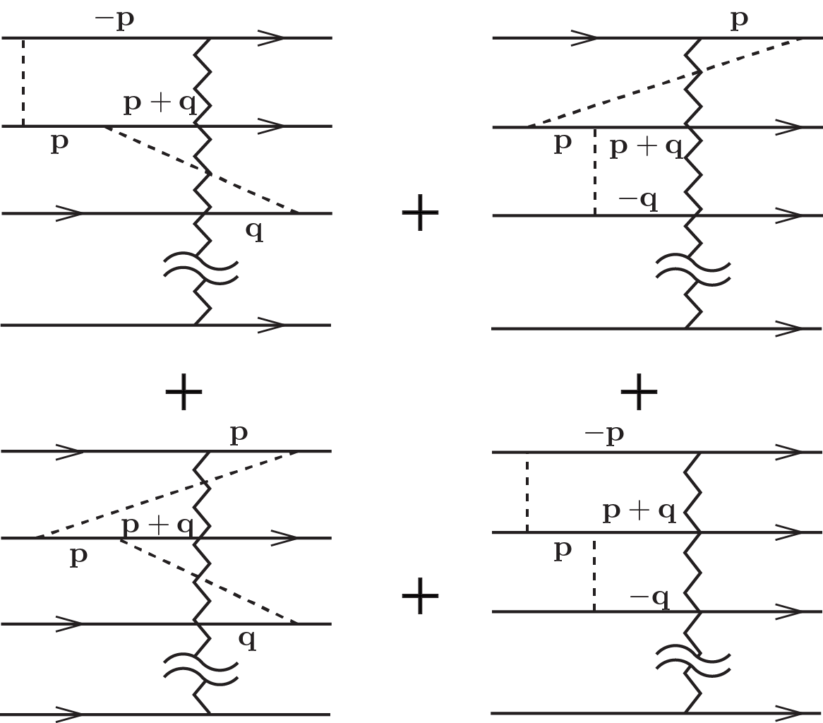
Figure 5: Momenta in diagram (n) in Fig. 3.

Similarly one can show the vanishing of singular in $1/\varepsilon$ contributions in diagrams 3(o) and 3(p).

Diagrams 3(q) are given by (in units $V\varkappa^{2}$)

$$\int_{\bf q}\frac{1}{(i\Omega-\hat{\bm{\sigma}}{\bf q})^{2}}\otimes\int_{\bf p}\frac{1}{i\Omega-\hat{\bm{\sigma}}{\bf p}}$$

$$\otimes\left(\frac{1}{i\Omega-\hat{\bm{\sigma}}{\bf p}}+\frac{1}{i\Omega+\hat{\bm{\sigma}}{\bf p}}\right)$$

$$=-\frac{1}{\varepsilon}\left(C_{2-\varepsilon}\Omega^{-\varepsilon}\right)^{2}+{\cal O}(1)$$ (19)

Diagrams 3(r)-(w) are the two-loop diagrams for the corrections to the vertex $V$ that contain one-loop counterterms and are equivalent to similar diagrams in Ref. Syzranov et al., 2016a, up to replacing the zigzag line or its counterterm by the impurity line or its counterterm, with the values provided in Table 3.

Diagram	# Equivalent diagrams	Value
(a)	$q$	$\frac{1}{\varepsilon^{2}}-\frac{2}{\varepsilon}$
(b)	$q$	$-\frac{1}{2\varepsilon^{2}}+\frac{2}{\varepsilon}$
(c)	$2q$	$\frac{1}{2\varepsilon^{2}}-\frac{1}{\varepsilon}$
(d)	$2q$	$-\frac{1}{2\varepsilon}$
(e)	$\frac{q(q-1)}{2}$	$\frac{1}{\varepsilon^{2}}-\frac{2}{\varepsilon}$
(f)	$2q(q-1)$	$-\frac{1}{\varepsilon}$
(g)	$2q(q-1)$	$-\frac{1}{\varepsilon}$
(h)	$2q(q-1)$	0
(i)	$2q(q-1)$	0
(j)	$q(q-1)$	$\frac{1}{\varepsilon^{2}}-\frac{1}{2\varepsilon}$
(k)	$\frac{q(q-1)}{2}$	$\frac{1}{\varepsilon^{2}}-\frac{1}{2\varepsilon}$
(l)	${q(q-1)}$	$-\frac{1}{2\varepsilon^{2}}+\frac{1}{2\varepsilon}$
(m)	$2{q(q-1)}$	$-\frac{1}{2\varepsilon^{2}}+\frac{1}{2\varepsilon}$

Table 1: Numbers and values [in units $V\left(C_{d}\Omega^{-\varepsilon}\varkappa\right)^{2}$, up to ${\cal O}(1/\varepsilon)$] of the diagrams equivalent to (a)-(m) in Fig. 3.

Diagram	# Equivalent diagrams	Value
(n)	$2q(q-1)(q-2)$	$0$
(o)	$q(q-1)(q-2)$	$0$
(p)	$\frac{q(q-1)(q-2)(q-3)}{2}$	$0$
(q)	$q(q-1)(q-2)$	$-\frac{1}{\varepsilon}$

Table 2: Numbers and values [in units $V\left(C_{d}\Omega^{-\varepsilon}\varkappa\right)^{2}$, up to ${\cal O}(1/\varepsilon)$] of the diagrams equivalent to (n)-(q) in Fig. 3. These diagrams exist only for $q>2$.

Diagram	# Equivalent diagrams	Value
(r)	$q$	$-\frac{2}{\varepsilon^{2}}+\frac{2}{\varepsilon}$
(s)	$q$	$-\frac{q}{\varepsilon^{2}}+\frac{q}{\varepsilon}$
(t)	$2q$	$\frac{1}{2\varepsilon}$
(u)	$q(q-1)$	$\frac{2}{\varepsilon}$
(v)	$q(q-1)$	$\frac{q}{\varepsilon}$
(w)	$2q(q-1)$	$0$

Table 3: Numbers and values [in units $V\left(C_{d}\Omega^{-\varepsilon}\varkappa\right)^{2}$, up to ${\cal O}(1/\varepsilon)$] of the diagrams [(r)-(w) in Fig. 3] for the two-loop renormalisation of the vertex $V$ that include one-loop counterterms.

RG equations

The one-loop and two-loop corrections to the Lagrangian (14b) are cancelled by the counterterm Lagrangian

$${\cal L}_{\text{counter}}= -i\int\Psi^{\dagger}\left[\delta(i\Omega)-\delta(\hat{\bm{\sigma}}\hat{\bf k})\right]\Psi\>d{\bf r}$$

$$+\frac{1}{2}\delta\varkappa\int\left(\Psi^{\dagger}\Psi\right)^{2}d{\bf r}$$

$$+\delta V\int\left[S_{R}({\bf r})S_{R}^{*}({\bf r})\right]^{q-1}S_{A}({\bf r})S_{A}^{*}({\bf r})d{\bf r},$$ (20)

where the values of $\delta(i\Omega)$, $\delta(\hat{\bm{\sigma}}\hat{\bf k})$, and $\delta\varkappa$ have been calculated previouslySyzranov et al. (2016a); Schuessler et al. (2009) (see also Refs. Wetzel, 1985; Ludwig, 1987; Luperini and Rossi, 1991; Bondi et al., 1990; Tracas and Vlachos, 1990; Ludwig and Wiese, 2003):

$$\delta(i\Omega)=i\Omega\left[-\frac{1}{\varepsilon}\varkappa C_{2-\varepsilon}\Omega^{-\varepsilon}+\frac{3}{2}\frac{1}{\varepsilon^{2}}\left(\varkappa C_{2-\varepsilon}\Omega^{-\varepsilon}\right)^{2}\right],$$ (21a)

$$\delta(\hat{\bm{\sigma}}\hat{\bf k})=\frac{1}{4\varepsilon}(\varkappa C_{2-\varepsilon}\Omega^{-\varepsilon})^{2}\hat{\bm{\sigma}}\hat{\bf k},$$ (21b)

$$\delta\varkappa=\varkappa\left[-\frac{2}{\varepsilon}\varkappa C_{2-\varepsilon}\Omega^{-\varepsilon}+\left(\frac{4}{\varepsilon^{2}}-\frac{1}{2\varepsilon}\right)\left(\varkappa C_{2-\varepsilon}\Omega^{-\varepsilon}\right)^{2}\right].$$ (21c)

The counterterm for the vertex $V$ is given by the one-loop contribution (17c) minus the sum of the diagrams in Fig. 3:

$$\delta^{(1)}V=-\frac{q}{\varepsilon}V\varkappa C_{2-\varepsilon}\Omega^{-\varepsilon}+\frac{1}{\varepsilon^{2}}\left(\frac{q^{2}}{2}+q\right)V\left(\varkappa C_{2-\varepsilon}\Omega^{-\varepsilon}\right)^{2}$$

$$-\frac{1}{\varepsilon}\left(\frac{3}{4}q^{2}-\frac{3}{4}q\right)V\left(\varkappa C_{2-\varepsilon}\Omega^{-\varepsilon}\right)^{2}.$$ (21d)

Introducing the dimensionless disorder strength

$$\gamma=2\varkappa C_{2-\varepsilon}\Omega^{-\varepsilon},$$ (22)

the full Lagrangian (14a) can be rewritten as

$${\cal L}=-i\int\Psi^{\dagger}\left[i\Omega\left(1-\frac{\gamma}{2\varepsilon}+\frac{3}{8}\frac{\gamma^{2}}{\varepsilon^{2}}\right)\right.\left.-\hat{\bm{\sigma}}\hat{\bf k}\left(1+\frac{\gamma^{2}}{16\varepsilon}\right)\right]\Psi\,d{\bf r}$$

$$+\frac{\gamma\Omega^{\varepsilon}}{4C_{2-\varepsilon}}\left(1-\frac{\gamma}{\varepsilon}-\frac{\gamma^{2}}{8\varepsilon}+\frac{\gamma^{2}}{\varepsilon^{2}}\right)\int(\Psi^{\dagger}\Psi)^{2}d{\bf r}$$

$$+V\left[1-\frac{q}{2\varepsilon}\gamma+\frac{1}{\varepsilon^{2}}\left(\frac{q^{2}}{8}+\frac{q}{4}\right)\gamma^{2}-\frac{1}{\varepsilon}\left(\frac{3}{16}q^{2}-\frac{3}{16}q\right)\gamma^{2}\right]$$

$$\int\left[S_{R}({\bf r})S_{R}^{*}({\bf r})\right]^{q-1}S_{A}({\bf r})S_{A}^{*}({\bf r})\,d{\bf r}.$$ (23)

By comparing the Lagrangian (23), that depends on the renormalised observables $\Psi$, $\Omega$, $\varkappa$, and $V$, with the Lagrangian (13c)-(13e) expressed in terms of the “bare” variables $\psi$, $\omega$, $\varkappa_{0}$, and $V_{0}$, we can relate the “bare” and the renormalised observables:

$$Z =1+\frac{\gamma^{2}}{16\varepsilon},$$ (24a)

$$\varkappa_{0} =\frac{\Omega^{\varepsilon}}{2C_{2-\varepsilon}}\gamma\left(1-\frac{\gamma}{\varepsilon}+\frac{\gamma^{2}}{\varepsilon^{2}}-\frac{\gamma^{2}}{4\varepsilon}\right),$$ (24b)

$$\omega =\Omega\left(1-\frac{\gamma}{2\varepsilon}+\frac{3\gamma^{2}}{8\varepsilon^{2}}-\frac{\gamma^{2}}{16\varepsilon}\right),$$ (24c)

$$V_{0} =V\left[1-\frac{q}{2\varepsilon}\gamma+\frac{1}{\varepsilon^{2}}\left(\frac{q^{2}}{8}+\frac{q}{4}\right)\gamma^{2}+\frac{1}{\varepsilon}\left(-\frac{3q^{2}}{16}+\frac{q}{8}\right)\gamma^{2}\right]$$ (24d)

where $Z$ describes the wavefunction rescaling: $\psi=\Psi Z^{\frac{1}{2}}$.

The input parameters $V_{0}$ and $\varkappa_{0}$ of the Lagrangian are independent of the characteristic momentum scale $K=\Omega$ at which the long-wave properties of the system are observed, which gives

$$\frac{\partial\ln(\varkappa,V_{0})}{\partial\Omega}=0.$$ (25)

Eqs. (25), analogous to the Callan-Symanzik equationPeskin and Schroeder (1975), immediately lead to the RG equations (11c) and (11a) with $l=\ln(K_{0}/\Omega)$. The RG equation (11b) follows from Eq. (24c) using that $\Omega=\lambda\omega$.

References

- Efetov (1999) K. B. Efetov, Supersymetry in Disorder and Chaos (Cambridge University Press, New York, 1999).
- Evers and Mirlin (2008) F. Evers and A. Mirlin, Rev. Mod. Phys. 80, 1355 (2008).
- Syzranov et al. (2015a) S. V. Syzranov, L. Radzihovsky, and V. Gurarie, Phys. Rev. Lett. 114, 166601 (2015a).
- Syzranov et al. (2015b) S. V. Syzranov, V. Gurarie, and L. Radzihovsky, Phys. Rev. B 91, 035133 (2015b).
- Suslov (1994) I. M. Suslov, Sov. Phys. JETP 79, 307 (1994).
- Fradkin (1986a) E. Fradkin, Phys. Rev. B 33, 3263 (1986a).
- Fradkin (1986b) E. Fradkin, Phys. Rev. B 33, 3257 (1986b).
- Shindou and Murakami (2009) R. Shindou and S. Murakami, Phys. Rev. B 79, 045321 (2009).
- Ryu and Nomura (2012) S. Ryu and K. Nomura, Phys. Rev. B 85, 155138 (2012).
- Goswami and Chakravarty (2011) P. Goswami and S. Chakravarty, Phys. Rev. Lett. 107, 196803 (2011).
- Kobayashi et al. (2014) K. Kobayashi, T. Ohtsuki, K.-I. Imura, and I. F. Herbut, Phys. Rev. Lett. 112, 016402 (2014).
- Ominato and Koshino (2014) Y. Ominato and M. Koshino, Phys. Rev. B 89, 054202 (2014).
- Sbierski et al. (2014) B. Sbierski, G. Pohl, E. J. Bergholtz, and P. W. Brouwer, Phys. Rev. Lett. 113, 026602 (2014).
- Pixley et al. (2015) J. Pixley, P. Goswami, and S. Das Sarma, Phys. Rev. Lett. 115, 076601 (2015).
- Pixley et al. (2016a) J. H. Pixley, P. Goswami, and S. Das Sarma, Phys. Rev. B 93, 085103 (2016a).
- Liu et al. (2016) S. Liu, T. Ohtsuki, and R. Shindou, Phys. Rev. Lett. 116, 066401 (2016).
- Sbierski et al. (2015) B. Sbierski, E. J. Bergholtz, and P. W. Brouwer, Phys. Rev. B 92, 115145 (2015).
- Shapourian and Hughes (2016) H. Shapourian and T. L. Hughes, Phys. Rev. B 93, 075108 (2016).
- Bera et al. (2016) S. Bera, J. D. Sau, and B. Roy (2016), arXiv:1507.07551.
- Syzranov et al. (2016a) S. V. Syzranov, P. M. Ostrovsky, V. Gurarie, and L. Radzihovsky, Phys. Rev. B 93, 155113 (2016a).
- Pixley et al. (2016b) J. H. Pixley, D. A. Huse, and S. Das Sarma (2016b), arXiv:1602.02742.
- Huang et al. (2015) S.-M. Huang, S.-Y. Xu, I. Belopolski, C.-C. Lee, G. Chang, B. Wang, N. Alidoust, G. Bian, M. Neupane, C. Zhang, et al., Nature Comm. 6, 7373 (2015).
- Xu et al. (2015) S.-Y. Xu, I. Belopolski, N. Alidoust, M. Neupane, G. Bian, C. Zhang, R. Sankar, G. Chang, Z. Yuan, C.-C. Lee, et al., Science 349, 6248 (2015).
- Lv et al. (2015) B. Q. Lv, H. M. Weng, B. B. Fu, X. P. Wang, H. Miao, J. Ma, P. Richard, X. C. Huang, L. X. Zhao, G. F. Chen, et al., Phys. Rev. X 5, 031013 (2015).
- Gärttner et al. (2015) M. Gärttner, S. V. Syzranov, A. M. Rey, V. Gurarie, and L. Radzihovsky, Phys. Rev. B 92, 041406(R) (2015).
- Markos (2006) P. Markos, Acta Physica Slovaca 56, 561 (2006).
- Garcia-Garcia and Cuevas (2007) A. M. Garcia-Garcia and E. Cuevas, Phys. Rev. B 75, 174203 (2007).
- Ueoka and Slevin (2014) Y. Ueoka and K. Slevin, J. Phys. Soc. Jpn. 83, 084711 (2014).
- Zharekeshev and Kramer (1998) I. K. Zharekeshev and B. Kramer, Ann. Phys. (Leipzig) 7, 442 (1998).
- Foster (2012) M. S. Foster, Phys. Rev. B 85, 085122 (2012).
- Chou and Foster (2014) Y.-Z. Chou and M. S. Foster, Phys. Rev. B 89, 165136 (2014).
- Wegner (1980) F. Wegner, Z. Phys. B 36, 209 (1980).
- Mirlin (2000) A. D. Mirlin, Phys. Rep. 326, 259 (2000).
- Richerme et al. (2014) P. Richerme, Z.-X. Gong, A. Lee, C. Senko, J. Smith, M. Foss-Feig, S. Michalakis, A. V. Gorshkov, and C. Monroe, Nature Lett. 511, 198 (2014).
- Wegner (1981) F. Wegner, Z. Phys. B 44, 9 (1981).
- Nandkishore et al. (2014) R. Nandkishore, D. A. Huse, and S. L. Sondhi, Phys. Rev. B 89, 245110 (2014).
- Schuessler et al. (2009) A. Schuessler, P. M. Ostrovsky, I. V. Gornyi, and A. D. Mirlin, Phys. Rev. B 79, 075405 (2009).
- Wetzel (1985) W. Wetzel, Phys. Lett. 153B, 297 (1985).
- Ludwig (1987) A. W. W. Ludwig, Nucl. Phys. B 285, 97 (1987).
- Luperini and Rossi (1991) C. Luperini and P. Rossi, Ann. Phys. 212, 371 (1991).
- Bondi et al. (1990) A. Bondi, G. Curci, G. Paffuti, and P. Rossi, Ann. Phys. 199, 268 (1990).
- Tracas and Vlachos (1990) N. D. Tracas and N. D. Vlachos, Phys. Lett. 236, 333 (1990).
- Ludwig and Wiese (2003) A. W. W. Ludwig and K. J. Wiese, Nucl. Phys. B 661, 577 (2003).
- Peskin and Schroeder (1975) M. E. Peskin and D. V. Schroeder, An Introduction To Quantum Field Theory (Addison-Wesley, 1975).