Transition from homogeneous to inhomogeneous steady states in oscillators under cyclic coupling

Abstract

We report a transition from homogeneous steady state to inhomogeneous steady state in coupled oscillators, both limit cycle and chaotic, under cyclic coupling and diffusive coupling as well when an asymmetry is introduced in terms of a negative parameter mismatch. Such a transition appears in limit cycle systems via pitchfork bifurcation as usual. Especially, when we focus on chaotic systems, the transition follows a transcritical bifurcation for cyclic coupling while it is a pitchfork bifurcation for the conventional diffusive coupling. We use the paradigmatic Van der Pol oscillator as the limit cycle system and a Sprott system as a chaotic system. We verified our results analytically for cyclic coupling and numerically check all results including diffusive coupling for both the limit cycle and chaotic systems.

A variety of self-organized behaviors appears in coupled dynamical units due to diverse forms of interactions and connectivity. Quenching of oscillation Awadesh-rep ; Aneta-rep is one such example of natural phenomena, which exists and controls the dynamics of coupled oscillatory systems to establish a desired state which is significant in the perspectives of biological systems Koseska-synthe ; diverse_route_epl , and also chemical oscillators yosh . It is established that, in diffusively coupled systems, if the mismatch in parameters is large enough, the oscillation may be suppressed and the systems are stabilized to a fixed point Kopell or multiple fixed points Bar-eli . This phenomenon may also occur if a sufficient time delay in the interaction Sen among identical or mismatched dynamical units is present. Other mechanisms of suppressing oscillation are related to dynamic coupling Konishi , environment coupling Resmi , conjugate coupling Rajat or repulsive interaction Hens which are relevant for different other contexts. Recently such an emergence of stable fixed points has been precisely distinguished into two broad classes Aneta-rep ; Hens ; Volkov ; Kurths-pre ; Banerjee ; Banerjee1 ; Hens2 : amplitude death (AD) and oscillation death (OD). AD denotes a suppression of oscillation to a single or homogeneous steady state (HSS) which is preferably linked to stabilization of the uncoupled system’s equilibrium. OD is defined as inhomogeneous steady states (IHSS) when all the oscillators populate different stable fixed points which have dependency on the strength of interaction. The HSS is manifested as a stabilization or suppression of oscillation in neuronal system Ermentrout-Siam , while the IHSS is connected to the cellular differentiation Kaneko and also in synthetic genetic networks Koseska-synthe . The HSS and the IHSS may also coexist in a multicellular population Koseska . We mention here that coexistence of OD and limit cycle has also been experimentally demonstrated and numerically verified in coupled Van der Pol system Volkov-IJBC .

An issue of prime importance is a possible transition from HSS to IHSS which is very much likely to occur in dynamical systems, in general, physical, chemical, ecological and biological. Long back, Turing Turing reported a symmetry breaking diffusion process that creates an instability to induce a transition in a homogeneous medium to stable patterns. A similar transition of a stable HSS state to stable IHSS states was first discovered, recently, in a simple model of two Landau-Stuart (LS) oscillators for diffusive coupling Volkov ; Aneta-rep due to an asymmetry created by parameter mismatch. This encourages a lot of interest to confirm this phenomenon of HSS-IHSS transition for a variety of other natural forms of coupling, namely, delay coupling Kurths-pre , conjugate type and dynamic coupling Kurths-pre , and repulsive interaction Hens and a weighted mean-field coupling Banerjee ; Banerjee1 ; Pooja-pramana and linear augmentation Pooja-pre . In limit cycle systems, it is so far found that the transition is always, irrespective of the type of coupling and source of symmetry breaking, occurs via pitchfork bifurcation (PB) which is similar to the Turing Turing bifurcation. Comparatively, the chaotic oscillators have not been given much attention to investigate such a transition. In recent past, the HSS-IHSS transition was investigated in chaotic oscillators under both attractive diffusive and a repulsive mean-field perturbation Hens ; Hens2 and it is found to follow diverse routes, transcritical bifurcation (TB) or saddle-node bifurcation (SNB). To the best of our knowledge, the HSS-IHSS transition has not been explored so far in chaotic oscillators under diffusive coupling or any other coupling form except the repulsive interaction.

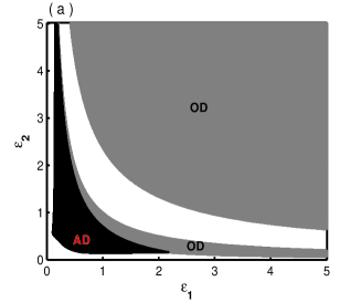
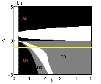
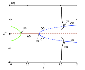
Figure 1: Coupled Van der Pol oscillators under cyclic coupling. HSS (AD) and IHSS (OD) islands in (a) ($\epsilon_{1}$-$\epsilon_{2}$) plane, (b) ($\Delta$ - $\epsilon$) plane. Black and gray regions represent AD and OD respectively. White region represents the coupled system is in oscillatory state. (c) Bifurcation diagram of cyclic coupling (taking parameters along the diagonal line of 1(a) or the yellow line of 1(b)) shows a transition from HSS to IHSS where extreme values of $x_{1}$ are plotted with coupling strength $\epsilon$. The coupled system undergoes transition from LC to AD at $\epsilon=0.3$ followed by a transition to OD at $\epsilon=0.86$. Further increase of $\epsilon$ another OD regime appears via a inverse Hopf Bifurcation(HB).

In this perspective, we use here a cyclic coupling scheme Dana_epjst in limit cycle systems as well as chaotic systems and try to understand the process of HSS-IHSS transition under a parameter mismatch. A cyclic coupling is generated by two separate interaction: a unidirectional diffusive coupling link which connects two oscillators in a forward direction via a pair of variables while another unidirectional link connects the oscillators in a reverse direction via a second pair of variables and thereby maintain a mutual interaction between the oscillations. The cyclic coupling thus defines a diffusion process or mutual exchange of information but do not involve the same pair of state variables of the oscillators. In the perspectives of engineering, under the cyclic coupling, one oscillator sends a signal via one pair of variables to the other oscillator while receives a feedback via another pair of variables Dana_epjst . In biological systems, this is similar to neuronal interactions where one neuron sends a signal via one pair of synaptic dendrites and receives a feedback via another pair Kandel . We first investigate two Van der Pol (VDP) oscillators under cyclic coupling. We find out a region of parameter mismatch where the HSS-IHSS transition occurs via the typical PB route.

Two coupled VDP oscillators under cyclic coupling are,

$$\dot{x}_{1}=\omega_{1}y_{1}+\epsilon_{1}(x_{2}-x_{1})$$

$$\dot{y}_{1}=b(1-x_{1}^{2})y_{1}-\omega_{1}x_{1}$$

$$\dot{x}_{2}=\omega_{2}y_{2}$$ (1)

$$\dot{y}_{2}=b(1-x_{2}^{2})y_{2}-\omega_{2}x_{2}+\epsilon_{2}(y_{1}-y_{2})$$

The first oscillator receives a signal from the second oscillator via the $x$-variable and sends a feedback via the $y$-variable which is expressed as cyclic coupling. $\epsilon_{1,2}$ is the coupling strength, $\omega_{1}$ and $\omega_{2}$ are the mismatch parameters and $b$=0.3. If we couple in reverse order i.e, the first oscillator is coupled with $\ y$ variable and second oscillator is coupled with $\ x$ variable the behavior of coupled systems and transition from HSS to IHSS are same. The coupled VDP system has a trivial fixed point $(0,0,0,0)$ which is the HSS solution of the system and the other fixed points (IHSS solutions) are $(x_{1}^{*},\>y_{1}^{*},\frac{\epsilon_{2}y_{1}^{*}}{\omega_{2}},0)$ where $y_{1}^{*}=\frac{\omega_{1}x_{1}^{*}}{b(1-x_{1}^{*2})}$ and $x_{1}^{*}=\pm\sqrt{1-\frac{\omega_{1}^{2}\omega_{2}+\epsilon_{1}\epsilon_{2}\omega_{1}}{b\omega_{2}\epsilon_{1}}}$.
Jacobian matrix at nonzero fixed point $(x_{1}^{*},y_{1}^{*},x_{2}^{*},y_{2}^{*})$ is given by

$$J=\left(\begin{array}[]{cccc}-\epsilon&\omega_{1}&\epsilon&0\\ p_{1}&p_{2}&0&0\\ 0&0&0&\omega_{2}\\ 0&\epsilon&p_{3}&p_{4}\par\end{array}\right)$$

where $p_{1}=-\omega_{1}-2bx_{1}^{*}y_{1}^{*},p_{2}=b(1-x_{1}^{*2}),p_{3}=-\omega_{2}-2bx_{2}^{*}y_{2}^{*}$ and $p_{4}=b(1-x_{2}^{*2})-\epsilon.$ The characteristic equation of the above Jacobian matrix is

$$\lambda^{4}+a_{1}\lambda^{3}+a_{2}\lambda^{2}+a_{3}\lambda+a_{4}=0$$ (2)

where $a_{1}=\epsilon-p_{2}-p_{4},\;\;a_{2}=-\epsilon p_{2}-\omega_{1}p_{1}-p_{3}\omega{2}-p_{4}\epsilon+p_{2}p_{4},\;\;a_{3}=p_{2}p_{4}\epsilon+\omega_{1}p_{1}p_{4}-p_{3}\omega_{2}\epsilon+p_{2}p_{3}\omega_{2},\;\;a_{4}=p_{2}p_{3}\omega_{2}\epsilon+p_{1}p_{3}\omega_{1}\omega_{2}-\epsilon^{2}p_{1}\omega_{2}.$

We check the stability of the equilibrium points as a function of $\epsilon_{1}$ and $\epsilon_{2}$ in Fig. 1(a) when $\omega_{1}=-\omega_{2}=1$. The trivial fixed point origin, i.e, the HSS(AD) is stable in the black region whereas the nontrivial fixed points, i.e, the IHSS are stable in the gray regions. The boundary between HSS(AD) and IHSS(OD) is given by the curve $\omega_{2}\epsilon_{1}b=\omega_{1}^{2}\omega_{2}+\epsilon_{1}\epsilon_{2}\omega_{1}$. The oscillatory states are represented by the narrow white regime of extreme left and in the extreme down. Interestingly, two sets of nontrivial fixed points exist, one group is stable in the upper gray region and the other set is stable in the lower gray region when we have taken, $\omega_{1}=1$ and $\omega_{2}=-1$ and the unstable island is shown between them as white regime. We explore the HSS and IHSS scenarios in a broader parameter space of $\Delta$- $\epsilon$ plane assuming $\epsilon_{1}=\epsilon_{2}=\epsilon$. Note that, for HSS and its transition to IHSS, a symmetry breaking parameter is necessary while the cyclic coupling is still maintaining a symmetry so far $\epsilon_{1}=\epsilon_{2}=\epsilon$. A parameter mismatch $\Delta=\frac{\omega_{2}}{\omega_{1}}$ introduces the essential asymmetry in the coupled system. We fix $\omega_{1}$ at +1 and vary $\omega_{2}$ continuously from -5 to +5 with a step size of 0.1 and draw the $\Delta$ vs $\epsilon$ plot in Fig. 1(b). For a positive mismatch, $\Delta>0$, the limit cycle (LC) eventually collapses to stable HSS. Further increase of coupling strength cannot induce IHSS in the coupled systems. On the other hand when $\Delta\sim 0$, a small HSS island exists since $\omega_{2}$ is too small and the uncoupled second oscillator which contains $\omega_{2}$ behaves like bursting. Obviously, for $\Delta\sim 1$, no death island appears due to a small or no mismatch of the coupled systems. However, distinct regions of LC, HSS and a direct transition from HSS to IHSS is clearly seen in the $\Delta<0$ region when $\omega_{2}$ has a negative value and it signifies a change of orientation of the trajectory or a counter-rotation Bhowmick ; Witkowski ; Prasad ; Newby of the Van der Pol system. Two oppositely rotating VDP oscillators show a HSS to IHSS transition when they are coupled via a type of cyclic coupling. Thus the negative parameter mismatch has a strong bearing on the HSS to IHSS transition as seen in the Fig. 1.

We derive the stability condition of the trivial fixed point origin assuming $\epsilon_{1}=\epsilon_{2}=\epsilon$ and $\Delta=-1$. The stability of the equilibrium origin is calculated from the Jacobian of the coupled VDP,

$$J=\left(\begin{array}[]{cccc}-\epsilon&\omega_{1}&\epsilon&0\\ -\omega_{1}&b&0&0\\ 0&0&0&\omega_{2}\\ 0&\epsilon&-\omega_{2}&b-\epsilon\par\end{array}\right)$$

with eigen values $\lambda=\frac{1}{2}[(b-\epsilon)\pm\sqrt{(b-\epsilon)^{2}+4k}]$ where $k=-\frac{1}{2}[-(1-b\epsilon)\pm\sqrt{4\epsilon^{2}+\epsilon^{2}b^{2}}]$. The stability condition of the fixed point origin is obtained as $b\leq\epsilon\leq\frac{1}{2}(-b+\sqrt{b^{2}+4})$. For a choice of $b=0.3$, HSS occurs in the coupling range $0.3\leq\epsilon\leq 0.86$ and the IHSS appears at $\epsilon=0.86$ which match with the numerical simulations along the horizontal line in Fig. 1 (b).

Further we have checked the nature of HSS to IHSS transition using the MATCONT tool Dhooge and plotted the extrema of $x_{1}$ with coupling strength $\epsilon$ in Fig.1(c) for $b=0.3$ and $\omega_{1}=-\omega_{2}=1$. For a coupling strength $\epsilon<0.3$ the coupled system shows limit cycle behavior. At $\epsilon=0.3$, the coupled system stabilizes to the HSS via Hopf bifurcation (HB) and it continues until $\epsilon=0.86$ when two stable nonzero equilibrium points i.e. IHSS appear via PB and continues up to 1. It is to be noted that if $\omega_{1}=-\omega_{2}=1$ and $\epsilon=1$, $x_{1}^{*}$ becomes 1 and $y_{1}^{*}$ becomes undefined which creates a singularity at $\epsilon=1$. With further increase of $\epsilon$ ($\epsilon>1$) an unstable limit cycle appears which eventually goes to a stable limit cycle (The extrema is shown by black line) with high amplitude at $\epsilon=~{}1.6$. Further increase of $\epsilon$ generates another IHSS becomes stable via inverse HB and is shown by solid blue line in Fig.1(c). The MATCONT plot basically confirmed the analytical prediction whereas the nature of transition matches with Fig 1(a) along diagonal line or the yellow line of the Fig1(b).

An immediate question arises how the coupled VDP oscillator would behave if the negative mismatch ($\Delta=-1$) is introduced under the typical diffusive coupling instead of the cyclic coupling? For this we consider two diffusively coupled VDP systems,

$$\dot{x}_{1}=\omega_{1}y_{1}+\epsilon_{1}(x_{2}-x_{1})$$

$$\dot{y}_{1}=b(1-x_{1}^{2})y_{1}-\omega_{1}x_{1}+\epsilon_{2}(y_{2}-y_{1})$$

$$\dot{x}_{2}=\omega_{2}y_{2}+\epsilon_{1}(x_{1}-x_{2})$$

$$\dot{y}_{2}=b(1-x_{2}^{2})y_{2}-\omega_{2}x_{2}+\epsilon_{2}(y_{1}-y_{2})$$ (3)

Consider two types of diffusive coupling through one variable i.e, (i) $\epsilon_{1}=0,\epsilon_{2}\neq 0$ or (ii) $\epsilon_{1}\neq 0,\epsilon_{2}=0$. In the first type of coupling $x_{1}-x_{2}$ will be in anti-synchronization state and $y_{1}-y_{2}$ are in complete synchronization state i.e, mixed synchronization is occurred Bhowmick ; Bhowmick2 for $\omega_{2}=-\omega_{1}$. Again $x_{1}-x_{2}$ are in complete synchronization and $y_{1}-y_{2}$ are in anti synchronization state for the second type of coupling. Other possible choice of couplings are explained in details in Ref Bhowmick ; Bhowmick2 . Death scenario i.e HSS or IHSS state is only possible when $\epsilon_{1}\neq 0,\epsilon_{2}\neq 0$. In our study, for simplicity, we consider $\epsilon_{1}=\epsilon_{2}=\epsilon$. One of the solution of system (3) is (0, 0, 0, 0). The characteristic equation of coupled system (3) at origin is given by equation (2), where $a_{1}=4\epsilon-2b,\;\;a_{2}=4\epsilon^{2}+b^{2}-6\epsilon b+2,\;\;a_{3}=4\epsilon-2b-4\epsilon^{2}b+2b^{2}\epsilon$ and $a_{4}=1-2b\epsilon.$ Using Routh-Hurwitz criteria the origin i.e. HSS state is stable for $0.15\leq\epsilon\leq 1.66.$

Numerical study of HSS-IHSS transition of coupled Van der Pol oscillators is shown in Fig. 2 where the bifurcation diagram shows a HSS window (solid blue line) in a range of coupling strength and appears via HB. At the left side of the HSS window, a stable LC (solid gray line) exists where the trivial fixed point origin is unstable (dashed blue line). A transition from HSS to IHSS occurs at the right side of the HSS window via PB at $\epsilon=1.66$. Beyond the PB point, two distinctly new stable equilibrium points (solid brown line) are created as IHSS lines and coexist with the unstable fixed point origin (dashed blue line).

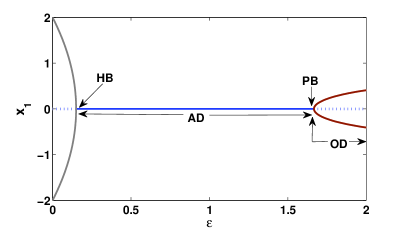
Figure 2: Bidirectionally coupled Van der Pol oscillators. MATCONT plot shows a transition from HSS to IHSS. HSS appears via HB from oscillatory state at $\epsilon=0.15$ whereas IHSS occur via PB at $\epsilon=1.66$.

Thus, in another limit cycle system such as the VDP oscillator, the HSS-IHSS transition occurs via PB as usual irrespective of the type of coupling, typical diffusive or cyclic and the nature of parameter mismatch. Next we focus on chaotic oscillators using similar coupling strategies (cyclic and diffusive) and a negative parameter mismatch in search of other bifurcation route if at all exists besides the TB and the SNB under repulsive coupling Hens .

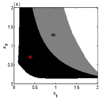
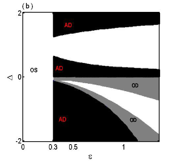
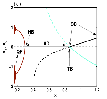
Figure 3: Coupled chaotic Sprott systems under cyclic coupling. The HSS and IHSS islands in (a) $\epsilon_{1}$-$\epsilon_{2}$ and (b) $\epsilon-\Delta$ plane. Black color represents the HSS (AD) region and grey lines are the boundaries of IHSS (OD) region. (c) Extremum of $x_{1}$ and $x_{2}$ is plotted with varying $\epsilon$ which corresponds to parameters along the diagonal line $\epsilon_{1}=\epsilon_{2}$ in (a) and $\Delta=-1$ line in (b). A transition from LC to AD is seen at $\epsilon=0.3$ followed by a transition to OD at $\epsilon=0.86$.

For numerical study, we consider two chaotic Sprott oscillators under cyclic coupling appear as,

$$\dot{x}_{1}=x_{1}y_{1}-\omega_{1}z_{1}+\epsilon_{1}(x_{2}-x_{1})$$

$$\dot{y}_{1}=x_{1}-y_{1}$$

$$\dot{z}_{1}=\omega_{1}x_{1}+az_{1}$$

$$\dot{x}_{2}=x_{2}y_{2}-\omega_{2}z_{2}$$

$$\dot{y}_{2}=x_{2}-y_{2}$$

$$\dot{z}_{2}=\omega_{2}x_{2}+az_{2}+\epsilon_{2}(z_{1}-z_{2})$$ (4)

The Sprott oscillator is chaotic in isolation for $a=0.3$; one oscillator sends a signal via $x$ variable and receives a feedback via $z$ variable which is expressed as cyclic coupling. The fixed points are given by the origin $(0,0,0,0,0,0)$ and the $(x_{1}^{*},y_{1}^{*},z_{1}^{*},x_{2}^{*},y_{2}^{*},z_{2}^{*})$ where $y_{1}^{*}=x_{1}^{*},z_{1}^{*}=-\frac{\omega_{1}x_{1}^{*}}{a},x_{2}^{*}=\frac{1}{\epsilon_{1}}(\epsilon_{1}x_{1}^{*}-\frac{\omega_{1}^{2}x_{1}^{*}}{a}-x_{1}^{*2}),y_{2}^{*}=x_{2}^{*},z_{2}^{*}=\frac{x_{2}^{*2}}{\omega_{2}}$ where $x_{1}^{*}$ is the real root of the cubic equation given by $\frac{\omega_{2}}{\epsilon_{1}}(\epsilon_{1}-\frac{\omega_{1}^{2}}{a}-x_{1}^{*})+\frac{(a-\epsilon_{2})x_{1}^{*}}{\omega_{2}\epsilon_{1}^{2}}(\epsilon_{1}-\frac{\omega_{1}^{2}}{a}-x_{1}^{*})^{2}-\frac{\omega_{1}\epsilon_{2}}{a}=0$.

We induce a negative parameter mismatch $\Delta=\frac{\omega_{2}}{\omega_{1}}=-1$ as an asymmetry in the coupled system when the two oscillators are in counter-motion Bhowmick ; Witkowski ; Prasad ; Newby . Assuming $\epsilon_{1}=\epsilon_{2}=\epsilon$, the cubic equation in $x_{1}^{*}$ is found to have a singularity at $\epsilon=a=0.3$. For $\epsilon<0.3$ the equation has three non-zero real roots which are unstable and just after $\epsilon>0.3$ the equation has only one non-zero real root. This non-zero real root is unstable for $0.3<\epsilon<0.86$ whereas the HSS is stable. The eigenvalues of the Jacobian matrix of system (4) at origin are $\lambda_{1}=-1.0,\lambda_{2}=-1.0$ and other eigenvalues are the roots of the equation given by (2) where $a_{1}=2(\epsilon-a),\;\;a_{2}=\omega_{1}^{2}+\omega_{2}^{2}-3a\epsilon+\epsilon^{2}+a^{2},\;\;a_{3}=(\epsilon-a)(\omega_{1}^{2}+\omega_{2}^{2}-a\epsilon),$ and $a_{4}=\omega_{1}^{2}\omega_{2}^{2}+\epsilon^{2}\omega_{1}\omega_{2}-a\epsilon\omega_{2}^{2}.$ Using Routh-Hurwitz criteria, HSS is found to be stable in the range $0.3<\epsilon<0.86.$

At $\epsilon\geq 0.86$, IHSS appears and HSS become unstable via transcritical bifurcation (TB). Further we expand the regime of HSS and its transition to IHSS by drawing $\epsilon_{1}-\epsilon_{2}$ and $\epsilon-\Delta$ phase space diagram in Fig. 3(a) and 3(b) respectively. For both the figures, HSS is shown in black color whereas IHSS is depicted in grey color. The transition from HSS to IHSS is only possible when $\Delta<0$. Extreme values of $x_{1}$ and $x_{2}$ are plotted with $\epsilon$ as illustrated in Fig. 3(c) using the software package MATCONT Dhooge for $\Delta=-1.0$. The chaotic dynamics becomes period-1 for weak coupling via quasiperiodic (QP) route and then the origin becomes stable as a HSS state via HB. Finally, the equilibrium origin loses its stability (from solid gray line to grey dotted line) and the unstable non-zero equilibrium points become stable as indicated by solid black lines and solid green lines. The HSS transits to IHSS via a TB at a larger coupling strength. A similar HSS-IHSS transition has also been observed in coupled chaotic oscillators under repulsive interaction Hens ; Hens2 . Note that, the white regimes in the right side of Fig. 3(a) and between two OD islands in Fig. 3(b) are unstable. We have checked that OD island ends via HB and goes to the unstable regime. We focus here only at the emergence of HSS and its transition to IHSS.

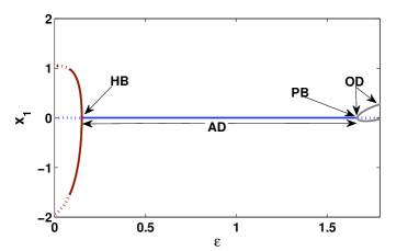
Figure 4: Coupled chaotic Sprott systems under diffusive coupling. Bifurcation diagram shows a transition of HSS (AD) to IHSS (OD) with varying coupling strength $\epsilon$. Extrema of $x_{1}$ has been plotted against $\epsilon$. Solid brown line represents Limit cycle oscillator where dotted blue line represents unstable region of LC. Solid blue line signifies HSS which occurs via HB and solid grey line in the right side represent two stable branch appears through PB which coexists with unstable origin.

Finally, we search the transition scenario in coupled Sprott oscillators under the conventional diffusive bidirectional coupling. Two coupled Sprott systems under diffusive bidirectional coupling are given by

$$\dot{x}_{1}=x_{1}y_{1}-\omega_{1}z_{1}+\epsilon_{1}(x_{2}-x_{1})$$

$$\dot{y}_{1}=x_{1}-y_{1}$$

$$\dot{z}_{1}=\omega_{1}x_{1}+az_{1}+\epsilon_{2}(z_{2}-z_{1})$$

$$\dot{x}_{2}=x_{2}y_{2}-\omega_{2}z_{2}+\epsilon_{1}(x_{1}-x_{2})$$

$$\dot{y}_{2}=x_{2}-y_{2}$$

$$\dot{z}_{2}=\omega_{2}x_{2}+az_{2}+\epsilon_{2}(z_{1}-z_{2})$$ (5)

Clearly, the coupled system has a equilibrium point at origin. For simplicity, the coupling strengths are taken identical $\epsilon_{1}=\epsilon_{2}=\epsilon$. We draw a bifurcation diagram with varying the coupling strength $\epsilon$ in Fig. 4 using the MATCONT software.

Figure 4 shows a transition from the HSS to the IHSS. For lower coupling, an unstable equilibrium origin (dashed line) coexists with stable LC (solid brown line). Increasing the coupling strength HSS (solid blue line) originates via a HB. A further increase of coupling strength induces a transition to two separate branches of IHSS states via PB as usually found for all other forms of diffusive coupling Volkov ; Kurths-pre ; Banerjee .

In summary, we numerically and analytically investigate a transition from HSS to IHSS for coupled limit cycle and also for coupled chaotic oscillators when their parameters are detuned. We use a VDP oscillator as paradigmatic model for limit cycle and sprott oscillator as chaotic model. To investigate the transition phenomena, we introduce cyclic coupling as well as conventional diffusive coupling when the oscillators have negative parameter mismatch. We notice, conjugate effect of cyclic/diffusive coupling with detuned negative mismatch breaks the symmetry of the coupled system. In the limit cycle oscillators such as the VDP model under symmetric cyclic coupling or diffusive coupling, the HSS to IHSS transition appears via PB, as usually true for other limit cycle systems, so far investigated, irrespective of the coupling forms. On the other hand, for a chaotic Sprott system under cyclic coupling, the transition occurred via TB as reported earlier for other chaotic systems under a combination of diffusive and repulsive mean field interaction. However, we find that the transition from HSS to IHSS in chaotic Sprott system follows a PB when two of them are coupled with the conventional diffusive bidirectional coupling. A transition of a homogeneous medium to stable patterns was first noticed by Turing Turing . Very recently this becomes sudden issue of interest when a similar transition from a stable HSS to multiple IHSS state was reported Volkov in Landau-Stuart (LS) limit cycle system. While most of the studies focused on the LS system only using different coupling forms Volkov ; Kurths-pre ; Banerjee1 , none of them gives attention to chaotic system if such a transition could appear except by using a repulsive mean-field interaction Hens ; Hens2 . Under cyclic or diffusive coupling in different negatively detuned mismatch oscillators we examine the phenomenon of HSS to IHSS with strong numerical and analytical evidence.

Acknowledgments: Authors would like to thank an anonymous referee for constructive criticisms and suggestions which has helped in improving the manuscript in its present form. They also thank S. K. Dana for useful discussions.

References

- (1) G. Saxena, A. Prasad, R Ramaswamy, Amplitude death: the emergence of stationarity in coupled nonlinear systems, Phys. Rep 521(5) (2012) 205-28.
- (2) A. Koseska, E. Volkov, J. Kurths, Oscillation quenching mechanisms: Amplitude vs. Oscillation death, Phys. Rep 531 (2013) 173-99.
- (3) E. Ullner, A. Zaikin, E.I. Volkov, J.G. Ojalvo, Multistability and Clustering in a Population of Synthetic Genetic Oscillators via Phase-Repulsive Cell-to-Cell Communication, Phys. Rev. Lett. 99 (2007) 148103-6. A. Koseska, E.I. Volkov, A. Zaikin, J. Kurths, Inherent multi stability in arrays of autoinducer coupled genetic oscillators, Phys. Rev. E 75 (2007) 031916-23.
- (4) J.J. Suárez-Vargas, J.A. González, A. Stefanovska, P.V.E. McClintock, Diverse routes to oscillation death in a coupled-oscillator system. Euro. Phys. Letts. 85(3) (2009) 38008.
- (5) M. Yoshimoto, K. Yoshikawa, Y. Mori, Coupling among three chemical oscillators: Synchronization, phase death, and frustration, Phys. Rev. E 47 (1993) 864-74.
- (6) K. Bar-Eli, On the stability of coupled chemical oscillators, Physica D ( Amsterdam) 14 (1985) 242-52.
- (7) D.G. Aronson, G.B. Ermentrout, N. Kopell, Amplitude response of coupled oscillators, Physica D 41 (1990) 403-49. P.C. Matthews, R.E. Mirollo, S.H. Strogatz, Dynamics of a large system of coupled nonlinear oscillators, Physica D 52 (1991) 293-331.
- (8) D.V. Ramana Reddy, A. Sen, G.L. Johnston, Time Delay Induced Death in Coupled Limit Cycle Oscillators, Phys. Rev. Lett. 80 (1998) 5109-12.
- (9) K. Konishi, Amplitude death induced by dynamic coupling, Phys. Rev. E 68 (2003) 067202.
- (10) V. Resmi, G. Ambika, R.E. Amritkar, General mechanism for amplitude death in coupled systems, Phys. Rev. E 84 (2011) 046212.
- (11) R. Karnatak, R. Ramaswamy, A. Prasad, Amplitude death in the absence of time delays in identical coupled oscillators, Phys. Rev. E 76 (2007) 035201.
- (12) C.R. Hens, O.I. Olusola, P. Pal, S.K. Dana. Oscillation death in diffusively coupled oscillators by local repulsive link, Phys. Rev. E 88 (2013) 034902.
- (13) A.Koseska, E. Volkov, J. Kurths, Transition from Amplitude to Oscillation Death via Turing Bifurcation, Phys. Rev. Lett. 111 (2013) 024103.
- (14) W. Zou, D.V. Senthilkumar, A. Koseska, J. Kurths, Generalizing the transition from amplitude to oscillation death in coupled oscillators, Phys. Rev. E 88 (2013) 050901.
- (15) T. Banerjee, D. Biswas, Amplitude death and synchronized states in nonlinear time-delay systems coupled through mean-field diffusion, Chaos 23 (2013) 043101.
- (16) T. Banerjee, D. Ghosh, Transition from amplitude to oscillation death under mean-field diffusive coupling, Phys. Rev. E 89 (2014) 052912. T, Banerjee, D. Ghosh, Experimental observation of a transition from amplitude to oscillation death in coupled oscillators, Phys. Rev. E 89 (2014) 062902.
- (17) C.R. Hens, P. Pal, S.K. Bhowmick, P.K. Roy, A. Sen, S.K. Dana, Diverse routes of transition from amplitude to oscillation death in coupled oscillators under additional repulsive links, Phys. Rev. E 89 (2014) 032901. M. Nandan, C.R Hens, P. Pal, S.K. Dana, Transition from amplitude to oscillation death in a network of oscillators, Chaos 24 (2014) 043103.
- (18) B. Ermentrout, N. Kopell, Oscillator death in systems of coupled neural oscilltors, SIAM J. Appl. Math. 50 (1990) 125-46.
- (19) N. Suzuki, C. Furusawa, K. Kaneko, Oscillatory Protein Expression Dynamics Endows Stem Cells with Robust Differentiation Potential, PLoS One 6 (2011) e27232.
- (20) A. Koseska, E. Ullner, E.I. Volkov, J. Kurths, J.G. Ojalvo, Cooperative differentiation through clustering in multicellular opulations, J. Theor. Biol. 263 (2010) 189-202.
- (21) D. Ruwisch, M. Bode, D. Volkov, E.I. Volkov, Collective modes of three coupled relaxation oscillators: the influence of detuning, Int. J. Bifurcation Chaos 9 (1999) 1969-1981.
- (22) A. Turing, The Chemical Basis of Morphogenesis, Phil. Trans. R. Soc. B 237 (1952) 37-72.
- (23) M.K.T. Kamal, P.R. Sharma, M.D. Shrimali’ Suppression of oscillations in mean-field diffusion. Pramana, in press(2014).
- (24) P.R. Sharma, A. Sharma, M.D. Shrimali, A. Prasad, Targeting fixed-point solutions in nonlinear oscillators through linear augmentation, Phys. Rev. E 83 (2011) 067201.
- (25) O.I. Olusola, A.N. Njah, S.K. Dana, Synchronization in chaotic oscillators by cyclic coupling, Eur Phys. J. Special Topics 222 (2013) 927-37.
- (26) E. Kandel, J. Schwartz, T. Jessell, Principles of neural science McGraw-Hill USA 2000.
- (27) S.K. Bhowmick, D. Ghosh, S.K. Dana, Synchronization in counter-rotating oscillators, Chaos 21 (2011) 033118.
- (28) B. Witkowski, P. Perlikowski, A. Prasad, T. Kapitaniak, The dynamics of co- and counter rotating coupled spherical pendula, Eur Phys. J. Special Topics 223(4) (2014) 707-20.
- (29) A. Prasad, Universal occurrence of mixed-synchronization in counter-rotating nonlinear coupled oscillators, Chaos Soliton Fractals 43 (2010) 42-6.
- (30) J.M. Newby, M.A. Schwemmer, Effects of Moderate Noise on a Limit Cycle Oscillator: Counterrotation and Bistability, Phys. Rev. Lett. 112 (2014) 114101.
- (31) A. Dhooge, W. Govaerts, Y.A. Kuznetsov, MATCONT, ACM Trans. Math. Softw. 29 (2003) 141.
- (32) S.K. Bhowmick, B.K. Bera, D. Ghosh, Generalized counter-rotating oscillators: mixed synchronization, Commun Nonlinear Sci Numer Simulat, 22 (2015) 692-701.