A symmetry breaking transition in the edge/triangle network model

Abstract

Our general subject is the emergence of phases, and phase transitions, in large networks subjected to a few variable constraints. Our main result is the analysis, in the model using edge and triangle subdensities for constraints, of a sharp transition between two phases with different symmetries, analogous to the transition between a fluid and a crystalline solid.

Key words. Graph limits, entropy, bipodal structure, phase transitions, symmetry breaking

1 Introduction

Our general subject is the emergence of phases, and phase transitions, in large networks subjected to a few variable constraints, which we take as the densities of a few chosen subgraphs. We follow the line of research begun in [17] in which, for $k$ given constraints on a large network one determines a global state on the network, by a variational principle, from which one can compute a wide range of global observables of the network, in particular the densities of all subgraphs. A phase is then a region of constraint values in which all these global observables vary smoothly with the constraint values, while transitions occur when the global state changes abruptly. (See [5, 6, 17, 18, 16, 7] and the survey [15].) Our main focus is on the transition between two particular phases, in the system with the two constraints of edge and triangle density: phases in which the global states have different symmetry.

If one describes networks (graphs) on $n$ nodes by their $n\times n$ adjacency matrices, we will be concerned with asymptotics as $n\to\infty$, and in particular limits of these matrices considered as $0$-$1$ valued graphons. (Much of the relevant asymptotics is a recent development [1, 2, 8, 9, 10]; see [11] for an encyclopedic treatment.) Given $k$ subgraph densities as constraints, the asymptotic analysis in [17] leads to the study of one or more $k$-dimensional manifolds embedded in the infinite dimensional metric space $W$ of (reduced) graphons, the points in the manifold being the emergent (global) states of a phase of the network. That is, there are smooth embeddings, of open connected subsets (called phases) of the phase space $\Gamma\subset[0,1]^{k}$ of possible constraint values, into $W$. The embeddings are obtained from the constrained entropy density $s(P)$, a real valued function of the constraints $P\in\Gamma$, through the variational principle [17, 18]: $s(P)=\sup\{{\cal S}(g)\,|\,C(g)=P\}$, the constraints being described by $C(g)=P$, for instance edge density $\varepsilon(g)=P_{1}$ and triangle density $\tau(g)=P_{2}$, and ${\cal S}$ being the negative of the large deviation rate function of Chatterjee-Varadhan [4].

The above framework is modeled on that of statistical physics in which the system is the simultaneous states of many interacting particles, the constraints are the invariants of motion (mass and energy densities for simple materials) and the global states, ‘Gibbs states’, can be understood in terms of conditional probabilities [22]. The relevant variational principle was proven in [21]. In contrast, for large graphs the constrained entropy optima turn out to be much easier to analyze than Gibbs states. First, it has been found that in all known cases entropy optima are ‘multipodal’, i.e. for each phase in any graph model they lie in some $M$ dimensional manifold in $W$ corresponding to a decomposition of all the nodes into $M$ equivalence classes [5, 6, 7]. This brings the embedding down into a fixed finite dimension, at least within each phase, in place of the infinite dimensions of $W$. In practice, for $k=2$ this often allows one to find an embedding into 4 dimensions, so it only remains to understand how our 2 dimensional surface sits in those 4 dimensions. The main goal of this paper is to study this near a particular transition for edge/triangle constraints.

Figure 1: Left: Boundary of the phase space for subgraph constraints edges and triangles. The scalloped region is exaggerated for better visualization; Right: Boundaries of phases I, II and III.

The phase space $\Gamma$ of possible values of edge/triangle constraints is the interior of the scalloped triangle of Razborov [19], sketched in Figure 1. Extensive simulation in this model [16] shows the existence of several phases, labeled $I$, $II$ and $III$ in Figure  1.

Figure 2: Erdos-Renyi curve and phases I, II and III

The main focus of this paper is the transition between phases $II$ and $III$. There is good simulation evidence, but there is still no proof of this transition. What we will do is assume, as seen in simulation, that all entropy optimal graphons for edge/triangle densities near the transition are bipodal, that is given by a piecewise constant function of the form:

$$g(x,y)=\begin{cases}a&x,y<c,\cr d&x<c<y,\cr d&y<c<x,\cr b&x,y>c.\end{cases}$$ (1)

Bipodal graphons are generalizations of bipartite graphons, in which $a=b=0$. Here $c,a,d$ and $b$ are constants taking values between 0 and 1. We do not assume these entropy optimizers are unique. But from the bipodal assumption we can prove uniqueness, and also derive, as shown already in [16], the equations determining the transition curve, and prove that the optimal graphons for edge/triangle constraints $(\varepsilon,\tau)$ to the left of the transition, have the form:

$$g(x,y)=\begin{cases}\varepsilon-(\varepsilon^{3}-\tau)^{1/3}&x,y<1/2\hbox{ or }x,y>1/2\cr\varepsilon+(\varepsilon^{3}-\tau)^{1/3}&x<\frac{1}{2}<y\hbox{ or }y<\frac{1}{2}<x,\end{cases}$$ (2)

which is highly symmetric in the sense that $c=1/2$ and $a=b$. The main result of this paper is the derivation of the lower order terms in $\varepsilon$ and $\tau$ of the bipodal parameters $a,b,c,d$ as the constraints move to the right of the transition, i.e. we determine how the symmetry is broken at the transition. Before we get into details we should explain the connection between this study of emergent phases and their transitions, and other work on random graphs using similar terminology.

The word phase is used in many ways in the literature, but ‘emergent phase’ is more specific and refers to a coherent, large scale description of a system of many similar components, in the following sense. Consider large graphs, thought of as systems of many edges on a fixed number of labeled nodes. To work at a large scale means to be primarily concerned with global features or observables, for instance densities of subgraphs.

Finite graphs are fully described (i.e. on a small scale) by their adjacency matrices. In the graphon formalism these have a scale-free description in which each original node is replaceable by a cluster of $m$ nodes, which makes for a convenient analysis connecting large and small scale.

Phases are concerned with large graphs under a small number $k$ of variable global constraints, for instance constrained by the 2 subdensities of edges and triangles. We say one or more phases emerge for such systems, corresponding to one or more open connected subsets of parameter values, if: 1) there are unique global states (graphons) associated with the sets of constraint values; 2) the correspondence defines a smooth $k$-dimensional surface in the infinite dimensional space of states.

Note that not all achievable parameter values (the phase space) belong to phases, in particular the boundary of the phase space does not. In fact emergent phases are interesting in large part because they exhibit interesting (singular) boundary behavior in the interior of the phase space. For graphs we see this in at least two ways familiar from statistical mechanics. In the edge/2-star model there is only one phase but there are achievable parameter values with multiple states associated (as in the liquid/gas transition); see Figure 3.

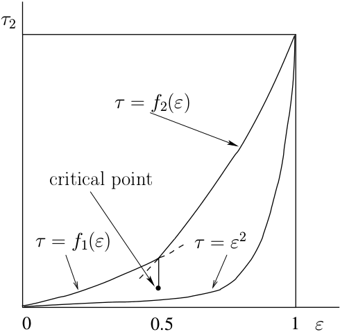
Figure 3: Transition ending in a critical point for edge/2-star model

In most models constraint values on the Erdös-Rényi curve – parameter values corresponding to iid edges – provide unique states which however do not vary smoothly across the curve, and this provides boundaries of phases [17]. For edge/triangle constraints there is another phase boundary associated with a loss of symmetry (as in the transition between fluid and crystalline solid). In all models studied so far phases make up all but a lower dimensional subset of the phase space but this may not be true in general.

From an alternative vantage random graphs are commonly used to model some particular network, the idea being to fit parameter values in a parametric family of probability distributions on some space of possible networks, so as to get a manageable probabilistic picture of the one target network of interest; see [3, 12] and references therein. The one parameter Erdös-Rényi (ER) family is often used this way for percolation, as are multiparameter generalizations such as stochastic block models and exponential random graph models (ERGMs). Asymptotics is only a small part of such research, and for ERGMs it poses some difficulties as is well described in [3]

Newman et al considered phase transitions for ERGMs; see [13] for a particularly relevant example. Chatterjee-Varadhan introduced in [4] a powerful asymptotic formalism for random graphs with their large deviations theorem, within the previously developed graphon formalism. This was applied to ERMGs in [3], which was then married with Newman’s phase analysis in [20] and numerous following works.

We now contrast this use of the term phase with the emergent phase analysis discussed above. In the latter a phase corresponds to an embedding of part of the parameter space into the emergent (global) states of the network, so transitions could be interpreted as singular behavior as those global network states varied. For ERGMs it was shown in [3] that the analogous map from the parameter space $\Gamma$ into $W$, determined by optimization of a free energy rather than entropy, is often many-to-one; for instance all states of the 2-parameter edge/2-star ERGM model actually belong to the 1-parameter ER family. Therefore transitions in an ERGM are naturally understood as asymptotic behavior of the model under variation of model parameters, rather than singular behavior among naturally varying global states of a network; in keeping with its natural use, a transition in an ERGM says more about the model than about constrained networks.

2 Outline of the calculation

The purpose of this calculation is to understand the transition, in the edge/triangle model, between phases $II$ and $III$ in Figure 1. We take as an assumption that our optimizing graphon at fixed constraint $(\varepsilon,\tau)$ is bipodal as in (1), and with $c$ being the size of the first cluster of nodes. We denote this graphon by $g_{abcd}$; see Figure 4. With the notation

$$S_{o}(z)=-\frac{1}{2}[z\ln(z)+(1-z)\ln(1-z)],\ 0\leq z\leq 1$$ (3)

and

$${\cal S}(g)=\int_{[0,1]^{2}}S_{o}[g(x,y)]\,dxdy,$$ (4)

to obtain $s(P)$ we maximize ${\cal S}(g_{abcd})$ by varying the four parameters $(a,b,c,d)$ while holding $P=(\varepsilon,\tau)$ fixed.

It is not hard to check that the symmetric graphon with $a=b=\varepsilon+(\tau-\varepsilon^{3})^{1/3}$, $c=\frac{1}{2}$ and $d=\varepsilon-(\tau-\varepsilon^{3})^{1/3}$ is always a stationary point of the functional ${\cal S}$. But is it a maximum? Near the choices of $(\varepsilon,\tau)$ where it ceases to be a maximum, what does the actual maximizing graphon look like?

We answer this by doing our constrained optimization in stages. First we fix $c$ and vary $(a,b,d)$ to maximize ${\cal S}(g)$ subject to the constraints on $\varepsilon$ and $\tau$. Call this maximum value $S(c)$. Since the graphon with parameters $(b,a,1-c,d)$ is equivalent to $(a,b,c,d)$, $S(c)$ is an even function of $c-\frac{1}{2}$. We expand this function in a Taylor series:

$$S(c)=S(\frac{1}{2})+\frac{1}{2}\ddot{S}(\frac{1}{2})(c-\frac{1}{2})^{2}+\frac{1}{24}\ddddot{S}(\frac{1}{2})(c-\frac{1}{2})^{4}+\cdots$$ (5)

where dots denote derivatives with respect to $c$.

If $\ddot{S}(\frac{1}{2})$ is negative, then the symmetric graphon is stable against small changes in $c$. If $\ddot{S}(\frac{1}{2})$ becomes positive (as we vary $\varepsilon$ and $\tau$), then the local maximum of $S(c)$ at $c=\frac{1}{2}$ becomes a local minimum. As long as $\ddddot{S}(\frac{1}{2})<0$, new local maxima will appear at $c\approx\frac{1}{2}\pm\sqrt{-6\ddot{S}(\frac{1}{2})/\ddddot{S}(\frac{1}{2})}$. In this case, as we pass through the phase transition, we should expect the optimal $|c-\frac{1}{2}|$ to be exactly zero on one side of the transition line (i.e., in the symmetric phase), and to vary as the square root of the distance to the transition line on the other (asymmetric) side.

If $\ddddot{S}(\frac{1}{2})$ is positive when $\ddot{S}(\frac{1}{2})$ passes through zero, something very different happens. Although $c=\frac{1}{2}$ is a local maximum whenever $\ddot{S}(\frac{1}{2})<0$, there are local maxima elsewhere, at locations determined largely by the higher order terms in the Taylor expansion (5). When $\ddot{S}(\frac{1}{2})$ passes below a certain threshold, one of these local maxima will have a higher entropy than the local maximum at $c=\frac{1}{2}$, and the optimal value of $c$ will change discontinuously.

The calculations below give analytic formulas for $\ddot{S}(\frac{1}{2})$ and $\ddddot{S}(\frac{1}{2})$ as functions of $\varepsilon$ and $\tau$. We can then evaluate these formulas numerically to fix the location of the phase transition curve and determine which of the previous two paragraphs more accurately describes the phase transition near a given point on that curve. We then compare these results to numerical sampling that is done without the simplifying assumption that optimizing graphons are bipodal.

Our results indicate that

• The assumption of bipodality is justified, and

• $\ddddot{S}(\frac{1}{2})$ remains negative on the phase transition curve, implying that $c$ does not change discontinuously. Rather, $|c-\frac{1}{2}|$ goes as the square root of the distance to phase transition curve, in the asymmetric bipodal phase.

3 Exact formulas for $\ddot{S}(\frac{1}{2})$ and $\ddddot{S}(\frac{1}{2})$

We now present the details of our perturbation calculations in detail.

3.1 Varying $(a,b,d)$ for fixed $c$.

The first step in the calculation is to derive the variational equations for maximizing ${\cal S}(g_{abcd})$ for fixed $(\varepsilon,\tau,c)$. We first express the edge and triangle densities and $S={\cal S}(g_{abcd})$ as functions of $(a,b,c,d)$:

Figure 4: The parameter set $(a,b,c,d)$ of a bipodal graphon.

$$\varepsilon = c^{2}a+2c(1-c)d+(1-c)^{2}b$$ (6)

$$\tau = c^{3}a^{3}+3c^{2}(1-c)ad^{2}+3c(1-c)^{2}bd^{2}+(1-c)^{3}b^{3}$$ (7)

$$S = c^{2}S_{o}(a)+(1-c)^{2}S_{o}(b)+2c(1-c)S_{o}(d)$$ (8)

Next we compute the gradient of these quantities with respect to $(a,b,d)$, where $\nabla_{3}$ is an abbreviation for $(\partial_{a},\partial_{b},\partial_{d})$:

$$\nabla_{3}\,\varepsilon= (c^{2},(1-c)^{2},2c(1-c))$$ (9)

$$\nabla_{3}\,\tau= (3c^{3}a^{2}+3c^{2}(1-c)d^{2},3(1-c)^{3}b^{2}+3c(1-c)^{2}d^{2},$$ (11)

$$\qquad\qquad\qquad 6c^{2}(1-c)ad+6c(1-c)^{2}bd)$$

$$\nabla_{3}\,S= (c^{2}S_{o}^{{}^{\prime}}(a),(1-c)^{2}S_{o}^{{}^{\prime}}(b),2c(1-c)S_{o}^{{}^{\prime}}(d))$$ (12)

At a maximum of $S$ (for fixed $c$, $\varepsilon$ and $\tau$), $\nabla_{3}\,S$ must be a linear combination of $\nabla_{3}\,\varepsilon$ and $\nabla_{3}\,\tau$ so

$$0= \det\begin{pmatrix}\nabla_{3}\,\varepsilon\cr\nabla_{3}\,\tau\cr\nabla_{3}\,S\cr\end{pmatrix}$$ (13)

$$= c^{2}(1-c)^{2}6c(1-c)$$ (15)

$$\times\det\begin{pmatrix}1&1&1\cr a^{2}c+d^{2}(1-c)&d^{2}c+b^{2}(1-c)&cad+(1-c)bd\cr S_{o}^{{}^{\prime}}(a)&S_{o}^{{}^{\prime}}(b)&S_{o}^{{}^{\prime}}(d)\cr\end{pmatrix}$$

Expanding the determinant and dividing by $6c^{3}(1-c)^{3}$, we obtain

$$0=f(a,b,c,d) := \phantom{+}S_{o}^{{}^{\prime}}(a)[cd(a-d)-(1-c)b(b-d)]$$ (18)

$$+S_{o}^{{}^{\prime}}(b)[ca(a-d)-(1-c)d(b-d)]$$

$$+S_{o}^{{}^{\prime}}(d)[c(d^{2}-a^{2})+(1-c)(b^{2}-d^{2})].$$

3.2 Strategy for varying $c$

We just showed how optimizing the entropy for fixed $\varepsilon$, $\tau$, and $c$ is equivalent to setting $f=0$. From now on we treat $f=0$ as an additional constraint. The three constraint equations $\varepsilon=\varepsilon_{o}$, $\tau=\tau_{o}$, $f=0$ define a curve in $(a,b,d,c)$ space, which we can parametrize by $c$. Since $\varepsilon$, $\tau$ and $f$ are constant, derivatives of these quantities along the curve must be zero. By evaluating these derivatives at $c=1/2$, we will derive formulas for $\dot{a}(1/2)$, $\dot{b}(1/2)$, etc., where a dot denotes a derivative with respect to $c$ along this curve. These values then determine $\ddot{S}(\frac{1}{2})$ and $\ddddot{S}(\frac{1}{2})$.

We also make use of symmetry. The parameters $(a,b,c,d)$ and $(b,a,1-c,d)$ describe the same reduced graphon. Thus, if the conditions $\varepsilon=\varepsilon_{0}$, $\tau=\tau_{0}$, $f=0$ trace out a unique curve in $(a,b,c,d)$ space, then we must have

$$\dot{a}(1/2)+\dot{b}(1/2) = \ddot{a}(1/2)-\ddot{b}(1/2)=\dddot{a}(1/2)+\dddot{b}(1/2)=\ddddot{a}(1/2)-\ddddot{b}(1/2)$$ (19)

$$= \dot{d}(1/2)=\dddot{d}(1/2)=0,$$ (20)

since all of these quantities are odd under the interchange $(a,b,c,d)\leftrightarrow(b,a,1-c,d)$.

In fact, it is possible to derive the relations (19), and similar relations for higher derivatives, without assuming uniqueness of the curve. We proceed by induction on the degree $k$ of the derivatives involved. At 0-th order we already have that $a(1/2)=b(1/2)$.

The $k$th derivative of $\varepsilon$ and $\tau$, evaluated at $c=1/2$, are

$$\varepsilon^{(k)}(1/2)= \frac{1}{4}\left(a^{(k)}(1/2)+b^{(k)}(1/2)+2d^{(k)}(1/2)\right)$$ (22)

$$+\hbox{(lower order derivatives of $a,b,d$)}$$

$$\tau^{(k)}(1/2) = \frac{3}{8}\left((a(1/2)^{2}+d(1/2)^{2})a^{(k)}(1/2)+(b(1/2)^{2}+d(1/2)^{2})b^{(k)}(1/2)\right)$$ (25)

$$+\frac{3}{4}\left(a(1/2)+b(1/2))d(1/2)d^{(k)}(1/2\right)$$

$$\qquad+\hbox{(lower order derivatives and their products)}$$

When $k$ is odd, the lower-order terms vanish by induction, and we are left with

$$0 = \phantom{((a(1/2)^{2}+d(1/2)^{2})}a^{(k)}(1/2)+b^{(k)}(1/2)+\phantom{4a(1/2)d(1/2)}2d^{(k)}(1/2)$$ (26)

$$0 = (a(1/2)^{2}+d(1/2)^{2})(a^{(k)}(1/2)+b^{(k)}(1/2))+4a(1/2)d(1/2)d^{(k)}(1/2),$$ (27)

since $b(1/2)=a(1/2)$. The matrix $\begin{pmatrix}1&2\cr a(1/2)^{2}+d(1/2)^{2}&4a(1/2)d(1/2)\end{pmatrix}$ is non-singular, having determinant $-2(d(1/2)-a(1/2))^{2}$, so $a^{(k)}(1/2)+b^{(k)}(1/2)=d^{(k)}(1/2)=0$.

When $k$ is even, the $k$th derivative of $f$, evaluated at $c=1/2$, is of the form

(Even function w.r.t the interchange) $$\times (a^{(k)}(1/2)-b^{(k)}(1/2))$$ (28)

$$+$$ lower order derivatives (29)

As before, the lower order terms vanish by induction, and the even function is nonzero, so we get $a^{(k)}(1/2)=b^{(k)}(1/2)$.

Henceforth we will freely use the relations in (19) to simplify our expressions.

Here are the steps of the calculation:

• Setting $\dot{f}(1/2)=0$ determines $\dot{a}(1/2)$.

• Setting $\ddot{\varepsilon}(1/2)=\ddot{\tau}(1/2)=0$ determines $\ddot{a}(1/2)$ and $\ddot{d}(1/2)$ (in terms of $\dot{a}(1/2)$).

• Setting $\dddot{f}(1/2)=0$ determines $\dddot{a}(1/2)$.

• Setting $\ddddot{\varepsilon}(1/2)=\ddddot{\tau}(1/2)=0$ determines $\ddddot{a}(1/2)$ and $\ddddot{d}(1/2)$.

• Once all derivatives of $(a,b,d)$ up to 4th order are evaluated at $c=1/2$, we explicitly compute $\ddot{S}(1/2)$ and $\ddddot{S}(1/2)$.

3.3 Derivatives of $\varepsilon$ and $\tau$

The edge density and its first four derivatives are:

$$\varepsilon = c^{2}a+2(c-c^{2})d+(1-c)^{2}b$$ (30)

$$\dot{\varepsilon} = c^{2}\dot{a}+2(c-c^{2})\dot{d}+(1-c)^{2}\dot{b}+2ca-2(1-c)b+2(1-2c)d$$ (31)

$$\ddot{\varepsilon} = c^{2}\ddot{a}+(1-c)^{2}\ddot{b}+2(c-c^{2})\ddot{d}+4c\dot{a}-4(1-c)\dot{b}+4(1-2c)\dot{d}+2a+2b-4d$$ (32)

$$\dddot{\varepsilon} = c^{2}\dddot{a}+(1-c)^{2}\dddot{b}+2c(1-c)\dddot{d}+6c\ddot{a}-6(1-c)\ddot{b}+6(1-2c)\ddot{d}+6\dot{a}+6\dot{b}-12\dot{d}$$ (33)

$$\ddddot{\varepsilon} = c^{2}\ddddot{a}+(1-c)^{2}\ddddot{b}+2c(1-c)\ddddot{d}+8c\dddot{a}-8(1-c)\dddot{b}+8(1-2c)\dddot{d}$$ (35)

$$+12\ddot{a}+12\ddot{b}-24\ddot{d}$$

Evaluating at $c=1/2$ and applying the symmetries (19) gives:

$$\dot{\varepsilon}(1/2) = \frac{1}{4}\left(\dot{a}(1/2)+\dot{b}(1/2)+2\dot{d}(1/2)\right)=0$$ (36)

$$\ddot{\varepsilon}(1/2) = \frac{1}{4}\left(\ddot{a}(1/2)+\ddot{b}(1/2)+2\ddot{d}(1/2)\right)+4\dot{a}(1/2)+4(a(1/2)-d(1/2))$$ (37)

$$= \frac{1}{2}\left(\ddot{a}(1/2)+\ddot{d}(1/2)\right)+4\dot{a}(1/2)+4(a(1/2)-d(1/2))$$ (38)

$$\dddot{\varepsilon}(1/2) = \frac{1}{4}\Big{(}\dddot{a}(1/2)+\dddot{b}(1/2)+2\dddot{d}(1/2)\Big{)}=0$$ (39)

$$\ddddot{\varepsilon}(1/2) = \frac{1}{4}\Big{(}\ddddot{a}(1/2)+\ddddot{b}(1/2)+2\ddddot{d}(1/2)\Big{)}+8\dddot{a}(1/2)+24\ddot{a}(1/2)-24\ddot{d}(1/2)$$ (40)

$$= \frac{1}{2}\Big{(}\ddddot{a}(1/2)+\ddddot{d}(1/2)\Big{)}+8\dddot{a}(1/2)+24\left(\ddot{a}(1/2)-\ddot{d}(1/2)\right)$$ (41)

Next we compute the triangle density and its derivatives:

$$\tau = c^{3}a^{3}+3c^{2}(1-c)ad^{2}+3c(1-c)^{2}bd^{2}+(1-c)^{3}b^{3}$$ (42)

$$\dot{\tau} = c^{3}\frac{d}{dc}(a^{3})+3c^{2}(1-c)\frac{d}{dc}(ad^{2})+3c(1-c)^{2}\frac{d}{dc}(bd^{2})+(1-c)^{3}\frac{d}{dc}(b^{3})$$ (44)

$$+3c^{2}a^{3}+3(2c-3c^{2})ad^{2}+3(1-4c+3c^{2})bd^{2}-3(1-c)^{2}b^{3}$$

$$\ddot{\tau} = c^{3}\frac{d^{2}}{dc^{2}}(a^{3})+3c^{2}(1-c)\frac{d^{2}}{dc^{2}}(ad^{2})+3c(1-c)^{2}\frac{d^{2}}{dc^{2}}(bd^{2})$$ (48)

$$+(1-c)^{3}\frac{d^{2}}{dc^{2}}(b^{3})+6c^{2}\frac{d}{dc}(a^{3})+6(2c-3c^{2})\frac{d}{dc}(ad^{2})$$

$$+6(1-4c+3c^{2})\frac{d}{dc}(bd^{2})-6(1-c)^{2}\frac{d}{dc}(b^{3})$$

$$+6ca^{3}+6(1-3c)ad^{2}+6(3c-2)bd^{2}+6(1-c)b^{3}$$

$$\dddot{\tau} = c^{3}\frac{d^{3}}{dc^{3}}(a^{3})+3c^{2}(1-c)\frac{d^{3}}{dc^{3}}(ad^{2})+3c(1-c)^{2}\frac{d^{3}}{dc^{3}}(bd^{2})$$ (53)

$$+(1-c)^{3}\frac{d^{3}}{dc^{3}}(b^{3})+9c^{2}\frac{d^{2}}{dc^{2}}(a^{3})+9(2c-3c^{2})\frac{d^{2}}{dc^{2}}(ad^{2})$$

$$+9(1-4c+3c^{2})\frac{d^{2}}{dc^{2}}b(d^{2})-9(1-c)^{2}\frac{d^{2}}{dc^{2}}(b^{3})+18c\frac{d}{dc}(a^{3})$$

$$+18(1-3c)\frac{d}{dc}(ad^{2})+18(3c-2)\frac{d}{dc}(bd^{2})+18(1-c)\frac{d}{dc}(b^{3})$$

$$+6a^{3}-18ad^{2}+18bd^{2}-6b^{3}$$

$$\ddddot{\tau} = c^{3}\frac{d^{4}}{dc^{4}}(a^{3})+3c^{2}(1-c)\frac{d^{4}}{dc^{4}}(ad^{2})+3c(1-c)^{2}\frac{d^{4}}{dc^{4}}(bd^{2})+(1-c)^{3}\frac{d^{4}}{dc^{4}}(b^{3})$$ (58)

$$+12c^{2}\frac{d^{3}}{dc^{3}}(a^{3})+12(2c-3c^{2})\frac{d^{3}}{dc^{3}}(ad^{2})+12(1-4c+3c^{2})\frac{d^{3}}{dc^{3}}(bd^{2})$$

$$-12(1-c)^{2}\frac{d^{3}}{dc^{3}}(b^{3})+36c\frac{d^{2}}{dc^{2}}(a^{3})+36(1-3c)\frac{d^{2}}{dc^{2}}(ad^{2})$$

$$+36(3c-2)\frac{d^{2}}{dc^{2}}(bd^{2})+36(1-c)\frac{d^{2}}{dc^{2}}(b^{3})+24\frac{d}{dc}(a^{3})$$

$$-72\frac{d}{dc}(ad^{2})+72\frac{d}{dc}(bd^{2})-24\frac{d}{dc}(b^{3})$$

Once again we evaluate at $c=1/2$, making use of symmetry to simplify terms:

$$\dot{\tau}(1/2) = (1/8)[\frac{d}{dc}(a^{3})+3\frac{d}{dc}(ad^{2})+3\frac{d}{dc}(bd^{2})+\frac{d}{dc}(b^{3})]+(3/4)(a^{3}+ad^{2}-bd^{2}-b^{3})$$ (59)

$$= (1/8)[\frac{d}{dc}(a^{3})+3\frac{d}{dc}(ad^{2})+3\frac{d}{dc}(bd^{2})+\frac{d}{dc}(b^{3})]$$ (60)

$$= \frac{3}{8}[(a^{2}+d^{2})(\dot{a}+\dot{b})+4ad\dot{d}]=0$$ (61)

where all quantities on the right hand side are evaluated at $c=1/2$. Continuing to higher derivatives,

$$\ddot{\tau}(1/2) = (1/8)[\frac{d^{2}}{dc^{2}}(a^{3})+3\frac{d^{2}}{dc^{2}}(ad^{2})+3\frac{d^{2}}{dc^{2}}(bd^{2})+\frac{d^{2}}{dc^{2}}(b^{3})]$$ (64)

$$+(3/2)[\frac{d}{dc}(a^{3})+\frac{d}{dc}(ad^{2})-\frac{d}{dc}(bd^{2})-\frac{d}{dc}(b^{3})]$$

$$+3[a^{3}-ad^{2}-bd^{2}+b^{3}]$$

$$= (1/4)[\frac{d^{2}}{dc^{2}}(a^{3})+3\frac{d^{2}}{dc^{2}}(ad^{2})]+3[\frac{d}{dc}(a^{3})+\frac{d}{dc}(ad^{2})]$$ (65)

$$+ 6(a^{3}-ad^{2}).$$ (66)

$$\dddot{\tau}=0$$ (67)

$$\ddddot{\tau}(1/2) = (1/8)[\frac{d^{4}}{dc^{4}}(a^{3})+3\frac{d^{4}}{dc^{4}}(ad^{2})+3\frac{d^{4}}{dc^{4}}(bd^{2})+\frac{d^{4}}{dc^{4}}(b^{3})]$$ (71)

$$+3[\frac{d^{3}}{dc^{3}}(a^{3})+\frac{d^{3}}{dc^{3}}(ad^{2})-\frac{d^{3}}{dc^{3}}(bd^{2})-\frac{d^{3}}{dc^{3}}(b^{3})]$$

$$+18[\frac{d^{2}}{dc^{2}}(a^{3})-\frac{d^{2}}{dc^{2}}(ad^{2})-\frac{d^{2}}{dc^{2}}(bd^{2})+\frac{d^{2}}{dc^{2}}(b^{3})]$$

$$+24[\frac{d}{dc}(a^{3})-3\frac{d}{dc}(ad^{2})+3\frac{d}{dc}(bd^{2})-\frac{d}{dc}(b^{3})]$$

$$= (1/4)[\frac{d^{4}}{dc^{4}}(a^{3})+3\frac{d^{4}}{dc^{4}}(ad^{2})]+6[\frac{d^{3}}{dc^{3}}(a^{3})+\frac{d^{3}}{dc^{3}}(ad^{2})]$$ (73)

$$+36[\frac{d^{2}}{dc^{2}}(a^{3})-\frac{d^{2}}{dc^{2}}(ad^{2})]+48[\frac{d}{dc}(a^{3})-3\frac{d}{dc}(ad^{2})]$$

To continue further we must expand the derivatives of $a^{3}$ and $ad^{2}$:

$$\frac{d}{dc}(a^{3}) = 3a^{2}\dot{a}$$ (74)

$$\frac{d^{2}}{dc^{2}}(a^{3}) = 3a^{2}\ddot{a}+6a\dot{a}^{2}$$ (75)

$$\frac{d^{3}}{dc^{3}}(a^{3}) = 3a^{2}\dddot{a}+18a\dot{a}\ddot{a}+6\dot{a}^{3}$$ (76)

$$\frac{d^{4}}{dc^{4}}(a^{3}) = 3a^{2}\ddddot{a}+24a\dot{a}\dddot{a}+18a\ddot{a}^{2}+36\dot{a}^{2}\ddot{a}$$ (77)

$$\frac{d}{dc}(ad^{2}) = \dot{a}d^{2}+2ad\dot{d}$$ (78)

$$\frac{d^{2}}{dc^{2}}(ad^{2}) = \ddot{a}d^{2}+4\dot{a}d\dot{d}+2a\dot{d}^{2}+2ad\ddot{d}$$ (79)

$$\frac{d^{3}}{dc^{3}}(ad^{2}) = \dddot{a}d^{2}+6\ddot{a}d\dot{d}+6\dot{a}d\ddot{d}+6\dot{a}\dot{d}^{2}+2ad\dddot{d}+6a\dot{d}\ddot{d}$$ (80)

$$\frac{d^{4}}{dc^{4}}(ad^{2}) = \ddddot{a}d^{2}+8\dddot{a}d\dot{d}+12\ddot{a}d\ddot{d}+12\ddot{a}\dot{d}^{2}$$ (82)

$$+8\dot{a}d\dddot{d}+24\dot{a}\dot{d}\ddot{d}+2ad\ddddot{d}+8a\dot{d}\dddot{d}+6a\ddot{d}^{2}$$

At $c=1/2$, $\dot{d}=\dddot{d}=0$, so this simplifies to:

$$\frac{d}{dc}(ad^{2})(1/2) = \dot{a}d^{2}$$ (83)

$$\frac{d^{2}}{dc^{2}}(ad^{2})(1/2) = \ddot{a}d^{2}+2ad\ddot{d}$$ (84)

$$\frac{d^{3}}{dc^{3}}(ad^{2})(1/2) = \dddot{a}d^{2}+6\dot{a}d\ddot{d}$$ (85)

$$\frac{d^{4}}{dc^{4}}(ad^{2})(1/2) = \ddddot{a}d^{2}+12\ddot{a}d\ddot{d}$$ (87)

$$+6a(1/2)\ddot{d}^{2}+2ad\ddddot{d},$$

all evaluated at $c=1/2$.

Plugging back in, this yields

$$\ddot{\tau}(1/2) = (1/4)[\frac{d^{2}}{dc^{2}}(a^{3})+3\frac{d^{2}}{dc^{2}}(ad^{2})]+3[\frac{d}{dc}(a^{3})+\frac{d}{dc}(ad^{2})]+6(a^{3}-ad^{2})$$ (88)

$$= (1/4)[3a^{2}\ddot{a}+6a\dot{a}^{2}+3\ddot{a}d^{2}+6ad\ddot{d}]+3[3a^{2}\dot{a}+\dot{a}d^{2}]+6a(a^{2}-d^{2})$$ (89)

$$= (3/4)[(a^{2}+d^{2})\ddot{a}+2ad\ddot{d}]+(3/2)a\dot{a}^{2}+3(3a^{2}+d^{2})\dot{a}+6a(a^{2}-d^{2})$$ (90)

and

$$\ddddot{\tau}(1/2) = (1/4)[\frac{d^{4}}{dc^{4}}(a^{3})+3\frac{d^{4}}{dc^{4}}(ad^{2})]+6[\frac{d^{3}}{dc^{3}}(a^{3})+\frac{d^{3}}{dc^{3}}(ad^{2})]$$ (92)

$$+36[\frac{d^{2}}{dc^{2}}(a^{3})-\frac{d^{2}}{dc^{2}}(ad^{2})]+48[\frac{d}{dc}(a^{3})-3\frac{d}{dc}(ad^{2})]$$

$$= (1/4)[3a^{2}\ddddot{a}+24a\dot{a}\dddot{a}+18a\ddot{a}^{2}+36\dot{a}^{2}\ddot{a}$$ (97)

$$+3d^{2}\ddddot{a}+36d\ddot{d}\ddot{a}+18a\ddot{d}^{2}+6ad\ddddot{d}]$$

$$+6[3a^{2}\dddot{a}+18a\dot{a}\ddot{a}+6\dot{a}^{3}+\dddot{a}d^{2}+6\dot{a}d\ddot{d}]$$

$$+36[3a^{2}\ddot{a}+6a\dot{a}^{2}-d^{2}\ddot{a}-2ad\ddot{d}]$$

$$+48[3a^{2}\dot{a}-3d^{2}\dot{a}],$$

where all quantities on the right hand side of these equations are evaluated at $c=1/2$.

3.4 Derivatives of $f(a,b,c,d)$

Taking the derivative of

$$f(a,b,c,d) = \phantom{+}S_{o}^{{}^{\prime}}(a)[cd(a-d)-(1-c)b(b-d)]$$ (100)

$$+S_{o}^{{}^{\prime}}(b)[ca(a-d)-(1-c)d(b-d)]$$

$$+S_{o}^{{}^{\prime}}(d)[c(d^{2}-a^{2})+(1-c)(b^{2}-d^{2})]$$

with respect to $c$ (and applying the chain rule) then yields

$$\dot{f} = S_{o}^{{}^{\prime}}(a)[d(a-d)+b(b-d)+c(-2d\dot{d}+a\dot{d}+d\dot{a})-(1-c)(2b\dot{b}-b\dot{d}-d\dot{b})]$$ (106)

$$+S_{o}^{{}^{\prime}}(b)[a(a-d)+d(b-d)+c(2a\dot{a}-\dot{a}d-d\dot{a})-(1-c)(b\dot{d}+d\dot{b}-2d\dot{d})]$$

$$+S_{o}^{{}^{\prime}}(d)[(d^{2}-a^{2})-(b^{2}-d^{2})+2c(d\dot{d}-a\dot{a})+2(1-c)(b\dot{b}-d\dot{d})]$$

$$+\dot{a}S_{o}^{{}^{\prime\prime}}(a)[cd(a-d)-(1-c)b(b-d)]$$

$$+\dot{b}S_{o}^{{}^{\prime\prime}}(b)[ca(a-d)-(1-c)d(b-d)]$$

$$+\dot{d}S_{o}^{{}^{\prime\prime}}(d)[c(d^{2}-a^{2})+(1-c)(b^{2}-d^{2})]$$

At $c=1/2$ this simplifies to

$$\dot{f}(1/2) = S_{o}^{{}^{\prime}}(a)[a^{2}-d^{2}+(1/2)d\dot{a}+(1/2)d\dot{b}-b\dot{b}]$$ (110)

$$+S_{o}^{{}^{\prime}}(b)[a^{2}-d^{2}+a\dot{a}-(1/2)d\dot{a}-(1/2)d\dot{b}]$$

$$+S_{o}^{{}^{\prime}}(d)[2d^{2}-2a^{2}-a\dot{a}+b\dot{b}]$$

$$+\dot{a}S_{o}^{{}^{\prime\prime}}(a)[-(1/2)(a-d)^{2}]+\dot{b}S_{o}^{{}^{\prime\prime}}(b)[(1/2)(a-d)^{2}]$$

$$= S_{o}^{{}^{\prime}}(a)[2a^{2}-2d^{2}+2a\dot{a}]+S_{o}^{{}^{\prime}}(d)[2d^{2}-2a^{2}-2a\dot{a}]$$ (112)

$$-\dot{a}S_{o}^{{}^{\prime\prime}}(a)(a-d)^{2},$$

where all terms on the right are evaluated at $c=1/2$. Setting this equal to zero then yields

$$0=2(a^{2}-d^{2})[S_{o}^{{}^{\prime}}(a)-S_{o}^{{}^{\prime}}(d)]+\dot{a}[2a(S_{o}^{{}^{\prime}}(a)-S_{o}^{{}^{\prime}}(d))-S_{o}^{{}^{\prime\prime}}(a)(a-d)^{2}],$$ (113)

$$\dot{a}(1/2)=\frac{2(d^{2}-a^{2})[S_{o}^{{}^{\prime}}(a)-S_{o}^{{}^{\prime}}(d)]}{2a[S_{o}^{{}^{\prime}}(a)-S_{o}^{{}^{\prime}}(d)]-S_{o}^{{}^{\prime\prime}}(a)(a-d)^{2}},$$ (114)

evaluated at $c=1/2$.

Before computing higher derivatives of $f$, we go back and use this value of $\dot{a}(1/2)$ to compute $\ddot{a}(1/2)$ and $\ddot{d}(1/2)$:

$$0=2\ddot{\varepsilon}(1/2)=\ddot{a}+\ddot{d}+8\dot{a}+8(a-d),$$ (115)

where all quantities are computed at $c=1/2$. Likewise,

$$0=\frac{4}{3}\ddot{\tau}=(a^{2}+d^{2})\ddot{a}+2ad\ddot{d}+2a\dot{a}^{2}+4(3a^{2}+d^{2})\dot{a}+8a(a^{2}-d^{2}).$$ (116)

However, $2ad$ times equation (115) is

$$0=2ad\ddot{a}+2ad\ddot{d}+16ad\dot{a}+16ad(a-d)$$ (117)

Subtracting these equations gives

$$0 = (a-d)^{2}\ddot{a}+2a\dot{a}^{2}+(12a^{2}+4d^{2}-16ad)\dot{a}+8a^{3}-8ad^{2}-16a^{2}d+16ad^{2}$$ (118)

$$= (a-d)^{2}\ddot{a}+2a\dot{a}^{2}+4(a-d)(3a-d)\dot{a}+8a(a-d)^{2}$$ (119)

Solving for $\ddot{a}$ then gives:

$$\ddot{a}(1/2)=\frac{-2a(\dot{a}^{2}-4(a-d)(3a-d)\dot{a}-8a(a-d)^{2}}{(a-d)^{2}},$$ (120)

where all quantities are evaluated at $c=1/2$. It is convenient to express this in terms of the ratio $\alpha:=\frac{\dot{a}(1/2)}{a(1/2)-d(1/2)}$:

$$\ddot{a}(1/2)=-2a(1/2)\alpha^{2}-4\alpha(3a(1/2)-d(1/2))-8a(1/2).$$ (121)

We then obtain $\ddot{d}(1/2)$ from equation (115):

$$\ddot{d}(1/2) = -\ddot{a}(1/2)-8\dot{a}(1/2)-8a(1/2)+8d(1/2)$$ (122)

$$= 2a(1/2)\alpha^{2}+4\alpha(a(1/2)+d(1/2))+8d(1/2).$$ (123)

Computing higher derivatives of $f$ involves organizing many terms. We use the notation $x_{i}$ to denote one of $\{a,b,d\}$, and $f_{i}$ to denote a partial derivative with respect to $i$. Since $f$ is linear in $c$, we need only take one partial derivative in the $c$ direction, but arbitrarily many in the other directions.

$$\dot{f}=f_{c}+\sum_{i}f_{i}\dot{x}_{i}.$$ (124)

$$\ddot{f}=2\sum_{i}f_{ci}\dot{x}_{i}+\sum_{i}f_{i}\ddot{x}_{i}+\sum_{ij}f_{ij}\dot{x}_{i}\dot{x}_{j},$$ (125)

since $f_{cc}=0$.

$$\dddot{f}= = 3\sum_{i}f_{ci}\ddot{x}_{i}+3\sum_{ij}f_{cij}\dot{x}_{i}\dot{x}_{j}+\sum_{i}f_{i}\dddot{x}_{i}+3\sum_{i,j}f_{ij}\ddot{x}_{i}\dot{x}_{j}+\sum_{ijk}f_{ijk}\dot{x}_{i}\dot{x}_{j}\dot{x}_{k}$$ (126)

$$= 3f_{ca}\ddot{a}+3f_{cb}\ddot{b}+3f_{cd}\ddot{d}+3f_{caa}\dot{a}^{2}++6f_{cab}\dot{a}\dot{b}$$ (133)

$$+6f_{cad}\dot{a}\dot{d}+3f_{cbb}\dot{b}^{2}+6f_{cbd}\dot{b}\dot{d}+3f_{cdd}\dot{d}^{2}$$

$$+f_{a}\dddot{a}+f_{b}\dddot{b}+f_{d}\dddot{d}+3f_{aa}\dot{a}\ddot{a}+3f_{ab}\dot{a}\ddot{b}+3f_{ad}\dot{a}\ddot{d}$$

$$+3f_{ab}\dot{b}\ddot{a}+3f_{bb}\dot{b}\ddot{b}+3f_{bd}\dot{b}\ddot{d}+3f_{ad}\ddot{a}\dot{d}+3f_{bd}\ddot{b}\dot{d}$$

$$+3f_{dd}\ddot{d}\dot{d}+f_{aaa}\dot{a}^{3}+3f_{aab}\dot{a}^{2}\dot{b}+3f_{aad}\dot{a}^{2}\dot{d}$$

$$+3f_{abb}\dot{a}\dot{b}^{2}+6f_{abd}\dot{a}\dot{b}\dot{d}+3f_{add}\dot{a}\dot{d}^{2}+3f_{bbd}\dot{b}^{2}\dot{d}$$

$$+3f_{bdd}\dot{b}\dot{d}^{2}+f_{ddd}\dot{d}^{3}+f_{bbb}\dot{b}^{3}$$

When $c=1/2$ we have $\dot{d}=\dddot{d}=0$, so many of the terms vanish. We then have

$$\dddot{f}(1/2) = 3f_{ca}\ddot{a}+3f_{cb}\ddot{b}+3f_{cd}\ddot{d}+3f_{caa}\dot{a}^{2}+6f_{cab}\dot{a}\dot{b}$$ (137)

$$+3f_{cbb}\dot{b}^{2}+f_{a}\dddot{a}+f_{b}\dddot{b}+3f_{aa}\dot{a}\ddot{a}+3f_{ab}\dot{a}\ddot{b}$$

$$+3f_{ad}\dot{a}\ddot{d}+3f_{ab}\dot{b}\ddot{a}+3f_{bb}\dot{b}\ddot{b}+3f_{bd}\dot{b}\ddot{d}$$

$$+f_{aaa}\dot{a}^{3}+3f_{aab}\dot{a}^{2}\dot{b}+3f_{abb}\dot{a}\dot{b}^{2}+f_{bbb}\dot{b}^{3}$$

$$= (3f_{ca}+3f_{cb})\ddot{a}+3f_{cd}\ddot{d}+(3f_{caa}-6f_{cab}+3f_{cbb})\dot{a}^{2}$$ (140)

$$+(f_{a}-f_{b})\dddot{a}+(3f_{aa}+3f_{ab}-3f_{ab}-3f_{bb})\dot{a}\ddot{a}$$

$$+(3f_{ad}-3f_{bd})\dot{a}\ddot{d}+(f_{aaa}-3f_{aab}+3f_{abb}-f_{bbb})\dot{a}^{3},$$

evaluated at $c=1/2$, where in the last step we have also used $\dot{b}(1/2)=-\dot{a}(1/2)$, $\ddot{b}(1/2)=\ddot{a}(1/2)$ and $\dddot{b}(1/2)=-\dddot{a}(1/2)$. Solving for $\dddot{a}(1/2)$ then gives

$$\dddot{a}(1/2) =\Big{[} 3(f_{ca}+f_{cb})\ddot{a}+3f_{cd}\ddot{d}+3(f_{caa}-2f_{cab}+f_{cbb})\dot{a}^{2}$$ (143)

$$+3(f_{aa}-f_{bb})\dot{a}\ddot{a}+3(f_{ad}-f_{bd})\dot{a}\ddot{d}$$

$$+(f_{aaa}-3f_{aab}+3f_{abb}-f_{bbb})\dot{a}^{3}\Big{]}/(f_{b}-f_{a}),$$

evaluated at $c=1/2$. What remains is do compute the partial derivatives of $f$ that appear in equation (143).

This is a long but straightforward exercise in calculus:

$$f = \phantom{+}S_{o}^{{}^{\prime}}(a)[cd(a-d)-(1-c)b(b-d)]$$ (146)

$$+S_{o}^{{}^{\prime}}(b)[ca(a-d)-(1-c)d(b-d)]$$

$$+S_{o}^{{}^{\prime}}(d)[c(d^{2}-a^{2})+(1-c)(b^{2}-d^{2})]$$

$$f_{a} = \phantom{+}S_{o}^{{}^{\prime\prime}}(a)[cd(a-d)-(1-c)b(b-d)]$$ (148)

$$+S_{o}^{{}^{\prime}}(a)(cd)+S_{o}^{{}^{\prime}}(b)(2ac-cd)+S_{o}^{{}^{\prime}}(d)(-2ac)$$

$$f_{b} = \phantom{+}S_{o}^{{}^{\prime\prime}}(b)[ca(a-d)-(1-c)d(b-d)]$$ (151)

$$+S_{o}^{{}^{\prime}}(a)[(1-c)d-2(1-c)b]+S_{o}^{{}^{\prime}}(b)[-(1-c)d]+S_{o}^{{}^{\prime}}(d)[2(1-c)b]$$

$$f_{c} = \phantom{+}S_{o}^{{}^{\prime}}(a)[ad-d^{2}+b^{2}-bd]+S_{o}^{{}^{\prime}}(b)[a^{2}-ad+bd-d^{2}]$$ (154)

$$+S_{o}^{{}^{\prime}}(d)[2d^{2}-a^{2}-b^{2}]$$

$$f_{d} = \phantom{+}S_{o}^{{}^{\prime\prime}}(d)[c(d^{2}-a^{2})+(1-c)(b^{2}-d^{2})]$$ (158)

$$+S_{o}^{{}^{\prime}}(a)[-2cd+ac+(1-c)b]+S_{o}^{{}^{\prime}}(b)[-ac+2(1-c)d-(1-c)b]$$

$$+S_{o}^{{}^{\prime}}(d)[2cd-2(1-c)d]$$

$$f_{ac} = S_{o}^{{}^{\prime\prime}}(a)[ad-d^{2}+b^{2}-bd]+dS_{o}^{{}^{\prime}}(a)+(2a-d)S_{o}^{{}^{\prime}}(b)-2aS_{o}^{{}^{\prime}}(d)$$ (159)

$$f_{bc} = S_{o}^{{}^{\prime\prime}}(b)[a(a-d)+d(b-d)]+S_{o}^{{}^{\prime}}(a)(-d+2b)+S_{o}^{{}^{\prime}}(b)d-2bS_{o}^{{}^{\prime}}(d)$$ (161)

$$f_{dc} = S_{o}^{{}^{\prime\prime}}(d)[2d^{2}-a^{2}-b^{2}]+S_{o}^{{}^{\prime}}(a)[a-b-2d]+S_{o}^{{}^{\prime}}(b)[-a-2d+b]+S_{o}^{{}^{\prime}}(d)4d$$ (163)

$$f_{aa} = S_{o}^{{}^{\prime\prime\prime}}(a)[cd(a-d)-(1-c)b(b-d)]+S_{o}^{{}^{\prime\prime}}(a)(2cd)+2cS_{o}^{{}^{\prime}}(b)-2cS_{o}^{{}^{\prime}}(d)$$ (165)

$$f_{bb} = \phantom{+}S_{o}^{{}^{\prime\prime\prime}}(b)[ca(a-d)-(1-c)d(b-d)]$$ (168)

$$+S_{o}^{{}^{\prime\prime}}(b)(-2(1-c)d)-2(1-c)S_{o}^{{}^{\prime}}(a)+2(1-c)S_{o}^{{}^{\prime}}(d)$$

$$f_{ad} = S_{o}^{{}^{\prime\prime}}(a)[-2cd+ca+(1-c)b]+cS_{o}^{{}^{\prime}}(a)-cS_{o}^{{}^{\prime}}(b)-2acS_{o}^{{}^{\prime\prime}}(d)$$ (170)

$$f_{bd} = \phantom{+}S_{o}^{{}^{\prime\prime}}(b)[-ac+2(1-c)d-(1-c)b]+(1-c)S_{o}^{{}^{\prime}}(a)-(1-c)S_{o}^{{}^{\prime}}(b)$$ (173)

$$+2(1-c)bS_{o}^{{}^{\prime\prime}}(d)$$

$$f_{caa} = S_{o}^{{}^{\prime\prime\prime}}(a)[d(a-d)+b(b-d)]+2dS_{o}^{{}^{\prime\prime}}(a)+2S_{o}^{{}^{\prime}}(b)-2S_{o}^{{}^{\prime}}(d)$$ (174)

$$f_{cab} = S_{o}^{{}^{\prime\prime}}(a)(2b-d)+(2a-d)S_{o}^{{}^{\prime\prime}}(b)$$ (176)

$$f_{cbb} = S_{o}^{{}^{\prime\prime\prime}}(b)[a(a-d)+d(b-d)]+2dS_{o}^{{}^{\prime\prime}}(b)+2S_{o}^{{}^{\prime}}(a)-2S_{o}^{{}^{\prime}}(d)$$ (178)

$$f_{aaa} = S_{o}^{{}^{\prime\prime\prime\prime}}(a)[cd(a-d)-(1-c)b(b-d)]+3cdS_{o}^{{}^{\prime\prime\prime}}(a)$$ (180)

$$f_{aab} = S_{o}^{{}^{\prime\prime\prime}}(a)[-2(1-c)b+(1-c)d]+2cS_{o}^{{}^{\prime\prime}}(b)$$ (182)

$$f_{abb} = S_{o}^{{}^{\prime\prime\prime}}(b)(2ac-dc)-2(1-c)S_{o}^{{}^{\prime\prime}}(a)$$ (184)

$$f_{bbb} = S_{o}^{{}^{\prime\prime\prime\prime}}(b)[ca(a-d)-(1-c)d(b-d)]-3(1-c)dS_{o}^{{}^{\prime\prime\prime}}(b)$$ (186)

We now compute the relevant terms at $c=1/2$. (The right hand side of equations (187-232) are all intended to be evaluated at $c=1/2$.)

$$f_{a}(1/2) = S_{o}^{{}^{\prime\prime}}(a)[(1/2)d(a-d)-(1/2)a(a-d)]+(1/2)dS_{o}^{{}^{\prime}}(a)$$ (187)

$$+ (a-d/2)S_{o}^{{}^{\prime}}(a)-aS_{o}^{{}^{\prime}}(d)$$ (188)

$$= S_{o}^{{}^{\prime\prime}}(a)[-(1/2)(a-d)^{2}]+a[S_{o}^{{}^{\prime}}(a)-S_{o}^{{}^{\prime}}(d)]$$ (189)

$$f_{b}(1/2) = S_{o}^{{}^{\prime\prime}}(a)[(1/2)a(a-d)-(1/2)d(a-d)]+S_{o}^{{}^{\prime}}(a)[(d/2)-b]$$ (191)

$$+ S_{o}^{{}^{\prime}}(a)[-(d/2)]+bS_{o}^{{}^{\prime}}(d)$$ (192)

$$= (1/2)S_{o}^{{}^{\prime\prime}}(a)(a-d)^{2}-a[S_{o}^{{}^{\prime}}(a)-S_{o}^{{}^{\prime}}(d)]$$ (193)

$$= -f_{a}(1/2),$$ (194)

so

$$f_{b}(1/2)-f_{a}(1/2)=S_{o}^{{}^{\prime\prime}}(a)(a-d)^{2}-2a[S_{o}^{{}^{\prime}}(a)-S_{o}^{{}^{\prime}}(d)].$$ (195)

Note that this is the same as the denominator in the formula (114) for $\dot{a}(1/2)$.

$$f_{ca}(1/2)=f_{cb}(1/2) = S_{o}^{{}^{\prime\prime}}(a)(a^{2}-d^{2})+2a[S_{o}^{{}^{\prime}}(a)-S_{o}^{{}^{\prime}}(d)],$$ (196)

$$f_{cd}(1/2) = 2S_{o}^{{}^{\prime\prime}}(d)(d^{2}-a^{2})+4d[S_{o}^{{}^{\prime}}(d)-S_{o}^{{}^{\prime}}(a)]$$ (197)

$$f_{caa}(1/2)=f_{cbb}(1/2) = S_{o}^{{}^{\prime\prime\prime}}(a)[a^{2}-d^{2}]+2dS_{o}^{{}^{\prime\prime}}(a)$$ (198)

$$+ 2[S_{o}^{{}^{\prime}}(a)-S_{o}^{{}^{\prime}}(d)]$$ (199)

$$f_{cab}(1/2) = 2S_{o}^{{}^{\prime\prime}}(a)(2a-d)$$ (200)

$$f_{caa}(1/2)-2f_{cab}(1/2)+f_{cbb}(1/2) = 2S_{o}^{{}^{\prime\prime\prime}}(a)(a^{2}-d^{2})+8(d-a)S_{o}^{{}^{\prime\prime}}(a)$$ (202)

$$+4[S_{o}^{{}^{\prime}}(a)-S_{o}^{{}^{\prime}}(d)]$$

$$f_{aa}(1/2)=-f_{bb}(1/2) = S_{o}^{{}^{\prime\prime\prime}}(a)[-(1/2)(a-d)^{2}]+dS_{o}^{{}^{\prime\prime}}(a)+S_{o}^{{}^{\prime}}(a)-S_{o}^{{}^{\prime}}(d)$$ (203)

$$f_{aa}(1/2)-f_{bb}(1/2) = -(a-d)^{2}S_{o}^{{}^{\prime\prime\prime}}(a)+2dS_{o}^{{}^{\prime\prime}}(a)+2[S_{o}^{{}^{\prime}}(a)-S_{o}^{{}^{\prime}}(d)]$$ (204)

$$f_{ad}(1/2)=-f_{bd}(1/2) = (a-d)S_{o}^{{}^{\prime\prime}}(a)-aS_{o}^{{}^{\prime\prime}}(d)$$ (205)

$$f_{ad}(1/2)-f_{bd}(1/2) = 2(a-d)S_{o}^{{}^{\prime\prime}}(a)-2aS_{o}^{{}^{\prime\prime}}(d)$$ (206)

$$f_{aaa}(1/2)=-f_{bbb}(1/2) = S_{o}^{{}^{\prime\prime\prime\prime}}(a)[-(1/2)(a-d)^{2}]+(3/2)dS_{o}^{{}^{\prime\prime\prime}}(a)$$ (207)

$$f_{aab}(1/2)=-f_{abb}(1/2) = (1/2)S_{o}^{{}^{\prime\prime\prime}}(a)(d-2a)+S_{o}^{{}^{\prime\prime}}(a)$$ (208)

$$(f_{aaa}-3f_{aab}+3f_{abb}-f_{bbb})(1/2) = -S_{o}^{{}^{\prime\prime\prime\prime}}(a)(a-d)^{2}+6aS_{o}^{{}^{\prime\prime\prime}}(a)$$ (209)

$$- 6S_{o}^{{}^{\prime\prime}}(a)$$ (210)

Plugging all of these expressions back into equation (143) yields

$$\dddot{a}(1/2) = \Big{\{}[6S_{o}^{{}^{\prime\prime}}(a)(a^{2}-d^{2})+12a(S_{o}^{{}^{\prime}}(a)-S_{o}^{{}^{\prime}}(d))]\ddot{a}$$ (217)

$$+[6S_{o}^{{}^{\prime\prime}}(d)(d^{2}-a^{2})+12d(S_{o}^{{}^{\prime}}(d)-S_{o}^{{}^{\prime}}(a))]\ddot{d}$$

$$+[6S_{o}^{{}^{\prime\prime\prime}}(a)(a^{2}-d^{2})+24(d-a)S_{o}^{{}^{\prime\prime}}(a)+12(S_{o}^{{}^{\prime}}(a)-S_{o}^{{}^{\prime}}(d))]\dot{a}^{2}$$

$$+[-3(a-d)^{2}S_{o}^{{}^{\prime\prime\prime}}(a)+6dS_{o}^{{}^{\prime\prime}}(a)+6(S_{o}^{{}^{\prime}}(a)-S_{o}^{{}^{\prime}}(d))]\dot{a}\ddot{a}$$

$$+6[(a-d)S_{o}^{{}^{\prime\prime}}(a)-aS_{o}^{{}^{\prime\prime}}(d)]\dot{a}\ddot{d}$$

$$+[-S_{o}^{{}^{\prime\prime\prime\prime}}(a)(a-d)^{2}+6aS_{o}^{{}^{\prime\prime\prime}}(a)-6S_{o}^{{}^{\prime\prime}}(a)]\dot{a}^{3}\Big{\}}$$

$$*\left[S_{o}^{{}^{\prime\prime}}(a)(a-d)^{2}-2a[S_{o}^{{}^{\prime}}(a)-S_{o}^{{}^{\prime}}(d)\right]^{-1}$$

Finally, we need $\ddddot{a}(1/2)$ and $\ddddot{d}(1/2)$. From equations (36) and (92),

$$0=2\ddddot{\varepsilon}(1/2) = \ddddot{a}+\ddddot{d}+16\dddot{a}+48(\ddot{a}-\ddot{d})$$ (218)

$$0=\frac{4}{3}\ddddot{\tau}(1/2) = (a^{2}+d^{2})\ddddot{a}+2ad\ddddot{d}+8a\dot{a}\dddot{a}+6a\ddot{a}^{2}+12\dot{a}^{2}\ddot{a}+12d\ddot{d}\ddot{a}+6a\ddot{d}^{2}$$ (222)

$$+8[3a^{2}\dddot{a}+18a\dot{a}\ddot{a}+6\dot{a}^{3}+\dddot{a}d^{2}+6\dot{a}d\ddot{d}]$$

$$+48[3a^{2}\ddot{a}+6a\dot{a}^{2}-d^{2}\ddot{a}-2ad\ddot{d}]+64[3a^{2}\dot{a}-3d^{2}\dot{a}]$$

$$0 = (4/3)\ddddot{\tau}(1/2)-4ad\ddddot{\varepsilon}(1/2)$$ (223)

$$= (a-d)^{2}\ddddot{a}+8a\dot{a}\dddot{a}+6a\ddot{a}^{2}+12\dot{a}^{2}\ddot{a}$$ (227)

$$+12d\ddot{d}\ddot{a}+6a\ddot{d}^{2}$$

$$+\dddot{a}(24a^{2}+8d^{2}-32ad)+144a\dot{a}\ddot{a}+48\dot{a}^{3}+48\dot{a}d\ddot{d}$$

$$+48[\ddot{a}(3a^{2}-2ad-d^{2})+6a\dot{a}^{2}]+192(a^{2}-d^{2})\dot{a}$$

Solving for $\ddddot{a}$ gives

$$\ddddot{a}(1/2) = -\Big{[}8a\dot{a}\dddot{a}+6a\ddot{a}^{2}+12\dot{a}^{2}\ddot{a}+12d\ddot{d}\ddot{a}+6a\ddot{d}^{2}$$ (231)

$$+\dddot{a}(24a^{2}+8d^{2}-32ad)+144a\dot{a}\ddot{a}+48\dot{a}^{3}+48\dot{a}d\ddot{d}$$

$$+48[\ddot{a}(3a^{2}-2ad-d^{2})+6a\dot{a}^{2}]$$

$$+192(a^{2}-d^{2})\dot{a}\Big{]}/(a-d)^{2}.$$

We then obtain

$$\ddddot{d}(1/2)=-\ddddot{a}-16\dddot{a}-48(\ddot{a}-\ddot{d})$$ (232)

3.5 Derivatives of $S$

Finally, we compute derivatives of the functional $S$.

$$S=c^{2}S_{o}(a)+(1-c)^{2}S_{o}(b)+2c(1-c)S_{o}(d)$$ (233)

$$\dot{S} = 2cS_{o}(a)-2(1-c)S_{o}(b)+2(1-2c)S_{o}(d)$$ (235)

$$+c^{2}S_{o}^{{}^{\prime}}(a)\dot{a}+(1-c)^{2}S_{o}^{{}^{\prime}}(b)\dot{b}+2c(1-c)S_{o}^{{}^{\prime}}(d)\dot{d}$$

$$\ddot{S} = 2[S_{o}(a)+S_{o}(b)-2S_{o}(d)]+4cS_{o}^{{}^{\prime}}(a)\dot{a}-4(1-c)S_{o}^{{}^{\prime}}(b)\dot{b}$$ (236)

$$+ 4(1-2c)S_{o}^{{}^{\prime}}(d)\dot{d}+c^{2}[S_{o}^{{}^{\prime}}(a)\ddot{a}+S_{o}^{{}^{\prime\prime}}(a)\dot{a}^{2}]+(1-c)^{2}[S_{o}^{{}^{\prime}}(b)\ddot{b}+S_{o}^{{}^{\prime\prime}}(b)\dot{b}^{2}]$$ (237)

$$+ 2c(1-c)[S_{o}^{{}^{\prime}}(d)\ddot{d}+S_{o}^{{}^{\prime\prime}}(d)\dot{d}^{2}]$$ (238)

$$\dddot{S} = 6[S_{o}^{{}^{\prime}}(a)\dot{a}+S_{o}^{{}^{\prime}}(b)\dot{b}-2S_{o}^{{}^{\prime}}(d)\dot{d}]$$ (244)

$$+6c[S_{o}^{{}^{\prime}}(a)\ddot{a}+S_{o}^{{}^{\prime\prime}}(a)\dot{a}^{2}]-6(1-c)[S_{o}^{{}^{\prime}}(b)\ddot{b}+S_{o}^{{}^{\prime\prime}}(b)\dot{b}^{2}]$$

$$+6(1-2c)[S_{o}^{{}^{\prime}}(d)\ddot{d}+S_{o}^{{}^{\prime\prime}}(d)\dot{d}^{2}]$$

$$+c^{2}[S_{o}^{{}^{\prime}}(a)\dddot{a}+3S_{o}^{{}^{\prime\prime}}(a)\dot{a}\ddot{a}+S_{o}^{{}^{\prime\prime\prime}}(a)\dot{a}^{3}]$$

$$+(1-c)^{2}[S_{o}^{{}^{\prime}}(b)\dddot{b}+3S_{o}^{{}^{\prime\prime}}(b)\dot{b}\ddot{b}+S_{o}^{{}^{\prime\prime\prime}}(b)\dot{b}^{3}]$$

$$+2c(1-c)[S_{o}^{{}^{\prime}}(d)\dddot{d}+3S_{o}^{{}^{\prime\prime}}(d)\dot{d}\ddot{d}+S_{o}^{{}^{\prime\prime\prime}}(d)\dot{d}^{3}]$$

$$\ddddot{S} = 12[S_{o}^{{}^{\prime}}(a)\ddot{a}+S_{o}^{{}^{\prime\prime}}(a)\dot{a}^{2}+S_{o}^{{}^{\prime}}(b)\ddot{b}+S_{o}^{{}^{\prime\prime}}(b)\dot{b}^{2}-2S_{o}^{{}^{\prime}}(d)\ddot{d}-2S_{o}^{{}^{\prime\prime}}(d)\dot{d}^{2}]$$ (252)

$$+8c[S_{o}^{{}^{\prime}}(a)\dddot{a}+3S_{o}^{{}^{\prime\prime}}(a)\dot{a}\ddot{a}+S_{o}^{{}^{\prime\prime\prime}}(a)\dot{a}^{3}]$$

$$-8(1-c)[S_{o}^{{}^{\prime}}(b)\dddot{b}+3S_{o}^{{}^{\prime\prime}}(b)\dot{b}\ddot{b}+S_{o}^{{}^{\prime\prime\prime}}(b)\dot{b}^{3}]$$

$$+8(1-2c)[S_{o}^{{}^{\prime}}(d)\dddot{d}+3S_{o}^{{}^{\prime\prime}}(d)\dot{d}\ddot{d}+S_{o}^{{}^{\prime\prime\prime}}(d)\dot{d}^{3}]$$

$$+c^{2}[S_{o}^{{}^{\prime}}(a)\ddddot{a}+4S_{o}^{{}^{\prime\prime}}(a)\dot{a}\dddot{a}+3S_{o}^{{}^{\prime\prime}}(a)\ddot{a}^{2}+6S_{o}^{{}^{\prime\prime\prime}}(a)\dot{a}^{2}\ddot{a}+S_{o}^{{}^{\prime\prime\prime\prime}}(a)\dot{a}^{4}]$$

$$+(1-c)^{2}[S_{o}^{{}^{\prime}}(b)\ddddot{b}+4S_{o}^{{}^{\prime\prime}}(b)\dot{b}\dddot{b}+3S_{o}^{{}^{\prime\prime}}(b)\ddot{b}^{2}+6S_{o}^{{}^{\prime\prime\prime}}(b)\dot{b}^{2}\ddot{b}+S_{o}^{{}^{\prime\prime\prime\prime}}(b)\ddddot{b}]$$

$$+2c(1-c)[S_{o}^{{}^{\prime}}(d)\ddddot{d}+4S_{o}^{{}^{\prime\prime}}(d)\dot{d}\dddot{d}+3S_{o}^{{}^{\prime\prime}}(d)\ddot{d}^{2}$$

$$+6S_{o}^{{}^{\prime\prime\prime}}(d)\dot{d}^{2}\ddot{d}+S_{o}^{{}^{\prime\prime\prime\prime}}(d)\dot{d}^{4}]$$

Evaluating at $c=1/2$ and using symmetry:

$$\ddot{S}(1/2) = 4[S_{o}(a)-S_{o}(d)]+4S_{o}^{{}^{\prime}}(a)\dot{a}$$ (254)

$$+(1/2)[S_{o}^{{}^{\prime}}(a)\ddot{a}+S_{o}^{{}^{\prime\prime}}(a)\dot{a}^{2}+S_{o}^{{}^{\prime}}(d)\ddot{d}]$$

$$\ddddot{S}(1/2) = 24[S_{o}^{{}^{\prime}}(a)\ddot{a}+S_{o}^{{}^{\prime\prime}}(a)\dot{a}^{2}-S_{o}^{{}^{\prime}}(d)\ddot{d}]$$ (259)

$$+8[S_{o}^{{}^{\prime}}(a)\dddot{a}+3S_{o}^{{}^{\prime\prime}}(a)\dot{a}\ddot{a}+S_{o}^{{}^{\prime\prime\prime}}(a)\dot{a}^{3}])$$

$$+(1/2)[S_{o}^{{}^{\prime}}(a)\ddddot{a}+4S_{o}^{{}^{\prime\prime}}(a)\dot{a}\dddot{a}+3S_{o}^{{}^{\prime\prime}}(a)\ddot{a}^{2}+6S_{o}^{{}^{\prime\prime\prime}}(a)\dot{a}^{2}\ddot{a}+S_{o}^{{}^{\prime\prime\prime\prime}}(a)\dot{a}^{4}]$$

$$+(1/2)[S_{o}^{{}^{\prime}}(d)\ddddot{d}+3S_{o}^{{}^{\prime\prime}}(d)\ddot{d}^{2}],$$

where the right hand sides of both equations are evaluated at $c=1/2$, using equations (114), (121), (122), (217), (231), and (232).

4 Expansion near the triple point $(\varepsilon,\tau)=\left(\frac{1}{2},\frac{1}{8}\right)$

The phase transition between phases I and II occurs where $\ddot{S}=0$. This curve intersects the ER curve $\tau=\varepsilon^{3}$ at $(\varepsilon,\tau)=\left(\frac{1}{2},\frac{1}{8}\right)$. This is a triple point, where phases I, II and III meet. In this section we prove

Theorem 4.1.

Near $(\varepsilon,\tau)=\left(\frac{1}{2},\frac{1}{8}\right)$, the boundary between the symmetric and asymmetric bipodal phases takes the form $\tau=\varepsilon^{3}-8\left(\varepsilon-\frac{1}{2}\right)^{3}+O\left(\varepsilon-\frac{1}{2}\right)^{4}.$

Proof.

Let

$$A(a,d) = \frac{1}{2}S_{o}^{{}^{\prime\prime}}(a)(a-d)^{2}-a\left(S_{o}^{{}^{\prime}}(a)-S_{o}^{{}^{\prime}}(d)\right).$$ (260)

$$B(a,d) = -2(a+d)\left(S_{o}^{{}^{\prime}}(a)-S_{o}^{{}^{\prime}}(d)\right).$$ (261)

$$C(a,d) = 4\left(S_{o}(a)-aS_{o}^{\prime}(a)-S_{o}(d)+dS_{o}^{\prime}(d)\right).$$ (262)

Then

$$\alpha=\frac{-B}{2A},$$ (263)

and our formula for $\ddot{S}$ works out to

$$\ddot{S}=A\alpha^{2}+B\alpha+C=-\frac{B^{2}-4AC}{4A}.$$ (264)

As long as $A\neq 0$ (i.e. $d\neq a$), the phase transition occurs precisely where the discriminant $\Delta=B^{2}-4AC$ vanishes.

We now do series expansions for $A$, $B$ and $C$ in powers of $\delta a:=a-\frac{1}{2}$ and $\delta d:=d-\frac{1}{2}$. We begin with the Taylor Series for $S_{o}(z)$ and its derivatives.

$$S_{o}(z) = \frac{\ln(2)}{2}-\sum_{n=0}^{\infty}\frac{4^{n}\left(z-\frac{1}{2}\right)^{2n+2}}{(n+1)(2n+1)}$$ (265)

$$S_{o}^{\prime}(z) = -2\sum_{n=0}^{\infty}\frac{4^{n}\left(z-\frac{1}{2}\right)^{2n+1}}{2n+1}$$ (266)

$$S_{o}^{\prime\prime}(z) = -2\sum_{n=0}^{\infty}4^{n}\left(z-\frac{1}{2}\right)^{2n}.$$ (267)

(To derive these expressions, expand

$$S_{o}^{\prime\prime}(z)=\frac{-1}{2}\left(\frac{1}{z}+\frac{1}{1-z}\right)=\frac{-2}{1-4\left(z-\frac{1}{2}\right)^{2}}$$ (268)

as a geometric series, and then integrate term by term to obtain the series for $S_{o}^{\prime}(z)$ and $S_{o}(z)$.) Plugging these expansions into the formula for $A$ yields

$$A=-(\delta a-\delta d)^{2}\sum_{n=0}^{\infty}4^{n}(\delta a)^{2n}+(1+2\delta a)\sum_{n=0}^{\infty}\frac{4^{n}}{2n+1}\left(\delta a^{2n+1}-\delta d^{2n+1}\right):=\sum_{m=1}^{\infty}A_{m},$$ (269)

where $A_{m}$ is a homogeneous $m$-th order polynomial in $\delta a$ and $\delta d$. The first few terms are:

$$A_{1} = \delta a-\delta d$$ (270)

$$A_{2} = \delta a^{2}-\delta d^{2}$$ (271)

$$A_{3} = \frac{4}{3}\left(\delta a^{3}-\delta d^{3}\right)$$ (272)

$$A_{4} = \frac{4}{3}\left(-\delta a^{4}+6\delta a^{3}\delta d-3\delta a^{2}\delta d^{2}-2\delta a\delta d^{3}\right).$$ (273)

We do similar expansions of $B$ and $C$:

$$B = 4(a+\delta a+\delta d)\sum_{n=1}^{\infty}\frac{4^{n}\left(\delta a^{2n+1}-\delta d^{2n+1}\right)}{2n+1}=\sum_{m=1}^{\infty}B_{m}$$ (274)

$$B_{1} = 4(\delta a-\delta d)$$ (275)

$$B_{2} = 4(\delta a^{2}-\delta d^{2})$$ (276)

$$B_{3} = \frac{16}{3}\left(\delta a^{3}-\delta d^{3}\right)$$ (277)

$$B_{4} = \frac{16}{3}\left(\delta a^{4}+\delta a^{3}\delta d-\delta a\delta d^{3}-\delta d^{4}\right)$$ (278)

$$C = 4\sum_{n=0}^{\infty}\frac{4^{n}\left(\delta a^{2n+1}-\delta d^{2n+1}\right)}{2n+1}+4\sum_{n=0}^{\infty}\frac{4^{n}\left(\delta a^{2n+2}-\delta d^{2n+2}\right)}{n+1}=\sum_{m=1}^{\infty}C_{m}$$ (279)

$$C_{1} = 4(\delta a-\delta d)$$ (280)

$$C_{2} = 4(\delta a^{2}-\delta d^{2})$$ (281)

$$C_{3} = \frac{16}{3}\left(\delta a^{3}-\delta d^{3}\right)$$ (282)

$$C_{4} = 8\left(\delta a^{4}-\delta d^{4}\right).$$ (283)

Note that $4A_{m}=B_{m}=C_{m}$ when $m=1$, 2, or 3. This implies that the discriminant $\Delta$ vanishes through 4th order, and the leading nonzero term is

$$\Delta_{5} = 2B_{1}B_{4}+2B_{2}B_{3}-4A_{1}C_{4}-4A_{2}C_{3}-4A_{3}C_{2}-4A_{4}C_{1}$$ (284)

$$= 2B_{1}B_{4}+2B_{2}B_{3}-B_{1}C_{4}-B_{2}B_{3}-B_{3}B_{2}-4A_{4}C_{1}$$ (285)

$$= B_{1}(2B_{4}-C_{4}-4A_{4})$$ (286)

$$= \frac{8B_{1}}{3}\left(3\delta a^{4}-8\delta a^{3}\delta d+6\delta a^{2}\delta d^{2}-\delta d^{4}\right)$$ (287)

$$= \frac{32}{3}(\delta a-\delta d)^{4}(3\delta a+\delta d).$$ (288)

In fact, all terms in the expansion of $\Delta$ are divisible by $(\delta a-\delta d)^{4}$, as can be seen by evaluating $\Delta$ and its first three derivatives with respect to $\delta d$ at $\delta d=\delta a$. We can view $3\delta a+\delta d$ as the leading term in the expansion of $\frac{3\Delta}{32(\delta a-\delta d)^{4}}$. Setting $\Delta=0$ then gives

$$\delta d=-3\delta a+O(\delta a^{2}).$$ (289)

Since

$$\varepsilon=\frac{a+d}{2};\qquad\tau-\varepsilon^{3}=\frac{(a-d)^{3}}{8},$$ (290)

we have

$$\tau=\varepsilon^{3}-8\left(\varepsilon-\frac{1}{2}\right)^{3}+O((\varepsilon-\frac{1}{2})^{4}),$$ (291)

as required. Note that these expressions only apply when $\delta a<0$, i.e., when $d>a$, i.e., for $\varepsilon>\frac{1}{2}$. When $\varepsilon<\frac{1}{2}$, bipodal graphons with $\delta d=-3\delta a$ would lie above the ER curve.

∎

5 Numerical values of $\ddot{S}$ and $\ddddot{S}$

We now evaluate $\ddot{S}$ and $\ddddot{S}$ numerically, following the formulas given in (254), with help from formulas (114), (121), (122), (217), (231), and  (232).

We show first in Figure 5 the boundary of the symmetrical bipodal phase. For better visualization, we use the coordinate $(\varepsilon,\tau-\varepsilon^{3})$ instead of $(\varepsilon,\tau)$ (in which the phase boundary curve bends too much to see the details). In this new coordinate, the ER curve becomes the curve $(\varepsilon,0)$ which is the upper boundary in the plot. The part of the phase boundary on which $\ddot{S}=0$, denoted by $\Sigma$, is illustrated with thick red line.

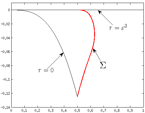
Figure 5: The boundary of the bipodal phase in the $(\varepsilon,\tau-\varepsilon^{3})$ coordinate. The part of phase boundary on which $\ddot{S}=0$ is shown in the thick red line. Note how this line is tangent to the ER curve at the triple point, as required by Theorem 4.1.

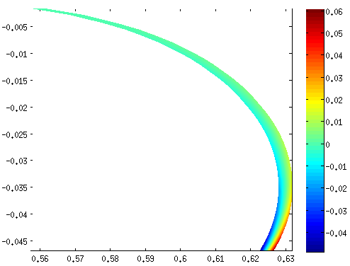
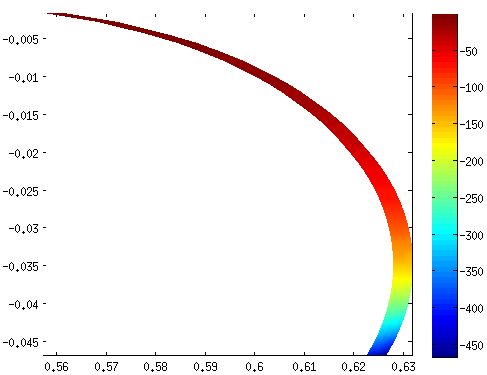
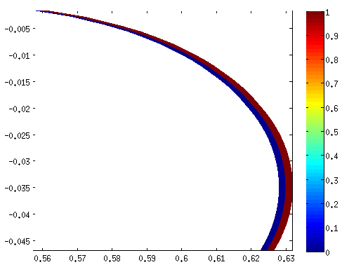
Figure 6: The function $\ddot{S}$ (top left), $\operatorname{sgn}(S)$ (bottom left), $\ddddot{S}$ (top right) and $\operatorname{sgn}(\ddddot{S})$ (bottom right) in the neighborhood of the phase transition curve $\Sigma$.

In Figure 6, we show the values of $\ddot{S}$ and $\ddddot{S}$ along a tube along the phase transition curve $\Sigma$. The plot is again in the $(\varepsilon,\tau-\varepsilon^{3})$ coordinate. To better visualize the transition, we visualize the function $\operatorname{sgn}(\ddot{S})$ and $\operatorname{sgn}(\ddddot{S})$ where $\operatorname{sgn}$ is the sign function: $\operatorname{sgn}(x)=1$ when $x\geq 0$ and $\operatorname{sgn}(x)=-1$ when $x<0$. The function $\dfrac{\partial\ddot{S}}{\partial\varepsilon}$ is show in Figure 7 along the phase transition curve $\Sigma$.

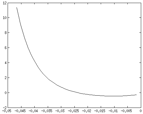
Figure 7: The plot of $\dfrac{\partial\ddot{S}}{\partial\varepsilon}$ on the curve $\Sigma$, i.e. as a function of $\tau-\varepsilon^{3}$.

The point is that $\ddddot{S}$ is always negative when $\ddot{S}=0$. Near the transition, we should thus expect optimizing graphons to have $|c-\frac{1}{2}|\approx\sqrt{-6\ddot{S}(\frac{1}{2})/\ddddot{S}(\frac{1}{2})}$ when $\ddot{S}(\frac{1}{2})>0$, and to have $c=\frac{1}{2}$ when $\ddot{S}(\frac{1}{2})<0$. In the next section we confirm this prediction with direct sampling of graphons.

6 Comparison to numerical sampling

In this section, we perform some numerical simulations using the sampling algorithm we developed in [16], and compare them to the results of the perturbation analysis. The sampling algorithm construct random samples of values of $\mathcal{S}$ in the parameter space graphons, and then take the maximum of the sampled values. This sampling algorithm is extremely expensive computationally, but when sufficiently large sample size are reached, we can achieve desired accuracy; see the discussions in [16]. We emphasize that our sampling algorithm does not assume bipodality of the maximizing graphons. In fact, we always start with the assumption that the graphons are $16$-podal. Bipodal structures are found when all the other clusters have size zero.

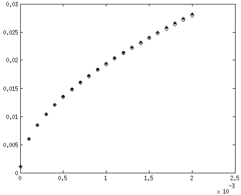
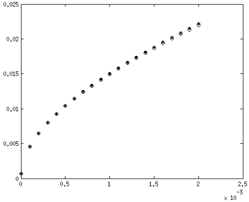
Figure 8: Comparison between the curve $(\varepsilon,|c-\frac{1}{2}|)$ (in $\circ$, given by the sampling algorithm) and $(\varepsilon,\sqrt{-6\ddot{S}(\frac{1}{2})/\ddddot{S}(\frac{1}{2})})$ (in $*$, given by the perturbation calculation) at two different $\tau-\varepsilon^{3}$ values: $-0.0348$ (left), $-0.0300$ (right).

In Figure 8, we plot the values of $|c-\frac{1}{2}|$ for optimizing graphons (found with the numerical sampling algorithm) and the real part of $\sqrt{-6\ddot{S}(\frac{1}{2})/\ddddot{S}(\frac{1}{2})}$ (given by the perturbation analysis) as functions of $\varepsilon$ along at two different $\tau-\varepsilon^{3}$ values. It is easily seen that the perturbation calculation gives very good fit when we are reasonably close to the phase transition curve $\Sigma$, but starts to be less accurate when we go farther out. A similar plot for the corresponding values of $a$, $b$, and $d$ are shown in Figure 9. As expected, $a$ and $d$ show square root singularities, just like $c$, but $b$ does not.

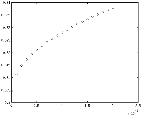
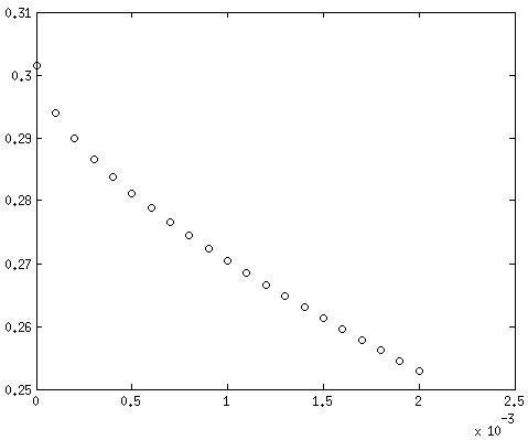
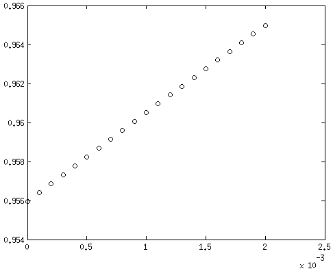
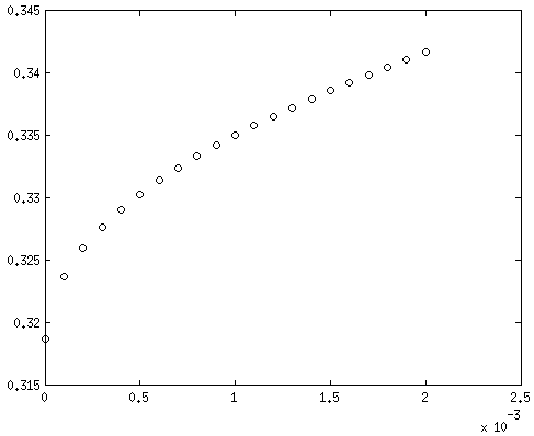
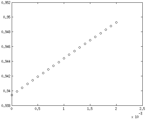
Figure 9: The plots of $a$ (left), $b$ (middle) and $d$ (right) versus $\varepsilon-\varepsilon_{0}$ at two different values of $\tau$: $0.2147$ (top row) and $0.2184$ (bottom row).

Finally, we show in Figure 10 some typical graphons that we obtained using the sampling algorithm. We emphasize again that in the sampling algorithm, we did not assume bipodality of the optimizing graphons. The numerics indicate that the optimizing graphons are really bipodal close to (on both sides) the phase transition curve $\Sigma$. These serve as numerical evidence to justify the perturbation calculations in this work.

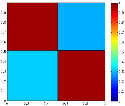
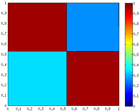
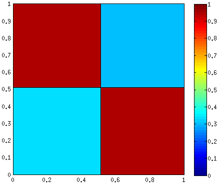
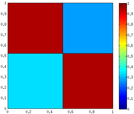
Figure 10: Typical graphons at points close to the phase boundary. The values of $(\varepsilon,\tau)$ are (from top left to bottom right): $(0.6299,0.2147)$, $(0.6315,0.2147)$, $(0.6290,0.2184)$ and $(0.6306,0.2184)$.

7 Conclusion

Our analysis began with the assumption that all entropy optimizers for relevant constraint parameters are multipodal; in fact bipodal, but we emphasize the more general feature. Multipodality is a fundamental aspect of the asymptotics of constrained graphs. It is the embodiment of phase emergence: the set of graphs with fixed constraints develops (“emerges into”) a well-defined global state as the number of nodes diverges, by partitioning the set of all nodes into a finite (usually small) number of equivalent parts, $\{P_{1},P_{2},\ldots\}$, of relative sizes $c_{j}$, and uniform (i.e. constant) probability $p_{ij}$ of an edge between nodes in $P_{i}$ and $P_{j}$. This unexpected fact has been seen in all simulations, and was actually proven throughout the phase spaces of edge/$k$-star models [5] and in particular regions of a wide class of models [6]. In this paper we are taking this as given, for a certain region of the edge/triangle phase space; we are assuming that our large constrained graphs emerge into such global states, and not just multipodal states but bipodal states, in accordance with simulation of the relevant constraint values in this model.

We analyzed the specific constraints of edge density approximately $1/2$ and triangle density less than $1/8$, and drew a variety of conclusions. First we used the facts, proven in [16], that there is a smooth curve in the phase space, indicated in Figure 1, such that: (i) to the left of the curve the (reduced) entropy optimizer is unique and is given by (2); (ii) the entropy optimizer is also unique to the right of the curve but is no longer symmetric. The curve thus represents a boundary between distinct phases of different symmetry. These facts were established in [16]. The analysis in this paper concerns the details of this transition. Here we want to speak to the significance of the results, in terms of symmetry breaking.

We take the viewpoint that the global states for these constraint values are sitting in a 4 dimensional space given by $a,b,d$ and $c$, quantities which describe the laws of interaction of the elements of the parts $P_{j}$ into which the node set is partitioned. (The notion of ‘vertex type’ has been introduced and analyzed in [7] and is useful in more general contexts.)

The symmetry $c_{1}=c_{2}=1/2$ and $a=b$ is therefore a symmetry of the rules by which the global state is produced. Each part $P_{j}$ into which the set of nodes is partitioned can be thought of as embodying the symmetry between the nodes it contains, but the symmetry of the global states is a higher-level symmetry, between the way these equivalence classes $P_{j}$ are connected. In this way the transition studied in this paper is an analogue of the symmetry-breaking fluid/crystal transition studied in the statistical analysis of matter in thermal equilibrium [22].

One consequence is a contribution to the old problem concerning the fluid/crystal transition. It has been known experimentally since the work of PW Bridgman in the early twentieth century that no matter how one varies the thermodynamic parameters (say mass and energy density) between fluid and crystal phases one must go through a singularity or phase transition. An influential theoretical analysis by L. Landau attributed this basic fact to the difference in symmetry between the crystal and fluid states, but this argument has never been completely convincing [14]. In our model this fact follows for phases $II$ and $III$ from the two-step process of first simplifying the space of global states to a finite dimensional space (of interaction rules) and then realizing the symmetry as acting in that space; it is then immediate that phases with different symmetry cannot be linked by a smooth (analytic) curve. This is one straightforward consequence of the powerful advantage of understanding our global states as multipodal, when compared say with equilibrium statistical mechanics.

References

- [1] C. Borgs, J. Chayes and L. Lovász, Moments of two-variable functions and the uniqueness of graph limits, Geom. Funct. Anal. 19 (2010) 1597-1619.
- [2] C. Borgs, J. Chayes, L. Lovász, V.T. Sós and K. Vesztergombi, Convergent graph sequences I: subgraph frequencies, metric properties, and testing, Adv. Math. 219 (2008) 1801-1851.
- [3] S. Chatterjee and P. Diaconis, Estimating and understanding exponential random graph models, Ann. Statist. 41 (2013) 2428-2461.
- [4] S. Chatterjee and S. R. S. Varadhan, The large deviation principle for the Erdős-Rényi random graph, Eur. J. Comb., 32 (2011), pp. 1000-1017.
- [5] R. Kenyon, C. Radin, K. Ren, and L. Sadun, Multipodal structures and phase transitions in large constrained graphs, arXiv:1405.0599, (2014).
- [6] R. Kenyon, C. Radin, K. Ren and L. Sadun, Bipodal structure in oversaturated random graphs, arXiv:1509.05370v1, (2015)
- [7] H. Koch, Vertex order in some large constrained random graphs, mparc 16-14, (2016)
- [8] L. Lovász and B. Szegedy, Limits of dense graph sequences, J. Combin. Theory Ser. B 98 (2006) 933-957.
- [9] L. Lovász and B. Szegedy, Szemerédi’s lemma for the analyst, GAFA 17 (2007) 252-270.
- [10] L. Lovász and B. Szegedy, Finitely forcible graphons, J. Combin. Theory Ser. B 101 (2011) 269-301.
- [11] L. Lovász, Large Networks and Graph Limits, American Mathematical Society, Providence, 2012.
- [12] M.E.J. Newman, Networks: an Introduction, Oxford University Press, 2010.
- [13] J. Park and M.E.J. Newman, Solution for the properties of a clustered network, Phys. Rev. E 72 (2005) 026136.
- [14] A. Pippard, The Elements of Classical Thermodynamics, Cambridge University Press, Cambridge, 1979, p. 122.
- [15] C. Radin, Phases in large combinatorial systems, arXiv:1601.04787v2 .
- [16] C. Radin, K. Ren and L. Sadun, The asymptotics of large constrained graphs, J. Phys. A: Math. Theor. 47 (2014) 175001.
- [17] C. Radin and L. Sadun, Phase transitions in a complex network, J. Phys. A: Math. Theor. 46 (2013) 305002.
- [18] C. Radin and L. Sadun, Singularities in the entropy of asymptotically large simple graphs, J. Stat. Phys. 158 (2015) 853-865.
- [19] A. Razborov, On the minimal density of triangles in graphs, Combin. Probab. Comput. 17 (2008) 603-618.
- [20] C. Radin and M. Yin, Phase transitions in exponential random graphs, Ann. Appl. Probab. 23(2013) 2458-2471.
- [21] D. Ruelle, Correlation functionals, J. Math. Phys. 6 (1965) 201–220.
- [22] D. Ruelle, Statistical Mechanics; Rigorous Results, Benjamin, New York, 1969.