Fault-tolerance of balanced hypercubes with faulty vertices and faulty edges

Abstract Let $F_{v}$ (resp. $F_{e}$) be the set of faulty vertices (resp. faulty edges) in the $n$-dimensional balanced hypercube $BH_{n}$. Fault-tolerant Hamiltonian laceability in $BH_{n}$ with at most $2n-2$ faulty edges is obtained in [Inform. Sci. 300 (2015) 20–27]. The existence of edge-Hamiltonian cycles in $BH_{n}-F_{e}$ for $|F_{e}|\leq 2n-2$ are gotten in [Appl. Math. Comput. 244 (2014) 447–456]. Up to now, almost all results about fault-tolerance in $BH_{n}$ with only faulty vertices or only faulty edges. In this paper, we consider fault-tolerant cycle embedding of $BH_{n}$ with both faulty vertices and faulty edges, and prove that there exists a fault-free cycle of length $2^{2n}-2|F_{v}|$ in $BH_{n}$ with $|F_{v}|+|F_{e}|\leq 2n-2$ and $|F_{v}|\leq n-1$ for $n\geq 2$. Since $BH_{n}$ is a bipartite graph with two partite sets of equal size, the cycle of a length $2^{2n}-2|F_{v}|$ is the longest in the worst-case.

Keywords Balanced hypercube; Cycle embedding; Fault tolerance; Interconnection network.

1 Introduction

In a multiprocessor system, processors communicate by exchanging messages through an interconnection network whose topology often modeled by an undirected graph $G=(V,E)$, where every vertices in $V$ corresponds to a processor, and every edge in $E$ corresponds to a communication link.

The $n$-dimensional balanced hypercube $BH_{n}$, proposed by Wu and Huang [16], is an important class of generalizations of the popular hypercube interconnection network for parallel computing. It has many desirable properties, such as bipartite, regularity, recursive structure, vertex-transitive [10] and edge transitive [25], as the hypercube. However, the balanced hypercube is superior to the hypercube in a sense that it has a smaller diameter than that of the hypercube and supports an efficient reconfiguration without changing the adjacent relationship among tasks [16]. More desired properties of balanced hypercubes have been shown in the literature. Let $BH_{n}$ be an $n$-dimensional balanced hypercube. Wu and Huang [10] proved that $BH_{n}$ is bipartite graph and vertex transitive. Huang and Wu [11] studied resource placement problem in $BH_{n}$. Zhou et al. [25] obtained that $BH_{n}$ is edge transitive and determined the cyclic connectivity and cyclic edge-connectivity of $BH_{n}$. Xu et al. [18] showed that $BH_{n}$ is edge-pancyclic and Hamiltonian laceable. Yang [19] further showed that $BH_{n}$ is bipanconnected for all $n\geq 1$. Yang [20] determined super connectivity and super edge connectivity of $BH_{n}$. Yang [21] also gave the conditional diagnosability of $BH_{n}$ under the PMC model. Lü et al. [13] obtained (conditional) matching preclusion number of $BH_{n}$. Lü and Zhang [14] further proved that $BH_{n}$ is hyper-Hamiltonian laceable. Cheng et al. [5] showed that there exist two vertex-disjoint path cover in $BH_{n}$.

Since faulty vertices and faulty edges may happen in the real world networks, the fault-tolerant of networks has been proposed, see [7, 9, 15, 17, 24] etc.. There are some results about the fault-tolerance of $BH_{n}$. Let $F_{v}$ (resp. $F_{e}$) be the set of faulty vertices (resp. faulty edges) in the $n$-dimensional balanced hypercube $BH_{n}$. As examples, Zhou et al. [26] derived that $BH_{n}$ is $(2n-2)$-edge-fault Hamiltonian laceable for $n\geq 2$, i.e., if at most $2n-2$ faulty edges occurs, the resulting graph remains Hamiltonian laceable. Cheng et al. in [4] proved that if $|F_{v}|\leq n-1$ faulty vertices occurs, every fault-free edge of $BH_{n}-F_{v}$ lies on a fault-free cycle of every even length from $4$ to $2^{2n}-2|F_{v}|$. Cheng et al. in [3] derived that $BH_{n}$ is $(2n-3)$-edge-fault-bipancyclic, that is, there are at most $|F_{e}|\leq 2n-3$ faulty edges, every fault-free edge of $BH_{n}-F_{e}$ lies on a fault-free cycle of every even length from $4$ to $2^{2n}$. Hao et al. [8] gave the existence of $(2n-2)$- edge-fault-tolerant cycle embedding in $BH_{n}$. But up to now, almost all results about fault-tolerance in $BH_{n}$ with only faulty vertices or only faulty edges.

In this paper, we consider cycle embedding of $BH_{n}$ with both faulty vertices and faulty edges, and prove that there exists a fault-free cycle of length $2^{2n}-2|F_{v}|$ in $BH_{n}$ with $|F_{v}|+|F_{e}|\leq 2n-2$ and $|F_{v}|\leq n-1$ for $n\geq 2$. Since $BH_{n}$ is a bipartite graph with two partite sets of equal size, the cycle of length $2^{2n}-2|F_{v}|$ is the longest in the worst-case. This paper improves the results about the longest fault-free cycle in $BH_{n}$ with only faulty vertices or only faulty edges.

The rest of this paper is organized as follows. Section 2 presents some necessary definitions of graphs and properties of balanced hypercubes as preliminaries. The proof of our main result is given in Section 3. Section 4 concludes this paper.

2 Preliminaries

Let $G=(V,E)$ be a simple undirected graph, where $V$ is the vertex-set of $G$ and $E$ is the edge set of $G$. The neighborhood of a vertex $u$ in $G$ is the set of all vertices adjacent to $u$ in $V(G)$, denoted by $N_{G}(u)$. The cardinality $|N_{G}(u)|$ represents the degree of $u$ in $G$, denoted by $d_{G}(u)$. A path $P$, denoted by $P=\langle u_{0},u_{1},\ldots,u_{k}\rangle$, is a sequence of vertices where two successive vertices are adjacent in $G$. $u_{0}$ and $u_{k}$ are called the end-vertices of a path $P$. A $u-v$ path which is denoted by $P[u,v]$ is a path with endpoints $u$ and $v$. For $0\leq i<j\leq k$, let $P=\langle u_{0},u_{1},\ldots,u_{k}\rangle=\langle u_{0},u_{1},\ldots,u_{i},P[u_{i},u_{j}],u_{j},\ldots,u_{k}\rangle$, where $P[u_{i},u_{j}]=\langle u_{i},u_{i+1},\ldots,u_{j}\rangle$. A cycle is a path that two ends are the same vertex. A cycle (resp. path) is a Hamiltonian cycle (resp. Hamiltonian path) if it traverses all the vertices of $G$ exactly once. The length of a path is the number of edges in it.

A graph $G$ is said to be Hamiltonian connected if there exists a Hamiltonian path between any two vertices of $G$. It is easy to see that any bipartite graph with at least three vertices is not Hamiltonian connected. A bipartite graph $G$ is Hamiltonian laceable (resp. strongly Hamiltonian laceable) if there exists a of length $|V(G)|-1$ (resp. $|V(G)|-2$) between two arbitrary vertices from different (resp. same) partite sets. A bipartite graph $G$ with bipartition $V_{0}\cup V_{1}$ is hyper-Hamiltonian laceable if it is Hamiltonian laceable and, for any vertex $v\in V_{i}$ ($i\in\{0,1\})$, there is a Hamiltonian path in $G-v$ between any pair of vertices in $V_{1-i}$.

An $n$-dimensional balanced hypercube, denoted by $BH_{n}$, is proposed by Wu and Huang [16] which is defined as an undirected simple graph.

Definition 2.1

An $n$-dimensional balanced hypercube $BH_{n}$ with $n\geq 1$ has $2^{2n}$ vertices with addresses $(a_{0},a_{1},\ldots,a_{n-1})$, where $a_{i}\in\{0,1,2,3\}$ for each $0\leq i\leq n-1$. Each vertex $(a_{0},a_{1},\ldots,a_{n-1})$ is adjacent to the following $2n$ vertices:

$$\left\{\begin{array}[]{l}((a_{0}\pm 1)({\rm mod}\ 4),a_{1},\ldots,a_{n-1});\\ ((a_{0}\pm 1)({\rm mod}\ 4),a_{1},\ldots,a_{j-1},(a_{j}+(-1)^{a_{0}})({\rm mod}\ 4),a_{j+1},\ldots,a_{n-1}),\end{array}\right.$$

where $j$ is an integer with $1\leq j\leq n-1$.

‘$+$’ and ‘$-$’ are the operation with $``({\rm mod}\ 4)"$. For notation convenience, $``({\rm mod}\ 4)"$ is omitted. The balanced hypercube $BH_{n}$ can also be recursively defined.

Definition 2.2

$BH_{n}$ can be recursively constructed as follows:

1. $BH_{1}$ is a cycle consisting of $4$ vertices labeled as $0,1,2,3$ respectively.

2. For $n\geq 2$, $BH_{n}$ consists of four copies of $BH_{n-1}$, denoted by $BH_{n-1}^{i}$ for each $i\in\{0,1,2,3\}$. Each vertex $(a_{0},a_{1},\ldots,a_{n-2},i)$ in $BH_{n-1}^{i}$ has two extra adjacent vertices which are also called extra neighbors:

   1. $(a_{0}\pm 1,a_{1},\ldots,a_{n-2},i+1)$ in $BH_{n-1}^{i+1}$ if $a_{0}$ is even.

   2. $(a_{0}\pm 1,a_{1},\ldots,a_{n-2},i-1)$ in $BH_{n-1}^{i-1}$ if $a_{0}$ is odd.

$BH_{1}$ and $BH_{2}$ are illustrated in Figure 1.

Figure 1: $BH_{1}$ and $BH_{2}$

The first element $a_{0}$ of vertex $(a_{0},a_{1},\ldots,a_{n-2},a_{n-1})$ is called the inner index, and the other elements $a_{i}$, for all $1\leq i\leq n-1$, are called $i$-dimensional index. By [23, Lemma 5], for each vertex $u$ of $BH_{n}$, there exists a unique vertex, denoted by $u^{\ast}$, such that $N_{BH_{n}}(u)=N_{BH_{n}}(u^{\ast})$.

Since $BH_{n}$ is a bipartite graph, we refer to a vertex with an odd inner index as a black vertex and a vertex with an even inner index as a white vertex. If two adjacent vertices $u$ and $v$ differ in only the inner index, the edge $e=(u,v)$ is said to be $0$-dimensional and $v$ is a $0$-dimensional neighbor of $u$. Let $[n]=\{0,1,\ldots,n-1\}$ (but not general meaning $\{1,2,\ldots,n\}$). Likewise if two adjacent vertices $u$ and $v$ not only differ in the inner index, but also differ in some $j$-dimensional index ($j\in[n]$), the edge $e=(u,v)$ is said to be $j$-dimensional, and $v$ is the $j$-dimensional neighbor of $u$. Let $E_{j}$, where $j\in[n]$, denote the set of all $j$-dimensional edges. For $i\in\{0,1,2,3\}$ and $j\in[n]$, we use $BH_{n-1}^{j,i}$ to denote $(n-1)$-dimensional sub-balanced hypercubes of the $BH_{n}$ induced by all vertices labeled by $(a_{0},a_{1},\ldots,a_{j-1},i,a_{j+1},\ldots,a_{n-2},a_{n-1})$. Obviously, $BH_{n}-E_{j}=\bigcup\limits_{i=0}^{3}BH_{n-1}^{j,i}$ and $BH_{n-1}^{j,i}\cong BH_{n-1}$. The edges between $BH_{n-1}^{j,i}$ and $BH_{n-1}^{j,i+1}$ are called $j$-dimensional crossing edges, where $i\in\{0,1,2,3\}$ and $j\in\{1,2,\ldots,n-1\}$. If $j=n-1$, $BH_{n-1}^{j,i}$ and $E_{j}$ are denoted by $BH_{n-1}^{i}$ and $E_{c}$, respectively, where $i\in\{0,1,2,3\}$ and $(n-1)$-dimension crossing edges are called crossing edges. Let $E_{0}$ be the set of all $0$-dimensional edges, Lü et al. [13] obtained that $BH_{n}-E_{0}$ has four components, each component is isomorphic to $BH_{n-1}$.

Some known basic properties of $BH_{n}$ are given as follows.

Lemma 2.3

([16]) The balanced hypercube $BH_{n}$ is bipartite and vertex transitive.

Lemma 2.4

([25]) The balanced hypercube $BH_{n}$ is edge transitive.

Lemma 2.5

([18]) The balanced hypercube $BH_{n}$ is edge-bipancyclic and Hamiltonian laceable for all $n\geq 1$.

Lemma 2.6

([19]) The balanced hypercube $BH_{n}$ is bipanconnected for all $n\geq 1$.

Lemma 2.7

([14]) The balanced hypercube $BH_{n}$ is hyper-Hamiltonian laceable for $n\geq 1$. Thus, $BH_{n}$ is strongly Hamiltonian laceability.

Lemma 2.8

([5]) Let $X$ and $Y$ be two distinct partite sets of $BH_{n}$. Assume $u$ and $x$ are two different vertices in $X$, $v$ and $y$ are two different vertices in $Y$. Then there exist two vertex-disjoint paths $P[x,y]$ and $R[u,v]$, and $V(P[x,y])\cup V(R[u,v])=V(BH_{n})$.

Lemma 2.9

1. ([18]) Let $e=(u,v)$ be an edge of $BH_{n}$. $e$ is contained in a cycle $C$ of length $8$ in $BH_{n}$ such that $|E(C)\cap E(BH_{n-1}^{i})|=1$, where $i=0,1,2,3$.

2. ([4]) Let $e=(u,v)$ be an edge of $BH_{n}$. If $e$ is along dimension $j$ ($1\leq j\leq n-1$), then there are $2n-2$ internal vertex-disjoint paths of length $7$ joining $u$ and $v$ such that each path has only one edge in each $BH_{n-1}^{j,i}$, where $i\in\{0,1,2,3\}$.

3. ([4]) Let $e=(x,y)$ be any edge in $BH_{n-1}^{j,0}$, then there exist two internal vertex-disjoint paths $\langle x,y_{1},x_{1},y_{2},x_{2},y_{3},x_{3},y\rangle$ and $\langle x,y_{1}^{\prime},x_{1}^{\prime},y_{2}^{\prime},x_{2}^{\prime},\\ y_{3}^{\prime},x_{3}^{\prime},y\rangle$ in $BH_{n}$ such that $(x_{i},y_{i}),(x_{i}^{\prime},y_{i}^{\prime})\in E(BH_{n-1}^{j,i})$, where $1\leq j\leq n-1$ and $i=1,2,3$.

Lemma 2.10

([8]) Let $A=\{e_{1},e_{2},\ldots,e_{k}\}$ for $k\geq 2$ be the set of $j$-dimensional edges in $BH_{n-1}^{i}$, where $j\in[n]$ and $i\in\{0,1,2,3\}$. Then there are cycles $D_{1},D_{2},\ldots,D_{k}$ which contain $e_{1},e_{2},\ldots,e_{k}$, respectively, such that the length of each cycle is $8$, $D_{1},D_{2},\ldots,D_{k}$ are edge disjoint and $|E(D_{m})\cap E(BH_{n-1}^{t})|=1$ for every $m\in\{1,2,\ldots,k\}$ and $t\in\{0,1,2,3\}$. Moreover, for any $i,j\in[k]$, if $e_{i}\cap e_{j}=\emptyset$, then $D_{i},D_{j}$ are also vertex-disjoint. If $e_{i}\cap e_{j}=\{u\}$, then $D_{i},D_{j}$ are vertex-disjoint except a vertex $u$.

For the fault tolerance of $BH_{n}$, Cheng et al. [3] and [4] derived the following two results, respectively..

Lemma 2.11

([3]) Let $F_{e}$ be the set of faulty vertices in $BH_{n}$ with $|F_{e}|\leq 2n-3$. Then every fault-free edge of $BH_{n}-F_{e}$ lies on a fault-free cycle of every even length from $4$ to $2^{2n}$ inclusive, where $n\geq 2$.

Lemma 2.12

([4]) Let $F_{v}$ be the set of faulty vertices in $BH_{n}$ with $|F_{v}|\leq n-1$. Then every fault-free edge of $BH_{n}-F_{v}$ lies on a fault-free cycle of every even length from $4$ to $2^{2n}-2|F_{v}|$ inclusive, where $n\geq 1$.

Hao et al. [8] and Zhou et al. [26] obtained the following two results, respectively.

Lemma 2.13

([8]) Let $F_{e}$ be a faulty edge set of the balanced hypercube $BH_{n}$ with $|F_{e}|\leq 2n-2$, $n\geq 1$, then there exists a fault-free Hamiltonian path between any two adjacent vertices $x$ and $y$ in $BH_{n}$.

Lemma 2.14

([26]) $BH_{n}$ is $(2n-2)$-edge-fault Hamiltonian laceable for $n\geq 2$.

3 Main results

In this section, we consider cycle embedding in faulty balanced hypercube $BH_{n}$. For this purpose, we need the following lemma.

Lemma 3.1

Let $F_{v}$ (resp. $F_{e}$) be the set of faulty vertices (resp. faulty edges) with $|F_{v}|+|F_{e}|\leq n-1$ in $BH_{n}$ for $n\geq 1$. Then, there is a fault-free path in $BH_{n}$ whose length is $2^{2n}-2|F_{v}|-1$ between any two adjacent vertices $x$ and $y$ in $BH_{n}$.

Proof. Assume $x$ is a white vertex and $y$ is a black vertex and $(x,y)\in E(BH_{n})$. Recall that $f_{e}=|F_{e}|$, $f_{v}=|F_{v}|$, $f=f_{e}+f_{v}$. We only need to prove the result holds for $f=n-1$. We show the lemma by induction on $n$. If $n=1$, $f=0$, $BH_{1}$ is a cycle of length $4$, so the result is right. Now we consider $n=2$. If $f_{e}=0$, then $f_{v}=1$. Since $x$ and $y$ are adjacent, regard $(x,y)$ as a fault-free edge, by Lemma 2.12, the edge $(x,y)$ lies in a fault-free cycle of length $2^{4}-2$, this implies there exists a fault-free path $P[x,y]$ of length $2^{4}-2-1=13$. If $f_{v}=0$, then $f_{e}=1$. Since $x$ and $y$ are adjacent, by Lemma 2.13, there exists a fault-free Hamiltonian $x-y$ path of length $2^{4}-1=15$. The lemma holds for $n=2$.

Assume that the lemma holds for $BH_{n-1}$ for $n\geq 3$. Now we consider $BH_{n}$. If $BH_{n}$ has no faulty edges, then $f_{v}\leq n-1$. By Lemma 2.12, there exists a fault-free path of length $2^{2n}-2f_{v}-1$ between $x$ and $y$. So we assume that there is at least one faulty edge. Without loss of generality, suppose there exists an $(n-1)$-dimensional faulty edge. We can divide $BH_{n}$ into $BH_{n-1}^{i}$, $i=0,1,2,3$, along $(n-1)$-dimension. For $i\in\{0,1,2,3\}$, let $f_{e}^{i}=|F_{e}\cap E(BH_{n-1}^{i})|$ and $f_{v}^{i}=|F_{v}\cap V(BH_{n-1}^{i})|$. Moreover, we have that $0\leq f_{e}^{i}+f_{v}^{i}\leq n-2$ for each $i\in\{0,1,2,3\}$. There are the following two cases.

Case 1. $x$ and $y$ are in the same $BH_{n-1}^{i}$ for some $i\in\{0,1,2,3\}$. Without loss of generality, let $i=0$.

By the inductive hypothesis, there exists a fault-free $x-y$ path $P_{0}$ in $BH_{n-1}^{0}$ of length $2^{2(n-1)}-2f_{v}^{0}-1$. We claim that there exists at least one $k\in\{0,1,\ldots,n-2\}$ such that $P_{0}$ contains at least $2n-1$ $k$-dimensional edges. Otherwise, for every $k\in\{0,1,\ldots,n-2\}$, $P_{0}$ contains at most $2n-2$ $k$-dimensional edges. As a result, $P_{0}$ contains at most $(n-1)(2n-2)$ edges. Since $|P_{0}|=2^{2(n-1)}-2f_{v}^{0}-1\geq 2^{2(n-1)}-2n+1>(n-1)(2n-2)$ for $n\geq 3$, it is a contradiction. Since $f=n-1\leq 2n-1$ for $n\geq 3$, by Lemma 2.10, we can find a $k$-dimensional edge $(u_{0},v_{0})$ (assume $u_{0}$ is white, $v_{0}$ is black) on $P_{0}$, such that $(u_{0},v_{0})$ is contained in a fault-free $8$-cycle $C$, say $C=\langle u_{0},v_{0},u_{3},v_{3},u_{2},v_{2},u_{1},v_{1},u_{0}\rangle$, where $(u_{i},v_{i})\in E(BH_{n-1}^{i})$ for $i\in\{0,1,2,3\}$.

By the inductive hypothesis in $BH_{n-1}^{i}$, for each $i\in\{1,2,3\}$, there exists a fault-free $u_{i}-v_{i}$ path $P_{i}$ in $BH_{n-1}^{i}$ of length $2^{2(n-1)}-2f_{v}^{i}-1$. Therefore, $\langle x,P[x,u_{0}],u_{0},v_{1},P_{1},u_{1},v_{2},P_{2},\\ u_{2},v_{3},P_{3},u_{3},v_{0},P[v_{0},y],y\rangle$ is a desired fault-free $x-y$ path in $BH_{n}$ of length $\Sigma_{i=0}^{3}(2^{2(n-1)}-2f_{v}^{i}-1)+3=2^{2n}-2f_{v}-1$.

Case 2. $x$ and $y$ are in two distinct $BH_{n-1}^{i}$’s, where $i\in\{0,1,2,3\}=[4]$.

Without loss of generality, suppose $x\in V(BH_{n-1}^{0})$. Since $x$ and $y$ are adjacent, $y\in V(BH_{n-1}^{1})$. By Lemma 2.9(2) and $f\leq n-1\leq 2n-2$ for $n\geq 3$, there exists a fault-free $x-y$ path $P$, say $P=\langle x,v_{0},u_{3},v_{3},u_{2},v_{2},u_{1},y\rangle$, of length $7$ such that $P$ has only one edge in $BH_{n-1}^{i}$ for each $i=0,1,2,3$. By the inductive hypothesis, there exists a fault-free $x-v_{0}$ (resp. $u_{3}-v_{3}$, $u_{2}-v_{2}$ and $u_{1}-y$) path $P_{0}$ (resp. $P_{3}$, $P_{2}$ and $P_{1}$) in $BH_{n-1}^{0}$ (resp. $BH_{n-1}^{3}$, $BH_{n-1}^{2}$ and $BH_{n-1}^{1}$) of length $2^{2(n-1)}-2f_{v}^{0}-1$ (resp. $2^{2(n-1)}-2f_{v}^{3}-1$, $2^{2(n-1)}-2f_{v}^{2}-1$ and $2^{2(n-1)}-2f_{v}^{1}-1$). A fault-free $x-y$ path of $BH_{n}$ can be constructed as $\langle x,P_{0},v_{0},u_{3},P_{3},v_{3},u_{2},P_{2},v_{2},u_{1},P_{1},y\rangle$ of length $\Sigma_{i=0}^{3}(2^{2(n-1)}-2f_{v}^{i}-1)+3=2^{2n}-2f_{v}-1$.

By the above cases, the proof is complete.

Lemma 3.2

Let $v$ be a faulty vertex and $e$ be a faulty edge in $BH_{2}$. Then there exists a fault-free cycle of length $14$ in $BH_{2}$.

Proof. By Lemma 2.4, $BH_{2}$ is edge transitive, we may assume that $a=((0,0),(1,1))$ is a faulty edge. For each possible faulty vertex $v\in V(BH_{2})$, we can find a desired cycle. All the cases are listed in Table 1.

$v=(0,0)$ or $(1,0)$

$\langle(3,0),(2,0),(3,1),(0,1),(1,1),(2,1),(1,2),(2,2),(3,2),(0,2),(1,3),(2,3),(3,3),(0,3),(3,0)\rangle$

$v=(3,0)$ or $(2,0)$

$\langle(0,0),(1,0),(0,3),(3,3),(2,3),(1,3),(0,2),(3,2),(2,2),(1,2),(2,1),(1,1),(0,1),(3,1),(0,0)\rangle$

$v=(0,1)$ or $(1,1)$

$\langle(0,0),(1,0),(2,0),(3,1),(2,1),(1,2),(2,2),(3,2),(0,2),(1,3),(2,3),(3,3),(0,3),(3,0),(0,0)\rangle$

$v=(3,1)$ or $(2,1)$

$\langle(0,0),(1,0),(2,0),(1,1),(0,1),(3,2),(2,2),(1,2),(0,2),(1,3),(2,3),(3,3),(0,3),(3,0),(0,0)\rangle$

$v=(0,3)$ or $(1,3)$

$\langle(0,0),(3,0),(2,0),(1,0),(2,3),(3,3),(2,2),(3,2),(0,2),(1,2),(2,1),(1,1),(0,1),(3,1),(0,0)\rangle$

$v=(3,3)$ or $(2,3)$

$\langle(0,0),(3,0),(2,0),(1,0),(0,3),(1,3),(0,2),(3,2),(2,2),(1,2),(2,1),(1,1),(0,1),(3,1),(0,0)\rangle$

$v=(0,2)$ or $(1,2)$

$\langle(0,0),(1,0),(2,0),(3,0),(0,3),(3,3),(2,3),(1,3),(2,2),(3,2),(0,1),(1,1),(2,1),(3,1),(0,0)\rangle$

$v=(3,2)$ or $(2,2)$

$\langle(0,0),(1,0),(2,0),(3,0),(0,3),(3,3),(2,3),(1,3),(0,2),(1,2),(2,1),(1,1),(0,1),(3,1),(0,0)\rangle$

Table 1: Desired cycles of length $14$ in $BH_{2}$ with a faulty vertex $v$ and a faulty edge ((0,0),(1,1))

The following is our main result.

Theorem 3.3

Let $F_{v}$ and $F_{e}$ be the set of faulty vertices and faulty edges, respectively, with $|F_{v}|\leq n-1$ and $|F_{v}|+|F_{e}|\leq 2n-2$ in $BH_{n}$, where $n\geq 2$. Then there exists a fault-free cycle of length $2^{2n}-2|F_{v}|$ in $BH_{n}$.

Proof. We prove this theorem by induction on $n$. Recall that $E_{j}$ is the set of $j$-dimensional edges in $BH_{n}$ for $j\in[n]$. Since $|F_{v}|+|F_{e}|\leq 2n-2$, there exists a $j\in[n]$ such that $|F_{e}\cap E_{j}|\leq 1$. Without loss of generality, let $j=n-1$. Then we can divide $BH_{n}$ into four components, say $BH_{n-1}^{i}$, $i=0,1,2,3$, along $(n-1)$-dimension. Let $F_{c}=F_{e}\cap E_{n-1}$, then $f_{c}=|F_{c}|\leq 1$. Recall that $f_{v}=|F_{v}|$, $f_{e}=|F_{e}|$, $f=f_{v}+f_{e}$, $f_{e}^{i}=|F_{e}\cap E(BH_{n-1}^{i})|$ and $f_{v}^{i}=|F_{v}\cap V(BH_{n-1}^{i})|$, so $f_{i}=f_{e}^{i}+f_{v}^{i}$ for $i\in\{0,1,2,3\}$.

If $n=2$, then $f_{v}+f_{e}\leq 2$ and $f_{v}\leq 1$. If $f_{v}=1$ and $f_{e}=0$, then by Lemma 2.12, the result is right. If $f_{v}=1$ and $f_{e}=1$, the result follows from Lemma 3.2. If $f_{v}=0$ and $f_{e}\leq 2$. Choose a fault-free edge $(u,v)$, by Lemma 2.13, there exists a fault-free Hamiltonian path $P$ between $u$ and $v$ in $BH_{2}$, then $\langle u,P,v,u\rangle$ is the desired cycle of $BH_{2}$. The theorem is true for $n=2$.

For $n\geq 3$, we assume that the theorem is true in $BH_{m}$ with $f_{v}+f_{e}\leq 2m-2$ and $f_{v}\leq m-1$ for every integer $2\leq m<n$. Now we consider $BH_{n}$ as follows. If $BH_{n}$ has no faulty vertices, then $f_{v}=0$ and $f_{e}\leq 2n-2$. Choose a fault-free edge $(x,y)$, since $f_{e}\leq 2n-2$, by Lemma 2.13, there exists a fault-free Hamiltonian path $P$ from $x$ to $y$ in $BH_{n}$. Let $C=\langle x,P,y,x\rangle$. Clearly, $|E(C)|=2^{2n}=2^{2n}-2f_{v}$. So we assume $1\leq f_{v}\leq n-1$ in the following. We only need to consider the following three cases.

Case 1. For each $i\in\{0,1,2,3\}$, $0\leq f_{i}\leq 2n-4$.

Subcase 1.1. For each $i\in\{0,1,2,3\}$, $0\leq f_{i}\leq n-2$.

By the inductive hypothesis, there exists a cycle $C_{0}$ in $BH_{n-1}^{0}$ of length $2^{2(n-1)}-2f_{v}^{0}$. Select an $(u_{0},v_{0})\in E(C_{0})$ and assume $u_{0}$ is white. By Lemma 2.9(3), since $f_{c}\leq 1$, $(u_{0},v_{0})$ is contained in two $8$-cycles which has only one common edge $(u_{0},v_{0})$, so we can find a $8$-cycle $C$, say $C=\langle u_{0},v_{0},u_{3},v_{3},u_{2},v_{2},u_{1},v_{1},u_{0}\rangle$, where $(u_{i},v_{i})\in E(BH_{n-1}^{i})$ for $i\in\{0,1,2,3\}$, such that the crossing edge $(u_{i},v_{i+1})$ for each $i\in\{0,1,2,3\}$ is fault-free, where $v_{4}=v_{0}$. Since $f_{i}\leq n-2$ and $BH_{n-1}^{i}\cong BH_{n-1}$ for $i\in\{1,2,3\}$, by Lemma 3.1, there exists a fault-free $u_{i}-v_{i}$ path $P_{i}$ of length $2^{2(n-1)}-2f_{v}^{i}-1$ in $BH_{n-1}^{i}$. Let $P_{0}=C_{0}-(u_{0},v_{0})$. So $\langle u_{0},v_{1},P_{1},u_{1},v_{2},P_{2},u_{2},v_{3},P_{3},u_{3},v_{0},\\ P_{0},u_{0}\rangle$ is a desired fault-free cycle in $BH_{n}$ of length $2^{2n}-2f_{v}$.

Subcase 1.2. There exists only one $i\in\{0,1,2,3\}$ such that $n-1\leq f_{i}\leq 2n-4$. Without loss of generality, let $i=0$. It implies that $0\leq f_{j}\leq n-2$ for all $j\in\{1,2,3\}$.

Subcase 1.2.1. $n-1\leq f_{0}\leq 2n-4$, $f_{v}^{0}\leq n-2$.

By the inductive hypothesis, there exists a fault-free cycle $C_{0}$ in $BH_{n-1}^{0}$ of length $2^{2(n-1)}-2f_{v}^{0}$. By the similar discussions as Case 1 in the proof of Lemma 3.1, we can find an edge $(u_{0},v_{0})$ (assume $u_{0}$ is white, $v_{0}$ is black) on $C_{0}$, such that $(u_{0},v_{0})$ is contained in a fault-free $8$-cycle $C$, say $C=\langle u_{0},v_{0},u_{3},v_{3},u_{2},v_{2},u_{1},v_{1},u_{0}\rangle$, where $(u_{i},v_{i})\in E(BH_{n-1}^{i})$ for $i\in\{1,2,3\}$. Since $0\leq f_{i}\leq n-2$ for $i\in\{1,2,3\}$, by Lemma 3.1 in $BH_{n-1}^{i}$, there exists a fault-free $u_{i}-v_{i}$ path $P_{i}$ in $BH_{n-1}^{i}$ of length $2^{2(n-1)}-2f_{v}^{i}-1$. Let $P_{0}=C_{0}-(u_{0},v_{0})$. Therefore, $\langle u_{0},v_{1},P_{1},u_{1},v_{2},P_{2},u_{2},v_{3},P_{3},u_{3},v_{0},P_{0},u_{0}\rangle$ is a desired fault-free cycle in $BH_{n}$ of length $2^{2n}-2f_{v}$.

Subcase 1.2.2. $n-1\leq f_{0}\leq 2n-4$, $f_{v}^{0}=n-1$.

It implies that $f_{v}^{j}=0$ and $f_{e}^{j}\leq f-f_{v}\leq n-1$ for each $j\in\{1,2,3\}$. We regard one faulty vertex in $BH_{n-1}^{0}$ as a fault-free vertex, so $f_{v}^{\prime}=f_{v}^{0}-1=f_{v}-1=n-2$. By the inductive hypothesis, there exists a cycle $C_{0}$ in $BH_{n-1}^{0}$ of length $2^{2(n-1)}-2f_{v}^{\prime}$, where $f_{v}^{\prime}=f_{v}^{0}-1$. Note that $C_{0}$ contains at most one faulty vertex.

If $C_{0}$ does not contain any faulty vertex, choose an edge, say $(u_{0},v_{0})\in E(C_{0})$ (assume $u_{0}$ is white, $v_{0}$ is black). By Lemma 2.9(3) and $f_{c}\leq 1$, $(u_{0},v_{0})$ is contained in a cycle $C$, say $C=\langle v_{0},u_{0},v_{1},u_{1},v_{2},u_{2},v_{3},u_{3},v_{0}\rangle$, of length $8$ in $BH_{n}$ such that $E(C)\cap E(BH_{n-1}^{i})=\{(u_{i},v_{i})\}$ and $(u_{i},v_{i+1})$ is fault-free for each $i\in\{0,1,2,3\}$. Since for any $i\in\{1,2\}$, $f_{v}^{i}=0$ and $f_{e}^{i}\leq n-1\leq 2n-2$ for $n\geq 3$, by Lemma 2.14, there exists a fault-free path $P_{i}$ between $u_{i}$ and $v_{i}$ in $BH_{n-1}^{i}$ whose length is $2^{2(n-1)}-1$. Since $f_{v}^{3}=0$ and $f_{e}^{3}\leq n-1\leq 2n-3$ for $n\geq 3$, by Lemma 2.11, there exists a fault-free cycle $C_{3}$ of length $2^{2(n-1)}-2$ passing through $(u_{3},v_{3})$. Let $P_{i}=C_{i}-(u_{i},v_{i})$ for $i=0,3$. A desired fault-free cycle of $BH_{n}$ can be constructed as $\langle u_{0},v_{1},P_{1},u_{1},v_{2},P_{2},u_{2},v_{3},P_{3},u_{3},v_{0},P_{0},u_{0}\rangle$ whose length is $2^{2(n-1)}-2(f_{v}^{0}-1)-1+2(2^{2(n-1)}-1)+(2^{2(n-1)}-3)+4=2^{2n}-2f_{v}^{0}=2^{2n}-2f_{v}$.

Now assume that $C_{0}$ contains one faulty vertex $u_{0}$ and $u_{0}$ is black. (If $C_{0}$ contains a white faulty vertex, the discussions are similar, so it is omitted.) Let $a_{0}$ and $b_{0}$ be two vertices adjacent to $u_{0}$ on $C_{0}$. Let $c_{0}\in C_{0}$ be a neighbor of $b_{0}$. Recall that each vertex has two extra neighbors and $f_{c}\leq 1$, we can choose the extra neighbors $c_{1}\in V(BH_{n-1}^{1})$ and $a_{3}\in V(BH_{n-1}^{3})$ of $a_{0}$ and $c_{0}$, respectively, such that both $(a_{0},c_{1})$ and $(c_{0},a_{3})$ are fault-free. For $i\in\{1,2\}$, let $(a_{i},c_{i+1})\in E(BH_{n})$ be a fault-free edge, where $a_{i}\in V(BH_{n-1}^{i})$ be a white vertex and $c_{i+1}\in V(BH_{n-1}^{i+1})$ be a black vertex. For $i\in\{1,2,3\}$, $f_{e}^{i}\leq n-1\leq 2n-4$ for $n\geq 3$ and $f_{v}^{i}=0$, by Lemma 2.14, there exists a fault-free path $P_{i}$ of length $2^{2(n-1)}-1$ between $a_{i}$ and $c_{i}$ in $BH_{n-1}^{i}$. Let $P_{0}=C_{0}-\{u_{0},b_{0}\}$. A desired fault-free cycle of $BH_{n}$ can be constructed as $\langle a_{0},P_{0},c_{0},a_{3},P_{3},c_{3},a_{2},P_{2},c_{2},a_{1},P_{1},c_{1},a_{0}\rangle$ of length $2^{2n}-2f_{v}$ (see Figure 3).

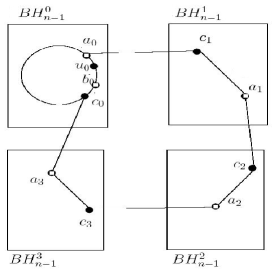
Figure 2: Illustration of 1.2.2

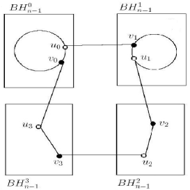
Figure 3: Illustration of 1.3.1.1

Subcase 1.3. There exist two distinct $i,k\in\{0,1,2,3\}$ such that $n-1\leq f_{i}\leq 2n-4$ and $n-1\leq f_{k}\leq 2n-4$. Without loss of generality, assume that $i=0$. Since $f\leq 2n-2$, it implies that $f_{0}=f_{k}=n-1$, $f_{c}=|F_{c}|=0$ and $f_{t}=0$ for any $t\in\{1,2,3\}-\{k\}$.

Subcase 1.3.1. $f_{v}^{0}\leq n-2$ and $f_{v}^{k}\leq n-2$.

By the inductive hypothesis, there exists a cycle $C_{0}$ (resp. $C_{k}$) in $BH_{n-1}^{0}$ (resp. $BH_{n-1}^{k}$) of length $2^{2(n-1)}-2f_{v}^{0}$ (resp. $2^{2(n-1)}-2f_{v}^{k}$).

Subcase 1.3.1.1. $k=1$ or $k=3$.

Since the discussion for the two situations are similar, we may assume $k=1$.

Note that $C_{0}$ has $2^{2(n-1)}-2f_{v}^{0}$ vertices, half is black and half is white, so there are $2^{2n-3}-f_{v}^{0}$ white vertices. We claim that there exist at least one white vertex in $C_{0}$ such that its extra neighbor in $C_{1}$. Since for each white vertex, say $u$, in $C_{0}$, there exists at most one other vertex $u^{\ast}$ in $C_{0}$, which has the same extra neighbors as $u$. So vertices in $C_{0}$ have at least $(2^{2n-3}-f_{v}^{0})/2$ extra neighbors in $C_{1}$. By $(2^{2n-3}-f_{v}^{0})/2>n-1=f_{1}$ because of $f_{v}^{0}\leq n-2$ and $n\geq 3$, there exists a white vertex $u_{0}\in V(C_{0})$ such that $u_{0}$ has an extra neighbor, say $v_{1}$, on $C_{1}$. See Figure 3.

Let $v_{0}$ be a neighbor of $u_{0}$ in $C_{0}$ and $u_{1}$ be a neighbor of $v_{1}$ in $C_{1}$. Let $u_{3}\in V(BH_{n-1}^{3})$ (resp. $v_{2}\in V(BH_{n-1}^{2})$) be an extra neighbor of $v_{0}$ (resp. $u_{1}$). Let $(v_{2},u_{3})\in E(BH_{n})$, where $v_{2}\in V(BH_{n-1}^{2})$ be a black vertex and $u_{3}\in V(BH_{n-1}^{3})$ be a white vertex. Since $f_{t}=0$ for $t\in\{2,3\}$, by Lemma 2.5, there exists a fault-free path $P_{t}$ of length $2^{2(n-1)}-1$ between $u_{t}$ and $v_{t}$ in $BH_{n-1}^{t}$. Let $P_{i}=C_{i}-(u_{i},v_{i})$ for $i=0,1$, then $\langle u_{0},P_{0},v_{0},u_{3},P_{3},v_{3},u_{2},P_{2},v_{2},u_{1},P_{1},v_{1},u_{0}\rangle$ is a fault-free cycle of length $2^{2n}-2f_{v}$ in $BH_{n}$.

Subcase 1.3.1.2. $k=2$.

Let $(u_{0},v_{0})\in C_{0}$ and assume $u_{0}$ is white. Choose an edge $(u_{2},v_{2})\in E(C_{2})$, assume $u_{2}$ is white. Let $v_{1}\in V(BH_{n-1}^{1})$ (resp. $u_{1}\in V(BH_{n-1}^{1})$, $v_{3}\in V(BH_{n-1}^{3})$ and $u_{3}\in V(BH_{n-1}^{3})$) be an extra neighbor of $u_{0}$ (resp. $v_{2}$, $u_{2}$ and $v_{0}$). Since $f_{t}=0$ for $t\in\{1,3\}$, by Lemma 2.5, there exists a fault-free path $P_{t}$ of length $2^{2(n-1)}-1$ between $u_{t}$ and $v_{t}$ in $BH_{n-1}^{t}$. Let $P_{i}=C_{i}-(u_{i},v_{i})$ for $i=0,2$, then $\langle u_{0},P_{0},v_{0},u_{3},P_{3},v_{3},u_{2},P_{2},v_{2},u_{1},P_{1},v_{1},u_{0}\rangle$ is a desired fault-free cycle of length $2^{2n}-2f_{v}$ in $BH_{n}$.

Subcase 1.3.2. $f_{v}^{0}=n-1$. (The discussion is similar for $f_{v}^{k}=n-1$.)

It implies $f_{v}^{k}=0$ and $f_{e}^{k}=n-1$. We regard one faulty vertex in $BH_{n-1}^{0}$ as fault-free, $f_{v}^{\prime}=f_{v}^{0}-1=n-2$. By the inductive hypothesis, there exists a cycle $C_{0}$ in $BH_{n-1}^{0}$ of length $2^{2(n-1)}-2f_{v}^{\prime}$, where $f_{v}^{\prime}=f_{v}^{0}-1=f_{v}-1$. Note that $C_{0}$ contains at most one faulty vertex. Without loss of generality, assume that $C_{0}$ contains one faulty vertex $u_{0}$ and $u_{0}$ is black. Let $a_{0}$ and $b_{0}$ be two vertices adjacent to $u_{0}$ in $C_{0}$. Let $c_{0}\in C_{0}$ be a neighbor of $b_{0}$. The desired cycle of $BH_{n}$ can be constructed by the similar discussions as Subcase 1.2.2, the details are omitted.

Case 2. There exists one $i\in\{0,1,2,3\}$ such that $f_{i}=2n-3$.

Without loss of generality, let $i=0$, i.e., $f_{0}=2n-3$. It implies that $f_{t}\leq f-f_{0}\leq 1$ for all $t\in\{1,2,3\}$. We consider the following two subcases.

Subcase 2.1. $f_{v}^{0}\leq n-2$.

Recall that $f_{e}^{0}=f_{0}-f_{v}^{0}\geq 2n-3-(n-2)=n-1\geq 2$ for $n\geq 3$. Choose any faulty edge, say $(u_{0},v_{0})\in E(BH_{n-1}^{0})$, regard $(u_{0},v_{0})$ as a fault-free edge temporarily, then $f_{0}-1\leq 2n-4$. By the inductive hypothesis, there exists a cycle $C_{0}$ of length $2^{2(n-1)}-2f_{v}^{0}$ in $BH_{n-1}^{0}$ such that $C_{0}$ contains at most one faulty edge $(u_{0},v_{0})$. Suppose $(u_{0},v_{0})\in E(C_{0})$ (otherwise choosing an edge in $E(C_{0})$ replace for $(u_{0},v_{0})$). Since there exists at most one faulty element outside $BH_{n-1}^{0}$, by Lemma 2.9(3), $(u_{0},v_{0})$ is contained in a fault-free cycle $C$, say $C=\langle v_{0},u_{0},v_{1},u_{1},v_{2},u_{2},v_{3},u_{3},v_{0}\rangle$, of length $8$ in $BH_{n}$ such that $E(C)\cap E(BH_{n-1}^{i})=\{(u_{i},v_{i})\}$ for each $i\in\{0,1,2,3\}$. Since $f_{t}\leq 1$ for all $t\in\{1,2,3\}$, note that $1\leq n-1$ and $1\leq 2n-3$ for $n\geq 3$, by Lemma 2.12 or Lemma 2.11, there exists a fault-free cycle $C_{t}$ of length $2^{2(n-1)}-2f_{v}^{t}$ passing through $(u_{t},v_{t})$. Let $P_{i}=C_{i}-(u_{i},v_{i})$ for $i\in\{0,1,2,3\}$, then $\langle u_{0},P_{0},v_{0},u_{3},P_{3},v_{3},u_{2},P_{2},v_{2},u_{1},P_{1},v_{1},u_{0}\rangle$ is a desired fault-free cycle of length $2^{2n}-2f_{v}$ in $BH_{n}$.

Subcase 2.2. $f_{v}^{0}=n-1$.

It implies $f_{v}^{j}=0$ and $f_{e}^{j}\leq 1$ for each $j\in\{1,2,3\}$. We regard one faulty vertex in $BH_{n-1}^{0}$ as fault-free temporarily. For the situation where $f_{0}-1\leq 2n-4$ and $f_{v}^{\prime}=f_{v}^{0}-1=f_{v}-1=n-2$, by the inductive hypothesis, there exists a cycle $C_{0}$ in $BH_{n-1}^{0}$ of length $2^{2(n-1)}-2f_{v}^{\prime}$, where $f_{v}^{\prime}=f_{v}^{0}-1$. Note that $C_{0}$ contains at most one faulty vertex.

If $C_{0}$ does not contain any faulty vertex, choose an edge, say $(u_{0},v_{0})\in E(C_{0})$ (assume $u_{0}$ is white, $v_{0}$ is black). By Lemma 2.9(3) and $f-f_{0}\leq 1$, $(u_{0},v_{0})$ is contained in a fault-free cycle $C$, say $C=\langle v_{0},u_{0},v_{1},u_{1},v_{2},u_{2},v_{3},\\ u_{3},v_{0}\rangle$, of length $8$ in $BH_{n}$ such that $E(C)\cap E(BH_{n-1}^{i})=\{(u_{i},v_{i})\}$ for each $i\in\{0,1,2,3\}$. By using the method similar to that of Subcase 1.2.2, we can find a desired cycle of length $2^{2n}-2f_{v}$ in $BH_{n}$. The details are omitted.

Now we assume that $C_{0}$ contains one faulty vertex $u_{0}$ and $u_{0}$ is black (if $u_{0}$ is white, the discussions are similar). Let $a_{0}$ and $b_{0}$ be two vertices adjacent to $u_{0}$ in $C_{0}$. Let $c_{0}\in C_{0}$ be a neighbor of $b_{0}$. Recall that each vertex has two extra neighbors and $f_{c}\leq 1$, we can choose the extra neighbors $c_{1}\in V(BH_{n-1}^{1})$ and $a_{3}\in V(BH_{n-1}^{3})$ of $a_{0}$ and $c_{0}$, respectively, such that both $(a_{0},c_{1})$ and $(c_{0},a_{3})$ are fault-free. The desired cycle of $BH_{n}$ can be constructed by the similar discussions as Subcase 1.2.2, the details are omitted.

Case 3. There exists one $i\in\{0,1,2,3\}$ such that $f_{i}=2n-2$.

Without loss of generality, let $i=0$, i.e. $f_{0}=f=2n-2$. It implies that $f_{j}=0$ for all $j\in\{1,2,3\}$ and $f_{c}=0$.

Since $f_{v}\geq 1$, we can choose a faulty vertex, say $w$ (assume $w$ is black, the discussion is similar for $w$ being white). Note that $f_{v}\leq n-1$, $f_{e}=f-f_{v}\geq 2n-2-(n-1)=n-1\geq 1$ for $n\geq 3$, let $(u_{0},v_{0})$ (assume $v_{0}$ is black) be a faulty edge. Image $w$ and $(u_{0},v_{0})$ as fault-free temporarily. Since $f_{0}-2\leq 2n-4$ and $f_{v}^{\prime}=f_{v}^{0}-1\leq n-1-1=n-2$, by the inductive hypothesis, there exists a cycle $C_{0}$ in $BH_{n-1}^{0}$ of length $2^{2(n-1)}-2f_{v}^{\prime}$, where $f_{v}^{\prime}=f_{v}^{0}-1=f_{v}-1$. Note that $C_{0}$ contains at most one faulty vertex $w$ and one faulty edge $(u_{0},v_{0})$. We consider the following four subcases.

Subcase 3.1. $w\notin C_{0}$ and $(u_{0},v_{0})\notin E(C_{0})$.

Choose any edge, say $(a_{0},b_{0})\in E(C_{0})$ (assume $a_{0}$ is white, $b_{0}$ is black). By Lemma 2.9(1) and $f_{c}=0$, $(a_{0},b_{0})$ is contained in a fault-free cycle $C$, say $C=\langle b_{0},a_{0},b_{1},a_{1},b_{2},a_{2},b_{3},a_{3},a_{0}\rangle$, of length $8$ in $BH_{n}$ such that $E(C)\cap E(BH_{n-1}^{i})=\{(a_{i},b_{i})\}$ for each $i\in\{0,1,2,3\}$. Since for any $i\in\{1,2\}$, $f_{i}=0$, by Lemma 2.5, there exists a fault-free path $P_{i}$ of length $2^{2(n-1)}-1$ between $a_{i}$ and $b_{i}$ in $BH_{n-1}^{i}$ for $i=1,2$. Since $f_{3}=0$, by Lemma 2.6, there exists a fault-free path $P_{3}$ of length $2^{2(n-1)}-3$ between $a_{3}$ and $b_{3}$ in $BH_{n-1}^{i}$. Let $P_{0}=C_{0}-(a_{0},b_{0})$. A desired fault-free cycle of $2^{2n}-2f_{v}$ in $BH_{n}$ can be constructed as $\langle a_{0},b_{1},P_{1},a_{1},b_{2},P_{2},a_{2},b_{3},P_{3},a_{3},b_{0},P_{0},a_{0}\rangle$.

Subcase 3.2. $w\notin C_{0}$ and $(u_{0},v_{0})\in E(C_{0})$.

By Lemma 2.9(1) and $f_{c}=0$, $(u_{0},v_{0})$ is contained in a cycle $C$, say $C=\langle v_{0},u_{0},v_{1},u_{1},v_{2},\\ u_{2},v_{3},u_{3},v_{0}\rangle$, of length $8$ in $BH_{n}$ such that $E(C)\cap E(BH_{n-1}^{i})=\{(u_{i},v_{i})\}$ and $(u_{i},v_{i+1})$ is fault-free for each $i\in\{0,1,2,3\}$. A desired cycle can be constructed by the similar discussion as Subcase 3.1, the details are omitted.

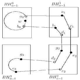
Figure 4: Illustration of 3.3;

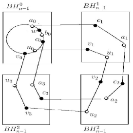
Figure 5: Illustration of 3.4.2

Subcase 3.3. $w\in C_{0}$ and $(u_{0},v_{0})\notin E(C_{0})$.

Let $a_{0}$ and $b_{0}$ be two vertices adjacent to $w$ in $C_{0}$. Since each vertex has two extra neighbors, let $a_{1}\in V(BH_{n-1}^{1})$, $b_{1}\in V(BH_{n-1}^{1})$ be an extra neighbor of $a_{0}$ and $b_{0}$, respectively, such that $a_{1}\neq b_{1}$. Choose two distinct white vertices, say $c_{i}$, $d_{i}$, respectively, in $BH_{n-1}^{i}$ for $i=1,2$. Let one of the extra neighbors of $c_{i}$, $d_{i}$ be $e_{i+1}$, $g_{i+1}$ in $BH_{n-1}^{i+1}$, respectively, for $i=1,2$. See Figure 5. By Lemma 2.8, there exist two vertex-disjoint paths $P_{1}[a_{1},c_{1}]$ and $R_{1}[b_{1},d_{1}]$ (resp. $P_{2}[c_{2},e_{2}]$ and $R_{2}[d_{2},g_{2}]$ ) in $BH_{n-1}^{1}$ (resp. $BH_{n-1}^{2}$) such that $V(P_{1}[a_{1},c_{1}])\cup V(R_{1}[b_{1},d_{1}])=V(BH_{n-1}^{1})$ (resp. $V(P_{2}[c_{2},e_{2}])\cup V(R_{2}[d_{2},g_{2}])=V(BH_{n-1}^{2})$). By Lemma 2.7, there exists a path $P_{3}$ in $V(BH_{n-1}^{3})$ of length $2^{2(n-1)}-2$ between $e_{3}$ and $g_{3}$. Since $f_{c}=0$, the crossing edges $(c_{1},e_{2})$, $(d_{1},g_{2})$, $(c_{2},e_{3})$, $(d_{2},g_{3})$ are fault-free. Let $P_{0}=C_{0}-\{w\}$. Thus, a fault-free cycle of length $2^{2n}-2f_{v}^{0}=2^{2n}-2f_{v}$ in $BH_{n}$ is $\langle a_{0},a_{1},P_{1}[a_{1},c_{1}],c_{1},e_{2},P_{2}[e_{2},c_{2}],c_{2},e_{3},P_{3},g_{3},d_{2},R_{2}[d_{2},g_{2}],g_{2},d_{1},R_{1}[d_{1},b_{1}],\\ b_{1},b_{0},P_{0},a_{0}\rangle$.

Subcase 3.4. $w\in C_{0}$ and $(u_{0},v_{0})\in E(C_{0})$.

Let $a_{0}$ and $b_{0}$ be two vertices adjacent to $w$ in $C_{0}$. If $v_{0}=w$, then $u_{0}=a_{0}$ or $u_{0}=b_{0}$. Without loss of generality, assume that $u_{0}=b_{0}$. The discussion is the same as that in Subcase 3.3.

Now we assume $v_{0}\neq w$ in the following. Notice that $u_{0}$ may equal to $a_{0}$ or $b_{0}$.

Subcase 3.4.1. $u_{0}=b_{0}$ (If $u_{0}=a_{0}$, the discussion is similar).

Assume that $C_{0}=\langle a_{0},w,u_{0},v_{0},P_{0}[v_{0},a_{0}],a_{0}\rangle$. For $i\in\{1,2,3\}$, let $u_{i}\in V(BH_{n-1}^{i})$ be a white vertex such that $(u_{3},v_{0})\in E(BH_{n})$. For $j\in\{1,2,3\}$, let $v_{j}\in V(BH_{n-1}^{j})$ be a black vertex such that $(a_{0},v_{1}),(u_{1},v_{2}),(u_{2},\\ v_{3})\in E(BH_{n})$. Since $f_{i}=0$ for $i\in\{1,2,3\}$, by Lemma 2.5, there exists a $u_{i}-v_{i}$ path $P_{i}$ of length $2^{2(n-1)}-1$ in $BH_{n-1}^{i}$. Thus, $\langle a_{0},v_{1},P_{1},u_{1},v_{2},P_{2},u_{2},\\ v_{3},P_{3},u_{3},v_{0},P_{0}[v_{0},a_{0}],a_{0}\rangle$ is a desired fault-free cycle of length $2^{2n}-2f_{v}$ in $BH_{n}$.

Subcase 3.4.2. $u_{0}\neq\{a_{0},b_{0}\}$.

Let $c_{1}\in V(BH_{n-1}^{1})$ (resp. $u_{3}\in V(BH_{n-1}^{3})$) be an extra neighbor of $a_{0}$ (resp. $v_{0}$). Let $c_{0}\in C_{0}$ be a neighbor of $b_{0}$ such that $c_{0}\neq v_{0}$ (otherwise let $c_{0}\in C_{0}$ be a neighbor of $a_{0}$, the discussion is similar). Thus $C_{0}$ is the type as $C_{0}=\langle a_{0},w,b_{0},c_{0},P_{0}[c_{0},u_{0}],u_{0},v_{0},P_{0}[v_{0},a_{0}],a_{0}\rangle$ (to see Figure 5). Since each vertex has two extra neighbors, let $v_{1}\in V(BH_{n-1}^{1})$ (resp. $a_{3}\in V(BH_{n-1}^{3})$) be an extra neighbor of $u_{0}$ (resp. $c_{0}$) such that $v_{1}\neq c_{1}$ (resp. $a_{3}\neq u_{3}$). For $i\in\{1,2\}$, let $u_{i},a_{i}\in V(BH_{n-1}^{i})$ be two distinct white vertices. For $j\in\{2,3\}$, let $v_{j},c_{j}\in V(BH_{n-1}^{j})$ be two distinct black vertices such that $(u_{j-1},v_{j})\in E(BH_{n})$ and $(a_{j-1},c_{j})\in E(BH_{n})$. Since $f_{i}=0$ for $i\in\{1,2,3\}$, by Lemma 2.8, there exist two vertex-disjoint paths $P_{i}[v_{i},u_{i}]$ and $R_{i}[c_{i},a_{i}]$ in $BH_{n-1}^{i}$ such that $V(P_{i}[v_{i},u_{i}])\cup V(R_{i}[c_{i},a_{i}])=V(BH_{n-1}^{i})$. Thus, a fault-free cycle of length $2^{2n}-2f_{v}$ in $BH_{n}$ is $\langle a_{0},c_{1},R_{1}[c_{1},a_{1}],a_{1},c_{2},R_{2}[c_{2},a_{2}],a_{2},c_{3},R_{3}[c_{3},a_{3}],a_{3},c_{0},P_{0}[c_{0},u_{0}],\\ u_{0},v_{1},P_{1}[v_{1},u_{1}],u_{1},v_{2},P_{2}[v_{2},u_{2}],u_{2},v_{3},P_{3}[v_{3},u_{3}],u_{3},v_{0},P_{0}[v_{0},a_{0}],a_{0}\rangle$.

By the above cases, the proof is complete.

4 Conclusion

In this paper, we obtained that $BH_{n}$ with $|F_{v}|+|F_{e}|\leq 2n-2$ and $|F_{v}|\leq n-1$ has a fault-free cycle of length $2^{2n}-2|F_{v}|$. If $|F_{v}|=0$, $|F_{e}|\leq 2n-2$, a fault-free cycle of length $2^{2n}-2|F_{v}|=2^{2n}$ is a Hamiltonian cycle. Since $BH_{n}$ is a bipartite graph with two partite sets of equal size, the cycle is the longest in the worst-case. Furthermore, since the edge connectivity of $BH_{n}$ is $2n$, the $BH_{n}$ cannot tolerate $2n-1$ faulty edges. Hence, our result is optimal in terms of faulty edges.

References

- [1] B. Alspach, D. Hare, Edge-pancyclic block-intersection graphs, Discrete Math. 97 (1991) 17–24.
- [2] J.A. Bondy, Pancyclic graphs, J. Combin. Theory 11 (1971) 80–84.
- [3] D. Cheng, R.-X. Hao, Various cycles embedding in faulty balanced hypercubes, Inform. Sci. 297 (2015) 140–153.
- [4] D. Cheng, R.-X. Hao, Y.-Q. Feng, Vertex-fault-tolerant cycles embedding in balanced hypercubes, Inform. Sci. 288 (2014) 449–461.
- [5] D. Cheng, R.-X. Hao, Y.-Q. Feng, Two node-disjoint paths in balanced hypercubes, Appl. Math. Comput. 242 (2014) 127–142.
- [6] Z.-Z. Du, J.-M. Xu, A note on cycle embedding in hypercubes with faulty vertices, Inform. Proces. Lett. 111 (2011) 557–560.
- [7] J.-S. Fu, Longest fault-free paths in hypercubes with vertex faults, Inform. Sci. 176 (2006) 759–771.
- [8] R.-X. Hao, R. Zhang, Y.-Q. Feng, J.-X. Zhou, Hamiltonian cycle embedding for fault tolerance in balanced hypercubes, Appl. Math. Comput. 244 (2014) 447–456.
- [9] S.-Y. Hsieh, Fault-tolerant cycle embedding in the hypercube with more both faulty vertices and faulty edges, Parall. Comput. 32 (2006) 84–91.
- [10] K. Huang, J. Wu, Balanced hypercubes, in: Proc. of the 1992, Int. Conf. Parallel Process. 3 (1992) 153–159.
- [11] K. Huang, J. Wu, Fault-tolerant resource placement in balanced hypercubes, Inform. Sci. 99 (1997) 159–172.
- [12] K. Huang, J. Wu, Area efficient layout of balanced hypercubes, Int. J. High Speed Electron. Syst. 6 (1995) 631–646.
- [13] H. Lü, X. Li, H. Zhang, Matching preclusion for balanced hypercubes, Theoret. Comput. Sci. 465 (2012) 10–20.
- [14] H. Lü, H. Zhang, Hyper-Hamiltonian laceability of balanced hypercubes, J. Supercomput. 68 (1) (2014) 302–314.
- [15] C.-H. Tsai, Fault-tolerant cycles embedded in hypercubes with mixed link and node failures, Appl. Math. Lett. 21 (2008) 855–860.
- [16] J. Wu, K. Huang, The balanced hypercubes: a cube-based system for fault-tolerant applications, IEEE Trans. Comput. 46 (4) (1997) 484–490.
- [17] J.-M. Xu, M. Ma, Survey on path and cycle embedding in some networks, Front. Math. China 4 (2009) 217–252.
- [18] M. Xu, X.-D. Hu, J.-M. Xu, Edge-pancyclicity and Hamiltonian laceability of the balanced hypercubes, Appl. Math. Comput. 189 (2007) 1393–1401.
- [19] M.-C. Yang, Bipanconnectivity of balanced hypercubes, Comput. Math. Appl. 60 (2010) 1859–1867.
- [20] M.-C. Yang, Super connectivity of balanced hypercubes, Appl. Math. Comput. 219 (2012) 970–975.
- [21] M.-C. Yang, Conditional diagnosability of balanced hypercubes under the PMC model, Inform. Sci. 222 (2013) 754–760.
- [22] M.-C. Yang, J.J.M. Tan, L.H. Hsu, Hamiltonian circuit and linear array embeddings in faulty -ary -cubes, J. Parall. Distrib. Comput. 67 (4) (2007) 362–368.
- [23] M.-C. Yang, M.-H. Yang, Reliability analysis of balanced hypercubes, IEEE COMCOMAP, (2012) 376–379.
- [24] W.-H. Yang, H.Z. Li, W.H. He, Edge-fault-tolerant bipancyclicity of Cayley graphs generated by transposition-generating trees, Inter. J. Comput. Math. 92(2015) 1345–1352.
- [25] J.-X. Zhou, Z.-L. Wu, S.-C. Yang, K.-W. Yuan, Symmetric property and reliability of balanced hypercube, IEEE Trans. Comput. 64 (2015) 876–881.
- [26] Q. Zhou, D. Chen, H. Lü, Fault-tolerant Hamiltonian laceability of balanced hypercubes, Inform. Sci. 300 (2015) 20–27.