Highly Efficient Computation of Generalized Inverse of a Matrix

V.Y. Pan ^a,c,, F. Soleymani ^b,, L. Zhao ^c,

^a Department of Mathematics and Computer Science, Lehman College of CUNY, Bronx, NY 10468, USA

^b Instituto Universitario de Matemática Multidisciplinar, Universitat Politècnica de València, 46022 València, Spain

^c Departments of Mathematics and Computer Science, The Graduate Center of CUNY, New York, NY 10036 USA

Abstract. We propose a hyperpower iteration for numerical computation of the outer generalized inverse of a matrix which achieves the 18th order of convergence by using only seven matrix multiplication per iteration loop. This is the record high efficiency for that computational task. The algorithm has a relatively mild numerical instability, and we stabilize it at the price of adding one extra matrix multiplication per iteration loop. This imlplies an efficiency index that significantly exceeds the known record for numerically stable iterations for this task. Our numerical tests cover a variety of examples such as Drazin case, rectangular case, and preconditioning of linear systems. The test results are in good accordance with our formal study and indicate that our algorithms can be of interest for the user.

2010 MSC: 15A09; 65F30; 15A23.

Keywords: Generalized inverses; hyperpower method; Moore-Penrose inverse; convergence analysis; Drazin inverse.

1. Our Subject, Motivation, Related Works, and Our Progress

1.1. Generalized inverses: some applications

It has been stated already by Forsythe et al. [12, p. 31] that in the great majority of practical computational problems, it is unnecessary and inadvisable to actually compute the inverse of a nonsingular matrix. This general rule still remains essentially true for modern matrix computations (see, e.g., [42, pages 39 and 180]). In contrast the computation or approximation of generalized inverses is required in some important matrix computations (cf., e.g., [24]). For example, generalized inverses are used for preconditioning large scale linear systems of equations [3, 8] and [5, pp. 171-208] and for updating the regression estimates based on the addition or deletion of the data in linear regression analysis [2, pp. 253-294]. Furthermore the computation of the so-called zero initial state system inverses for linear time-invariant state-space systems is essentially equivalent to determining generalized inverses of the matrices of the associated transfer functions.

There exists a generalized inverse of an arbitrary matrix, and it turns into a unique inverse when the matrix is nonsingular, but we must compute generalized inverses in order to deal with rectangular and rank deficient matrices [35, 40]. Some generalized inverses can be defined in any mathematical structure that involves associative multiplication, i.e., in a semigroup [47, chapter 1].

A system $Ax=b$ of linear equations has a solution if and only if the vector $A^{{\dagger}}b$ is a solution, and if so, then all solutions are given by the following expression:

(1.1) $$x=A^{{\dagger}}b+[I-A^{{\dagger}}A]w,$$

where we can choose an arbitrary vector $w$ and any generalized inverse $A^{{\dagger}}$.

1.2. Outer generalized inverse

Hereafter $\mathbb{C}^{m\times n}$ denotes the set of all complex $m\times n$ matrices, $\mathbb{C}_{r}^{m\times n}$ denotes the set of all complex $m\times n$ matrices of rank $r$, $I_{m}$ denotes the $m\times m$ identity matrix, and we drop the subscript if the dimension $m$ is not important or is clear from context. Furthermore $A^{*}$, $R(A)$, and $N(A)$ denote the conjugate (Hermitian) transpose, the Range, and the Null Space of a matrix $A$ $\in$ $\mathbb{C}^{m\times n}$, respectively.

For $A$ $\in$ $\mathbb{C}^{m\times n}$, outer generalized inverses or $\{2\}$-inverses are defined [2] by

(1.2) $$A\{2\}=\{X\in\mathbb{C}^{n\times m}:XAX=X\}.$$

For two fixed subspaces $S\in\mathbb{C}^{n}$ and $T\in\mathbb{C}^{m}$, define the generalized inverse $A_{T,S}^{(2)}\in A\{2\}$ of a complex matrix $A\in\mathbb{C}^{m\times n}$ as the matrix $X\in\mathbb{C}^{n\times m}$ such that $R(X)=T$ and $N(X)=S$.

Lemma 1.1.

Let a matrix $A\in\mathbb{C}^{m\times n}$ have rank $r$ and let $T$ and $S$ be subspaces of $\mathbb{C}^{n}$ and $\mathbb{C}^{m}$, respectively, with $dimT=dimS^{\perp}=t\leq r$. Then $A$ has a {2}$\textendash$inverse $X$ such that $R(X)=T$ and $N(X)=S$ if and only if

(1.3) $$AT\bigoplus S=\mathbb{C}^{m},$$

in which case $X$ is unique and is denoted by $A_{T,S}^{(2)}$ (see, e.g., [48]).

The traditional generalized inverses, e.g., the pseudo-inverse $A^{\dagger}$ (a.k.a. Moore-Penrose inverse), the weighted Moore-Penrose inverses $A_{MN}^{\dagger}$ (where $M$ and $N$ are two square Hermitian positive definite matrices), the Drazin-inverse $A^{D}$, the group inverse $A^{\#}$, the Bott-Duffin inverse $A_{L}^{-1}$ [33], the generalized Bott-Duffin inverse $A_{L}^{{\dagger}}$, and so on, each of special interest in matrix theory, are special cases of the generalized outer inverse $X=A_{T,S}^{(2)}$.

1.3. The known iterative algorithms for generalized inverses

A number of direct and iterative methods has been proposed and implemented for the computation of generalized inverses (e.g., see [26, 32]). Here we consider iterative methods. They approximate generalized inverse preconditioners, can be implemented efficiently in parallel architecture, converge particularly fast in some special cases (see, e.g., [22]), and compute various generalized inverses by using the same procedure for different input matrices, while direct methods usually require much more computer time and space in order to achieve such results.

Perhaps the most general and well-known scheme in this category is the following hyperpower iterative family of matrix methods [9, 39, 43],

(1.4) $$X_{k+1}=X_{k}(I+R_{k}+\cdots+R_{k}^{p-1})=X_{k}\sum\limits_{i=0}^{p-1}R_{k}^{i},\ \ \ R_{k}=I-AX_{k},\qquad k\geq 0.$$

Straightforward implementation of the iteration (1.4) of order $p$ involves $p$ matrix-matrix products. For $p=2$ it turns into the Newton-Schulz-Hotelling matrix iteration (SM), originated in [17, 30]:

(1.5) $$X_{k+1}=X_{k}(2I-AX_{k}),$$

and for $p=3$ into the cubically convergent method of Chebyshev-Sen-Prabhu (CM) [31]:

(1.6) $$X_{k+1}=X_{k}(3I-AX_{k}(3I-AX_{k})).$$

The paper [36] proposed the following seventh-order factorization (FM) for computing outer generalized inverse with prescribed range and null space assuming an appropriate initial matrix $X_{0}$ (see Section 4 for its choices):

(1.7) $$\left\{\begin{array}[]{l}\psi_{k}=I-AX_{k},\\ \zeta_{k}=I+\psi_{k}+\psi_{k}^{2},\\ \upsilon_{k}=\psi_{k}+\psi_{k}^{4},\\ X_{k+1}=X_{k}(I+\upsilon_{k}\zeta_{k}).\end{array}\right.$$

Chen and Tan [6] proposed computing $A_{T,S}^{(2)}$ by iterations based on splitting matrices.

For further background of iterative methods for computing generalized inverses, one may consult [18, pp. 82-84], [23, chapter 1], [24], [2], [5], [50]. Ben-Israel [1], Pan [25] and Sticrel [43] have presented general introductions into iterative methods for computing $A_{T,S}^{(2)}$. Recently such methods have been studied extensively together with their applications (see, e.g., [7, 21, 28]).

1.4. Our results

Our main results are two new algorithms in the form (1.4) for the generalized matrix inverse. They involve only 7 and 8 matrix-by-matrix products, respectively, and both of them achieve the convergence rate of 18. The efficiency index of the first algorithm (involving seven products) is record high, but the algorithm is numerically unstable, although mildly. Our second algorithm, using one extra matrix-by-matrix multiplication, is numerically stable. Its efficiency index is substantially higher than the previous record among numerically stable iterations for the same task. Our numerical tests showed that our algorithms are quite competitive and in most cases superior to the known algorithms in terms of the CPU time involved. All this should make our study theoretically and practically interesting.

1.5. Organization of the paper

In Section 2 we present our new algorithm. Its convergence and error analysis are the subjects of Section 3. In Section 4 we comment on the choice of the choice of an initial approximate inverse. In Section 5 we discuss its computational efficiency, while Section 6 is devoted to the analysis of its numerical stability. In Section 7 we present our second, numerically stable algorithm. Numerical tests, including the Drazin case, rectangular case, and preconditioning of large matrices, are covered in Section 8. We measure the performance by the number of iteration loops, the mean CPU time, and the error bounds. In our tests we compare performance of our algorithm and the known methods and show our improvement in terms of both computational time and accuracy. In Section 9 we present our brief concluding remarks and point out some further research directions.

2. Our First Fast Algorithm

It is well known that algorithm (1.5) has polylogarithmic complexity and is numerically stable and even self-correcting if the matrix $A$ is nonsingular, but otherwise is mildly unstable [34], [27]. Moreover it converges quite slowly in the beginning. Namely, its initial convergence is linear, and many iteration loops are generally required in order to arrive at the final quadratic convergence [14, pp. 259-287]. A natural remedy is provided by higher order matrix methods using fewer matrix-by-matrix multiplications, which are the cost dominant operations in hyperpower iterations (1.4).

Let $A\in\mathbb{C}^{m\times n}$, let $T$ and $S$ be subspaces of $\mathbb{C}^{n}$ and $\mathbb{C}^{m}$, respectively, with $dimT=dimS^{\perp}=t\leq r$, assume that $G\in\mathbb{C}^{n\times m}$ satisfies $R(G)\subseteq T$ and $N(G)\supseteq S$, and write $X_{0}=\alpha G$, for a nonzero real scalar $\alpha$ and a matrix $G$, both specified in Section 4. Now define a hyperpower iteration, for $p=18$ and any $k=0,1,2,\ldots$, by

(2.1) $$X_{k+1}=X_{k}(I+R_{k}+R_{k}^{2}+\cdots+R_{k}^{17}),\qquad R_{k}=I-AX_{k}.$$

The algorithm has the 18-th order of convergence and involves 18 matrix-by-matrix products per iteration loop, but we are going to use fewer products.

Based on factorization (2.1), we obtain (HM)

(2.2) $$X_{k+1}=X_{k}(R_{k}+I)\left(R_{k}^{2}-R_{k}+I\right)\left(R_{k}^{2}+R_{k}+I\right)\left(R_{k}^{6}-R_{k}^{3}+I\right)\left(R_{k}^{6}+R_{k}^{3}+I\right),$$

and consequently

(2.3) $$X_{k+1}=X_{k}(I+R_{k})\left(I+R_{k}^{2}+R_{k}^{4}+R_{k}^{6}+R_{k}^{8}+R_{k}^{10}+R_{k}^{12}+R_{k}^{14}+R_{k}^{16}\right).$$

Iterations (2.2) and (2.3) are clearly superior to the original scheme (2.1), but we will simplify them further.

Consider the following iterations,

(2.4) $$\begin{split}I+R_{k}^{2}+R_{k}^{4}+R_{k}^{6}+R_{k}^{8}+R_{k}^{10}+R_{k}^{12}+R_{k}^{14}+R_{k}^{16}=&(I+a_{1}R_{k}^{2}+a_{2}R_{k}^{4}+a_{3}R_{k}^{6}+R_{k}^{8})\\ &\times(I+b_{1}R_{k}^{2}+b_{2}R_{k}^{4}+b_{3}R_{k}^{6}+R_{k}^{8})+(\mu R_{k}^{2}+\psi R_{k}^{4})\end{split}$$

where we write $a_{3}=b_{3}$ and select seven nonzero real parameters $a_{1},a_{2},a_{3},b_{1},b_{2},b_{3},\mu,\psi$ from the following system of seven nonlinear equations:

(2.5) $$\left\{\begin{array}[]{l}\mu+a_{1}+b_{1}=1,\\[2.84526pt] a_{2}+\psi+a_{1}b_{1}+b_{2}=1,\\[2.84526pt] 2a_{3}+a_{2}b_{1}+a_{1}b_{2}=1,\\[2.84526pt] 2+a_{1}a_{3}+a_{3}b_{1}+a_{2}b_{2}=1,\\[2.84526pt] a_{1}+a_{2}a_{3}+b_{1}+a_{3}b_{2}=1,\\[2.84526pt] a_{2}+a_{3}^{2}+b_{2}=1,\\[2.84526pt] 2a_{3}=1.\end{array}\right.$$

We obtain

(2.6) $$a_{1}=\frac{5}{496}\left(31+\sqrt{93}\right),\quad a_{2}=\frac{1}{8}\left(3+\sqrt{93}\right),\quad a_{3}=\frac{1}{2},$$

(2.7) $$b_{1}=\frac{-5}{496}\left(\sqrt{93}-31\right),\quad b_{2}=\frac{1}{8}\left(3-\sqrt{93}\right),\quad\mu=\frac{3}{8},\quad\psi=\frac{321}{1984}.$$

Factorization (2.3) enables us to reduce the number of matrix-by-matrix multiplications to eight, but we are going to simplify this procedure further. We apply a similar strategy and deduce the following factorization:

(2.8) $$\begin{split}1+a_{1}R_{k}^{2}+a_{2}R_{k}^{4}+a_{3}R_{k}^{6}+R_{k}^{8}=&(1+c_{1}R_{k}^{2}+R_{k}^{4})(1+c_{2}R_{k}^{2}+R_{k}^{4})+(c_{3}R_{k}^{2}).\end{split}$$

By solving the nonlinear system of algebraic equations

(2.9) $$\left\{\begin{array}[]{l}c_{1}+c_{2}+c_{3}=a_{1},\\[2.84526pt] 2+c_{1}c_{2}=a_{2},\\[2.84526pt] c_{1}+c_{2}=a_{3},\end{array}\right.$$

we obtain

(2.10) $$c_{1}=\frac{1}{4}\left(\sqrt{27-2\sqrt{93}}+1\right),\quad c_{2}=\frac{1}{4}\left(1-\sqrt{27-2\sqrt{93}}\right),\quad c_{3}=\frac{1}{496}\left(5\sqrt{93}-93\right).$$

Furthermore write

(2.11) $$\begin{split}1+b_{1}R_{k}^{2}+b_{2}R_{k}^{4}+a_{3}R_{k}^{6}+R_{k}^{8}=&(1+c_{1}R_{k}^{2}+R_{k}^{4})(1+c_{2}R_{k}^{2}+R_{k}^{4})+(d_{1}R_{k}^{2}+d_{2}R_{k}^{4})\end{split}$$

and by solving the nonlinear system of equations

(2.12) $$\left\{\begin{array}[]{l}d_{1}+\frac{1}{2}=b_{1},\\[2.84526pt] \frac{1}{8}\left(8d_{2}+\sqrt{93}+3\right)=b_{2},\end{array}\right.$$

deduce that

(2.13) $$d_{1}=\frac{1}{496}\left(-93-5\sqrt{93}\right),\quad d_{2}=-\frac{\sqrt{93}}{4}.$$

Summarizing, we arrive at the following iterative method (PM) for computing generalized inverse:

(2.14) $$\left\{\begin{array}[]{l}R_{k}=I-AX_{k},\quad R_{k}^{2}=R_{k}R_{k},\quad R_{k}^{4}=R_{k}^{2}R_{k}^{2},\\[2.84526pt] M_{k}=(I+c_{1}R_{k}^{2}+R_{k}^{4})(I+c_{2}R_{k}^{2}+R_{k}^{4}),\\ T_{k}=M_{k}+c_{3}R_{k}^{2},\quad S_{k}=M_{k}+d_{1}R_{k}^{2}+d_{2}R_{k}^{4},\\ X_{k+1}=X_{k}((I+R_{k})((T_{k}S_{k})+\mu R_{k}^{2}+\psi R_{k}^{4})).\end{array}\right.$$

The iteration requires only seven matrix-by-matrix multiplications per loop, and as we show next, the algorithm has convergence rate eighteen.

3. Convergence and Error Analysis

In this section we present convergence and error analysis of our algorithm (2.14).

Theorem 3.1.

Assume that $A\in\mathbb{C}^{m\times n}_{r}$ and $G\in\mathbb{C}^{n\times m}_{s}$ is a matrix of rank $0<s\leq r$ such that $\mathrm{rank}({GA})=\mathrm{rank}({G})$. Then the sequence of matrix approximations $\{X_{k}\}_{k=0}^{k=\infty}$ defined by the matrix iteration (2.14) converges to $A_{R{(G)},N{(G)}}^{(2)}$ with the eighteenth order of convergence if the initial value $X_{0}=\alpha G$ satisfies

(3.1) $$\|F_{0}\|=\|AA_{T,S}^{(2)}-AX_{0}\|<1.$$

Here $\|\cdot\|$ denotes the spectral matrix norm.

Proof. Let us first define the residual matrix in the $k$th iterate of (2.14) by writing

(3.2) $$\mathcal{F}_{k}=AA_{T,S}^{(2)}-AX_{k}.$$

Equation (3.2) can be written as follows:

(3.3) $$\mathcal{F}_{k+1} =AA_{T,S}^{(2)}-AX_{k+1}$$

$$=AA_{T,S}^{(2)}-I+I-AX_{k+1}$$

$$=AA_{T,S}^{(2)}-I+I-A[X_{k}((I+R_{k})((T_{k}S_{k})+\mu R_{k}^{2}+\psi R_{k}^{4}))]$$

$$=AA_{T,S}^{(2)}-I+I-A\left[X_{k}(I+R_{k})\left(I+R_{k}^{2}+R_{k}^{4}+R_{k}^{6}+R_{k}^{8}+R_{k}^{10}+R_{k}^{12}+R_{k}^{14}+R_{k}^{16}\right)\right].$$

Equation (3.3) implies the following relationships:

(3.4) $$\mathcal{F}_{k+1} =AA_{T,S}^{(2)}-I+(I-AX_{k})^{18}$$

$$=AA_{T,S}^{(2)}-I+(I-AA_{T,S}^{(2)}+AA_{T,S}^{(2)}-AX_{k})^{18}$$

$$=AA_{T,S}^{(2)}-I+\left[(I-AA_{T,S}^{(2)})+\mathcal{F}_{k}\right]^{18}.$$

Therefore

(3.5) $$\mathcal{F}_{k+1} =AA_{T,S}^{(2)}-I+[I-AA_{T,S}^{(2)}+\mathcal{F}_{k}^{18}]$$

$$=\mathcal{F}_{k}^{18}.$$

Note that $(I-AA_{T,S}^{(2)})^{i}=0,\ i>1$, and that $\mathcal{E}_{k}=A_{R{(G)},N{(G)}}^{(2)}-X_{k}$ is the error matrix of the approximation of the outer generalized inverse $A_{T,S}^{(2)}$. Consequently

(3.6) $$A\mathcal{E}_{k+1} =AA_{R{(G)},N{(G)}}^{(2)}-AX_{k+1}=\mathcal{F}_{k+1}=\mathcal{F}_{k}^{18}.$$

By using equation (3.6) and some elementary algebraic transformations, we deduce that

(3.7) $$\|A\mathcal{E}_{k+1}\| \leq\|\mathcal{F}_{k}\|^{18}$$

$$=\|A\mathcal{E}_{k}\|^{18}$$

$$\leq\|A\|^{18}\|\mathcal{E}_{k}\|^{18}.$$

By applying inequality (3.7) and assuming that the integer $k$ is large enough, we estimate the rate of convergence as follows:

(3.8) $$\|\mathcal{E}_{k+1}\| =\|X_{k+1}-A_{R{(G)},N{(G)}}^{(2)}\|$$

$$=\left\|A_{R{(G)},N{(G)}}^{(2)}AX_{k+1}-A_{R{(G)},N{(G)}}^{(2)}AA_{R{(G)},N{(G)}}^{(2)}\right\|$$

$$=\left\|A_{R{(G)},N{(G)}}^{(2)}\left(AX_{k+1}-AA_{R{(G)},N{(G)}}^{(2)}\right)\right\|$$

$$\leq\|A_{R{(G)},N{(G)}}^{(2)}\|\,\|A\mathcal{E}_{k+1}\|$$

$$\leq\|A_{R{(G)},N{(G)}}^{(2)}\|\,\|A\|^{18}\,\|\mathcal{E}_{k}\|^{18}.$$

Therefore

(3.9) $$\{X_{k}\}_{k=0}^{k=\infty}\to A_{R{(G)},N{(G)}}^{(2)},$$

which shows that the convergence rate is eighteen. $\Box$

4. Stopping Criterion and the Choice of an Initial Approximate Inverse

According to [41], a reliable stopping criterion for a $p$th order matrix scheme can be expressed as follows:

(4.1) $$\frac{\|X_{k+1}-X_{k}\|_{*}}{p^{k}\alpha}<\epsilon,$$

where $\epsilon$ is the tolerance and $\alpha$ is the positive real number involved in the definition of an initial approximate inverse $X_{0}=\alpha G$.

We choose an initial approximation $X_{0}$ satisfying (3.1) in order to ensure convergence. It is sufficient to have this matrix in the form $X_{0}=\alpha G$ such that

(4.2) $$\left\|AA_{T,S}^{(2)}-AX_{0}\right\|<1.$$

By extending the idea of Pan and Schreiber [27], however, we can choose a more efficient initial value in the form $X_{0}=\alpha G$, where

(4.3) $$\alpha=\frac{2}{\sigma_{1}^{2}+\sigma_{r}^{2}},$$

and $\sigma_{1}\geq\sigma_{2}\geq\ldots\geq\sigma_{r}>0$ are the nonzero eigenvalues of $GA$.

Some initial approximations for matrices of various types are provided below. For a symmetric positive definite (SPD) matrix $A$, one can apply the Householder-John theorem [20] in order to obtain the initial value $X_{0}=P^{-1},$ where $P$ can be any matrix such that $P+P^{T}-A$ is SPD. A sub-optimal way of producing $X_{0}$ for the rectangular matrix $A$ had been given by $X_{0}=\frac{A^{*}}{\|A\|_{1}\|A\|_{\infty}}$. Also, for finding the Drazin inverse, one may choose the initial approximation $X_{0}=\frac{1}{\mathrm{Tr}({A^{l+1}})}A^{l}$ where $\mathrm{Tr}({\cdot})$ stands for the trace of a square matrix and $l$ for its index, $\mathrm{ind}({A})$, that is, the smallest nonnegative integer $l$ such that $rank(A^{l+1})$ $=rank(A^{l})$. The paper [13] proposes some further recipes for the construction of initial inverses specially in the case of square matrices.

5. Computational Efficiency

The customary concept of the efficiency index of iterative methods can be traced back to 1959 (see [11]). Traub in 1964 [45, Appendix C] used this index in his study of fixed-point iterations as follows,

(5.1) $$EI=p^{\frac{1}{c}}.$$

Here $c$ stands for the number of dominant cost operations per an iteration loop (in our case they are matrix-by-matrix multiplications), and $p$ denotes the local convergence rate.

Based on the work [37], we estimate that our method (2.14) converges with the errors within the machine precision in approximately

(5.2) $$s\approx 2log_{p}\kappa_{2}(A)$$

iteration loops where $\kappa_{2}(A)$ denotes the condition number of the matrix $A$ in spectral norm. Recall that our iteration (2.14) reaches eighteenth-order convergence by using only seven matrix-by-matrix multiplications. Here are the efficiency indices of various algorithms for generalized inverse:

(5.3) $$EI_{(\ref{schulz})}=2^{\frac{1}{2}}\approx 1.41421,\ EI_{(\ref{chebyshev})}=3^{\frac{1}{3}}\approx 1.44225,\ EI_{(\ref{SoleymaniN})}=7^{\frac{1}{5}}\approx 1.47577,$$

and

(5.4) $$EI_{(\ref{hyper18-2})}=18^{\frac{1}{9}}\approx 1.37872,\ EI_{(\ref{hyper18})}=18^{\frac{1}{18}}\approx 1.17419,\ EI_{(\ref{PM})}=18^{\frac{1}{7}}\approx\textbf{1.51121}.$$

The latter efficiency index is record high for iterative algorithms for generalized inverse.

6. Numerical Stability Estimates

In this section we study numerical stability of our iteration (2.14) in a neighborhood of the solution of the equation

(6.1) $$XAX-X=0.$$

We are going to estimate the rounding errors based on the first order error analysis [10]. We recall that iteration (1.4) is self-correcting for computing the inverse of a nonsingular matrix, but not so for computing generalized inverses [34], [27]. For the latter task our iteration (1.4) is numerically unstable, although the instability is rather mild, as we prove next. In Section 8 we complement our formal study by empirical results. In our next theorem we proceed under the same assumptions as in Theorem 3.1, allowing any initial approximation. In Theorem 6.2 we slightly improve the resulting estimate assuming the standard choice of an initial approximation in the form $X_{0}=\alpha A^{*}$ or more generally $X_{0}=A^{*}P(A^{*}A)$ for a constant $\alpha$ and a polynomial $P(x)$.

Theorem 6.1.

Consider the sequence $\{X_{k}\}_{k=0}^{k=\infty}$ generated by (2.14) under the same assumptions as in Theorem 3.1. Write

(6.2) $$\widetilde{X}_{k}=X_{k}+\Delta_{k}$$

for all $k$ assuming that $\Delta_{k}$ is a numerical perturbation of the $k$th exact iterate $X_{k}$ and has a sufficiently small norm, so that we can ignore quadratic and higher order terms in $\mathcal{O}(\Delta_{k}^{2})$.

Then

(6.3) $$\|\Delta_{k+1}\|\leq\mathcal{C}\|\Delta_{0}\|$$

where

(6.4) $$\mathcal{C}=18^{k+1}\prod_{j=0}^{k}[\max\{1,\|R_{j}\|^{17}\}(1+17\|A\|\|X_{j}\|)].$$

Proof. Write $\widetilde{R}_{k}=I-A\widetilde{X}_{k}$. Deduce that for each $j$, $j=1,...,17$,

(6.5) $$\|\widetilde{R}_{k}^{j}\| =\|(R_{k}-A\Delta_{k})^{j}\|$$

$$\leq\|R_{k}-A\Delta_{k}\|^{j}$$

$$\leq(\|R_{k}\|+\|A\Delta_{k}\|)^{j}$$

$$=C_{0}^{j},$$

where $C_{0}=\|R_{k}\|+\|A\Delta_{k}\|=\|R_{k}\|+\mathcal{O}(\|\Delta_{k}\|)$. Furthermore

(6.6) $$\|\widetilde{R}_{k}^{j}-R_{k}^{j}\| =\|(R_{k}-A\Delta_{k})^{j}-R_{k}^{j}\|$$

$$\leq(\|R_{k}\|+\|A\Delta_{k}\|)^{j}-\|R_{k}\|^{j}$$

$$=\|A\Delta_{k}\|(\sum_{i=0}^{j-1}{j\choose j-1-i}\|A\Delta_{k}\|^{i}\|R_{k}\|^{j-1-i})$$

$$=D_{j}\|A\Delta_{k}\|$$

for $D_{j}=\sum_{i=0}^{j-1}{j\choose j-1-i}\|A\Delta_{k}\|^{i}\|R_{k}\|^{j-1-i}=j\|R_{k}\|^{j-1}+\mathcal{O}(\|\Delta_{k}\|)$.

Then deduce that

(6.7) $$\Delta_{k+1} =\widetilde{X}_{k+1}-\widetilde{X}_{k}$$

$$=\widetilde{X}_{k}(I+\widetilde{R}_{k}+\widetilde{R}_{k}^{2}+\cdots+\widetilde{R}_{k}^{17})-X_{k}(I+R_{k}+R_{k}^{2}+\cdots+R_{k}^{17})$$

$$=(X_{k}+\Delta_{k})(I+(R_{k}-A\Delta_{k})+(R_{k}-A\Delta_{k})^{2}+\cdots+(R_{k}-A\Delta_{k})^{17})-X_{k}(I+R_{k}+R_{k}^{2}+\cdots+R_{k}^{17})$$

$$=\Delta_{k}\sum_{j=0}^{17}[\widetilde{R}_{k}^{j}]+X_{k}\sum_{i=0}^{17}[\widetilde{R}_{k}^{j}-R_{k}^{j}].$$

Therefore

(6.8) $$\|\Delta_{k+1}\| =\|\Delta_{k}\sum_{j=0}^{17}[\widetilde{R}_{k}^{j}]+X_{k}\sum_{i=0}^{17}[\widetilde{R}_{k}^{j}-R_{k}^{j}]\|$$

$$\leq\|\Delta_{k}\|\sum_{j=0}^{17}\|\widetilde{R}_{k}^{j}\|+\|X_{k}\|\sum_{i=0}^{17}\|\widetilde{R}_{k}^{j}-R_{k}^{j}\|$$

$$=\|\Delta_{k}\|\sum_{j=0}^{17}C_{0}^{j}+\|A\Delta_{k}\|\|X_{k}\|\sum_{i=0}^{17}D_{j}$$

$$\leq\|\Delta_{k}\|\sum_{j=0}^{17}[C_{0}^{j}+\|A\|\|X_{k}\|D_{j}]$$

$$<\|\Delta_{k}\|[18\max\{1,\|R_{k}\|^{17}\}(1+17\|A\|\|X_{k}\|)]+\mathcal{O}(\|\Delta_{k}\|).$$

This yields the claimed estimates (6.3) and (6.4) for numerical perturbation at iteration loop $k+1$. $\Box$

The following result a little refines the estimate of Theorem 6.1 under the standard choices of $X_{0}$.

Theorem 6.2.

Consider the same assumptions as in Theorem 3.1 and define singular value decompositions (SVDs)

(6.9) $$A=U\left[\begin{array}[]{cc}\Sigma&0\\ 0&0\end{array}\right]V^{T}$$

and

(6.10) $$A^{\dagger}=V\left[\begin{array}[]{cc}\Sigma^{\dagger}&0\\ 0&0\end{array}\right]U^{T}$$

for a matrix $A$ and its Moore-Penrose pseudo inverse $A^{\dagger}$. Moreover, let $X_{0}=\alpha A^{*}$ or more generally let $X_{0}=A^{*}P(A^{*}A)$ for a constant $\alpha$ and a polynomial $P(x)$. Then write

(6.11) $$X_{k}=A^{\dagger}+E_{k}=V\left[\begin{array}[]{cc}\Sigma^{\dagger}+E_{11}&E_{12}\\ E_{21}&E_{22}\end{array}\right]U^{T},$$

where $E_{k}$ is the error of approximation after $k$-th iteration loop. Then

(6.12) $$\|E_{k}\|\leq 18^{k}\|E_{0}\|+o(\|E_{0}\|).$$

Proof.

Throughout the proof drop all terms of second order in $E_{k}$. Let $R_{k}=I-AX_{k}$ and readily deduce that

(6.13) $$X_{k}R_{k}=V\left[\begin{array}[]{cc}-E_{11}&0\\ 0&E_{22}\end{array}\right]U^{T}$$

and that for $j\geq 2$ ,

(6.14) $$X_{k}R_{k}^{j}=V\left[\begin{array}[]{cc}0&0\\ 0&E_{22}\end{array}\right]U^{T}.$$

Thus

(6.15) $$X_{k+1} =X_{k}(I+R_{k}+\cdots+R_{k}^{17})$$

$$=V\left[\begin{array}[]{cc}\Sigma^{\dagger}&E_{12}\\ E_{21}&18E_{22}\end{array}\right]U^{T}$$

$$\leq A^{\dagger}+18\|\Delta_{k}\|$$

and therefore

(6.16) $$\Delta_{k}=X_{k}-A^{\dagger}\leq 18\|\Delta_{k-1}\|\leq\cdots\leq 18^{k}\|\Delta_{0}\|.$$

∎

Two remarks are in order.

1. The iteration is not self-correcting, and so proceeding beyond convergence may seriously increase error and cause divergence.

2. Our estimates above do not cover the influence of the rounding errors on the convergence [38]. The errors may imply slower convergence or even failure of the method, but this problem is alleviated in the iteration of the next section.

7. The Most Efficient Numerically Stable Iteration

In this section we modify iteration (1.4) by adding an extra matrix multiplication per iteration loop and then prove numerical stability of the modified iteration, which achieves the 18th order of convergence by performing eight matrix multiplications per iteration loop. Its efficiency index is $18^{1/8}>1.435$; this is substantially higher than the previous record high index among numerically stable iterations for this task, equal to $2^{1/3}<2.26$ (see (7.4) in [27]).

Theorem 7.1.

Consider the same assumption as in Theorem 6.2 and modify 2.14 as follows:

(7.1) $$\left\{\begin{array}[]{l}R_{k}=I-AX_{k},\quad R_{k}^{2}=R_{k}R_{k},\quad R_{k}^{4}=R_{k}^{2}R_{k}^{2},\\[2.84526pt] M_{k}=(I+c_{1}R_{k}^{2}+R_{k}^{4})(I+c_{2}R_{k}^{2}+R_{k}^{4}),\\ T_{k}=M_{k}+c_{3}R_{k}^{2},\quad S_{k}=M_{k}+d_{1}R_{k}^{2}+d_{2}R_{k}^{4},\\ X_{k+1/2}=X_{k}((I+R_{k})((T_{k}S_{k})+\mu R_{k}^{2}+\psi R_{k}^{4}))\\ X_{k+1}=X_{k+1/2}AX_{k+1/2}.\end{array}\right.$$

Observe that the modified iteration is numerically stable.

Proof.

Assume dealing with the modified procedure and readily verify that

(7.2) $$X_{k+1/2} =V\left[\begin{array}[]{cc}\Sigma^{\dagger}&E_{12}\\ E_{21}&18E_{22}\end{array}\right]U^{T}$$

and

(7.3) $$X_{k+1}=X_{k+1/2}AX_{k+1/2}=\left[\begin{array}[]{cc}\Sigma^{\dagger}&E_{12}\\ E_{21}&0.\end{array}\right].$$

Therefore

(7.4) $$\Delta_{k}=X_{k}-A^{\dagger}\leq\|\Delta_{k-1}\|\leq\cdots\leq\|\Delta_{0}\|.$$

∎

One can follow the semi-heuristic recipe of [27] by switching from iteration (1.4) to iteration (7.1) as soon as all significant singular values have been suppressed.

8. Numerical Experiments

In this section, we present the results of our numerical experiments for algorithm (2.14). We applied Mathematica 10.0 [46, pp. 203-224] and carried out our demonstrations with machine precision (except for the first test) on a computer with the following specifications: Windows 7 Ultimate, Service Pack 1, Intel(R) Core(TM) i5-2430M CPU 2.40GHz, and 8.00 GB of RAM.

For the sake of comparisons, we applied the methods SM, CM, FM, HM and PM, setting the maximum number of iteration loops to 100. We calculated running time by applying the command $\mathtt{AbsoluteTiming[]}$, which reported the elapsed computational time (in seconds).

We computed the order of convergence in our first experiment by using the following expression [37],

(8.1) $$\rho=\frac{\ln\left((\|X_{k+1}-X_{k}\|)(\|X_{k}-X_{k-1}\|)^{-1}\right)}{\ln\left((\|X_{k}-X_{k-1}\|)(\|X_{k-1}-X_{k-2}\|)\right)^{-1}}.$$

Here $\|\cdot\|$ denotes the infinity norm $\|\cdot\|_{\infty}$.

Table 1. The results of experiments for Example 8.1.

Methods		SM	CM	FM	PM
$\rho$		2.00	3.00	7.00	18.00
IT		17	11	7	5
$R_{k+1}$		$3.712\times 10^{-66}$	$1.833\times 10^{-59}$	$6.3\times 10^{-120}$	$7.474\times 10^{-107}$

Example 8.1.

In our first series of experiments, we compared various methods for finding the Drazin inverse of the following matrix,

(8.2) $$A=\left[\begin{array}[]{cccccccccccc}2&4/10&0&0&0&0&0&0&0&0&0&0\\ -2&4/10&0&0&0&0&0&0&0&0&0&0\\ -1&-1&1&-1&0&0&0&0&-1&0&0&0\\ -1&-1&-1&1&0&0&0&0&0&0&0&0\\ 0&0&0&0&1&1&-1&-1&0&0&-1&0\\ 0&0&0&0&1&1&-1&-1&0&0&0&0\\ 0&0&0&-1&-2&4/10&0&0&0&0&0&0\\ 0&0&0&0&2&4/10&0&0&0&0&0&0\\ 0&-1&0&0&0&0&0&0&1&-1&-1&-1\\ 0&0&0&0&0&0&0&0&-1&1&-1&-1\\ 0&0&0&0&0&0&0&0&0&0&4/10&-2\\ 0&0&0&0&0&0&0&0&0&0&4/10&2\end{array}\right],$$

where $l=\mathrm{ind}({A})=3$, and we used 150 fixed floating point digits. The results for this example are given in Table 1, where IT stands for the number of iteration loops and $R_{k+1}=\|X_{k+1}-X_{k}\|_{\infty}$ with the $R_{k+1}\leq\epsilon=10^{-50}$ and $X_{0}=\frac{1}{\mathrm{Tr}({A^{l+1}})}A^{l}$.

Example 8.2.

In this series of experiments, we compared computational time of various algorithms for computing the Moore-Penrose inverse of 10 rectangular ill-conditioned Hilbert matrices

(8.3) $$H_{m\times n}=\left[\frac{1}{i+j-1}\right]_{m\times n}.$$

We used stopping criterion (4.1) with the Frobenius norm and with the initial approximation $X_{0}=\frac{2}{\sigma_{1}^{2}+\sigma_{r}^{2}}H^{T}$. The results are displayed in Tables 2-4.

Matrix No.	SM	CM	HM	PM
$H_{100\times 90}$	0.049003	0.047003	0.048003	0.047003
$H_{200\times 190}$	0.229013	0.220013	0.224013	0.211012
$H_{300\times 290}$	0.435025	0.380022	0.414024	0.388023
$H_{400\times 390}$	0.976056	0.908052	0.920053	0.941054
$H_{500\times 490}$	1.647094	1.531088	1.652095	1.611092
$H_{600\times 590}$	2.595148	2.464141	2.628150	2.505143
$H_{700\times 690}$	3.842220	3.619207	3.956226	3.645208
$H_{800\times 790}$	5.509315	5.131293	5.563318	5.113292
$H_{900\times 890}$	7.238414	6.880394	7.943454	6.872393
$H_{1000\times 990}$	9.441540	9.019516	10.208584	9.012523

Table 2. The elapsed time for Example 8.2 by using $\epsilon=10^{-5}$.

Matrix No.	SM	CM	HM	PM
$H_{100\times 90}$	0.047003	0.038002	0.047003	0.045003
$H_{200\times 190}$	0.218012	0.194011	0.192011	0.190011
$H_{300\times 290}$	0.387022	0.349020	0.343020	0.337019
$H_{400\times 390}$	0.833048	0.740042	0.809046	0.794045
$H_{500\times 490}$	1.407080	1.373079	1.436082	1.318075
$H_{600\times 590}$	2.273130	2.162124	2.285131	2.067118
$H_{700\times 690}$	3.287188	3.166181	3.351192	3.057175
$H_{800\times 790}$	4.617264	4.405252	4.745271	4.269244
$H_{900\times 890}$	6.221356	5.952341	6.403366	5.784331
$H_{1000\times 990}$	8.124465	7.841449	8.524487	7.553432

Table 3. The elapsed time for Example 8.2 by using $\epsilon=10^{-6}$.

Matrix No.	SM	CM	HM	PM
$H_{100\times 90}$	0.055003	0.053003	0.048003	0.051003
$H_{200\times 190}$	0.231013	0.233013	0.216012	0.227013
$H_{300\times 290}$	0.463027	0.388022	0.412024	0.406023
$H_{400\times 390}$	0.975056	0.901052	0.933053	0.942054
$H_{500\times 490}$	1.629093	1.568090	1.643094	1.599092
$H_{600\times 590}$	2.651152	2.502143	2.701154	2.471141
$H_{700\times 690}$	3.801217	3.593205	3.992228	3.651209
$H_{800\times 790}$	5.508315	5.130293	5.639323	5.044289
$H_{900\times 890}$	7.192411	6.872393	7.779445	6.890394
$H_{1000\times 990}$	9.508544	9.211527	10.687611	9.177525

Table 4. The elapsed time for Example 8.2 by using $\epsilon=10^{-7}$.

We compared the efficiency of our iteration (2.14) and the known methods. Like the known methods, our iteration converged consistently, but run faster, in good accordance with the formal analysis. Overall the test results in Tables 1-4 confirm some advantages of our iteration in terms of the order of convergence and computational time in most of the tested cases.

Example 8.3.

Finally we compared the preconditioners obtained from our algorithm with the known preconditioners based on Incomplete LU factorizations [29] and applied to the solution of the sparse linear systems, $Ax=b$, of the dimension 841 by using GMRES. The matrix $A$ has been chosen from MatrixMarket [16] database as

(8.4) $$\mathtt{A=ExampleData[{"Matrix","YOUNG1C"}]},$$

with the right hand side vector $b=(1,1,...,1)^{T}$. The solution in this case is given by the vector $(-0.0177027-0.00693171I$, …, $-0.0228083-0.00589176I)^{T}$. Figure 1 shows the plot of the matrix $A$ (note that this matrix is not tridiagonal), while Figure 2 reveals the effectiveness of our scheme for preconditioning.

The left preconditioned system using $X_{5}$ of SM, $X_{3}$ of CM, and $X_{1}$ of PM, along with the well-known preconditioning techniques $\mathtt{ILU0}$, $\mathtt{ILUT}$ and $\mathtt{ILUTP}$ have been tested, while the initial vector has been chosen in all cases automatically, by the command $\mathtt{LinearSolve[]}$ in Mathematica 10. The results of time comparisons for various values of tolerance to the residual norms have been shown in Figure 2. In our tests, as could be expected, the computational time increased as tolerance decreased, but the preconditioner $X_{1}$ from the method PM mostly yielded the best feedbacks. For these tests, we used the following initial matrix from [44],

(8.5) $$X_{0}=diag(1/a_{11},1/a_{22},\cdots,1/a_{nn}),$$

where $a_{ii}$ denoted the $i$th diagonal entry of $A$.

After a few iteration loops, the computed preconditioner of the Schulz-type methods can be dense. Accordingly, we must choose a strategy for controlling the sparseness of the preconditioner. We can do this by setting the Mathematica command $\mathtt{Chop[X,10^{-5}]}$, at the end of each cycle for these matrices.

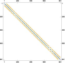
Figure 1. The plot of the matrix $A$ in Example 8.3.

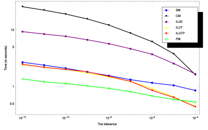
Figure 2. The results of comparisons in terms of the computational time.

9. Concluding comments

The calculation of generalized inverse is an inalienable part of some important matrix computations (see our Section 1.1).

In this paper, we propose a fast and numerically reliable iterative algorithm (2.14) for the outer generalized inverse $A^{(2)}_{T,S}$ of a matrix $A$. The algorithm has the eighteenth order of convergence and uses only seven matrix-by-matrix multiplications per iteration loop. This implies the record high computational efficiency index, $\approx 1.511.21$. As usual for the iterative algorithms of this class, our iteration is self-correcting for computing the inverse of a nonsingular matrix, but not for computing generalized inverses. For that task, the algorithm has mild numerical instability, but at the expense of performing an extra matrix multiplication per iteration loop, we obtain numerically stable algorithm, still having the eighteenth order of convergence. This greatly increases the previous record efficiency index, this time in the class of numerically stable iterations for generalized inverses. The results of our analysis and of our tests indicate that our algorithms are quite promising for practical use in computations with both double and multiple precision. We found out that for high order methods such as (2.14), it is usually sufficient to perform one full cycle iteration in order to produce an approximate inverse preconditioner.

Further increase of the convergence order and decrease of the number of matrix multiplications per iteration loop (both under the requirement of numerical stability and with allowing mild instability) are natural goals of our future research. We are going to extend it also to the acceleration of the known iterative algorithms for various other matrix equations (cf. [15], [4]).

References

- [1] A. Ben-Israel, An iterative method for computing the generalized inverse of an arbitrary matrix, Math. Comput. 19 (1965), 452-455.
- [2] A. Ben-Israel, T.N.E. Greville, Generalized Inverses, 2nd ed. Springer, New York, 2003.
- [3] M. Benzi, M. Tuma, Numerical experiments with two approximate inverse preconditioners, BIT 38, (1998), 234-241.
- [4] D.A. Bini, B. Iannazzo, B. Meini, Numerical Solution of Algebraic Riccati Equations, SIAM Publications, Philadelphia, PA, 2012.
- [5] S.L. Campbell, C.D. Meyer, Generalized Inverses of Linear Transformations, SIAM Publications, Philadelphia, PA, 2009.
- [6] Y. Chen, X. Tan, Computing generalized inverses of matrices by iterative methods based on splittings of matrices, Appl. Math. Comput. 163 (2005), 309-325.
- [7] G. Codevico, V.Y. Pan, M. V. Barel, Newton-like iteration based on a cubic polynomial for structured matrices, Numer. Algorithms, 36 (2004), 365-380.
- [8] E. Chow, Y. Saad, Approximate inverse preconditioners via sparse-sparse iterations, SIAM J. Sci. Comput., 19 (1998), 995-1023.
- [9] J.-J. Climent, N. Thome, Y. Wei, A geometrical approach on generalized inverses by Neumann-type series, Linear Algebra Appl. 332-334 (2001), 533-540.
- [10] J.J. Du Croz, N.J. Higham, Stability of methods for matrix inversion, IMA J. Numer. Anal. 12 (1992), 1-19.
- [11] H. Ehrmann, Konstruktion und Durchführung von Iterationsverfahren höherer Ordnung, Arch. Ration. Mech. Anal. 4 (1959), 65-88.
- [12] G.E. Forsythe, M.A. Malcolm, C.B. Moler, Computer Methods for Mathematical Computations, Englewood Cliffs, NJ: Prentice-Hall, 1977.
- [13] L. González, A. Suárez, Improving approximate inverses based on Frobenius norm minimization, Appl. Math. Comput., 219 (2013), 9363-9371.
- [14] N.J. Higham, Accuracy and Stability of Numerical Algorithms, Society for Industrial and Applied Mathematics, 2nd edition, 2002.
- [15] N. J. Higham, Functions of Matrices: Theory and Computations, SIAM, Philadelphia, 2008.
- [16] http://math.nist.gov/MatrixMarket/.
- [17] H. Hotelling, Some new methods in matrix calculation, Annals of Math. Stat., 14 (1943), 1-34.
- [18] E. Isaacson, H.B. Keller, Analysis of Numerical Methods, Wiley, New York, 1966.
- [19] T. Kailath, A. Vieira, M. Morf, Inverses of Toeplitz operators, innovations and orthogonal polynomials, SIAM Rev. 20 (1978), 106-119.
- [20] H.-B. Li, T.-Z. Huang, Y. Zhang, X.-P. Liu, T.-X. Gu, Chebyshev-type methods and preconditioning techniques, Appl. Math. Comput. 218 (2011), 260-270.
- [21] X. Liu, H. Huang, Higher-order covergent iterative method for computing the generalized inverse over Banach spaces, Abstr. Appl. Anal. 2013 (2013), 5 pages, Article ID 356105.
- [22] X. Liu, H. Jin, Y. Yu, Higher-order convergent iterative method for computing the generalized inverse and its application to Toeplitz matrices, Linear Algebra Appl., 439 (2013), 1635-1650.
- [23] M.Z. Nashed, Generalized Inverse and Applications, Academic Press, New York, 1976.
- [24] M.Z. Nashed, X. Chen, Convergence of Newton-like methods for singular operator equations using outer inverses, Numer. Math. 66 (1993), 235-257.
- [25] V.Y. Pan, Newton’s iteration for matrix inversion, advances and extensions, In: Matrix Methods: Theory, Algorithms and Applications. Singapore: World Scientific, 2010.
- [26] V.Y. Pan, M. Kunin, R. Rosholt, H. Kodal, Homotopic residual correction processes, Math. Comput., 75 (2006), 345-368.
- [27] V.Y. Pan, R. Schreiber, An improved Newton iteration for the generalized inverse of a matrix with applications, SIAM J. Sci. Stat. Comput., 12 (1991), 1109-1131.
- [28] M.D. Petković, M.S. Petković, Hyper-power methods for the computation of outer inverses, J. Comput. Appl. Math. 278 (2015), 110–118.
- [29] Y. Saad, Iterative Methods for Sparse Linear Systems, 2ed., SIAM, USA, 2003.
- [30] G. Schulz, Iterative Berechnung der Reziproken matrix, Z. Angrew. Math. Mech. 13 (1933), 57-59.
- [31] S.K. Sen, S.S. Prabhu, Optimal iterative schemes for computing Moore-Penrose matrix inverse, Int. J. Sys. Sci. 8 (1976), 748-753.
- [32] R. Schreiber, Computing generalized inverses and eigenvalues of symmetric matrices using systolic arrays, in: R. Glowinski, J.L. Lious (Eds.), Computing Methods in Applied Science and Engineering, North-Holland, Amsterdam, 1984.
- [33] X. Sheng, An iterative algorithm to compute the Bott-Duffin inverse and generalized Bott-Duffin inverse, Filomat, 26 (2012), 769-776.
- [34] T. Söderstörm, G.W. Stewart, On the numerical properties of an iterative method for comuting the Moore-Penrose generalized inverse, SIAM J. Numer. Anal. 11 (1974), 61-74.
- [35] F. Soleimani, P.S. Stanimirović, F. Soleymani, Some matrix iterations for computing generalized inverses and balancing chemical equations, Algorithms (Basel), 8 (2015), 982-998.
- [36] F. Soleymani, An efficient and stable Newton-type iterative method for computing generalized inverse , Numer. Algor. 69 (2015), 569-578.
- [37] F. Soleymani, On finding robust approximate inverses for large sparse matrices, Linear Multilinear Algebra 62 (2014), 1314-1334.
- [38] F. Soleymani, P.S. Stanimirović, A note on the stability of a th order iteration for finding generalized inverses, Appl. Math. Lett. 28 (2014) 77-81.
- [39] F. Soleymani, P.S. Stanimirović, F. Khaksar Haghani, On hyperpower family of iterations for computing outer inverses possessing high efficiencies, Linear Algebra Appl., 484 (2015), 477-495.
- [40] P.S. Stanimirović, S. Chountasis, D. Pappas, I. Stojanović, Removal of blur in images based on least squares solutions, Math. Meth. Appl. Sci. 36 (2013), 2280–2296.
- [41] P.S. Stanimirović, F. Soleymani, F. Khaksar Haghani, Computing outer inverses by scaled matrix iterations, J. Comput. Appl. Math., 296 (2016), 89-101.
- [42] G.W. Stewart, Matrix Algorithms, Vol I: Basic Decompositions, SIAM, Philadelphia, 1998.
- [43] E. Sticrel, On a class of high order methods for inverting matrices, ZAMM Z. Angew. Math. Mech. 67 (1987), 331-386.
- [44] P. Tarazaga, D. Cuellar, Preconditioners generated by minimizing norms, Comput. Math. Appl., 57 (2009), 1305-1312.
- [45] J.F. Traub, Iterative Methods for Solution of Equation, Prentice-Hall, Englewood Cliffs, NJ, 1964.
- [46] M. Trott, The Mathematica Guidebook for Numerics, Springer, New York, NY, USA, 2006.
- [47] G. Wang, Y. Wei, S. Qiao, Generalized Inverses: Theory and Computations, Science Press, Beijing/New York, 2004.
- [48] Y. Wei, H. Wu, The representation and approximation for the generalized inverse , Appl. Math. Comput. 135 (2003), 263–276.
- [49] J.H. Wilkinson, Error analysis of direct methods of matrix inversion, Assoc. Comput. Mach. 8 (1961), 281-330.
- [50] B. Zheng, R.B. Bapat, Generalized inverse and a rank equation, Appl. Math. Comput., 155 (2004), 407–415.