Cosmology from large scale galaxy clustering and galaxy-galaxy lensing with Dark Energy Survey Science Verification data
Abstract
We present cosmological constraints from the Dark Energy Survey (DES) using a combined analysis of angular clustering of red galaxies and their cross-correlation with weak gravitational lensing of background galaxies. We use a 139 square degree contiguous patch of DES data from the Science Verification (SV) period of observations. Using large scale measurements, we constrain the matter density of the Universe as and the clustering amplitude of the matter power spectrum as after marginalizing over seven nuisance parameters and three additional cosmological parameters. This translates into S for our fiducial lens redshift bin at 0.35 0.5, while S using two bins over the range 0.2 0.5. We study the robustness of the results under changes in the data vectors, modelling and systematics treatment, including photometric redshift and shear calibration uncertainties, and find consistency in the derived cosmological parameters. We show that our results are consistent with previous cosmological analyses from DES and other data sets and conclude with a joint analysis of DES angular clustering and galaxy-galaxy lensing with Planck CMB data, Baryon Accoustic Oscillations and Supernova type Ia measurements.
1 Introduction
Since the discovery of cosmic acceleration, the nature of dark energy has emerged as one of the most important open problems in cosmology. Wide-field, large-volume galaxy surveys are promising avenues to answer cosmological questions, since they provide multiple probes of cosmology, such as Baryon Acoustic Oscillations (BAO), large scale structure, weak lensing and cluster counts from a single dataset. Moreover, some of these probes can be combined for greater effect, since each is sensitive to their own combination of cosmological parameters and systematic effects. In this paper, we will focus on combining the large scale angular clustering of galaxies with measurements of the gravitational lensing produced by the large scale structure traced by the same galaxies, as observed in the Dark Energy Survey (DES). Measurements of the large scale clustering of galaxies are among the most mature probes of cosmology. The positions of galaxies are seeded by the distribution of dark matter on large scales and the manner in which the growth of structure proceeds from gravitational collapse is sensitive to the relative amounts of dark matter and energy in the Universe. There is a long history of using large-volume galaxy surveys for the purposes of constraining cosmology, including DES, Sloan Digital Sky Survey (SDSS) (York et al., 2000), Hyper Suprime-Cam (HSC) (Miyazaki et al.,, 2012), the Kilo-Degree Survey (KiDS) (de Jong et al., 2013, 2015; Kuijken et al., 2015), and the Canada France Hawaii Telescope Lensing Survey (CFHTLenS) (Heymans et al., 2012; Erben et al., 2013). Gravitational lensing, the deflection of light rays by massive structures, provides a complementary method of probing the matter distribution. Here we focus on galaxy-galaxy lensing (Tyson et al., 1984; Brainerd, Blandford & Smail, 1996), when both the lenses and sources are galaxies. This involves correlating the amount of distortion in the shapes of background galaxies with the positions of foreground galaxies. The amount of distortion is indicative of the strength of the gravitational potential of the lens and therefore tells us about the amount of matter contained in the lens plane. Weak gravitational lensing produces two effects, magnification of the source and shearing of its image, but this analysis is only concerned with the latter. These have been used to probe both cosmology (Mandelbaum et al., 2013; Cacciato et al., 2013; More et al., 2015) and the structure of dark matter halos and its connection to the galaxy distribution and baryon content of the Universe (Sheldon et al., 2004; Mandelbaum et al., 2006, 2008; Cacciato et al., 2009; Leauthaud et al., 2012; Gillis et al., 2013; Velander et al., 2014; Hudson et al., 2015; Sifón et al., 2015; Viola et al., 2015; van Uitert et al., 2016). Individual studies of large scale structure (Crocce et al., 2015), galaxy-galaxy lensing (Clampitt et al., 2016) and cosmic shear (Becker et al., 2015; The Dark Energy Survey Collaboration, 2015) using DES data as well as combined analyses focusing on smaller scales (Park et al., 2015) have been presented elsewhere. In this paper, we combine angular clustering and galaxy-galaxy lensing to jointly estimate the large-scale galaxy bias and matter clustering and constrain cosmological parameters. The plan of the paper is as follows. Section 2 outlines the theoretical framework for modelling the angular galaxy correlation function and galaxy-galaxy lensing. Section 3 describes the galaxy sample used and the measurements from DES data, as well as the covariance between the two probes. Our cosmology results are summarized in Section 4 including constraints on a five-parameter CDM (Cold Dark Matter) model and a six-parameter CDM model, where , the dark energy equation of state parameter is also allowed to vary. We discuss the robustness of our results and our tests for systematic errors in Section 5. Finally, we combine our analysis with other probes of cosmology and compare our results to previous results in the literature in Section 6. Our conclusions are presented in Section 7.
2 Theory
We are interested in describing the angular clustering of galaxies, , and the tangential shear produced by their host dark matter halos, , as a function of cosmology. The angular correlation function, , can be expressed in terms of the galaxy power spectrum as:
| (1) | |||||
| (2) |
where is the galaxy auto power spectrum, is the Bessel function of order 0, is the angular wavenumber, is the comoving radial co-ordinate, is the Hubble relation, is the speed of light, and is the number of galaxies as a function of radial distance from the observer, normalized such that . Note that Eq. 2 uses the Limber approximation (Limber, 1953; Kaiser, 1992), such that the radial distribution of galaxies, , is assumed to be slowly varying over our redshift slice. We have also ignored the contribution of redshift-space distortions to the angular clustering; this is expected to be small due to the width of the redshift intervals used; for the full expression, see Crocce et al. (2015). The tangential shear is given by:
| (3) |
where is the lens efficiency, is the scale factor and and are the selection functions of the lenses (foreground) and source (background) galaxies respectively. The foreground galaxies supply the gravitational potentials that lens the background galaxies. The tangential shear is a measurement of the amount of distortion introduced into the images of background galaxies from the gravitational potentials of foreground galaxies as a function of scale. We will discuss the impact of photometric redshift (photo-) errors on the lens and source distributions and propagate these to the measured cosmological constraints in Section 5. The combination of these two probes has been extensively discussed in the literature (Baldauf et al., 2010; Yoo & Seljak, 2012; Mandelbaum et al., 2013; Park et al., 2015) and provide another means by which we can mine the rich, well calibrated DES-SV dataset. Unlike Park et al. (2015), we restrict our modelling to sufficiently large scales such that we are not sensitive to how galaxies populate individual halos, i.e. Halo Occupation Distribution (HOD) modelling is unnecessary. On these scales, we are only concerned with correlations between galaxies that reside in different halos (the 2-halo term of the power spectrum), and we can relate the matter power spectrum, , to the galaxy power spectrum and galaxy-dark matter cross-power spectrum via the following relationships:
| (4) | |||
| (5) |
where is the linear bias that relates the clustering of galaxies to that of dark matter and is the cross-correlation coefficient that captures the stochasticity between the clustering of dark matter and the clustering of galaxies; see for example Seljak (2000); Guzik & Seljak (2001). The measurement of depends on , while the tangential shear, , depends on if , a reasonable approximation on the large scales we use in this work (we allow for and marginalize over possible stochasticity through our non-linear bias modelling; see Section 2.1). The measurements of and in combination allow us to estimate both the clustering amplitude and the linear galaxy bias, thus enabling us to obtain useful cosmological information.
2.1 Non-linear bias model
The assumption of linear bias in Eqs. (4) and (5) is expected to break down at small scales. In order to account for this effect, we use the non-linear biasing scheme of McDonald (2006), where the galaxy over-density, , is written as
| (6) |
where is the usual linear bias, is the next leading order bias term and is the shot noise. The bias parameters, and are not known a priori and become free parameters to be constrained during the analysis. Under this perturbation theory scheme, the galaxy-dark matter and galaxy-galaxy power spectra become
| (7) | |||||
| (8) |
where is the shot noise and and can be calculated using standard perturbation theory as follows:
| (9) | |||
| (10) |
where . Note that this non-linear biasing scheme generates departures from as , where is the correlation function. As such we do not include an additional free parameter for the cross-correlation coefficient. We found that for reasonable values of the shot noise, , given the density of our galaxy sample, has a less than 5% effect on on scales below our regime of interest () and so have ignored this term for the remainder of our analysis. We do, however, include an additional additive constant term in configuration space as discussed in Section 5. This term mainly alters the large scale clustering to allow for possible systematics coming from observational effects (see Section 5.5). We investigate the inclusion of the next order biasing term in Section 5.1, in which we vary both the lower limit on the angular scale cutoff and the modelling of non-linear bias.
3 Data and measurements
The Dark Energy Survey (DES) is an ongoing photometric survey that aims to cover 5000 sq. deg. of the southern sky in five photometric filters, , to a depth of over a five year observational program using the Dark Energy Camera (DECam, Flaugher et al. (2015)) on the 4m Blanco Telescope at the Cerro Tololo Inter-American Observatory (CTIO) in Chile. In this analysis, we will be utilizing DES-SV (Science Verification) data, in particular a contiguous 139 sq. deg. patch known as the SPT-E region (because of its overlap with the South Pole Telescope survey footprint). This is only a small ( 3%) subset of the expected eventual sky coverage of DES, but observations in all five filters have been performed at full depth, although substantial depth variations are present (see e.g. Leistedt et al. 2015), mainly due to weather and early DECam operational challenges. The DES-SV data have been used for constraining cosmology in this work, but a rich variety of science cases are possible with this data sample (see The Dark Energy Survey Collaboration (2016) and references therein). The lens galaxy sample used in this work is a subset of the DES-SV galaxies selected by redMaGiC111https://des.ncsa.illinois.edu/releases/sva1 (Rozo et al., 2015b), which is an algorithm designed to define a sample of Luminous Red Galaxies (LRGs) by minimizing the photo- uncertainty associated with the sample. It selects galaxies based on how well they fit a red sequence template, as described by their goodness-of-fit, . The red sequence template is calibrated using redMaPPer (Rykoff et al., 2014; Rozo et al., 2015a) and a subset of galaxies with spectroscopically verified redshifts. The cutoff in the goodness of fit, , is imposed as a function of redshift and adjusted such that a constant comoving number density of galaxies is maintained, since red galaxies are expected to be passively evolving. The redMaGiC photo-’s show excellent performance, with a median photo- bias, , of 0.005 and scatter, , of 0.017. Equally important, their errors are very well characterized, enabling the redshift distribution of a sample, , to be determined by stacking each galaxy’s Gaussian redshift probability distribution function (see Rozo et al. 2015b for more details). The galaxy shape catalogs used in this work were presented in Jarvis et al. (2015), and they have been used in several previous analyses (Vikram et al., 2015; Becker et al., 2015; The Dark Energy Survey Collaboration, 2015; Gruen et al., 2015; Clampitt et al., 2016). Two different catalogs exist corresponding to the ngmix 222https://github.com/esheldon/ngmix (Sheldon, 2014) and im3shape 333https://bitbucket.org/joezuntz/im3shape (Zuntz et al., 2013) shear pipelines, both producing model fitting shape measurements to a subset of DES-SV galaxies. The two catalogs differ in their approach to modelling the intrinsic galaxy shape (ngmix uses a Gaussian mixture model to approximate an exponential disk galaxy profile while im3shape determines the maximum likelihood for fitting a bulge and/or disk profile) and also in the number of filters used (ngmix uses bands while im3shape only uses band). This results in the ngmix catalog containing more sources than im3shape (6.9 galaxies per arcmin2 vs. 4.2 galaxies per arcmin2). More details about the pipelines and an extensive set of null and systematics tests can be found in Jarvis et al. (2015). The photo- distributions of the galaxies in the shear catalogs were studied in detail in Bonnett et al. (2015), using 4 different photo- codes that performed well in a previous more extensive photo- code comparison (Sánchez et al., 2014). The four methods are SkyNet (Graff et al., 2014; Bonnett et al., 2015), ANNz2 (Sadeh et al., 2015), TPZ (Carrasco Kind & Brunner, 2013) and BPZ (Benítez, 2000). The first three methods are training-based, and the last is a widely used template-based code. Details about their training or calibration procedures and about the validation against spectroscopic data can be found in Bonnett et al. (2015).
In this paper we use the ngmix shear catalog and SkyNet photo-’s for the fiducial results, but we will test the robustness of our results with the im3shape shear catalog as well as using the source distributions derived from the other photo- algorithms in the analysis.
3.1 Measurements
We use two lens bins, selected using redMaGiC photo-’s:
and , and two source bins,
selected using SkyNet photo-’s: and
. The same lens photo- bins are analyzed in Clampitt et al. (2016) while the source photo- bins are studied in detail in Bonnett et al. (2015)
and used for cosmology in The Dark Energy Survey Collaboration (2015). Individual
analyses involving and with DES-SV have been
presented in Clampitt et al. (2016) and Crocce et al. (2015), respectively.
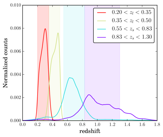
Figure 1 shows the redshift distributions for the lens and source
bins utilized in this analysis. For each lens bin, we measure the
galaxy clustering and the galaxy-galaxy lensing signals using the
estimators defined next. The correlation functions have been estimated
using the code TreeCorr444https://github.com/rmjarvis/TreeCorr
(Jarvis et al., 2004).
3.1.1 Angular Clustering –
On the galaxy clustering side, we compute the angular correlation function for each redshift bin using the minimum variance estimator of Landy & Szalay (1993),
| (11) |
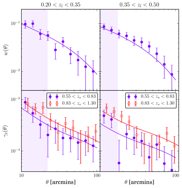
where is the angular separation in the sky, and DD, DR and RR are data-data, data-random and random-random pairs of galaxies, with data and random galaxies having the exact same geometry in the sky. The resulting measurement is shown in Fig. 2. The clustering amplitude falls from to over the range arcminutes. Only scales arcminutes and above will be used in the cosmology fits (see Sec. 5.1 for details). The details of the calculation of the error or covariance matrix for will be presented in Section 3.2.

3.1.2 Tangential Shear –
On the lensing side, the observable is the tangential shear, i.e., the shear of the source galaxy which is perpendicular to the projected line joining the lens and source galaxies. For a given lens-source pair () this is given by
| (12) |
where and are the two components of shear measured with respect to a cartesian coordinate system with origin in the lens galaxy, and is the position angle of the source galaxy with respect to the horizontal axis of the cartesian coordinate system. Since the intrinsic ellipticity of individual source galaxies is much larger than the weak lensing shear, it is necessary to average over many such lens-source pairs. For our measurements, we compute the average in angular separation bins, , so that
| (13) |
where the tangential shear for each lens-source pair, , is weighted by a factor as follows:
| (14) |
where is the shape noise intrinsic to each background galaxy, and is the error derived from the shape measurement. The weights corresponding to the shear catalogs used in this work are computed and described in Jarvis et al. (2015). In order to correct for possible geometric and additive shear systematic effects, we compute the tangential shear around random lenses and subtract this from the galaxy lensing signal (as in Clampitt et al. (2016)). The result is shown in the lower panels of Fig. 2, over the same range of scales as for . For each lens bin we show the tangential shear using the two source bins.
3.2 Covariances
Our measurements of and are correlated across angular and source redshift bins. The joint covariance for all the measurements corresponding to each lens redshift bin is estimated from jackknife (JK) resampling, using the following expression (Norberg et al., 2009):
| (15) |
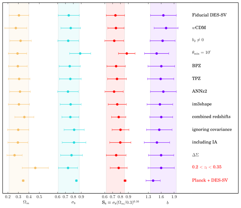
where the complete sample is split into a total of groups, is a measure of the statistic of interest in the -th bin using all JK regions excepting the -th sample, and is the mean of resamplings. Jackknife regions are obtained using the kmeans algorithm555https://github.com/esheldon/kmeans_radec run on a homogeneous random points catalog and, then, all catalogs (lenses, sources and random points) are split in JK samples. kmeans is a clustering algorithm that subdivides observations into clusters (see Appendix B in Suchyta et al. 2016 for details). By applying it to a uniform random catalog with the same sky coverage as DES-SV, we define regions that are well suited for JK subsampling. The left panel in Fig. 3 shows our JK patches created by the kmeans algorithm. The resulting covariance matrices for both lens bins are also shown in Fig. 3 (center and right panels). The covariance is strongest between points within the data vector. Note that: (i) we do not jointly fit both lens bins in the fiducial case so no covariances between lens bins are shown, and, (ii) when performing cosmology fits with the lower (higher) lens bin we only use 21 (24) data points (see Sec. 5.1). The JK covariance matrices shown in Fig. 3 contain a non-negligible level of noise. Hartlap et al. (2007) showed that the inverse of an unbiased but noisy estimator of the covariance matrix is actually not an unbiased estimator of the inverse covariance matrix. Therefore, when using a JK covariance matrix, a correction factor of should be applied to the inverse covariance, where is the number of jackknife regions and is the number of measurements (Hartlap et al., 2007). We include this correction factor in all our cosmology results. The performance of JK covariances in DES-SV has been studied separately for galaxy clustering and galaxy-galaxy lensing in Crocce et al. (2015); Giannantonio et al. (2015) and Clampitt et al. (2016), respectively. There we generally find good agreement between true covariances from simulations or theory and the JK estimates, especially at small scales. At large scales the comparison points to an overestimation of the covariance by the JK method in the lensing case. In this work we also estimate the cross-covariance between galaxy clustering and galaxy-galaxy lensing, for which we find a small positive correlation among all clustering scales and large galaxy-galaxy lensing scales – the regime where the lensing errors are no longer dominated by shape noise. This is consistent with related previous work like Mandelbaum et al. (2013), where they were able to neglect this contribution due to their different noise properties. As a check on the amount of covariance between probes, Fig. 6 also shows the result of ignoring the cross-covariance on the constraints on and . The derived cosmology shows little deviation from our fiducial results and we find that our constraints are only minimally stronger on (by about 3%) and weaker on (also 3%) with a 2% improvement on S. This shows that the impact of the correlation between probes is subdominant to the covariance within the same probe.
4 Fiducial Cosmological Constraints
| Parameter | Prior range | |
|---|---|---|
| 0.1 – 0.8 | Normalized matter density | |
| 0.04 – 0.05 | Normalized baryon density | |
| 0.4 – 1.2 | Amplitude of clustering (8 h-1Mpc top hat) | |
| 0.85 – 1.05 | Power spectrum tilt | |
| -5 – -0.33 | Equation of state parameter | |
| 0.5 – 1.0 | Hubble parameter (H0 = 100) | |
| 0.04 – 0.12 | Optical depth | |
| 1.0 – 2.2 | Linear galaxy bias | |
| -1.5 – 1.5 | Next order bias parameter | |
| -0.3 – 0.3 | Shift in photo- distribution (per source bin) | |
| -0.2 – 0.2 | Shear multiplicative bias (per source bin) | |
| -0.3 – 0.35 | Intrinsic alignment amplitude (low-z source bin only) | |
| -5 – -1 | Additive constant |
| Probes | S | ||||||
|---|---|---|---|---|---|---|---|
| DES | 0.2 0.35 | 0.73 0.12 | 0.46 0.12 | 0.77 0.11 | 0.15 | 1.60 0.31 | -1 |
| DES | 0.2 0.35 | 0.74 0.13 | 0.41 0.14 | 0.77 0.10 | 0.17 | 1.73 0.29 | -2.5 1.26 |
| DES | 0.35 0.5 | 0.74 0.13 | 0.31 0.09 | 0.74 0.12 | 0.16 | 1.64 0.30 | -1 |
| DES | 0.35 0.5 | 0.77 0.12 | 0.28 0.10 | 0.75 0.11 | 0.13 | 1.71 0.28 | -2.03 1.19 |
| DES | 0.2 0.5 | 0.76 0.10 | 0.36 0.09 | 0.78 0.09 | 0.21 | 1.52 0.28 | -1 |
| 1.60 0.27 | |||||||
| Planck | 0.83 0.01 | 0.32 0.01 | 0.82 0.02 | -0.49 | -1 | ||
| Planck | 0.98 | 0.21 | 1.210.27 | -0.6 | -1.54 | ||
| BAO + SN + H0 | 0.33 0.02 | -1.07 0.06 | |||||
| BAO + SN + H0 + DES | 0.35 0.5 | 0.710.1 | 0.32 0.02 | 0.71 0.1 | 0.01 | -1.05 0.07 | |
| DES + Planck | 0.2 0.35 | 0.84 0.01 | 0.35 0.01 | 0.76 0.02 | -0.71 | 1.30 0.13 | -1 |
| DES + Planck | 0.2 0.35 | 0.89 0.03 | 0.32 0.02 | 0.84 0.06 | -0.76 | 1.25 0.13 | -1.16 0.09 |
| DES + Planck | 0.35 0.5 | 0.84 0.01 | 0.35 0.01 | 0.76 0.02 | -0.71 | 1.41 0.17 | -1 |
| DES + Planck | 0.35 0.5 | 0.88 0.03 | 0.32 0.02 | 0.84 0.06 | -0.75 | 1.36 0.14 | -1.14 0.09 |
| DES + Planck + | 0.35 0.5 | 0.86 0.02 | 0.31 0.01 | 0.84 0.03 | -0.81 | 1.74 0.28 | -1.09 0.05 |
| BAO + SN + H0 |
In this section we present our fiducial DES-SV cosmological constraints from a joint analysis of clustering and galaxy-galaxy lensing. The data vector consists of and the two measurements for the redMaGiC bin (see Fig. 2), over angular scales of 17-100 arcminutes. We chose this lens bin as our fiducial, as we estimate greater contamination from systematic errors, on both the clustering and lensing side, for the redMaGiC bin (see Section 5.5 and Clampitt et al. (2016)). To compute the model we use CAMB (Lewis et al., 2000; Howlett et al., 2012) and Halofit (Smith et al., 2003; Takahashi et al., 2012) for the linear and non-linear matter power spectra, respectively. Because the accuracy of Halofit can be confirmed only to 5% for certain CDM models, we have checked that using the Cosmic Emulator, a more precise modelling scheme for the nonlinear dark matter power spectrum (1% to Mpc-1, Lawrence et al. 2010) would only affect our results at the level of 5% down to . We use the CosmoSIS package666https://bitbucket.org/joezuntz/cosmosis (Zuntz et al., 2015) as our analysis pipeline and explore the joint posterior distribution of our cosmological (and nuisance) parameters using the multi-nest MCMC algorithm of Feroz et al (2009), with a tolerance parameter of 0.5 and an efficiency parameter of 0.8. Our cosmological parameters and priors are summarized in Table 1 and described in greater detail next in this section. In the fiducial case, we have included two nuisance parameters per source bin (one for errors in the photo- distribution and one for biases in the shear calibration) and one nuisance parameter per lens bin (the linear bias, ; the non-linear bias, , accounting for scale dependence and stochasticity, is studied in Section 5.1), plus an additional term, , to account for potential systematic errors induced by observational effects that might induce an overall shift in the normalisation of the amplitude of (see Section 5.5). The full set of nuisance parameters and their priors are listed in the lower half of Table 1 and summarized below.
-
•
Photometric redshift calibration: For each source bin , we marginalize over a photo- bias parameter, , defined such as . In Bonnett et al. (2015), it was found that a single additive parameter for the photo- distribution with a Gaussian prior centered on zero with a dispersion of 0.05, was sufficient to account for any statistical bias on and hence within the degree of statistical error expected for the SV catalogs.
-
•
Shear calibration: For each source bin , we marginalize over an extra nuisance parameter , to account for the shear calibration uncertainties, such that , with a Gaussian prior with mean 0 and width 0.05, as advocated in Jarvis et al. (2015).
-
•
Additive constant: We marginalize over an additive constant parameter, , in the galaxy angular correlation function: . This parameter accounts for possible systematics arising from variations in observing conditions across the field, stellar contamination and masking (Ross et al., 2011), which we also test for in the next section.
| Probes | ||||||
|---|---|---|---|---|---|---|
| DES (CDM) | 0.2 0.35 | -3.41 0.84 | ||||
| DES (CDM) | 0.2 0.35 | -3.42 0.83 | ||||
| DES (CDM) | 0.35 0.5 | -3.57 0.81 | ||||
| DES (CDM) | 0.35 0.5 | -3.49 0.81 | ||||
| DES + Planck (CDM) | 0.2 0.35 | -3.62 0.82 | ||||
| DES + Planck (CDM) | 0.2 0.35 | -3.62 0.82 | ||||
| DES + Planck (CDM) | 0.35 0.5 | -3.44 0.87 | ||||
| DES + Planck (CDM) | 0.35 0.5 | -3.43 0.85 |
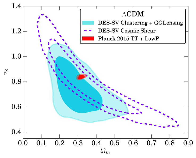
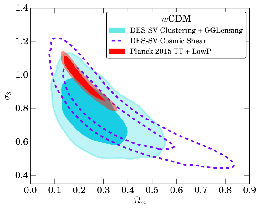
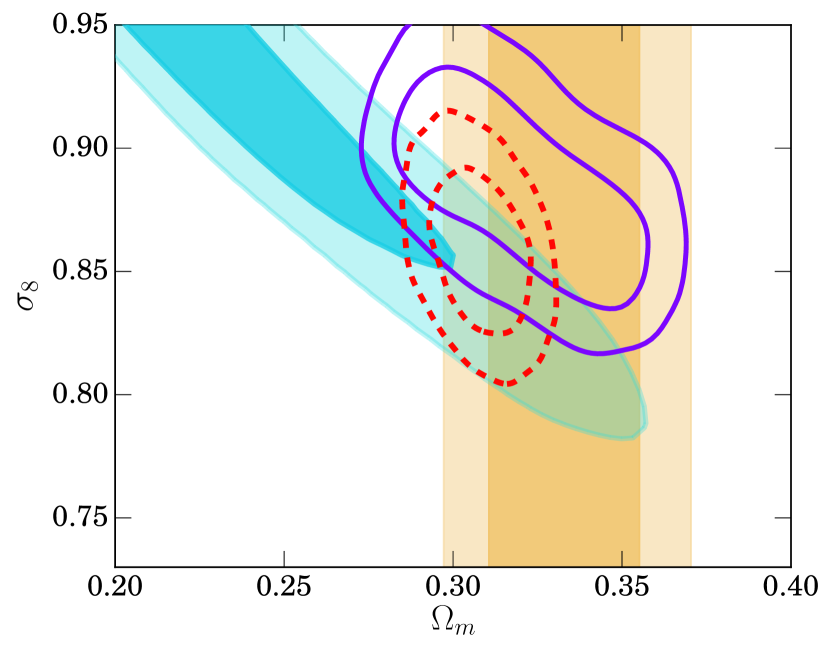
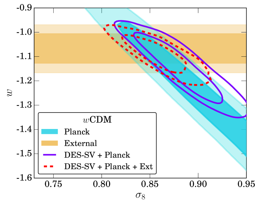
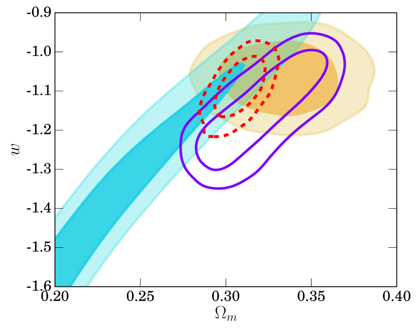
The resulting constraints in the and plane are shown in Fig. 5. The 2D contours are centered around and , and marginalizing out the other parameter we find the following 1D constraints: and . Comparing to measurements from Planck (The Planck Collaboration et al., 2015) and DES Cosmic Shear (The Dark Energy Survey Collaboration, 2015) alone, we are consistent at the or better level. We combine results from the two experiments in Section 6. In addition, we see the same direction of degeneracy between these two parameters as with cosmic shear, although the degeneracy is not quite as strong with and . We also include , the dark energy equation of state parameter, as an additional free parameter in Fig. 5. We found that the DES-SV data alone was unable to provide strong constraints on and obtained . However, compared to Planck (red contours), the DES-SV constraints on and are degraded far less when is introduced as a free parameter. Also, we note that the preference for values is determined by our choice of prior on ; we require , so the prior volume covered by is greater than and in the absence of a strong constraint on , values of are favored. Table 2 contains a more detailed summary of our findings for this fiducial setup, assuming either a CDM or CDM cosmology. In addition to DES and , we show results combined with Planck. Table 2 also shows results for our lower redshift lens bin, . For these results we vary only the cosmological parameters and where noted (in addition to the nuisance parameters described in the present and following sections). When combined with constraints from Planck, we also allow the optical depth, , to vary as well, since the CMB has additional sensitivity to physics that is only weakly captured by large scale clustering at late times. Table 3 shows the constraints on the nuisance parameters related to photo- and shear calibration described above. In the following section, we will study the robustness of these results under changes in the configuration of the data vector and the systematics modelling.
5 Robustness of the results
In this section, we describe the suite of tests performed to check that our conclusions are unbiased with respect to errors in the shear and photo- calibrations, intrinsic alignments, survey geometry, choice of angular scales and theoretical modelling of the data vectors. The results in this section are displayed in Fig. 6, for the parameters we are most sensitive to in this work: . The different rows correspond to the different tests described in this section or in the Appendix, where we check the results from a different lensing estimator. Despite the changes in the photo- algorithms, the shear catalogs, the weighting of the lens-source pairs, non-linear bias modelling and choice of scale, our estimates for these cosmological parameters in Fig. 6 usually remain within 1- of the fiducial constraints. A number of systematics that are unique to the measurement of the tangential shear such as the calibration of galaxy ellipticities, the effect of different shear calibration pipelines, null detection of the lensing B mode and effect of photo- errors in the lens and source catalogs on the measurement have already been accounted for in Clampitt et al. (2016), so we do not present tests for these effects again. For more information on tests of the shear pipeline, we refer the reader to Jarvis et al. (2015) while Bonnett et al. (2015) contains extensive tests of the photo- calibration algorithms. We also check for possible systematics introduced by the effects of survey geometry, depth and varying observing conditions in the survey following the techniques in Crocce et al. (2015). Our analysis pipeline accounts for the effect of a number of systematics which are folded into our final constraints on cosmology. To first order, these nuisance parameters are responsible for altering the amplitude of and , and so are strongly degenerate with one another. As a result, we were unable to constrain these parameters beyond their prior distributions and the results in Table 3 show that the posterior distributions of the nuisance parameters no more informative than the priors. To determine which of these most affect our results, we have analysed each of these systematics individually by running chains in four scenarios: no systematics, shear calibration only, photo- errors only, full weak lensing systematics but no constant offset in w(), and shear calibration with photo- errors (our fiducial set up). We found that including an additive constant to was responsible for the greatest decrease in precision on the 1D marginalized constraints on , with the 1- error on increasing by as much as 17% compared to the no systematics case. However, was much less affected with a difference below 3%. In comparison, accounting for photo- errors with an additional two free parameters in the distribution increased the error on both parameters by about 8%. The change from including two shear calibration parameters was smaller still, with only a 3% reduction in precision for and 5% for relative to the no systematics case. We also found small changes to the best fitting values, well within the 1- confidence interval, as expected from Fig. 6.
5.1 Choice of scales
There are several reasons to limit the range of scales that we consider in our analysis. The large scale cutoff is set by the size of the SV patch and how well the geometry of the region can be modelled; we found that our jackknife estimates of the covariance matrix overestimated the covariance matrix obtained from 50 independent N-body simulations above (see Fig 5, Clampitt et al. 2016). On small scales, we are limited by how well we can model the nonlinear clustering of matter and of redMaGiC galaxies. Galaxy formation preferentially occurs in high density environments within dark matter halos and is subject to a number of complex baryonic processes; these are not captured in our model predictions for the mass power spectrum and potentially introduce a non-trivial bias between the dark matter and the galaxies. This is particularly important for the tangential shear, which contains a mixture of small and large scale information; i.e. imposing a sharp cutoff in angular scale does not completely eliminate the effect of scales below that cutoff (Mandelbaum et al., 2013). On small enough scales, we expect to observe effects such as stochasticity, non-local bias and scale dependence. These could invalidate the linear bias model used in our analysis.
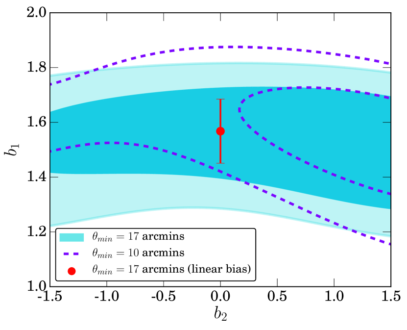
In this section, we present simulation based tests to determine the smallest scales for which the linear bias model and perturbation theory model of McDonald (2006) are valid. We use a mock catalog designed to reproduce the properties of the DES-SV survey. The catalog is based on an N-body simulation (c-400; see also Mao et al. (2015); Lehmann et al. (2015)) run with the L-Gadget code, a variant of Gadget (Springel, 2005). The simulation has a box size of 400 Mpc with 20483 particles and a force resolution of 5.5 kpc. Halo catalogs were generated with the Rockstar halo finder (Behroozi et al., 2013a) and the Consistent Trees merger tree builder (Behroozi et al., 2013b). A galaxy catalog was produced using an abundance matching technique, as described in Reddick et al. (2013) and Lehmann et al. (2015), with halos ranked according to the peak halo velocity and assigned a luminosity from the Blanton et al. (2003) luminosity function, using a scatter of 0.2 dex. Snapshots from the simulation were combined into a lightcone with the same footprint as the DES-SV region. Galaxy colors were assigned using the empirically derived relationship between luminosity, projected distance to the fifth nearest neighbor galaxy, and galaxy SED (this method for assigning colors has been used in previous generations of catalogs, see e.g. Cunha et al. 2012; Chang et al. 2015). Photometric errors were added to match the depth distribution of DES-SV galaxies. The redMaGiC algorithm was run on the lightcone, using the same technique as applied to the DES-SV data and this produced a mock redMaGiC catalog. The redMaGiC color model is retuned to the simulations before identifying these galaxies, but was found to have similar properties to that seen in the data. We find that the clustering properties of the redMaGiC galaxies in this catalog are consistent with those measured in DES-SV data. From the mock catalog, we have measured in the same bins in redshift, 0.2 0.35 and 0.35 0.5, from . Our covariance matrix is calculated from a jackknife resampling of the catalog as described in Section 3.2. We test our bias modelling by making two cuts in angular scale at and , corresponding to Mpc and Mpc, because we expect the bias to transition between its large scale asymptotic limit to scale dependence somewhere in this regime for the galaxy type that we consider. We fit both a linear and a quasilinear bias model with two free parameters, and , as described in Section 2.1 to the simulated while holding the cosmological parameters fixed to the value of the N-body simulation. Note that the effect of the shot noise parameter, , on is negligible on our scales of interest so we do not include it in our tests. Figure 7 shows the recovered biases when all the cosmological parameters are fixed at the simulation values for the fiducial lens bin of 0.35 0.5. The measured is insensitive to the value of when a minimum angular scale of is chosen (cyan filled contour) and we are simply recovering our prior distribution on . When we change the minimum scale to (purple dashed contour), there is a 1- preference for a non-zero value. Using a linear model of biasing (Fig. 7; red point) with the same fixed cosmology set up, we find that we recover the same value of as in the non-linear case. We obtain similar results for the low- lens bin, except that the minimum scale cutoff is now at for to be well modelled by a linear bias. Figure 7 demonstrates that our choice of using a linear bias up to these angular scales for the redMaGiC sample should not affect our ability to constrain cosmology. Based on these results, we can conclude that applying a linear bias model with () for the high (low-) lens bin will not bias our results in the presence of scale dependent non-linear biasing. As an additional check, we have also rerun our fiducial analysis with as an additional free parameter. For these fits, we obtained = 0.32 0.10, = 0.73 0.13, and , which is consistent with our fiducial results. For the shear catalogues, Jarvis et al. (2015) identified as the angular scale in the shear auto correlation function at which the additive errors contribute to half of the total forecasted error on the measurement of or about %. Although it is expected that position-shear correlations are less sensitive to additive systematics in the shear, we only consider angular scales even for the tests of the bias model above. This cutoff is well outside of the minimum scales considered in our cosmological analysis which use at most .
5.2 Photo- systematics
Since DES-SV is an imaging survey, the quality of our constraints rely heavily on being able to robustly calibrate the photometric redshifts of the lens and source galaxy samples. However, because does not use radial information, apart from the selection function, it is relatively insulated from photometric errors compared to the full 3D correlation function. Furthermore, because the photometric error in the lens redMaGiC sample is so small (Rozo et al., 2015b), the potential systematic errors in the cosmology analysis are dominated by the photometric redshifts of the source galaxy sample.
We deal with photometric redshift systematics in two different ways. First, we follow the recommendations of Bonnett et al. (2015) and define an additional photo- bias parameter for each source bin, , as:
| (16) |
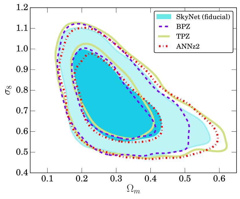
where is a free parameter with a Gaussian prior of width 0.05 to be constrained during the fitting process. The width of the prior is set to be consistent with Bonnett et al. (2015), where it was found that the difference between photometric and spectroscopic estimates of the redshift of the training samples that most closely resemble our shear catalogs have a relative mean bias with a Gaussian dispersion of 0.05. This method was also used in the DES-SV Cosmic Shear Cosmology paper (The Dark Energy Survey Collaboration, 2015). We found that introducing an additional photo- bias parameter for each source bin increases our uncertainty by, at most, 8% compared to the constraints we would have if we did not fit for any systematic parameters. In addition, we check that our constraints are robust to our choice of photo- algorithm. Our fiducial shear catalogs use photometric redshifts derived from the SkyNet algorithm (Graff et al., 2014; Bonnett et al., 2015), and we have repeated our analysis by using the redshift distribution given by three other photo- codes studied in Bonnett et al. (2015), namely BPZ, TPZ and ANNz2. For this test, we assume a CDM cosmology and allow the cosmological parameters to vary. In addition, we also fit for the usual systematic parameters, for the photo- bias and for the multiplicative bias in the shear calibration and the same prior distributions. The resulting constraints in Fig. 8 (and 6) show that our results are insensitive to the choice of the photo- algorithm. Interested readers should refer to Bonnett et al. (2015) for a full discussion of the photo- methods considered and the systematics modelling that we have only summarized here.
5.3 Shear calibration systematics
Here we present our approach to modelling a possible residual error in the shear calibration. For the interested reader, the full details of the production and testing of the shear catalogs used in this analysis are given in Jarvis et al. (2015). Similar to the photometric redshift case, we deal with potential shear calibration systematics on two fronts. Firstly, we include an extra nuisance parameter for the shear calibration, , as:
| (17) |
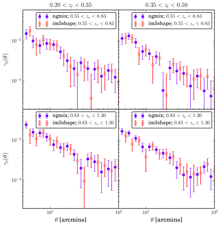
with a Gaussian prior, , with mean 0 and width 0.05, for each source bin in our analysis as recommended in Jarvis et al. (2015). Contamination from additive errors in the shear estimation are expected to be minimal for galaxy-galaxy lensing, because of the azimuthal symmetry of the lens system. Including an additional parameter for the shear calibration degrades our constraints by, at most, 5%, compared to all systematic parameters being ignored or set to fixed values. Secondly, galaxy images in the DES-SV region were analyzed with two pipelines, ngmix and im3shape. Jarvis et al. (2015) showed that they both produced consistent results that satisfied the SV requirements for weak lensing, i.e. that less than half of the forecasted error on (about 3%) originates from systematics in the measurement of the shear. Although we have chosen to use the ngmix catalog for our analysis, we have also rerun the analysis pipeline on the im3shape catalog to check that our results are not sensitive to the shear catalog used (see Fig. 13 for a comparison of lensing measurements using the two shear pipelines). We found that the cosmological parameters varied imperceptibly when the im3shape catalog was used instead of ngmix. This is demonstrated in Fig. 6.
5.4 Intrinsic Alignments
Correlations between the intrinsic shapes and orientations of lensing sources, known as “intrinsic alignments” (IA), are one of the most significant astrophysical sources of uncertainty in weak lensing measurements (see Troxel & Ishak 2015; Joachimi et al. 2015 for recent reviews). Although typically considered in the context of shear-shear correlations, IA can also contaminate galaxy-galaxy lensing measurements due to uncertainties in photo- estimates which lead to overlap in the true lens and source distributions (see Fig. 1). The intrinsic shapes of sources can be correlated with the positions of lenses at the same redshift (Blazek et al., 2012). In general, the contamination from IA reflects the (potentially nonlinear) relationship between large-scale structure and galaxy shapes, as well as the clustering of lenses and physically associated sources. However, observational evidence (e.g. Joachimi et al. 2011; Blazek et al. 2011; Singh & Mandelbaum 2015) indicates that the dominant IA contribution is likely from elliptical (pressure-supported) galaxies, for which the IA component is linearly related to the large-scale tidal field. This “tidal alignment” paradigm (Catelan et al., 2001; Hirata & Seljak, 2004; Blazek et al., 2015) was recently used to mitigate IA in the DES-SV Cosmic Shear Cosmology analysis (The Dark Energy Survey Collaboration, 2015). In this work, we consider scales on which the clustering of lens-source pairs is negligible (see Clampitt et al. 2016 for further discussion). In this regime, tidal alignment predicts that the fractional IA contamination to the lensing signal is nearly scale-invariant. Both the IA and lensing are sourced by the same matter power spectrum, even in the presence of nonlinear evolution, and we find that the different line-of-sight weighting for IA and lensing (e.g. Eq. 3) leads to negligible relative scale-dependence in angular correlations. We thus account for the potential impact of IA in our analysis by including an additional term that modifies the amplitude of the tangential shear, such that . We place a Gaussian prior on of 8% % for the lower redshift source bin. The higher redshift source bin is sufficiently separated from the redshift of the lenses that the potential IA contamination is negligible. Our priors on the expected IA contamination are calculated from the overlap in lens and source redshift distributions and assume an IA amplitude consistent with the constraints found in the cosmic shear analysis of the same sources on the DES-SV patch (The Dark Energy Survey Collaboration, 2015). Potential IA contamination in the galaxy-galaxy lensing measurement is discussed further in Clampitt et al. (2016). We do not observe a significant detection of IA contamination beyond the prior imposed; we find that % for the low redshift sources with % for the higher source bin. Including IA only affects the cosmology results by, at most, inducing a 3% shift towards a lower value of compared to the fiducial case without IA, as shown in Fig 6. For , the change was much smaller, with a fractional shift of less than a percent. Because the inclusion of IA contamination has a negligible effect on our results, compared to the statistical errors, we do not include IA modelling for our fiducial analysis.
5.5 Impact of observing conditions
Photometric galaxy surveys such as DES are affected by time-dependent fluctuations in observing conditions that may impact the galaxy catalogs. There are a number of effects that can modulate the detection efficiency of galaxies and cause density variations across the survey footprint. In this section we follow the approach of Crocce et al. (2015) and consider single-epoch properties that affect the sensitivity of the survey and hence may affect the galaxy clustering and galaxy-galaxy lensing observables. We use projected HEALPix777http://healpix.sf.net (Górski et al., 2005) sky maps (with resolution nside=4096) in bands for the following quantities:
-
•
depth: mean survey depth, computed as the mean magnitude for which galaxies are detected at .
-
•
FWHM: mean seeing, in pixel units, computed as the full width at half maximum of the flux profile.
-
•
airmass: mean airmass, computed as the optical path length for light from a celestial object through Earth’s atmosphere (in the secant approximation), relative to that at the zenith for the altitude of CTIO.
-
•
skysigma: mean sky background noise, computed as the flux variance per amplifier in chip of the CCD.
-
•
USNO: mean stellar density, as measured by the USNO-B1 stellar catalog (Monet et al., 2003) with B magnitude brighter than 20 to ensure constant depth across the field.
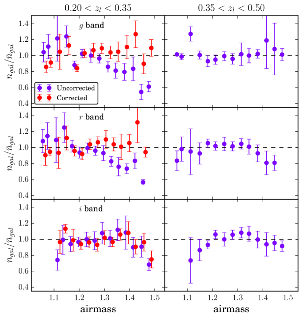
See Leistedt et al. (2015) for a full description of these maps. We study the density of redMaGiC galaxies in the two lens bins as a function of each of these quantities that can potentially result in systematic effects. To ensure the data is free of such systematics, we require the galaxy density to be uncorrelated with the observed depth, FWHM, airmass, skysigma and USNO, otherwise we apply a correction to remove the dependency. Among the five quantities for each band and each lens bin considered here, we only find a significant correlation in the low- bin with airmass in the and DES bands. This trend is demonstrated in Fig. 9, which shows the redMaGiC galaxy density as a function of airmass in , and bands for the two lens bins. In order to correct for this correlation, we weight galaxies according to the inverse of a linear fit to the observed trend of airmass in the band. This procedure is similar to that applied in Ross et al. (2012, 2014) to correct for systematic relationships with stellar density and airmass. The corrected results are shown in Fig. 9, where we see that the band weighting also corrects the trend in the band, as expected given the correlation present among the airmass maps in the and bands. In addition to the weighting correction described above, we have also applied the procedure used in Crocce et al. (2015), in which galaxy and systematics maps are cross-correlated and used to correct the galaxy correlation functions. At the galaxy clustering level, the two approaches yield consistent results. Furthermore, in both cases the correction is compatible with an additive constant in the angular galaxy clustering signal. Nonetheless, we introduce an additive constant as a systematics parameter in the corrected measurement of as outlined in Section 4 to deal with any residual systematic effects. This is marginalized over in the cosmological analysis according to the prior defined in Table 1. On the other hand, the impact of the airmass correction in the galaxy-galaxy lensing observables is not significant given the statistical power of these observations in DES-SV. As opposed to Crocce et al. (2015) we do not find the depth and FWHM maps to be relevant for our lens sample, mainly because redMaGiC galaxies are much brighter than the DES main galaxy sample (Benchmark) considered in that work. On the other hand, correlations between airmass maps and galaxy positions were not found to be a significant systematic in Crocce et al. (2015), while for redMaGiC galaxies in the low- lens bin, this was the only observing condition with a substantial impact on clustering. While Crocce et al. (2015) includes all types of galaxies, the redMaGiC selection process preferentially chooses red galaxies as described in Section 3. It is plausible that these galaxies are more affected by airmass, via their sensitivity to atmospheric extinction. At high airmass, the filter bandpasses shift to the red and the RedMapper color selection, in which redMaGiC relies, do not compensate for this. The effect is more important for the bluer DES bands and (Li et al., 2016), and the key spectral features of red galaxies, like the 4000Å break, fall in a bluer window of the filter set at lower redshifts, and hence the effect of atmospheric extinction is enhanced for our low- lens bin. In the following subsection, we present cosmology results with the low- lens bin after correcting for the correlation with airmass.
5.6 Low- lens bin results
In this section we present the cosmology results obtained for the low- redMaGiC lens bin (), described in Section 3.1 and for which measurements are shown in Fig. 2. For this bin, a significant correlation of the galaxy density with airmass was found and corrected for in Section 5.5. The photo- and shear systematics treatment in the cosmology pipeline is equivalent to that of the fiducial lens bin and we use these results as another robustness check for the cosmological analysis performed in this work. The cosmological constraints obtained from these measurements are shown in Fig. 6 and Table 2, and the constraints on and from the combination with the fiducial high- lens bin are shown in Fig. 10. For most of the parameters, these lower redshift lenses are in agreement with our fiducial setup, but shows a preference for higher values after correcting for the observing conditions described in Section 5.5. Still, the results for both lens bins are within 1 of each other.
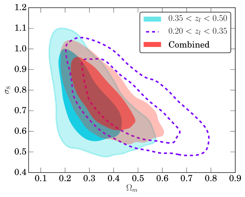
Having confirmed that the results from both the low and high redshift lens bins are consistent, we explore fitting them jointly in the same analysis pipeline to improve our constraints on cosmology. The covariance between lens bins may include a contribution from shape noise in the shear catalog. We estimate this contribution by introducing a random direction to the measured ellipticities before calculating the tangential shear. This is performed 300 times to obtain a jackknife estimate of the shape noise across lens and source bins. We then add the shape noise as an off-diagonal component to the covariance matrix between lens bins with the diagonal components being the usual JK covariance matrices used for individual fits. We find that the marginalized constraints are and , which show very little improvement on our fiducial results. However, the constraint on S, where is chosen to be perpendicular to the degeneracy direction in the - plane, shows a reduction in the error, from S ( = 0.16; high- lenses only) to S (; all lenses). These values of , and S8 are shown in Fig. 6. We do not however consider this arrangement as our ‘fiducial’ model, leaving joint constraints to future work with additional survey area.
6 Discussion
We have presented our baseline cosmological results from DES data in Section 4, assuming a flat CDM model in Figure 5 and a flat CDM model in Figure 5. Our results for the marginalized mean parameter values are contained in Table 2 for each lens bin, with and without external data sets. We also show results for each of the nuisance parameters used in our fits in Table 3.
6.1 External Datasets
We performed a joint analysis of our measurements with the Planck 2015 temperature and polarization auto and cross multipole power spectra, and . Specifically, we use the full range of from 29 2509 and the low- polarization data from 2 29, which we denote as Planck (TT-lowP). The inclusion of the maps allows for stronger constraints on which in turn affects , the primordial power spectrum amplitude. We have also chosen this configuration to allow for an easy comparison with the DES-SV Cosmic Shear Cosmology paper (The Dark Energy Survey Collaboration, 2015). The constraints from only using this configuration of Planck data when assuming a CDM model are shown as the red contours in Fig. 5. With the inclusion of the DES and measurements, we were able to improve on the constraints on and from just Planck alone, which prefers and . This is in part because DES provides modest constraints on which help break the degeneracy between and in the CMB. In addition, the Planck dataset prefers higher values of and than the DES data, such that in combination, the two probes carve out a smaller area in parameter space. This produces strong constraints on when the two datasets are combined. In combination with Planck, we find that , and . Fig. 11 shows the result of combining our measurements with additional data sets beyond the CMB. The other probes that we consider are BAO measurements from 6dF (Beutler et al., 2011), BOSS (Anderson et al., 2014; Ross et al., 2015), Supernova type Ia measurements (Betoule et al., 2014) and direct measurements of (Efstathiou,, 2014). These data sets alone give constraints of and and no constraint on (the posterior distribution on is fully informed by the prior). Combining these data sets with DES and the CMB gives an improvement in precision and strengthens our results to and and .
6.2 Comparison with DES cosmic shear
The Dark Energy Survey Collaboration (2015) measured the 2-point shear correlations, for the same DES-SV area and source catalogs. The best fitting cosmological parameters in that work were and . Figs. 5 and 5 show the constraints from the analysis presented in this work on those parameters together with constraints from the shear 2-point correlations for the CDM and CDM models, respectively. There is very good agreement between the two analyses and a similar degeneracy direction in the – plane as well. The shape of the contours for the two methods in Fig. 5 is somewhat different, with the cosmic shear contours being more elongated. We find that the slope in the derived parameter S is 0.16 for and instead of 0.478 for cosmic shear. In part because the covariance between and is weaker, the constraints on each parameter are slightly stronger for the and case. The results in this analysis are less sensitive to errors in the lensing shear and redshift distribution of source galaxies since these do not impact at all, and additive errors in the shear cancel out of at lowest order. On the other hand, cosmic shear measurements are unaffected by errors in the galaxy biasing model and systematic errors in the measurement of galaxy clustering. Furthermore, the derived parameter S8 is better constrained by DES cosmic shear. While there is significant complementarity in the two measurements, they are also correlated because of the shared source galaxies. The combination of all three 2-point functions taking into account covariances is an important next step in the cosmological analysis of DES.
6.3 Comparison with the literature
A number of previous papers have considered the combination of and as probes of cosmology. Mandelbaum et al. (2013) perform an analysis with SDSS DR7 using luminous red galaxies as the lenses and derive comparable constraints. With some cosmological parameters fixed, Mandelbaum et al. (2013) used a combination of three lensing and angular clustering measurements in the redshift range 00.5 to obtain and . Several details of our analysis differ from Mandelbaum et al. (2013), but the broad approach of employing a quasilinear analysis on large scales is similar and the results are consistent. Cacciato et al. (2013) also measure the tangential shear and angular clustering from SDSS DR7 data, but differ in that they include small scale clustering and consider a subset of the galaxy samples used by Mandelbaum et al. (2013). They adopt a halo model approach which allows them to extend their analysis to much smaller scales than Mandelbaum et al. (2013), at the expense of requiring additional free parameters and model ingredients that are calibrated with simulations. With this small scale approach, Cacciato et al. (2013) obtain and , again consistent with our derived constraints. Similarly, More et al. (2015) use a halo model approach to calculate the joint likelihood using galaxy clustering, galaxy-galaxy lensing and galaxy abundance for the CMASS sample observed in BOSS using CFHTLenS sources. They report that and . Applying an HOD model motivates the inclusion of small scale information in their cosmology fits. In terms of number density and typical halo mass, the CMASS galaxies used by More et al. (2015) are closer to our redMaGiC sample than the LRGs in Mandelbaum et al. (2013), but they all derive consistent cosmological constraints.
7 Conclusions
In this paper we have presented cosmological constraints from the combination of large-scale structure and weak gravitational lensing in the Dark Energy Survey. Using a contiguous patch of 139 sq. deg. from the Science Verification period of observations, we have placed constraints on the matter density and the amplitude of fluctuations in the Universe as and , respectively. We also present joint constraints with CMB measurements from Planck, and additional low-redshift datasets. When allowing for a dark energy equation of state parameter different to the CDM value of , we find DES data improve the constraints on as well as . We leave a full tomographic analysis with multiple lens bins and a joint analysis with cosmic shear for future DES releases. We have assessed the robustness of our results with respect to several variations in the choice of data vector, modelling and treatment of systematics. In particular, the results are stable under the use of two different shear catalogs, four different photo- codes and two different estimators of the lensing signal. They also show consistency with the fiducial results when using a different lens bin, a different selection of angular scales or when adding a nonlinear galaxy bias parameter. The DES-SV region comprises only 3% of the eventual survey coverage, and we expect to greatly improve on our constraining power with future data releases. For now, the analysis presented in this paper is complementary to and provides a useful consistency check with the analysis of the shear 2-point function presented in The Dark Energy Survey Collaboration (2015). These analyses validate the robust modelling of systematic errors and galaxy bias, as well as the exhaustive testing of the shear pipeline, photo- estimation and the redMaGiC galaxy sample selection in the Dark Energy Survey.
Acknowledgments
We are grateful for the extraordinary contributions of our CTIO colleagues and the DECam Construction, Commissioning and Science Verification teams in achieving the excellent instrument and telescope conditions that have made this work possible. The success of this project also relies critically on the expertise and dedication of the DES Data Management group. Funding for the DES Projects has been provided by the U.S. Department of Energy, the U.S. National Science Foundation, the Ministry of Science and Education of Spain, the Science and Technology Facilities Council of the United Kingdom, the Higher Education Funding Council for England, the National Center for Supercomputing Applications at the University of Illinois at Urbana-Champaign, the Kavli Institute of Cosmological Physics at the University of Chicago, the Center for Cosmology and Astro-Particle Physics at the Ohio State University, the Center for Particle Cosmology and the Warren Center at the University of Pennsylvania, the Mitchell Institute for Fundamental Physics and Astronomy at Texas A&M University, Financiadora de Estudos e Projetos, Fundação Carlos Chagas Filho de Amparo à Pesquisa do Estado do Rio de Janeiro, Conselho Nacional de Desenvolvimento Científico e Tecnológico and the Ministério da Ciência e Tecnologia, the Deutsche Forschungsgemeinschaft and the Collaborating Institutions in the Dark Energy Survey. The DES data management system is supported by the National Science Foundation under Grant Number AST-1138766. The DES participants from Spanish institutions are partially supported by MINECO under grants AYA2012-39559, ESP2013-48274, FPA2013-47986, and Centro de Excelencia Severo Ochoa SEV-2012-0234, some of which include ERDF funds from the European Union. The Collaborating Institutions are Argonne National Laboratory, the University of California at Santa Cruz, the University of Cambridge, Centro de Investigaciones Energeticas, Medioambientales y Tecnologicas-Madrid, the University of Chicago, University College London, the DES-Brazil Consortium, the Eidgenössische Technische Hochschule (ETH) Zürich, Fermi National Accelerator Laboratory, the University of Edinburgh, the University of Illinois at Urbana-Champaign, the Institut de Ciències de l’Espai (IEEC/CSIC), the Institut de Física d’Altes Energies, Lawrence Berkeley National Laboratory, the Ludwig-Maximilians Universität and the associated Excellence Cluster Universe, the University of Michigan, the National Optical Astronomy Observatory, the University of Nottingham, The Ohio State University, the University of Pennsylvania, the University of Portsmouth, SLAC National Accelerator Laboratory, Stanford University, the University of Sussex, and Texas A&M University.
Appendix A Excess Surface Density
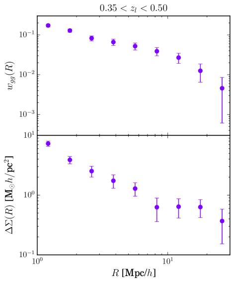
In this section, we present complementary cosmology results obtained for the fiducial redMaGiC lens bin () by using the excess surface density, as a proxy for the galaxy-galaxy lensing signal of redMaGiC galaxies. For this purpose, we define another lensing estimator that optimally weights each lens-source pair of galaxies depending on the line-of-sight distance separating them. This effectively downweights pairs of galaxies which are very close and for which we expect a small lensing efficiency. The observable is estimated from the measured shapes of background galaxies as
| (18) |
where the summation goes over all the source galaxies in the radial bin , around all the lens galaxy positions, and the weight factor for the -th galaxy is given by
| (19) |
Note that, in contrast with , for we bin source galaxies according to radial distance in the region around each lens galaxy, instead of angular scale . In order to estimate distances, we assume a flat CDM model with . The weighting factor is computed as a function of lens and source redshifts for the assumed cosmology as
| (20) |
where for and is the angular diameter distance. We have checked that changes in the assumed cosmology have little impact in the estimation of so that they are not relevant for the analysis presented in this work (see also Mandelbaum et al. 2013). Finally, just as we do with tangential shear measurements, our final estimator involves subtracting the contribution around random points, to which now we assign redshifts randomly drawn from the real lens redshift distribution. Figure 12 shows the clustering and the galaxy-galaxy lensing signals, the latter using the alternative estimator, both binned according to projected radial distance around lenses. In this case, we use all source galaxies available in the ngmix fiducial shear catalog and we weight each lens-source galaxy pair according to their individual photometric redshifts so that nearby pairs for which we expect a small lensing efficiency are effectively downweighted. For the angular clustering, essentially the same dataset is used in Fig. 12 as for our fiducial results pictured in Fig. 2. Thus, the two plots are very similar, with the main difference being the range of scales shown on the x-axis. Our cosmological constraints obtained from fitting for and are shown in Fig. 6. These are consistent with our fiducial results, and show tighter constraints on parameters like , due to the optimal lens weighting and the larger number of source galaxies effectively used. However, we do not use this estimator as the fiducial given the larger uncertainties in the photo- modelling, which enters here on a galaxy-by-galaxy basis unlike the tangential shear which only uses the full stacked distribution. Instead, we take the conservative approach of using the tangential shear lensing measurements for the fiducial case, which has better control over the potential photo- systematic effects.
Appendix B ngmix vs. im3shape
In Section 5.3 we studied the consistency of the obtained cosmological constraints when using the two shear pipelines presented in Jarvis et al. (2015). In Fig. 13 we show the actual comparison of the lensing measurements from the two shear pipelines, for all the different lens - source bin configurations. The im3shape results are an excellent match to our fiducial measurements with ngmix (shown earlier in Fig. 2).
References
- Anderson et al. (2014) Anderson, L, et al. 2014, MNRAS, 441, 24
- Baldauf et al. (2010) Baldauf, T., Smith, R. E., Seljak, U., & Mandelbaum, R. 2010, Phys. Rev. D, 81, 063531
- Becker et al. (2015) Becker, M. R., Troxel, M. A., MacCrann, N., et al. 2015, arXiv:1507.05598
- Behroozi et al. (2013a) Behroozi, P. S., Wechsler, R. H. & Wu, H.-Y., 2013, ApJ, 762, 109
- Behroozi et al. (2013b) Behroozi, P. S., Wechsler, R. H., Wu, H.-Y., Busha, M. T., Klypin, A. A. & Primack, J. R., 2013, ApJ, 763, 18
- Benítez (2000) Benítez, N. 2000, ApJ, 536, 571 Data Analysis Software and Systems XX, 442, 435
- Betoule et al. (2014) Betoule, M, et al. 2014, A&A, 568, 22
- Beutler et al. (2011) Beutler, F., Blake, C., Colless, M., Jones, D. H., Staveley-Smith, L., Campbell, L., Parker, Q, Saunders, W, et al., 2011, MNRAS, 416, 3017
- Blanton et al. (2003) Blanton, M. R., Hogg, D. W., Bahcall, N. A., Brinkmann, J., Britton, M., Connolly, A. J., Csabai, I., Fukugita, M., et al., 2003, ApJ, 592, 819
- Blazek et al. (2011) Blazek, J., McQuinn, M., & Seljak, U., 2011, JCAP, 5, 1
- Blazek et al. (2012) Blazek, J., Mandelbaum, R., Seljak, U., & Nakajima, R, 2012, JCAP, 5, 41
- Blazek et al. (2015) Blazek, J., Vlah, Z., & Seljak, U., 2015, JCAP, 8, 15
- Bonnett et al. (2015) Bonnett, C., Troxel, M. A., Hartley, W., et al. 2015, arXiv:1507.05909
- Bonnett et al. (2015) Bonnett, C., 2015, MNRAS, 449, 1043
- Brainerd, Blandford & Smail (1996) Brainerd, T. G., Blandford, R. D., Smail, I., 1996, ApJ, 466, 623
- Carrasco Kind & Brunner (2013) Carrasco Kind, M., & Brunner, R., J., 2013, MNRAS, 432, 1483
- Cacciato et al. (2009) Cacciato, M., van den Bosch, F. C., More, S., et al. 2009, MNRAS, 394, 929
- Cacciato et al. (2013) Cacciato, M., van den Bosch, F. C., More, S., Mo, H., & Yang, X. 2013, MNRAS, 430, 767
- Catelan et al. (2001) Catelan, P., Kamionkowski, M., & Blandford, R. D., 2001, MNRAS, 320, 7
- Chang et al. (2015) Chang, C., Vikram, V., Jain, B., Bacon, D., Amara, A., Becker, M. R., Bernstein, G. & Bonnett, C. et al., 2015, Physical Review Letters, 115, 1301
- Cooray & Sheth (2002) Cooray, A., & Sheth, R. 2002, PhR, 372, 1
- Clampitt et al. (2016) Clampitt, J., Sánchez, C., Kwan, J., et al. 2016, arXiv:1603.05790
- Crocce et al. (2015) Crocce, M., Carretero, J., Bauer, A. H., et al. 2015, arXiv:1507.05360
- Cunha et al. (2012) Cunha, C. E., Huterer, D., Busha, M. T. & Wechsler, R. H., 2012, MNRAS, 423, 909
- The Dark Energy Survey Collaboration (2015) The Dark Energy Survey Collaboration, Abbott, T., Abdalla, F. B., et al. 2015, arXiv:1507.05552
- The Dark Energy Survey Collaboration (2016) The Dark Energy Survey Collaboration, Abbott, T., Abdalla, F. B., et al. 2016, arXiv:1601.00329
- de Jong et al. (2013) de Jong, J. T. A., Verdoes Kleijn, G. A., Kuijken, K. H., & Valentijn, E. A. 2013, Experimental Astronomy, 35, 25
- de Jong et al. (2015) de Jong, J. T. A., Verdoes Kleijn, G., A., Boxhoorn, D. R., Buddelmeijer, H., Capaccioli, M., Getman, F., Grado, F., Helmich, E., et al., 2015, A&A, 582, A62
- Efstathiou, (2014) Efstathiou, G, 2014, MNRAS, 440, 1138
- Erben et al. (2013) Erben, T., Hildebrandt, H., Miller, L., et al. 2013, MNRAS, 433, 2545
- Feroz et al (2009) Feroz, F., Hobson, M. P., & Bridges, M., 2009,MNRAS, 398, 1601
- Flaugher et al. (2012) Flaugher, B. L., Abbott, T. M. C., Angstadt, R., et al. 2012, SPIE, 8446, 844611
- Flaugher et al. (2015) Flaugher, B., Diehl, H. T., Honscheid, K., Abbott, T. M. C., Alvarez, O., Angstadt, R., Annis, J. T., Antonik, M. et. al, 2015, AJ 150, 150.
- Giannantonio et al. (2015) Giannantonio, T., Fosalba, P. et al. 2015, arXiv:1507.05551
- Gillis et al. (2013) Gillis, B. R., Hudson, M. J., Erben, T., et al. 2013, MNRAS, 431, 1439
- Górski et al. (2005) Górski, K. M., Hivon, E., Banday, A. J., et al. 2005, ApJ, 622, 759
- Graff et al. (2014) Graff, P., Feroz, F., Hobson, M. P., & Lasenby, A. 2014, MNRAS, 441, 1741
- Gruen et al. (2015) Gruen, D., Friedrich, O., Amara, A., et al. 2015, arXiv:1507.05090
- Guzik & Seljak (2001) Guzik, J. & Seljak, U, 2001, MNRAS, 321, 439
- Heymans et al. (2012) Heymans, C., Van Waerbeke, L., Miller, L., Erben, T., Hildebrandt, H., Hoekstra, Kitching, T. D., et al., 2012, MNRAS, 427, 146
- Hartlap et al. (2007) Hartlap, J., Simon, P. & Schneider, P. 2007, A&A, 464, 399
- Hirata & Seljak (2004) Hirata, C. & Seljak, U., 2004, Phys. Rev. D, 70, 063526
- Howlett et al. (2012) Howlett, C., Lewis, A., Hall, A., & Challinor, A. 2012, JCAP, 4, 027
- Hudson et al. (2015) Hudson, M. J., Gillis, B. R., Coupon, J., et al. 2015, MNRAS, 447, 298
- Jarvis et al. (2004) Jarvis, R. M., Bernstein, G.,& Jain, B., 2004, MNRAS, 352 338
- Jarvis et al. (2015) Jarvis, M., Sheldon, E., Zuntz, J., et al. 2015, arXiv:1507.05603
- Joachimi et al. (2011) Joachimi, B., Mandelbaum, R., Abdalla, F. B. & Bridle, S. L., 2011, A&A, 527, 26
- Joachimi et al. (2015) Joachimi, B., Cacciato, M., Kitching, T. D., Leonard, A., Mandelbaum, R., Schäfer, B. M., Sifón, C. Hoekstra, H., et al., Space Science Reviews, 193, 1
- Kaiser (1992) Kaiser, N., 1992, ApJ, 388, 272,
- Kuijken et al. (2015) Kuijken, K., Heymans, C., Hildebrandt, H., et al. 2015, MNRAS, 454, 3500
- Landy & Szalay (1993) Landy, S. D., & Szalay, A. S. 1993, ApJ, 412, 64
- Lawrence et al. (2010) Lawrence, E., Heitmann, K., White, M., Higdon, D., Wagner, C., Habib, S., & Williams, B., 2010, ApJ, 713, 1322
- Leauthaud et al. (2012) Leauthaud, A., Tinker, J., Bundy, K., et al. 2012, ApJ, 744, 159
- Lehmann et al. (2015) Lehmann, B. V., Mao, Y.-Y., Becker, M. R., Skillman, S. W. & Wechsler, R. H. 2015, arXiv:1510.05651
- Leistedt et al. (2015) Leistedt, B., Peiris, H. V., Elsner, F., et al. 2015, arXiv:1507.05647
- Lewis et al. (2000) Lewis, A., Challinor, A., & Lasenby, A. 2000, ApJ, 538, 473
- Li et al. (2016) Li, T. S., DePoy, D. L., Marshall, J. L., et al. 2016, arXiv:1601.00117
- Limber (1953) Limber, D., N., 1953, ApJ, 117, 134
- Mandelbaum et al. (2006) Mandelbaum, R., Seljak, U., Cool, R. J., et al. 2006, MNRAS, 372, 758
- Mandelbaum et al. (2008) Mandelbaum, R., Seljak, U., & Hirata, C. M. 2008, JCAP, 8, 6
- Mandelbaum et al. (2013) Mandelbaum, R., Slosar, A., Baldauf, T., et al. 2013, MNRAS, 432, 1544
- Mao et al. (2015) Mao, Y-Y, Williamson, M., & Wechsler, R. H., 2015, ApJ, 810, 21
- McDonald (2006) McDonald, P., 2006, Phys. Rev. D, 74, 103512
- Miyazaki et al., (2012) Miyazaki, S., Komiyama, Y., Nakaya, H., Kamata, Y., Doi, Y., Hamana, T., Karoji, H., Furusawa, H., et al., 2012, SPIE, 8446, 0Z
- Monet et al. (2003) Monet, D. G., Levine, S. E., Canzian, B., Ables, H. D., et al. 2003, AJ, 125, 984
- More et al. (2015) More, S., Miyatake, H., Mandelbaum, R., et al. 2015, ApJ, 806, 2
- Norberg et al. (2009) Norberg, P., Baugh, C. M., Gaztañaga, E., & Croton, D. J. 2009, MNRAS, 396, 19
- Park et al. (2015) Park, Y., Krause, E., Dodelson, S., et al. 2015, arXiv:1507.05353
- The Planck Collaboration et al. (2015) The Planck Collaboration, Ade., P. A. R et al, 2015, arXiv:1502.01589
- Reddick et al. (2013) Reddick, R. M., Wechsler, R. H., Tinker, J. L., & Behroozi, P. S., 2013, ApJ, 771, 30
- Ross et al. (2011) Ross, A., J. et al. 2011, MNRAS, 417, 1350
- Ross et al. (2012) Ross, A. J. et al. 2012, MNRAS, 424, 564
- Ross et al. (2014) Ross, A. J. et al. 2014, MNRAS, 437, 1109
- Ross et al. (2015) Ross, A. J. et al. 2015, MNRAS, 449, 835
- Rozo et al. (2015a) Rozo, E., Rykoff, E. S., Becker, M., Reddick, R. M., & Wechsler, R. H. 2015, MNRAS, 453, 38
- Rozo et al. (2015b) Rozo, E., Rykoff, E. S., Abate, A., et al. 2015, arXiv:1507.05460
- Rykoff et al. (2014) Rykoff, E. S., Rozo, E., Busha, M. T., et al. 2014, ApJ, 785, 104
- Sadeh et al. (2015) Sadeh I., Abdalla F., B., Lahav O., 2015, arXiv:1507.00490
- Seljak (2000) Seljak U., 2000, MNRAS, 318, 203
- Sánchez et al. (2014) Sánchez, C., Carrasco Kind, M., Lin, H., et al. 2014, MNRAS, 445, 1482
- Sheldon et al. (2004) Sheldon, E. S., Johnston, D. E., Frieman, J. A., et al. 2004, AJ, 127, 2544
- Sheldon (2014) Sheldon, E. S. 2014, MNRAS, 444, L25
- Sifón et al. (2015) Sifón, C., Cacciato, M., Hoekstra, H., et al. 2015, MNRAS, 454, 3938
- Singh & Mandelbaum (2015) Singh, S., & Mandelbaum, R., 2015, MNRAS, 450, 2195
- Smith et al. (2003) Smith, R. E., Peacock, J. A., Jenkins, A., et al. 2003, MNRAS, 341, 1311
- Springel (2005) Springel, V., 2005, MNRAS, 364, 1105
- Suchyta et al. (2016) Suchyta, E., Huff, E. M., Aleksic, J., Melchior, P., et al. 2016, MNRAS, 457, 786
- Takahashi et al. (2012) Takahashi, R., Sato, M., Nishimichi, T., Taruya, A., & Oguri, M. 2012, ApJ, 761, 152
- Troxel & Ishak (2015) Troxel, M. A. & Ishak, M., 2015, PhR, 558, 1T
- Tyson et al. (1984) Tyson, J. A., Valdes, F., J. F., & Mills, A. P., Jr. 1984, ApJL, 281, L59
- van Uitert et al. (2016) van Uitert, E., Cacciato, M., Hoekstra, H., et al. 2016, arXiv:1601.06791
- Velander et al. (2014) Velander, M., van Uitert, E., Hoekstra, H., et al. 2014, MNRAS, 437, 2111
- Vikram et al. (2015) Vikram, V., Chang, C., Jain, B., et al. 2015, Phys. Rev. D, 92, 022006
- Viola et al. (2015) Viola, M., Cacciato, M., Brouwer, M., et al. 2015, MNRAS, 452, 3529
- Yang et al. (2006) Yang, X., Mo, H. J., van den Bosch, F. C., et al. 2006, MNRAS, 373, 1159
- Yoo & Seljak (2012) Yoo, J., & Seljak, U. 2012, Phys. Rev. D, 86, 083504
- York et al. (2000) York, D. G., Adelman, J., Anderson, J. E., Jr., Anderson, S. F., Annis, J., Bahcall, N. A., Bakken, J. A., Barkhouser, R., et al., 2000, AJ, 120, 9
- Zuntz et al. (2013) Zuntz, J., Kacprzak, T., Voigt, L., et al. 2013, MNRAS, 434, 1604
- Zuntz et al. (2015) Zuntz, J., Paterno, M., Jennings, E., et al. 2015, Astronomy and Computing, 12, 45
Affiliations
1 Department of Physics and Astronomy, University of Pennsylvania, Philadelphia, PA 19104, USA
2 Institut de Física d’Altes Energies (IFAE), The Barcelona Institute of Science and Technology, Campus UAB, 08193 Bellaterra (Barcelona) Spain
3 Center for Cosmology and Astro-Particle Physics, The Ohio State University, Columbus, OH 43210, USA
4 Institut de Ciències de l’Espai, IEEC-CSIC, Campus UAB, Carrer de Can Magrans, s/n, 08193 Bellaterra, Barcelona, Spain
5 Jodrell Bank Center for Astrophysics, School of Physics and Astronomy, University of Manchester, Oxford Road, Manchester, M13 9PL, UK
6 Department of Physics, ETH Zurich, Wolfgang-Pauli-Strasse 16, CH-8093 Zurich, Switzerland
7 Department of Physics, Stanford University, 382 Via Pueblo Mall, Stanford, CA 94305, USA
8 Kavli Institute for Particle Astrophysics & Cosmology, P. O. Box 2450, Stanford University, Stanford, CA 94305, USA
9 Fermi National Accelerator Laboratory, P. O. Box 500, Batavia, IL 60510, USA
10 Kavli Institute for Cosmological Physics, University of Chicago, Chicago, IL 60637, USA
11 Department of Physics, University of Chicago, 5640 South Ellis Avenue, Chicago, IL, 60637, USA
12 Jet Propulsion Laboratory, California Institute of Technology, 4800 Oak Grove Dr., Pasadena, CA 91109, USA
13 Institute of Astronomy, University of Cambridge, Madingley Road, Cambridge CB3 0HA, UK
14 Kavli Institute for Cosmology, University of Cambridge, Madingley Road, Cambridge CB3 0HA, UK
15 SLAC National Accelerator Laboratory, Menlo Park, CA 94025, USA
16 Department of Physics, ETH Zurich, Wolfgang-Pauli-Strasse 16, CH-8093 Zurich, Switzerland
17 Department of Physics & Astronomy, University College London, Gower Street, London, WC1E 6BT, UK
18 Institució Catalana de Recerca i Estudis Avançats, E-08010 Barcelona, Spain
19 Department of Physics, University of Arizona, Tucson, AZ 85721, USA
20 Brookhaven National Laboratory, Bldg 510, Upton, NY 11973, USA
21 Cerro Tololo Inter-American Observatory, National Optical Astronomy Observatory, Casilla 603, La Serena, Chile
22 Department of Physics and Electronics, Rhodes University, PO Box 94, Grahamstown, 6140, South Africa
23 CNRS, UMR 7095, Institut d’Astrophysique de Paris, F-75014, Paris, France
24 Sorbonne Universités, UPMC Univ Paris 06, UMR 7095, Institut d’Astrophysique de Paris, F-75014, Paris, France
25 Laboratório Interinstitucional de e-Astronomia - LIneA, Rua Gal. José Cristino 77, Rio de Janeiro, RJ - 20921-400, Brazil
26 Observatório Nacional, Rua Gal. José Cristino 77, Rio de Janeiro, RJ - 20921-400, Brazil
27 Department of Astronomy, University of Illinois, 1002 W. Green Street, Urbana, IL 61801, USA
28 National Center for Supercomputing Applications, 1205 West Clark St., Urbana, IL 61801, USA
29 Institute of Cosmology & Gravitation, University of Portsmouth, Portsmouth, PO1 3FX, UK
30 School of Physics and Astronomy, University of Southampton, Southampton, SO17 1BJ, UK
31 Excellence Cluster Universe, Boltzmannstr. 2, 85748 Garching, Germany
32 Faculty of Physics, Ludwig-Maximilians-Universität, Scheinerstr. 1, 81679 Munich, Germany
33 Department of Astronomy, University of Michigan, Ann Arbor, MI 48109, USA
34 Department of Physics, University of Michigan, Ann Arbor, MI 48109, USA
35 Department of Physics, The Ohio State University, Columbus, OH 43210, USA
36 Australian Astronomical Observatory, North Ryde, NSW 2113, Australia
37 Departamento de Física Matemática, Instituto de Física, Universidade de São Paulo, CP 66318, CEP 05314-970, São Paulo, SP, Brazil
38 George P. and Cynthia Woods Mitchell Institute for Fundamental Physics and Astronomy, and Department of Physics and Astronomy, Texas A&M University, College Station, TX 77843, USA
39 Department of Astronomy, The Ohio State University, Columbus, OH 43210, USA
40 Department of Astrophysical Sciences, Princeton University, Peyton Hall, Princeton, NJ 08544, USA
41 Max Planck Institute for Extraterrestrial Physics, Giessenbachstrasse, 85748 Garching, Germany
42 Department of Physics and Astronomy, Pevensey Building, University of Sussex, Brighton, BN1 9QH, UK
43 Centro de Investigaciones Energéticas, Medioambientales y Tecnológicas (CIEMAT), Madrid, Spain
44 ICTP South American Institute for Fundamental Research
Instituto de Física Teórica, Universidade Estadual Paulista, São Paulo, Brazil
45 Argonne National Laboratory, 9700 South Cass Avenue, Lemont, IL 60439, USA