The power of two: Assessing the impact of a second
measurement of the weak-charge form factor of ²⁰⁸Pb

Abstract

Background

Besides its intrinsic value as a fundamental nuclear-structure observable, the weak-charge density of ²⁰⁸Pb—a quantity that is closely related to its neutron distribution—is of fundamental importance in constraining the equation of state of neutron-rich matter.

Purpose

To assess the impact that a second electroweak measurement of the weak-charge form factor of ²⁰⁸Pb may have on the determination of its overall weak-charge density.

Methods

Using the two putative experimental values of the form factor, together with a simple implementation of Bayes’ theorem, we calibrate a theoretically sound—yet surprisingly little known—symmetrized Fermi function, that is characterized by a density and form factor that are both known exactly in closed form.

Results

Using the charge form factor of ²⁰⁸Pb as a proxy for its weak-charge form factor, we demonstrate that using only two experimental points to calibrate the symmetrized Fermi function is sufficient to accurately reproduce the experimental charge form factor over a significant range of momentum transfers.

Conclusions

It is demonstrated that a second measurement of the weak-charge form factor of ²⁰⁸Pb supplemented by a robust theoretical input in the form of the symmetrized Fermi function, would place significant constraints on the neutron distribution of ²⁰⁸Pb and, ultimately, on the equation of state of neutron-rich matter.

I Introduction

Starting with the pioneering work of Hofstadter in the late 1950’s Hofstadter (1956) and continuing until this day De Vries et al. (1987); Fricke et al. (1995); Angeli and Marinova (2013), elastic electron scattering has painted the most accurate and detailed picture of the distribution of protons in the atomic nucleus. This sits in stark contrast to our poor knowledge of the neutron distribution which until very recently has been mapped using exclusively hadronic experiments that are hindered by large and uncontrolled uncertainties Horowitz et al. (2014). The Lead Radius EXperiment (“PREX”) at the Jefferson Laboratory opened a new window by using parity-violating elastic electron scattering to provide the first model-independent determination of the weak form factor of ²⁰⁸Pb, albeit at a single value of the momentum transfer Abrahamyan et al. (2012); Horowitz et al. (2012). Given that the weak charge of the neutron is much larger than the corresponding one of the proton, parity-violating electron scattering provides an ideal electroweak probe of the neutron distribution Donnelly et al. (1989). Although measuring the weak charge form factor at a single point provides limited information on the neutron distribution, by invoking some theoretical assumptions, PREX furnished the first credible estimate of the neutron radius of ²⁰⁸Pb ($R_{n}^{208}$) Horowitz et al. (2012). Since the proton radius of ²⁰⁸Pb ($R_{p}^{208}$) is known with enormous accuracy Angeli and Marinova (2013), PREX effectively determined the neutron skin thickness of ²⁰⁸Pb Abrahamyan et al. (2012); Horowitz et al. (2012):

$$R_{\rm skin}^{208}\equiv R_{n}^{208}-R_{p}^{208}={0.33}^{+0.16}_{-0.18}\,{\rm fm}.$$ (1)

The determination of the neutron skin thickness of ²⁰⁸Pb is of great significance for multiple reasons. First, as an observable sensitive to the difference between the neutron and proton densities, it plays a critical role in constraining the isovector sector of the nuclear energy density functional Reinhard and Nazarewicz (2010); Reinhard et al. (2013); Nazarewicz et al. (2014); Chen and Piekarewicz (2014, 2015). Second, a very strong correlation has been found between the slope of the symmetry energy at saturation density ($L$) and $R_{\rm skin}^{208}$ Brown (2000); Furnstahl (2002); Centelles et al. (2009); Roca-Maza et al. (2011); Chen and Piekarewicz (2014). This provides a powerful connection between a fundamental parameter of the equation of state (EOS) and a laboratory observable. Note that $L$ is closely related to the pressure of pure neutron matter at saturation density. Third, constraining the EOS of neutron-rich matter provides critical guidance on the interpretation of heavy-ion experiments involving nuclei with large neutron-proton asymmetries Tsang et al. (2004); Chen et al. (2005); Steiner and Li (2005); Shetty et al. (2007); Tsang et al. (2009); Li et al. (2008). Finally, even though there is a difference in length scales of 18 orders of magnitude, the neutron skin thickness of ²⁰⁸Pb and the radius of a neutron star share a common dynamical origin Horowitz and Piekarewicz (2001a, b); Carriere et al. (2003); Steiner et al. (2005); Li and Steiner (2006); Erler et al. (2013); Chen and Piekarewicz (2014). Although in general neutron-star properties are sensitive to the high-density component of the EOS, it is the pressure in the neighborhood of twice nuclear matter saturation density that sets the overall scale for stellar radii Lattimer and Prakash (2007). Thus, whether pushing against surface tension in a nucleus or against gravity in a neutron star, it is the pressure in this neighborhood that determines both the thickness of the neutron skin and the radius of a neutron star.

However, the accurate and reliable determination of both the neutron skin thickness of ²⁰⁸Pb and the radius of a neutron star present enormous challenges. While PREX convincingly demonstrated the feasibility of the method for measuring weak-charge form factors with an excellent control of systematic errors Abrahamyan et al. (2012); Horowitz et al. (2012), unforeseen technical problems compromised the statistical accuracy of the experiment; see the large errors in Eq. (1). Fortunately, it is anticipated that in an already approved experiment (“PREX-II”) the uncertainty in the determination of $R_{n}^{208}$ will be reduced by a factor of three, to about $\pm\,0.06\,{\rm fm}$. In turn, attempts to reliably extract stellar radii have been hindered by large systematic uncertainties that have resulted in an enormous disparity—ranging from radii as small as 8 km all the way to 14 km Ozel et al. (2010); Steiner et al. (2010); Suleimanov et al. (2011). And whereas a better understanding of systematic uncertainties, new theoretical developments, and the implementation of robust statistical methods seem to favor small stellar radii Guillot et al. (2013); Lattimer and Steiner (2014); Heinke et al. (2014); Guillot and Rutledge (2014); Ozel et al. (2016), a consensus has yet to be reached. Thankfully, the historical first detection of gravitational waves Abbott et al. (2016) opens a new window into the structure of neutron stars—particularly stellar radii—from the gravitational-wave signal from the merger of two neutron stars; see Refs. Bauswein and Janka (2012); Lackey and Wade (2015) and references contained therein. Indeed, it is anticipated that gravitational waves could constrain neutron-star radii to better than one kilometer Lackey and Wade (2015).

As alluded to earlier, the pioneering PREX experiment measured the weak form factor of ²⁰⁸Pb at the single momentum transfer of $q\!=\!0.475\,{\rm fm}^{-1}$ Abrahamyan et al. (2012); Horowitz et al. (2012). The main goal of this contribution is to assess the impact that a second measurement could have in determining the weak-form factor of ²⁰⁸Pb and, ultimately, in constraining the poorly-known density dependence of the symmetry energy. The need for a second measurement may be justified using simple arguments based on the nuclear mass formula of Bethe and Weizsäcker von Weizsäcker (1935); Bethe and Bacher (1936). Given that the nuclear force saturates, Bethe and Weizsäcker modeled the atomic nucleus as an incompressible liquid drop. The nearly uniform density found in the interior of a heavy nucleus features among the most successful predictions of the model. However, the liquid drop is finite so a penalty must be assessed for the formation of the nuclear surface. In this way, the density of a heavy nucleus is largely characterized by two parameters: a radius that accounts for the distance over which the density is nearly uniform and a surface thickness that controls the transition from high to low density. The corresponding nuclear form factor—which is the physical observable that is actually probed in the experiment—is obtained from the Fourier transform of the density distribution. As such, the radius and the surface thickness leave a very distinct imprint on the form factor. Indeed, the nuclear form factor displays a nearly universal behavior characterized by diffractive oscillations controlled by the radius that are in turn modulated by an exponential falloff controlled by the surface thickness Amado (1985).

Clearly, a single measurement of the form factor can only constrain a linear combination of the radius and the surface thickness. This hinders the model-independent determination of the mean-square radius of the distribution as one must rely on theoretical models to lift the “degeneracy”. Instead, a second measurement of the form factor will allow the experimental determination of these two critical parameters. In this contribution we assess the impact of a second measurement of the weak-charge form factor of ²⁰⁸Pb by introducing, or rather re-introducing, a highly convenient two-parameter characterization of the density distribution: the symmetrized Fermi function; see Ref. Sprung and Martorell (1997) and references contained therein. For heavy nuclei with a radius parameter that is significantly larger than the surface thickness, the symmetrized Fermi (SFermi) function is practically indistinguishable from the standard Fermi (or Woods-Saxon) parametrization. However, unlike the standard Fermi function that displays a “cusp” at the center of the nucleus, the SFermi parametrization is analytic. In the present context, this offers a unique advantage over the standard Fermi function: the form factor associated to the symmetrized Fermi function can be computed exactly in closed form. That this elegant result remains largely unknown to the nuclear physics community comes as a surprise (although see Ref. Esbensen et al. (2010)). As stated in Ref. Sprung and Martorell (1997): “The symmetrized Fermi function has been known to some experts, but the least one can say is that it is not well known generally. None of the text books on nuclear physics refers to it”. On the other hand, a well-known parametrization of the nuclear form factor—with a density that is also known in closed form—was introduced by Helm almost 6 decades ago Helm (1956). However, the Helm form factor has a Gaussian falloff rather than the more realistic exponential falloff displayed by the SFermi form factor.

We have organized the paper as follows: In Sec. II we introduce the SFermi and Helm parametrization, and discuss the simple formalism used in the optimization of the two parameters that define these parametrizations. Sec. III presents in a simple, yet statistically rigorous manner, the great improvement in the determination of the form factor once a suitably chosen second measurement has been selected. To establish this point, we use the well known charge form factor of ²⁰⁸Pb as a proxy for its weak-charge form factor. Finally, we offer our summary and conclusions in Sec. IV.

II Theoretical Formalism

In this section we develop the formalism required to assess the role of a second electroweak measurement of the weak form factor of ²⁰⁸Pb. In the first part of the section we introduce the SFermi and Helm functions underscoring that both have density distributions and form factors that are known in closed analytic form. The second part of this section discusses the simple Bayesian approach that we implement to constrain the two parameters that define the SFermi and Helm form factors.

II.1 Symmetrized Fermi Form Factor

The Woods-Saxon, or Fermi, function was introduced more than six decades ago to describe nucleon-nucleus scattering Woods and Saxon (1954). Given that the nucleon-nucleon interaction is of short range relative to the overall size of the nucleus, the mean-field potential that the nucleon scatters from resembles the underlying nuclear density that is fairly accurately described in terms of a two-parameter Fermi shape. The conventional Fermi function is defined as follows:

$${f}_{\raisebox{-0.5pt}{\!\tiny F}}(r)=\frac{1}{1+{{e}}^{(r-c)/a}}\,,$$ (2)

where $c$ is the “half-density radius” and $a$ the “surface diffuseness”.

A less known distribution that is practically identical to the Fermi function in the relevant nuclear domain of $c\!\gg\!a$ is the symmetrized Fermi function:

$${f}_{\raisebox{-0.5pt}{\!\tiny SF}}(r)\equiv{f}_{\raisebox{-0.5pt}{\!\tiny F}}(r)+{f}_{\raisebox{-0.5pt}{\!\tiny F}}(-r)-1=\left(\frac{1}{1+{{e}}^{(r-c)/a}}-\frac{1}{1+{{e}}^{(r+c)/a}}\right)=\frac{\sinh(c/a)}{\cosh{(r/a)}+\cosh(c/a)}\,.$$ (3)

For an enlightening introduction to the SFermi distribution that underscores its unique analytic behavior see Ref. Sprung and Martorell (1997) and references contained therein. Although practically indistinguishable from the conventional Fermi function, the symmetrized Fermi function enjoys a distinct advantage over it: whereas the Fermi function displays a cusp at the origin, the derivative of the SFermi function vanishes smoothly at $r\!=\!0$. As a result of the analyticity of the SFermi function, its form factor—namely, the Fourier transform of the one-body density—may be, unlike the case of the conventional Fermi function, evaluated in closed analytic form Sprung and Martorell (1997). That is,

$${F}_{\raisebox{-0.5pt}{\!\tiny SF}}(q) =\int e^{-i{\bf q}\cdot{\bf r}}{\rho}_{\raisebox{-3.5pt}{\!\!\tiny SF}}(r)d^{3}r=4\pi\int_{0}^{\infty}\frac{\sin(qr)}{qr}{\rho}_{\raisebox{-3.5pt}{\!\!\tiny SF}}(r)r^{2}dr$$

$$=\frac{3}{qc\Big{(}(qc)^{2}+(\pi qa)^{2}\Big{)}}\left(\frac{\pi qa}{\sinh(\pi qa)}\right)\left[\frac{\pi qa}{\tanh(\pi qa)}\sin(qc)-qc\cos(qc)\right]\,.$$ (4)

where

$${\rho}_{\raisebox{-3.5pt}{\!\!\tiny SF}}(r)\equiv{\rho}_{\raisebox{-3.5pt}{\!\!\tiny 0}}{f}_{\raisebox{-0.5pt}{\!\tiny SF}}(r);\quad{\rho}_{\raisebox{-3.5pt}{\!\!\tiny 0}}\equiv\frac{3}{4\pi c\left(c^{2}+\pi^{2}a^{2}\right)}\,,$$ (5)

and we have adopted the following normalization:

$${F}_{\raisebox{-0.5pt}{\!\tiny SF}}(q\!=\!0)=\int\!{\rho}_{\raisebox{-3.5pt}{\!\!\tiny SF}}(r)d^{3}r=1\,.$$ (6)

Among the many appealing features of an analytic expression for the form factor is that all the moments of the distribution can be evaluated exactly. Indeed, for low momentum transfers a Taylor series expansion of the form factor yields

$${F}_{\raisebox{-0.5pt}{\!\tiny SF}}(q)=1-\frac{q^{2}}{3!}R^{2}+\frac{q^{4}}{5!}R^{4}-\frac{q^{6}}{7!}R^{6}+\ldots$$ (7)

where the first three moments of the SFermi distribution are given by

$$R^{2} \equiv\langle r^{2}\rangle=\frac{3}{5}c^{2}+\frac{7}{5}(\pi a)^{2}\,,$$ (8a)

$$R^{4} \equiv\langle r^{4}\rangle=\frac{3}{7}c^{4}+\frac{18}{7}(\pi a)^{2}c^{2}+\frac{31}{7}(\pi a)^{4}\,,$$ (8b)

$$R^{6} \equiv\langle r^{6}\rangle=\frac{1}{3}c^{6}+\frac{11}{3}(\pi a)^{2}c^{4}+\frac{239}{15}(\pi a)^{4}c^{2}+\frac{127}{5}(\pi a)^{6}\,.$$ (8c)

Unlike the conventional Fermi function, these expressions—and indeed all the moments of the SFermi distribution—are exact as they do not rely on a power series expansion in terms of the “small” parameter $\pi a/c$. Also interesting and highly insightful is the behavior of the SFermi form factor in the limit of high momentum transfers. Indeed, in this limit the SFermi form factor takes a remarkably simple form

$${F}_{\raisebox{-0.5pt}{\!\tiny SF}}(q)\rightarrow-6\frac{\pi a}{\sqrt{c^{2}+\pi^{2}a^{2}}}\frac{\cos(qc+\delta)}{qc}\,{e^{-\pi qa}}\,;\quad\tan\delta\!\equiv\!\frac{\pi a}{c}\,.$$ (9)

This expression encapsulates many of the insights developed more than three decades ago in the context of the conventional Fermi function. Namely, that for large momentum transfers the oscillations in the form factor are controlled by the half-density radius $c$ and the exponential falloff by the diffuseness parameter $a$ (or rather $\pi a$) Amado et al. (1980); Amado (1985). Again, it should be underscored that this expression is exact in the limit of high momentum transfers.

II.2 Helm Form Factor

Another simple, yet realistic, distribution that also captures the main features of the form factor is the Helm function. Although much better known than the symmetrized Fermi form factor, in the interest of completeness we provide a short summary of its most important properties. The Helm form factor was introduced exactly 60 years ago to analyze elastic scattering of electrons from nuclei Helm (1956). The Helm form factor is defined as the product of two fairly simple form factors: one associated with a uniform (“box”) density and the other one accounting for a Gaussian falloff Helm (1956); Mizutori et al. (2000); Horowitz et al. (2012). That is,

$${F}_{\raisebox{-0.5pt}{\!\tiny H}}(q)={F}_{\raisebox{-0.5pt}{\!\tiny B}}(q){F}_{\raisebox{-0.5pt}{\!\tiny G}}(q)=3\,\frac{j_{1}(qR_{0})}{qR_{0}}{e^{-q^{2}\sigma^{2}/2}}\,,$$ (10)

where

$${F}_{\raisebox{-0.5pt}{\!\tiny B}}(q) =\int e^{-i{\bf q}\cdot{\bf r}}{\rho}_{\raisebox{-3.5pt}{\!\!\tiny B}}(r)d^{3}r=\int e^{-i{\bf q}\cdot{\bf r}}\left(\frac{3\Theta(R_{0}\!-\!r)}{4\pi R_{0}^{3}}\right)d^{3}r=3\,\frac{j_{1}(qR_{0})}{qR_{0}}\,,$$ (11a)

$${F}_{\raisebox{-0.5pt}{\!\tiny G}}(q) =\int e^{-i{\bf q}\cdot{\bf r}}{\rho}_{\raisebox{-3.5pt}{\!\!\tiny G}}(r)d^{3}r=\int e^{-i{\bf q}\cdot{\bf r}}\left(\frac{e^{-r^{2}/2\sigma^{2}}}{(2\pi\sigma^{2})^{3/2}}\right)d^{3}r={e^{-q^{2}\sigma^{2}/2}}\,.$$ (11b)

Here $j_{1}(x)$ is the spherical Bessel function of order one:

$$j_{1}(x)=\frac{\sin(x)}{x^{2}}-\frac{\cos(x)}{x}\,.$$ (12)

A great advantage of the Helm form factor is that it is defined in terms of a form factor that encodes the uniform interior density and another one that characterizes the nuclear surface. As such, the Helm form factor is defined entirely in terms of two constants: the box (or “diffraction”) radius $R_{0}$ and the surface thickness $\sigma$. Although slightly more complicated than the form factor, a closed-form expression for the Helm density also exists. It is given by,

$${\rho}_{\raisebox{-3.5pt}{\!\!\tiny H}}(r)\!=\!\frac{1}{2}{\rho}_{\raisebox{-3.5pt}{\!\!\tiny 0}}\left[{\rm erf}\!\left(\frac{r+R_{0}}{\sqrt{2}\sigma}\right)\!-\!{\rm erf}\!\left(\frac{r-R_{0}}{\sqrt{2}\sigma}\right)\right]\!+\!\frac{1}{\sqrt{2\pi}}\left(\frac{\sigma}{r}\right){\rho}_{\raisebox{-3.5pt}{\!\!\tiny 0}}\left[\exp\!\left(-\frac{(r+R_{0})^{2}}{2\sigma^{2}}\right)\!-\!\exp\!\left(-\frac{(r-R_{0})^{2}}{2\sigma^{2}}\right)\right];\hskip 3.0pt{\rho}_{\raisebox{-3.5pt}{\!\!\tiny 0}}\equiv\frac{3}{4\pi R_{0}^{3}},$$ (13)

where ${\rm erf}(x)$ is the error function

$${\rm erf}(x)=\frac{2}{\sqrt{\pi}}\int_{0}^{x}{e^{-z^{2}}}dz.$$ (14)

As in the case of the symmetrized Fermi function, the Helm form factor has been normalized to ${F}_{\raisebox{-0.5pt}{\!\tiny H}}(q\!=\!0)\!=\!1$. Finally, the first three moments of the Helm distribution are given by the following simple expressions:

$$R^{2} \equiv\langle r^{2}\rangle=\frac{3}{5}R_{0}^{2}+3\sigma^{2}\,,$$ (15a)

$$R^{4} \equiv\langle r^{4}\rangle=\frac{3}{7}R_{0}^{4}+6R_{0}^{2}\sigma^{2}+15\sigma^{4}\,,$$ (15b)

$$R^{6} \equiv\langle r^{6}\rangle=\frac{1}{3}R_{0}^{6}+9R_{0}^{4}\sigma^{2}+63R_{0}^{2}\sigma^{4}+105\sigma^{6}\,.$$ (15c)

II.3 Parameter Optimization

In this section we outline the necessary steps that are required to determine the two model parameters that define the SFermi and Helm form factors from a measurement of the experimental weak-charge form factor of ²⁰⁸Pb. Evidently, without further theoretical assumptions, it is impossible to constrain both model parameters from our current knowledge, namely, a single measurement of the form factor; see Eqs. (8) and (15). In the particular case of PREX—where the weak form factor was extracted at a single $q$-point—constraints on the surface thickness $\sigma$ of the Helm model were obtained by analyzing the theoretical predictions of several mean-field models. This lead to a theoretical uncertainty in the determination of $\sigma$ of about 10% Horowitz et al. (2012), which was ultimately incorporated into the final estimate of the weak-charge radius of ²⁰⁸Pb. Our aim here is to demonstrate that measuring the weak form factor at a suitable second point minimizes the reliance on theoretical models.

Naturally, the selection of the first $q$-point should match the PREX momentum transfer of ${q}_{\raisebox{-1.5pt}{\tiny 1}}\!=\!0.475\,{\rm fm}^{-1}$. Given this unique data point, how accurately can we constrain the weak form factor of ²⁰⁸Pb and in particular its mean-square radius? To answer this question from a strict statistical perspective we must construct the likelihood function defined as Stone (2013):

$$p(F|\omega)={e^{-\frac{1}{2}\chi^{2}(F;\,\omega)}}\;,$$ (16)

where

$$\chi^{2}(F;\omega)=\frac{\Big{(}{F}_{\raisebox{-0.5pt}{\!\tiny SF}}({q}_{\raisebox{-1.5pt}{\tiny 1}};\omega)-F_{\rm exp}({q}_{\raisebox{-1.5pt}{\tiny 1}})\Big{)}^{2}}{\Delta F_{\rm exp}^{2}({q}_{\raisebox{-1.5pt}{\tiny 1}})}\,.$$ (17)

Here $\Delta F_{\rm exp}$ defines the experimental error and $\omega\!\equiv\!\{a,c\}$ denotes the two model parameters of the symmetrized Fermi function ${F}_{\raisebox{-0.5pt}{\!\tiny SF}}(q)$. Note that the likelihood function $p(F|\omega)$ represents the probability density that a given set of parameters $\omega$ reproduces the experimental form factor $F_{\rm exp}(q)$ at the given PREX point. Often, however, one may refine the probability distribution by injecting our own biases and intuition. For example, as indicated in Ref. Horowitz et al. (2012), mean-field predictions of the weak-charge density of ²⁰⁸Pb suggest a Helm surface thickness of $\sigma\!=\!(1.02\pm 0.09)$ fm. Such biases may then be incorporated into a prior probability $p(\omega)$ that represents the best estimate of the model parameters prior to the realization of the experiment(s). For the prior we adopt a fairly broad Gaussian distribution (see Table 1) centered around the predictions of an accurately-calibrated set of mean-field models Chen and Piekarewicz (2015). That is,

$$p(\omega)=\prod_{i}\frac{1}{\sqrt{2\pi\sigma_{i}^{2}}}\,{e^{-(\omega_{i}-\bar{\omega}_{i})^{2}/2\sigma_{i}^{2}}}\;.$$ (18)

To provide the connection between our own theoretical biases (encoded in the prior) and the experimental measurement (encoded in the likelihood) we invoke Bayes’ theorem. That is,

$$p(\omega|F)=\frac{p(F|\omega)\hskip 1.0ptp(\omega)}{p(F)},$$ (19)

where $p(F)$ is known as the marginal likelihood Stone (2013). The posterior probability density $p(\omega|F)$, namely the improvement in our prior knowledge as a result of the measurement, represents the probability density that a given set of SFermi parameters describes the measured experimental form factor. In principle, the implementation of Bayes’ theorem requires the specification of the marginal likelihood. In practice, however, this term—as well as any other normalization factor independent of $\omega$—may be disregarded as long as we are only interested in the relative probabilities that will be computed using Monte Carlo methods.

As we shall see later in Sec. III, the posterior probability density defined in such a way provides a robust statistical benchmark for the selection of the second $q$-point Chaloner and Verdinelli (1995). Our goal in selecting this second point is to lift the degeneracy among the many models that are consistent with the single PREX measurement. To do so, one should search for a region in $q$ that maximizes the variability among the theoretical predictions. Perhaps not surprising, this happens near the first diffraction maximum (i.e., near the first maximum in $|F(q)|$ away from $q\!=\!0$). Once the two values of the momentum transfer (${q}_{\raisebox{-1.5pt}{\tiny 1}}$ and ${q}_{\raisebox{-1.5pt}{\tiny 2}}$) have been selected, the determination of the model parameters follows from a likelihood function suitably augmented relative to Eq. (17). That is, the augmented objective function $\chi^{2}(F;\omega)$ now becomes

$$\chi^{2}(F;\omega)=\frac{\Big{(}{F}_{\raisebox{-0.5pt}{\!\tiny SF}}({q}_{\raisebox{-1.5pt}{\tiny 1}};\omega)-F_{\rm exp}({q}_{\raisebox{-1.5pt}{\tiny 1}})\Big{)}^{2}}{\Delta F_{\rm exp}^{2}({q}_{\raisebox{-1.5pt}{\tiny 1}})}+\frac{\Big{(}{F}_{\raisebox{-0.5pt}{\!\tiny SF}}({q}_{\raisebox{-1.5pt}{\tiny 2}};\omega)-F_{\rm exp}({q}_{\raisebox{-1.5pt}{\tiny 2}})\Big{)}^{2}}{\Delta F_{\rm exp}^{2}({q}_{\raisebox{-1.5pt}{\tiny 2}})}\,.$$ (20)

III Results

In this section we examine the accuracy that may be attained in the determination of the weak form factor of ²⁰⁸Pb and more specifically in its weak-charge radius from only two experimental measurements. To test the soundness and reliability of the proposed method, we rely on a form factor that is known with exquisite precision over many orders of magnitude in momentum transfer: the charge form factor of ²⁰⁸Pb De Vries et al. (1987). That is, we simulate the impact of a second measurement by selecting the charge form factor of ²⁰⁸Pb as a proxy for the weak form factor.

III.1 Selection of the second value of the momentum transfer

The selection of the second value of the momentum transfer ${q}_{\raisebox{-1.5pt}{\tiny 2}}$ is motivated by our desire to lift the degeneracy between the many models that satisfy the constraint imposed by the single PREX measurement. To do so, we search in a region of $q$ that maximizes the variability among the theoretical predictions. Namely, we define the one-point likelihood in Eq. (17) in terms of the charge form factor of ²⁰⁸Pb at ${q}_{\raisebox{-1.5pt}{\tiny 1}}\!=\!0.5\,{\rm fm}^{-1}$ which is given by ${F}_{\raisebox{-0.5pt}{\!\tiny ch}}({q}_{\raisebox{-1.5pt}{\tiny 1}})\!=\!0.210$. This choice is motivated by the existing PREX Abrahamyan et al. (2012) measurement that resulted in a weak form factor comparable to ${F}_{\raisebox{-0.5pt}{\!\tiny ch}}({q}_{\raisebox{-1.5pt}{\tiny 1}})$, namely, ${F}_{\raisebox{-0.5pt}{\!\tiny wk}}({q}_{\raisebox{-1.5pt}{\tiny 1}})\!=\!0.204\pm 0.028\,({\rm exp})\pm(0.001)\,({\rm model})$ Horowitz et al. (2012). For the experimental uncertainty we assume $\Delta F_{\rm exp}({q}_{\raisebox{-1.5pt}{\tiny 1}})\!=\!0.005$. Although significantly larger than the typical error of the charge form factor, attaining such level of precision may be difficult for the weak-charge form factor—at least as presently envisioned by PREX-II. However, such precision may be achieved at the planned “Mainz Energy-Recovering Superconducting Accelerator” (MESA) facility. Finally, we adopt what we view as a fairly conservative choice for the Gaussian prior $p(\omega)$ defined in Eq. (18). Whereas for the central values $\bar{\omega}_{i}$ we rely on the predictions of an accurately calibrated model Chen and Piekarewicz (2015), for the relative standard deviation we adopt a fixed value of one half to account for the significant spread displayed by a large collections of mean-field models Centelles et al. (2009); Roca-Maza et al. (2011). The (prior) central values for both the SFermi and Helm distributions have been tabulated in Table 1. We note that we have tested other choices and found our results robust against the choice of prior.

SFermi	Helm
$\bar{c}=6.683$	$\bar{R}_{0}=6.788$
$\bar{a}=0.494$	$\bar{\sigma}=0.880$

Table 1: Central values for the Gaussian distribution assumed for the prior; see Eq. (18). In all cases the relative standard deviation has been fixed to one half; for example, $\sigma_{\!c}\!=\!\bar{c}/2\!=\!3.342\,{\rm fm}$. All quantities are given in fm.

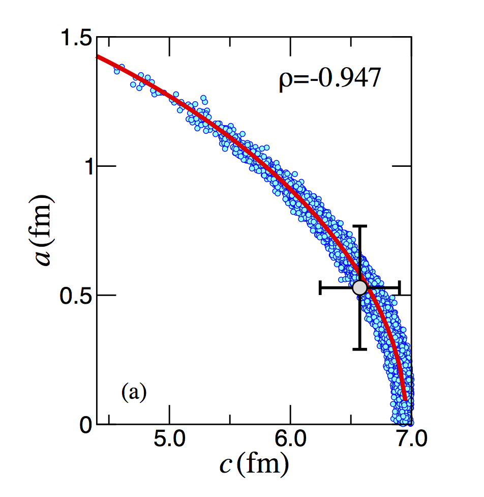
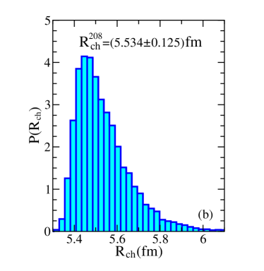
Figure 1: (color online) (a) Correlation plot between the half-density radius $c$ and the surface diffuseness $a$ that define the symmetrized Fermi function. The number of points represent the raw data obtained from the Monte-Carlo simulation. Also shown are the respective averages and standard deviations. The solid red line represents the functional form obtained from solving the equation $F_{\rm ch}(q_{1};a,c)\!=\!0.210$. (b) Probability distribution function for the charge radius of ²⁰⁸Pb obtained from the Monte-Carlo simulation.

With the definition of the posterior distribution now firmly in place, we proceed to generate the distribution of SFermi parameters using a standard Metropolis Monte-Carlo algorithm Metropolis et al. (1953). We underscore that the distribution of parameters is generated exclusively by the information that is presently known, namely, a single experimental measurement of the form factor that is encoded in the likelihood, and a set of theoretical biases that are embedded in the prior. The left-hand panel in Fig. 1 displays the correlation plot between the half-density radius $c$ and the surface diffuseness $a$ that define the SFermi distribution. As expected from just a single measurement, the model parameters are highly correlated. Indeed, the solid red line represents the functional relation implied by an ideal—i.e., error free and unbiased—single measurement of the form factor: ${F}_{\raisebox{-0.5pt}{\!\tiny ch}}({q}_{\raisebox{-1.5pt}{\tiny 1}};a,c)\!=\!0.210$. In turn, such a distribution of parameters generates the highly-asymmetric probability distribution function for the charge radius of ²⁰⁸Pb displayed on the right-hand panel of Fig. 1. For comparison, the experimental value is $R_{\rm ch}^{208}\!=\!5.5012(13)\,{\rm fm}$ Angeli and Marinova (2013).

As already alluded to and now clearly displayed in Fig. 2, there is a very large (indeed infinite!) number of pairs $(c,a)$ that pass through the single experimental point (indicated by the red circle). However, the plot is highly informative because it identifies the region of largest variability among the many models that satisfy the experimental constraint. This variability is quantified in terms of the relative variance in the model predictions (green solid line) which is maximized in the region around ${q}_{\raisebox{-1.5pt}{\tiny 2}}\!=\!0.8\,{\rm fm}^{-1}$. This situation is highly favorable because the momentum transfer is large enough for the parity-violating asymmetry to be “sizable” (as the asymmetry scales with $q^{2}$) but not overly large for the nuclear form factor to be highly suppressed.

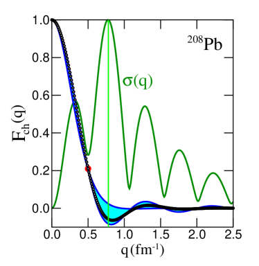
Figure 2: (color online) Variability in the charge form factor of ²⁰⁸Pb generated by the distribution of parameters displayed in Fig. 1. Also shown with the green solid line is the relative uncertainty in the model predictions as a function of the momentum transfer.

Having identified the second $q$-point, we are now ready to answer the central question posed in this manuscript: How accurately can we describe the form factor of ²⁰⁸Pb by measuring only two points? To answer this question we repeat the same procedure that we have just implemented but now with a likelihood function augmented by a second value of the charge form factor at the newly identified momentum transfer of ${q}_{\raisebox{-1.5pt}{\tiny 2}}\!=\!0.8\,{\rm fm}^{-1}$, namely, ${F}_{\raisebox{-0.5pt}{\!\tiny ch}}({q}_{\raisebox{-1.5pt}{\tiny 2}})\!=\!-0.0614$. For simplicity, we assume the same prior distribution and the same experimental error as before; that is, $\Delta F_{\rm exp}({q}_{\raisebox{-1.5pt}{\tiny 1}})\!=\!\Delta F_{\rm exp}({q}_{\raisebox{-1.5pt}{\tiny 2}})\!=\!0.005$.

The improvement in our knowledge of the underlying symmetrized Fermi function is readily apparent in Fig. 3. This figure is the analog of Fig. 1, although note the disparity in scales between the two figures. The distribution of parameters is displayed on the left-hand panel of Fig. 3 together with the 39% (in yellow) and 95% (in blue) confidence ellipsoids. Note that now the posterior distribution is constrained by two functional relations: ${F}_{\raisebox{-0.5pt}{\!\tiny ch}}({q}_{\raisebox{-1.5pt}{\tiny 1}};a,c)\!=\!0.210$ (solid red line) and ${F}_{\raisebox{-0.5pt}{\!\tiny ch}}({q}_{\raisebox{-1.5pt}{\tiny 2}};a,c)\!=\!-0.061$ (solid purple line) which together provide nearly “orthogonal” constraints that set stringent limits on both the half-density radius $c$ and the surface diffuseness $a$; see Table 2. Finally, the right-hand panel in Fig. 3 shows the probability distribution function for the charge radius of ²⁰⁸Pb [see Eq. (8)]; along with the best Gaussian fit. Thus, the theoretical prediction for the charge radius of ²⁰⁸Pb obtained from the knowledge of only two experimental points is $R_{\rm ch}^{208}\!=\!5.504(45)\,{\rm fm}$, which compares very favorably with the corresponding experimental value of $R_{\rm ch}^{208}\!=\!5.5012(13)\,{\rm fm}$ Angeli and Marinova (2013).

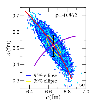
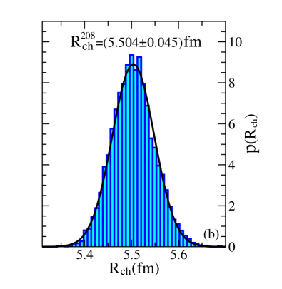
Figure 3: (color online) (a) Correlation plot between the half-density radius $c$ and the surface diffuseness $a$ that define the symmetrized Fermi function. The number of points represent the raw data obtained from the Monte-Carlo simulation. Also shown are the 39% and 95% confidence ellipses. The solid red and purple lines represents the functional form obtained from solving the equations: $F_{\rm ch}(q_{1};a,c)\!=\!0.210$ $F_{\rm ch}(q_{2};a,c)\!=\!-0.061$. (b) Probability distribution function for the charge radius of ²⁰⁸Pb obtained from the Monte-Carlo simulation. The black solid line represents a fit to a Gaussian probability distribution.

SFermi	Helm
$c=6.655\pm 0.081$	$R_{0}=6.785\pm 0.057$
$a=0.514\pm 0.066$	$\sigma=0.913\pm 0.116$
$R_{\rm ch}=5.504\pm 0.045$	$R_{\rm ch}=5.492\pm 0.041$

Table 2: Average values and corresponding theoretical uncertainties generated from the posterior distribution for a symmetrized Fermi and Helm form factors. Also shown are the predictions for the charge radius of ²⁰⁸Pb, which should be compared against the experimental value of $R_{\rm exp}^{208}\!=\!(5.5012\pm 0.0013)\,{\rm fm}$ Angeli and Marinova (2013). All quantities are given in fm.

Having calibrated the parameters of the symmetrized Fermi function using two experimental points and a fairly unconstrained prior distribution, we are now in a position to examine the overall agreement between the theoretical predictions and the experimental data for the entire charge form factor. This is shown in Fig. 4a using both linear and logarithmic scales. The two isolated red points represent the two experimental measurements that were used to calibrate the model parameters ($c$ and $a$). In turn, the dense collection of black points represents the full experimental form factor De Vries et al. (1987) that we aim to reproduce. Our theoretical predictions are displayed with a blue solid line together with the theoretical-uncertainty band shown in cyan. On a linear scale, it is difficult to discern the agreement (or lack-thereof) between theory and experiment. Moreover, on a linear scale it is also difficult to appreciate the diffractive oscillations modulated by an exponential envelope that are the hallmark of the nuclear form factor. Thus, we display on the inset in Fig. 4a the absolute value of the form factor using a logarithmic scale. The diffractive oscillations (controlled by $c$) and the exponential envelope (controlled by $a$) are now easily discernible. We observe a fairly good agreement between theory and experiment over several diffractive maxima up to momentum transfers well beyond the value of the second point (${q}_{\raisebox{-1.5pt}{\tiny 2}}\!=\!0.8\,{\rm fm}^{-1}$). However, at the largest momentum transfers displayed in the figure, i.e., $q\!\gtrsim\!2.5\,{\rm fm}^{-1}$, there is a clear deterioration in the model predictions. Finally, the associated charge density of ²⁰⁸Pb is displayed in Fig. 4b. Although it provides an excellent description of the experimental data at large distances as evinced in the inset, it fails to account for the experimental “dip” in the nuclear interior, which correlates with the deterioration of the theoretical predictions at large momentum transfers. Note that in contrast, accurately-calibrated mean-field models tend to overestimate the dip in the nuclear interior which is sensitive to shell effects Fattoyev et al. (2010); see Fig. 6.

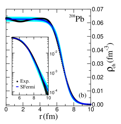
Figure 4: (color online) (a) Charge form factor and (b) the corresponding charge density of ²⁰⁸Pb. The two red points on the left-hand panel represent the sole input used in the calibration of the symmetrized Fermi function. The theoretical predictions are displayed by an uncertainty band (in cyan) and the experimental data is from Ref. De Vries et al. (1987).

For completeness, we display in Fig. 5 the form factor and corresponding spatial density of ²⁰⁸Pb—but now using the Helm representation. Here too the agreement with experiment is fairly good and underscores the fact that any two-parameter function that properly encapsulates the diffractive oscillations an the exponential falloff of the form factor is likely to provide an adequate description of the data, at least at low momentum transfers. Naturally, the great virtue of the symmetrized Fermi and Helm parameterizations is that both the spatial density and the form factor are known in closed analytic form. However, a distinct advantage of the former over the latter is that it displays an exponential rather than a Gaussian falloff at large distances.

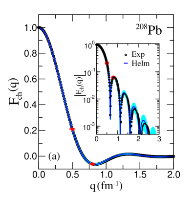
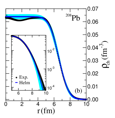
Figure 5: (color online) (a) Charge form factor and (b) the corresponding charge density of ²⁰⁸Pb. The two red points represent the sole input used in the calibration of the Helm function. The theoretical predictions are displayed by an uncertainty band (in cyan) and the experimental data is from Ref. De Vries et al. (1987).

As mentioned repeatedly earlier, the main goal of this manuscript is to assess using exclusively statistical methods and physical insights the impact of a second electroweak measurement of the weak form factor of ²⁰⁸Pb. In particular, we aim to quantify the experimental precision required in the determination of the weak-charge (or neutron) radius of ²⁰⁸Pb to have a strong impact on both nuclear structure and astrophysics. Using the charge form factor of ²⁰⁸Pb as a proxy, we found that by measuring two suitable points with relative small, yet attainable, errors, the charge radius of ²⁰⁸Pb could be reproduced accurately with a precision of about $0.04\,{\rm fm}$. It is therefore natural to ask how meaningful would a measurement of the weak-charge radius of ²⁰⁸Pb to this precision be on constraining the density dependence of the symmetry energy?

To elucidate this question we display in Table 3 predictions for several relevant quantities computed with a recent set of accurately calibrated relativistic mean field models. These models are constrained by the same isoscalar sector but differ in a single isovector assumption, namely, the choice of the neutron skin thickness of ²⁰⁸Pb Chen and Piekarewicz (2015). Although the set of models is relatively small, note that the theoretical spread in $R_{\rm wk}^{208}$ is nearly five times as large as the assumed $(0.04\,{\rm fm})$ experimental precision. Pictorially, the imprint of the isovector sector is illustrated in Fig. 6. Indeed, whereas the charge density remains practically unchanged, significant differences emerge in the weak-charge density, as the latter is dominated by the neutron distribution. Shown in the inset on a logarithmic scale are symmetrized Fermi and Helm fits to the RMF charge density that evinced the more realistic exponential falloff of the SFermi density. As a figure of merit, we can establish that if $R_{\rm wk}^{208}$ is relatively small, i.e., in the $R_{\rm wk}^{208}\!=\!(5.64\!-\!5.72)\,{\rm fm}$ range, or within the assumed $\pm 0.04\,{\rm fm}$ uncertainty, one could constrain the slope of the symmetry energy to about $15\,{\rm MeV}$ and the radius of a $1.4\,M_{\odot}$ neutron star to within $1.2\,{\rm km}$. Of course, these estimates are based on a very limited set of RMF models that suffer from their own limitations and theoretical biases. Yet, our conclusions appear consistent with other studies that incorporate a very large ensemble of reasonable nuclear energy density functionals Roca-Maza et al. (2011); Piekarewicz et al. (2012).

Model	$R_{\rm ch}^{208}$	$R_{\rm wk}^{208}$	$R_{\rm wk}^{208}\!-\!R_{\rm ch}^{208}$	$F_{\rm wk}^{\rm PREX}$	$L$	$R(1.4M_{\odot})$
RMF-012	5.504	5.636	0.132	0.239	48.254	12.400
RMF-016	5.499	5.667	0.168	0.234	50.961	12.839
RMF-022	5.496	5.722	0.226	0.226	63.524	13.609
RMF-028	5.495	5.790	0.295	0.216	112.644	14.234
RMF-032	5.489	5.822	0.333	0.212	125.626	14.718

Table 3: Predictions from a set of accurately calibrated relativistic mean-field models Chen and Piekarewicz (2015) for the charge radius, weak-charge radius, and their difference for ²⁰⁸Pb (all in fm). Also shown is the weak-charge form factor at the PREX momentum transfer, the slope of the symmetry energy $L$ (in MeV) and the radius of a $1.4\,M_{\odot}$ neutron star (in km). Some of these quantities may be compared against the following experimental values: $R_{\rm ch}^{208}\!=\!5.5012(13)\,{\rm fm}$ Angeli and Marinova (2013), $F_{\rm wk}^{\rm PREX}\!=\!0.204(28)$, and $R_{\rm wk}^{208}\!=\!5.826(181)\,{\rm fm}$ Horowitz et al. (2012).

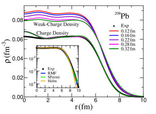
Figure 6: (color online) Charge and weak-charge density of ²⁰⁸Pb as predicted by a collection of accurately calibrated mean-field models. The labels indicate the predicted neutron-skin thickness of ²⁰⁸Pb. The inset displays the fastest Gaussian falloff of the Helm form factor relative to the exponential falloff of symmetrized Fermi function. The experimental data is from Ref. De Vries et al. (1987).

IV Conclusions

Almost 80 years ago and shortly after the discovery of the neutron by Chadwick, Bethe and Weizsäcker described the atomic nucleus as a two-component quantum drop with a constant interior density and a nearly universal surface. Since then, elastic electron scattering experiments have provided a detailed map of the charge distribution that validates the simple picture of Bethe and Weizsäcker. Indeed, to a large extent the nuclear charge density can be accurately described by only two parameters: a radius and a diffuseness. These two parameters leave their imprint in the characteristic diffractive oscillations modulated by an exponential falloff of the charge form factor. In this way, elastic electron scattering has provided the most accurate map of the distribution of charge in the nucleus.

Unfortunately, our picture of the corresponding weak-charge density is fairly crude. Whereas the charge density is dominated by the protons, the weak-charge density is dominated by the neutrons, as the weak neutral $Z^{0}$ boson couples preferentially to the neutrons. However, probing the neutron distribution is enormously challenging. Strongly interacting probes such as pions and protons couple strongly to neutrons but these reactions are plagued by hadronic uncertainties. Instead, parity-violating electron scattering is clean and model independent but the measured asymmetry is very small. Fortunately, in a pioneering measurement, the PREX collaboration used parity-violating electron scattering to extract the weak-charge form factor of ²⁰⁸Pb at a single value of the momentum transfer Abrahamyan et al. (2012).

In this manuscript we used standard statistical methods and physical insights to assess the impact of a second electroweak measurement of the weak-charge form factor of ²⁰⁸Pb. To do so, we introduced—or rather re-introduced Sprung and Martorell (1997)—the two-parameter symmetrized Fermi function, that is practically identical to the conventional Fermi function, but with far superior analytic properties. Indeed, the symmetrized Fermi function has a form factor that is known exactly in closed analytic form. By using such a parametrization, we estimated the accuracy and precision by which the root-mean-square radius of the distribution may be extracted from a single experimental measurement. Given that the symmetrized Fermi function—or any other realistic parametrization—requires the determination of two parameters, it is perhaps not surprising that we found a large number of combinations of parameters that satisfy the single experimental constraint and, thus, a resulting RMS radius that was neither accurate nor precise. So the natural follow-up task involved estimating the potential improvement in the determination of the RMS radius from a measurement of the form factor at a suitably chosen second point. To address this task we used the exquisitely known experimental charge form factor of ²⁰⁸Pb as a proxy for the weak charge form factor. To select the second point we examined the largest spread in the predictions of all the symmetrized Fermi models that satisfy the original (one point) constraint. Based on the largest variability, the optimal second point was identified near the first diffraction maximum (i.e., near the first maximum in $|F(q)|$ away from $q\!=\!0$). Incorporating this second point into the posterior probability density resulted in a significant improvement. First, we observed that the two measurements provide nearly “orthogonal” constraints that lift the original degeneracy among the parameters. Second, we obtained a RMS radius that is both accurate ($R_{\rm ch}^{208}\!=\!5.504\,{\rm fm}$) and precise ($\Delta R_{\rm ch}^{208}\!=\!0.045\,{\rm fm}$) as compared with the enormously precise experimental value of $R_{\rm exp}^{208}\!=\!5.5012(13)\,{\rm fm}$. Finally, when compared against the entire experimental charge form factor, the two-parameter symmetrized Fermi function provides an excellent description over several diffraction maxima.

So how accurately could one constrain the density dependence of the symmetry energy if the weak-charge radius of ²⁰⁸Pb could be measured with a precision of about $0.04\,{\rm fm}$? Based on a limited set of accurately calibrated RMF models, we estimated that a $\pm 0.04\,{\rm fm}$ determination of $R_{\rm wk}^{208}$ would translate into an overall constraint on the slope of the symmetry energy of about $15\,{\rm MeV}$. That is, if the symmetry energy is soft leading to a thin neutron skin, then $L$ was predicted to lie in the $L\!\approx\!(48\!-\!63)\,{\rm MeV}$ range. Although these RMF models are hindered by their own limitations and theoretical biases, more comprehensive studies using a large set of both non-relativistic and relativistic energy density functionals are consistent with these results. In fact, they often suggest even more stringent limits! While we recognize that achieving a $\pm 0.04\,{\rm fm}$ (or better) precision represents an enormous experimental challenge, the strong impact of a second measurement of the weak form factor of ²⁰⁸Pb on both nuclear and neutron-star structure may be worth the significant effort.