Electromagnetic Scattering for Time-Domain Maxwell’s Equations in an Unbounded Structure

Abstract.

The goal of this work is to study the electromagnetic scattering problem of time-domain Maxwell’s equations in an unbounded structure. An exact transparent boundary condition is developed to reformulate the scattering problem into an initial-boundary value problem in an infinite rectangular slab. The well-posedness and stability are established for the reduced problem. Our proof is based on the method of energy, the Lax–Milgram lemma, and the inversion theorem of the Laplace transform. Moreover, a priori estimates with explicit dependence on the time are achieved for the electric field by directly studying the time-domain Maxwell equations.

1. Introduction

Consider the propagation of an electromagnetic wave which is excited by electric current density and is scattered by infinite rough surfaces. An infinite rough surface is a non-local perturbation of an infinite plane surface such that the whole surface lies within a finite distance of the original plane. The goal of this paper is to examine the electromagnetic scattering problem of time-domain Maxwell’s equation in such an unbounded structure. The problem studied in this work falls into the class of rough surface scattering problems, which arise from various applications such as modeling acoustic and electromagnetic wave propagation over outdoor ground and sea surfaces, optical scattering from the surface of materials in near-field optics or nano-optics, detection of underwater mines, especially those buried in soft sediments. These problems are widely studied in the literature and various methods have been investigated [19, 21, 24, 27, 8, 9].

The infinite rough surfaces scattering problems are quite challenging due to unbounded domains. The usual Sommerfeld (for acoustic waves) or Silver–Müller (for electromagnetic waves) radiation condition is not valid any more [28, 1]. The Fredholm alternative theorem is not applicable due to the lack of compactness result. We refer to [2, 3, 4, 15, 13] for some mathematical studies on the two-dimensional Helmholtz equation. The rigorous mathematical analysis is very rare for the three-dimensional Maxwell equations. In [17], the electromagnetic scattering by unbounded rough surfaces was considered by assuming that the medium was lossy in the entire space. The well-posedness was established by a direct application of the Lax–Milgram theorem after showing that the sesquilinear form was coercive. In [11], the authors considered the electromagnetic scattering by an unbounded dielectric medium which was deposited on a perfectly electrically conducting plate. Based on the limiting absorption principle, the problem was shown to have a unique weak solution from a prior estimates. The magnetic permeability was assumed to be a constant and the electric current was assumed to be divergence free. The assumption was also restrictive for the dielectric permittivity. In [18], the generalized Lax–Milgram theorem was adopted to establish the well-posedness for the same problem as that in [11]. Although all the assumptions were relaxed, such as the magnetic permeability was allowed to be a variable function and the divergence free condition was removed for the electric current, the assumption was still quite restrictive for the dielectric permittivity. Despite the tremendous effort made so far, it is still unclear what the least restrictive conditions are for the dielectric permittivity and the magnetic permeability to assure the well-posedness of the time-harmonic Maxwell equations in unbounded structures. Ultimately, one wishes to answer the following question: Is the scattering problem in unbounded structures well-posed for the real and dielectric permittivity and magnetic permeability?

In this work, an initial attempt is made to study the time-domain electromagnetic scattering by infinite rough surfaces for the most difficult case of the time-harmonic counterpart: the dielectric permittivity and the magnetic permeability are assumed to be real and bounded measurable functions. An exact time-domain transparent boundary condition (TBC) is developed to reduce the scattering problem into an initial-boundary value problem in an infinite rectangular slab. To show the well-posedness, we split the reduced problem into two sub-problems: one has homogeneous initial conditions and another has a homogeneous boundary condition. Hence two auxiliary scattering problems need to be considered: one is the time-harmonic Maxwell equations with a complex wavenumber and another is the time-domain Maxwell equations with perfectly electrically conducting (PEC) boundary condition. Based on the stability results for the auxiliary problems, the reduced problem is shown to have a unique solution. Our proofs rely on the Laplace transform, the Lax–Milgram theorem, and the Parseval identity between the frequency domain and the time-domain. Moreover, a priori estimates, featuring an explicit dependence on the time and a minimum regularity requirement of the initial conditions and the source term, are established for the electric field by studying directly the time-domain Maxwell equations.

The time-domain scattering problems have recently attracted considerable attention due to their capability of capturing wide-band signals and modeling more general material and nonlinearity [5, 12, 14, 20, 26], which motivates us to tune our focus from seeking the best possible conditions for those physical parameters to the time-domain problem. Comparing with the time-harmonic problems, the time-domain problems are less studied due to the additional challenge of the temporal dependence. The analysis can be found in [25, 6] for the time-domain acoustic and electromagnetic obstacle scattering problems. We refer to [16] for the analysis of the time-dependent electromagnetic scattering from a three-dimensional open cavity. Numerical solutions can be found in [10, 23] for the time-dependent wave scattering by periodic structures.

The paper is organized as follows. In section 2, the model problem is introduced and reduced equivalently into an initial-boundary value problem by using a TBC. Some regularity properties of the trace operator are presented. In section 3, two auxiliary problems of Maxwell’s equations are discussed to pave the way for the analysis of the main result in section 4. Section 4 is devoted to the well-posedness and stability of the reduced time-domain Maxwell equations and a priori estimates of the solution. The paper is concluded with some general remarks in section 5.

2. Problem formulation

In this section, we introduce the model problem and present an exact time-domain transparent boundary condition to reduce the scattering problem into an initial-boundary value problem in an infinite rectangular slab.

2.1. A model problem

Let us first introduce the problem geometry which is shown in Figure 1. Let $S_{j},j=1,2$ be Lipschitz continuous surfaces which are embedded in the infinite rectangular slab

$$\Omega=\{\boldsymbol{x}=(x,y,z)^{\top}\in\mathbb{R}^{3}:h_{2}<z<h_{1}\},$$

where $h_{j}$ are constants. Denote by $\Gamma_{j}=\{\boldsymbol{x}:z=h_{j}\}$ the two plane surfaces which enclose $\Omega$. Let $\Omega_{1}=\{\boldsymbol{x}:z>h_{1}\}$ and $\Omega_{2}=\{\boldsymbol{x}:z<h_{2}\}$. The medium is assumed to be homogeneous in $\Omega_{j}$, but it is allowed to be inhomogeneous in $\Omega$.

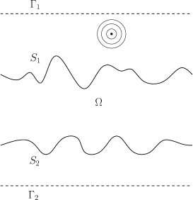
Figure 1. Problem geometry of the electromagnetic scattering by an unbounded structure

The electromagnetic field is governed by the time-domain Maxwell equations in $\mathbb{R}^{3}$ for $t>0$:

$$\nabla\times\boldsymbol{E}(\boldsymbol{x},t)+\mu\partial_{t}\boldsymbol{H}(\boldsymbol{x},t)=0,\quad\nabla\times\boldsymbol{H}(\boldsymbol{x},t)-\varepsilon\partial_{t}\boldsymbol{E}(\boldsymbol{x},t)=\boldsymbol{J}(\boldsymbol{x},t),$$ (2.1)

where $\boldsymbol{E}$ is the electric field, $\boldsymbol{H}$ is the magnetic field, $\boldsymbol{J}$ is the electric current density which is assumed to be compactly supported in $\Omega$, the material parameters $\varepsilon$ and $\mu$ are the dielectric permittivity and the magnetic permeability, respectively. We assume that $\varepsilon\in L^{\infty}(\mathbb{R}^{3})$ and $\mu\in L^{\infty}(\mathbb{R}^{3})$ satisfy

$$0<\varepsilon_{\min}\leq\varepsilon\leq\varepsilon_{\max}<\infty,\quad 0<\mu_{\min}\leq\mu\leq\mu_{\max}<\infty,$$

where $\varepsilon_{\min},\varepsilon_{\max},\mu_{\min},\mu_{\max}$ are constants. Since the medium is homogeneous in $\Omega_{j}$, there exist constants $\varepsilon_{j}$ and $\mu_{j}$ such that

$$\varepsilon(\boldsymbol{x})=\varepsilon_{j},\quad\mu(\boldsymbol{x})=\mu_{j}\quad{\rm in}~{}\Omega_{j}.$$

The system is constrained by the initial conditions:

$$\boldsymbol{E}|_{t=0}=\boldsymbol{E}_{0},\quad\boldsymbol{H}|_{t=0}=\boldsymbol{H}_{0}\quad{\rm in}~{}\mathbb{R}^{3},$$ (2.2)

where $\boldsymbol{E}_{0}$ and $\boldsymbol{H}_{0}$ are also assumed to be compactly supported in $\Omega$. Due to the unbounded structure of the medium, it is no longer valid to impose the usual Silver–Müler radiation condition. We employ the following radiation condition: the electromagnetic fields $(\boldsymbol{E},\boldsymbol{H})$ consist of bounded outgoing waves in $\Omega_{j}$.

2.2. Functional spaces

We introduce some Sobolev space notation. For $u\in L^{2}(\Gamma_{j})$, we denote by $\hat{u}$ the Fourier transform of $u$, i.e.,

$$\hat{u}(\boldsymbol{\xi},h_{j})=\frac{1}{2\pi}\int_{\mathbb{R}^{2}}u(\boldsymbol{\rho},h_{j})e^{-{\rm i}\boldsymbol{\rho}\cdot\boldsymbol{\xi}}{\rm d}\boldsymbol{\rho},$$

where $\boldsymbol{\xi}=(\xi_{1},\xi_{2})^{\top}\in\mathbb{R}^{2}$ and $\boldsymbol{\rho}=(x,y)^{\top}\in\mathbb{R}^{2}.$ Denote by $C_{\boldsymbol{\rho}}^{\infty}$ the linear space of infinitely differentiable functions with compact support with respect to the variable $\boldsymbol{\rho}$ on $\Omega.$ Let $L^{2}(\Omega)$ be the space of complex square integrable functions on $\Omega$. It follows from the Parseval identity that we have

$$\|u\|^{2}_{L^{2}(\Omega)}=\int_{h_{2}}^{h_{1}}\int_{\mathbb{R}^{2}}|u(\boldsymbol{\rho},z)|^{2}{\rm d}\boldsymbol{\rho}{\rm d}z=\int_{h_{2}}^{h_{1}}\int_{\mathbb{R}^{2}}|\hat{u}(\boldsymbol{\xi},z)|^{2}{\rm d}\boldsymbol{\xi}{\rm d}z.$$

Introduce the functional spaces

$$\boldsymbol{H}({\rm curl},\Omega) =\{\boldsymbol{u}\in\boldsymbol{L}^{2}(\Omega),\nabla\times\boldsymbol{u}\in\boldsymbol{L}^{2}(\Omega)\},$$

$$\boldsymbol{H}_{0}({\rm curl},\Omega) =\{\boldsymbol{u}\in\boldsymbol{H}({\rm curl},\Omega),\boldsymbol{u}\times\boldsymbol{n}_{j}=0~{}\text{on}~{}\Gamma_{j}\},$$

which are Sobolev spaces with the norm

$$\|\boldsymbol{u}\|_{\boldsymbol{H}({\rm curl},\Omega)}=\Big{(}\|\boldsymbol{u}\|^{2}_{\boldsymbol{L}^{2}(\Omega)}+\|\nabla\times\boldsymbol{u}\|^{2}_{\boldsymbol{L}^{2}(\Omega)}\Big{)}^{1/2}.$$

Given $\boldsymbol{u}=(u_{1}(\boldsymbol{\rho},z),u_{2}(\boldsymbol{\rho},z),u_{3}(\boldsymbol{\rho},z))^{\top}\in\boldsymbol{H}({\rm curl},\Omega),$ it has the inverse Fourier transform:

$$\boldsymbol{u}(\boldsymbol{\rho},z)=\frac{1}{2\pi}\int_{\mathbb{R}^{2}}\big{(}\hat{u}_{1}(\boldsymbol{\xi},z),\hat{u}_{2}(\boldsymbol{\xi},z),\hat{u}_{3}(\boldsymbol{\xi},z)\big{)}^{\top}e^{{\rm i}\boldsymbol{\rho}\cdot\boldsymbol{\xi}}{\rm d}\boldsymbol{\xi}.$$

The norm in $\boldsymbol{H}({\rm curl},\Omega)$ can be defined via Fourier coefficients:

$$\|\boldsymbol{u}\|^{2}_{\boldsymbol{H}({\rm curl},\Omega)}=\int_{h_{2}}^{h_{1}}\int_{\mathbb{R}^{2}} \big{[}|\hat{u}_{1}(\boldsymbol{\xi},z)|^{2}+|\hat{u}_{2}(\boldsymbol{\xi},z)|^{2}+|\hat{u}_{3}(\boldsymbol{\xi},z)|^{2}+|{\rm i}\xi_{2}\hat{u}_{3}(\boldsymbol{\xi},z)-\hat{u}_{2}^{\prime}(\boldsymbol{\xi},z)|^{2}$$

$$+|\hat{u}_{1}^{\prime}(\boldsymbol{\xi},z)-{\rm i}\xi_{1}\hat{u}_{3}(\boldsymbol{\xi},z)|^{2}+|\xi_{1}\hat{u}_{2}(\boldsymbol{\xi},z)-\xi_{2}\hat{u}_{1}(\boldsymbol{\xi},z)|^{2}\big{]}{\rm d}\boldsymbol{\xi}{\rm d}z,$$

where $\hat{u}_{j}^{\prime}(\boldsymbol{\xi},z)=\partial_{z}\hat{u}_{j}(\boldsymbol{\xi},z).$

Lemma 2.1.

$C_{\boldsymbol{\rho}}^{\infty}(\Omega)^{3}$ is dense in $\boldsymbol{H}({\rm curl},\Omega).$

Proof.

Noting that $C_{0}^{\infty}(\mathbb{R}^{3})^{3}$ is dense in $\boldsymbol{H}({\rm curl},\mathbb{R}^{3})$ , we have $C_{0}^{\infty}(\mathbb{R}^{3})^{3}|_{\Omega}$ is dense in $\boldsymbol{H}({\rm curl},\mathbb{R}^{3})|_{\Omega}.$ From the Sobolev extension theorem, $\boldsymbol{H}({\rm curl},\mathbb{R}^{3})|_{\Omega}=\boldsymbol{H}({\rm curl},\Omega).$ Therefore $C_{\boldsymbol{\rho}}^{\infty}(\Omega)^{3}\supseteq C_{0}^{\infty}(\mathbb{R}^{3})^{3}|_{\Omega}$ is dense in $\boldsymbol{H}({\rm curl},\Omega).$ ∎

This density lemma is useful to deal with the infinite domain $\Omega$. We may prove the results only on $C_{\boldsymbol{\rho}}^{\infty}(\Omega)^{3}$ and then extend them by limiting argument to more general functions such as those in $\boldsymbol{H}(\rm curl,\Omega)$. Consequently, the boundary integrals only on $\Gamma_{j}$ need to be considered when formulating the variational problems in $\Omega$.

For any vector field $\boldsymbol{u}=(u_{1},u_{2},u_{3})^{\top}$, denote by

$$\boldsymbol{u}_{\Gamma_{j}}=\boldsymbol{n}_{j}\times(\boldsymbol{u}\times\boldsymbol{n}_{j})=(u_{1}(x,y,h_{j}),u_{2}(x,y,h_{j}),0)^{\top}$$

the tangential component on $\Gamma_{j}$, where $\boldsymbol{n}_{1}=(0,0,1)^{\top}$ and $\boldsymbol{n}_{2}=(0,0,-1)^{\top}$ are the unit outward normal vectors on $\Gamma_{1}$ and $\Gamma_{2}$, respectively. For any smooth vector $\boldsymbol{u}=(u_{1},u_{2},u_{3})^{\top}$ defined on $\Gamma_{j}$, let ${\rm div}_{\Gamma_{j}}\boldsymbol{u}=\partial_{x}u_{1}+\partial_{y}u_{2}$ and ${\rm curl}_{\Gamma_{j}}\boldsymbol{u}=\partial_{x}u_{2}-\partial_{y}u_{1}$ be the surface divergence and surface scalar curl of the field $\boldsymbol{u}$. For a smooth scalar function $u$, denote by $\nabla_{\Gamma_{j}}u=(\partial_{x}u,\partial_{y}u,0)^{\top}$ the surface gradient on $\Gamma_{j}$.

Let $H^{-1/2}(\Gamma_{j})$ be the completion of $L^{2}(\Gamma_{j})$ in the norm

$$\|u\|_{H^{-1/2}(\Gamma_{j})}=\Big{(}\int_{\mathbb{R}^{2}}(1+|\boldsymbol{\xi}|^{2})^{-1/2}|\hat{u}|^{2}{\rm d}\boldsymbol{\xi}\Big{)}^{1/2}.$$

Introduce two tangential functional spaces:

$$\boldsymbol{H}^{-1/2}({\rm curl},\Gamma_{j}) =\{\boldsymbol{u}\in H^{-1/2}(\Gamma_{j})^{3}:u_{3}=0,~{}{\rm curl}_{\Gamma_{j}}\boldsymbol{u}\in H^{-1/2}(\Gamma_{j})\},$$

$$\boldsymbol{H}^{-1/2}({\rm div},\Gamma_{j}) =\{\boldsymbol{u}\in H^{-1/2}(\Gamma_{j})^{3}:u_{3}=0,~{}{\rm div}_{\Gamma_{j}}\boldsymbol{u}\in H^{-1/2}(\Gamma_{j})\},$$

which are equipped with the norms:

$$\|\boldsymbol{u}\|_{\boldsymbol{H}^{-1/2}({\rm curl},~{}\Gamma_{j})} =\Big{(}\int_{\mathbb{R}^{2}}(1+|\boldsymbol{\xi}|^{2})\big{[}|\hat{u}_{1}|^{2}+|\hat{u}_{2}|^{2}+|\xi_{1}\hat{u}_{2}-\xi_{2}\hat{u}_{1}|^{2}\big{]}{\rm d}\boldsymbol{\xi}\Big{)}^{1/2},$$

$$\|\boldsymbol{u}\|_{\boldsymbol{H}^{-1/2}({\rm div},~{}\Gamma_{j})} =\Big{(}\int_{\mathbb{R}^{2}}(1+|\boldsymbol{\xi}|^{2})\big{[}|\hat{u}_{1}|^{2}+|\hat{u}_{2}|^{2}+|\xi_{1}\hat{u}_{1}+\xi_{2}\hat{u}_{2}|^{2}\big{]}{\rm d}\boldsymbol{\xi}\Big{)}^{1/2}.$$

The following two lemmas are concerned with the duality between the spaces $\boldsymbol{H}^{-1/2}({\rm div},\Gamma_{j})$ and $\boldsymbol{H}^{1/2}({\rm curl},\Gamma_{j})$ and the trace regularity in $\boldsymbol{H}({\rm curl},\Omega)$. The proofs can be found in [17, Lemma 2.3, Lemma 2.4].

Lemma 2.2.

The spaces $\boldsymbol{H}^{-1/2}({\rm div},\Gamma_{j})$ and $\boldsymbol{H}^{1/2}({\rm curl},\Gamma_{j})$ are mutually adjoint with respect to the scalar product in $L^{2}(\Gamma_{j})^{3}$ defined by

$$\langle\boldsymbol{u},\boldsymbol{v}\rangle_{\Gamma_{j}}=\int_{\Gamma_{j}}\boldsymbol{u}\cdot\bar{\boldsymbol{v}}{\rm d}\gamma_{j}=\int_{\mathbb{R}^{2}}(\hat{u}_{1}\bar{\hat{v}}_{1}+\hat{u}_{2}\bar{\hat{v}}_{2}){\rm d}\boldsymbol{\xi}.$$ (2.3)

Lemma 2.3.

Let $C=\max\{\sqrt{1+(h_{1}-h_{2})^{-1}},\sqrt{2}\}$. We have the estimate

$$\|\boldsymbol{u}\|_{\boldsymbol{H}^{-1/2}({\rm curl},~{}\Gamma_{j})}\leq C\|\boldsymbol{u}\|_{\boldsymbol{H}({\rm curl},\Omega)},\quad\forall~{}\boldsymbol{u}\in\boldsymbol{H}({\rm curl},\Omega).$$

Next we introduce some properties of the Laplace transform. Let $s=s_{1}+{\rm i}s_{2}$ with $s_{1}>0,s_{2}\in\mathbb{R}$. Define by $\breve{\boldsymbol{u}}(s)$ the Laplace transform of $\boldsymbol{u}(t)$, i.e.,

$$\breve{\boldsymbol{u}}(s)=\mathscr{L}(\boldsymbol{u})(s)=\int_{0}^{\infty}e^{-st}\boldsymbol{u}(t){\rm d}t.$$

Using the integration by parts yields

$$\int_{0}^{t}\boldsymbol{u}(\tau){\rm d}\tau=\mathscr{L}^{-1}(s^{-1}\breve{\boldsymbol{u}}(s)),$$ (2.4)

where $\mathscr{L}^{-1}$ is the inverse Laplace transform. It is also easy to verify that

$$\boldsymbol{u}(t)=\mathscr{F}^{-1}\big{(}e^{s_{1}t}\mathscr{L}(\boldsymbol{u})(s_{1}+s_{2})\big{)},$$ (2.5)

where $\mathscr{F}^{-1}$ denotes the inverse Fourier transform with respect to $s_{2}$. Recall the Plancherel or the Parseval identity for the Laplace transform (cf. [7, (2.46)]):

$$\frac{1}{2\pi}\int_{-\infty}^{\infty}\breve{\boldsymbol{u}}(s)\breve{\boldsymbol{v}}(s){\rm d}s_{2}=\int_{0}^{\infty}e^{-2s_{1}t}{\boldsymbol{u}}(t){\boldsymbol{v}}(t){\rm d}t,\quad\forall~{}s_{1}>\lambda,$$ (2.6)

where $\breve{\boldsymbol{u}}=\mathscr{L}(\boldsymbol{u}),\breve{\boldsymbol{v}}=\mathscr{L}(\boldsymbol{v})$ and $\lambda$ is abscissa of convergence for the Laplace transform of $\boldsymbol{u}$ and $\boldsymbol{v}.$

The following lemma ([22, Theorem 43.1]) is an analogue of the Paley–Wiener–Schwarz theorem for the Fourier transform of distributions with compact support in the case of the Laplace transform.

Lemma 2.4.

Let $\breve{\boldsymbol{h}}(s)$ be a holomorphic function in the half-plane $s_{1}>\sigma_{0}$ and be valued in the Banach space $\mathbb{E}$. The following two statements are equivalent:

1. There is a distribution $\breve{\boldsymbol{h}}\in\mathcal{D}_{+}^{\prime}(\mathbb{E})$ whose Laplace transform is equal to $\breve{\boldsymbol{h}}(s)$;

2. There is a real $\sigma_{1}$ with $\sigma_{0}\leq\sigma_{1}<\infty$ and an integer $m\geq 0$ such that for all complex numbers $s$ with ${\rm Re}s=s_{1}>\sigma_{1},$ it holds that $\|\breve{\boldsymbol{h}}(s)\|_{\mathbb{E}}\lesssim(1+|s|)^{m}$,

where $\mathcal{D}^{\prime}_{+}(\mathbb{E})$ is the space of distributions on the real line which vanishes identically in the open negative half line.

2.3. Transparent boundary condition

We introduce an exact time-domain TBC to formulate the scattering problem into the following initial-boundary value problem:

$$\begin{cases}\nabla\times\boldsymbol{E}+\mu\partial_{t}\boldsymbol{H}=0,\quad\nabla\times\boldsymbol{H}-\varepsilon\partial_{t}\boldsymbol{E}=\boldsymbol{J}\quad&{\rm in}~{}\Omega,~{}t>0,\\ \boldsymbol{E}|_{t=0}=\boldsymbol{E}_{0},\quad\boldsymbol{H}|_{t=0}=\boldsymbol{H}_{0}\quad&{\rm in}~{}\Omega,\\ \mathscr{T}_{j}[\boldsymbol{E}_{\Gamma_{j}}]=\boldsymbol{H}\times n_{j}\quad&{\rm on}~{}\Gamma_{j},~{}t>0,\end{cases}$$ (2.7)

where $\boldsymbol{E}_{\Gamma_{j}}$ is the tangential component of $\boldsymbol{E}$ on $\Gamma_{j}$ and $\mathscr{T}_{j}$ is the time-domain electric-to-magnetic capacity operator.

In what follows, we shall derive the formulation of the operators $\mathscr{T}_{j}$ and show some of their properties. Since the derivation of $\mathscr{T}_{1}$ and $\mathscr{T}_{2}$ is analogous, we will only show the details for $\mathscr{T}_{1}$ and state the corresponding result on $\mathscr{T}_{2}$ without derivation.

Notice that $\boldsymbol{J}$ is supported in $\Omega$ and $\varepsilon=\varepsilon_{1},\mu=\mu_{1}$ in $\Omega_{1}$, the system of Maxwell equations (2.1) reduce to

$$\nabla\times\boldsymbol{E}+\mu_{1}\partial_{t}\boldsymbol{H}=0,\quad\nabla\times\boldsymbol{H}-\varepsilon_{1}\partial_{t}\boldsymbol{E}=0\quad{\rm in}~{}\Omega_{1},~{}t>0.$$ (2.8)

Let $\breve{\boldsymbol{E}}(\boldsymbol{x},s)$ and $\breve{\boldsymbol{H}}(\boldsymbol{x},s)$ be the Laplace transform of $\boldsymbol{E}(\boldsymbol{x},t)$ and $\boldsymbol{H}(\boldsymbol{x},t)$. Recall that

$$\mathscr{L}(\partial_{t}\boldsymbol{E})=s\breve{\boldsymbol{E}}-{\boldsymbol{E}}_{0},\quad\mathscr{L}(\partial_{t}\boldsymbol{H})=s\breve{\boldsymbol{H}}-\boldsymbol{H}_{0}.$$

Taking the Laplace transform of (2.8), and noting that $\boldsymbol{E}_{0}$ and $\boldsymbol{H}_{0}$ are supported in $\Omega,$ we obtain the Maxwell equations in the $s$-domain:

$$\nabla\times\breve{\boldsymbol{E}}+\mu_{1}s\breve{\boldsymbol{H}}=0,\quad\nabla\times\breve{\boldsymbol{H}}-\varepsilon_{1}s\breve{\boldsymbol{E}}=0\quad{\rm in}~{}\Omega_{1},~{}s_{1}>0,~{}s_{2}\in\mathbb{R}.$$ (2.9)

Let $\breve{\boldsymbol{E}}=(\breve{E}_{1},\breve{E}_{2},\breve{E}_{3})^{\top}$ and $\breve{\boldsymbol{H}}=(\breve{H}_{1},\breve{H}_{2},\breve{H}_{3})^{\top}$. Denote by $\breve{\boldsymbol{E}}_{\Gamma_{1}}=(\breve{E}_{1}(\boldsymbol{\rho},h_{1}),\breve{E}_{2}(\boldsymbol{\rho},h_{1}),0)^{\top}$ the tangential component of the electric field on $\Gamma_{1}$. Let $\breve{\boldsymbol{H}}\times\boldsymbol{n}_{1}=(\breve{H}_{2}(\boldsymbol{\rho},h_{1}),-\breve{H}_{1}(\boldsymbol{\rho},h_{1}),0)^{\top}$ be the tangential trace of the magnetic field on $\Gamma_{1}.$ It follows from (2.9) that

$$\breve{H}_{2}(\boldsymbol{\rho},h_{1}) =\frac{1}{\mu_{1}s}[\partial_{x}\breve{E}_{3}(\boldsymbol{\rho},h_{1})-\partial_{z}\breve{E}_{1}(\boldsymbol{\rho},h_{1})],$$

$$-\breve{H}_{1}(\boldsymbol{\rho},h_{1}) =\frac{1}{\mu_{1}s}[\partial_{y}\breve{E}_{3}(\boldsymbol{\rho},h_{1})-\partial_{z}\breve{E}_{2}(\boldsymbol{\rho},h_{1})].$$

Taking the Fourier transform of the above equations with respect to $\boldsymbol{\rho}$ gives

$$\hat{\breve{H}}_{2}(\boldsymbol{\xi},h_{1}) =\dfrac{1}{\mu_{1}s}[{\rm i}\xi_{1}\hat{\breve{E}}_{3}(\boldsymbol{\xi},h_{1})-\partial_{z}\hat{\breve{E}}_{1}(\boldsymbol{\xi},h_{1})],$$ (2.10a)

$$-\hat{\breve{H}}_{1}(\boldsymbol{\xi},h_{1}) =\dfrac{1}{\mu_{1}s}[{\rm i}\xi_{2}\hat{\breve{E}}_{3}(\boldsymbol{\xi},h_{1})-\partial_{z}\hat{\breve{E}}_{2}(\boldsymbol{\xi},h_{1})].$$ (2.10b)

Observe that the medium is homogeneous in $\Omega_{1}$, which gives $\nabla\cdot\breve{\boldsymbol{E}}=0$ in $\Omega_{1}.$ Eliminating the magnetic field from (2.9) and using the divergence free condition in $\Omega_{1}$, we obtain the Helmholtz equation for the components of the electric field:

$$\begin{cases}\Delta\breve{E}_{j}(\boldsymbol{\rho},z)-\varepsilon_{1}\mu_{1}s^{2}\breve{E}_{j}(\boldsymbol{\rho},z)=0\quad&{\rm in}~{}\Omega_{1},\\ \breve{E}_{j}(\boldsymbol{\rho},z)=\breve{E}_{j}(\boldsymbol{\rho},h_{1})\quad&{\rm on}~{}\Gamma_{1}.\end{cases}$$

Taking the Fourier transform with respect to $\boldsymbol{\rho}$ of the above equations yields

$$\begin{cases}\partial_{z}^{2}\hat{\breve{E}}_{j}-(\varepsilon_{1}\mu_{1}s^{2}+|\boldsymbol{\xi}|^{2})\hat{\breve{E}}_{j}=0,\quad&z>h_{1},\\ \hat{\breve{E}}_{j}=\hat{\breve{E}}_{j}(\boldsymbol{\xi},h_{1}),\quad&z=h_{1}.\end{cases}$$

Solving the above equations and using the bounded outgoing condition, we obtain the solution:

$$\hat{\breve{E}}_{j}(\boldsymbol{\xi},z)=\hat{\breve{E}}_{j}(\boldsymbol{\xi},h_{1})e^{-\beta_{1}(\boldsymbol{\xi})(z-h_{1})},\quad z>h_{1},$$ (2.11)

where

$$\beta_{1}(\boldsymbol{\xi})=(\varepsilon_{1}\mu_{1}s^{2}+|\boldsymbol{\xi}|^{2})^{1/2},\quad{\rm Re}\beta_{1}(\boldsymbol{\xi})>0.$$

Taking the derivative of (2.11) with respect to $z$ and evaluating it at $z=h_{1}$, we get

$$\partial_{z}\hat{\breve{E}}_{j}(\boldsymbol{\xi},h_{1})=-\beta_{1}(\boldsymbol{\xi})\hat{\breve{E}}_{j}(\boldsymbol{\xi},h_{1}).$$

Noting that $\nabla\cdot\breve{\boldsymbol{E}}=\partial_{x}\breve{E}_{1}+\partial_{y}\breve{E}_{2}+\partial_{z}\breve{E}_{3}=0$ in $\Omega_{1}$ and $\beta_{1}(\boldsymbol{\xi})\neq 0$ for all $\boldsymbol{\xi},$ we deduce that

$$\hat{\breve{E}}_{3}(\boldsymbol{\xi},h_{1})=\frac{-1}{\beta_{1}(\boldsymbol{\xi})}\partial_{z}\hat{\breve{E}}_{3}(\boldsymbol{\xi},h_{1})=\frac{{\rm i}}{\beta_{1}(\boldsymbol{\xi})}[\xi_{1}\hat{\breve{E}}_{1}(\boldsymbol{\xi},h_{1})+\xi_{2}\hat{\breve{E}}_{2}(\boldsymbol{\xi},h_{1})].$$

Therefore, we have from (2.10) that

$$\hat{\breve{H}}_{2}(\boldsymbol{\xi},h_{1}) =\frac{1}{\mu_{1}s}\left[\frac{-\xi_{1}}{\beta_{1}(\boldsymbol{\xi})}\bigl{(}\xi_{1}\hat{\breve{E}}_{1}(\boldsymbol{\xi},h_{1})+\xi_{2}\hat{\breve{E}}_{2}(\boldsymbol{\xi},h_{1})\bigr{)}+\beta_{1}(\boldsymbol{\xi})\hat{\breve{E}}_{1}(\boldsymbol{\xi},h_{1})\right],$$

$$-\hat{\breve{H}}_{1}(\boldsymbol{\xi},h_{1}) =\frac{1}{\mu_{1}s}\left[\frac{-\xi_{2}}{\beta_{1}(\boldsymbol{\xi})}\bigl{(}\xi_{1}\hat{\breve{E}}_{1}(\boldsymbol{\xi},h_{1})+\xi_{2}\hat{\breve{E}}_{2}(\boldsymbol{\xi},h_{1})\bigr{)}+\beta_{1}(\boldsymbol{\xi})\hat{\breve{E}}_{2}(\boldsymbol{\xi},h_{1})\right],$$

or equivalently,

$$\hat{\breve{H}}_{2}(\boldsymbol{\xi},h_{1}) =\frac{1}{\mu_{1}s\beta_{1}(\boldsymbol{\xi})}\left[\varepsilon_{1}\mu_{1}s^{2}\hat{\breve{E}}_{1}(\boldsymbol{\xi},h_{1})+\xi_{2}\bigl{(}\xi_{2}\hat{\breve{E}}_{1}(\boldsymbol{\xi},h_{1})-\xi_{1}\hat{\breve{E}}_{2}(\boldsymbol{\xi},h_{1})\bigr{)}\right],$$

$$-\hat{\breve{H}}_{1}(\boldsymbol{\xi},h_{1}) =\frac{1}{\mu_{1}s\beta_{1}(\boldsymbol{\xi})}\left[\varepsilon_{1}\mu_{1}s^{2}\hat{\breve{E}}_{2}(\boldsymbol{\xi},h_{1})+\xi_{1}\bigl{(}\xi_{1}\hat{\breve{E}}_{2}(\boldsymbol{\xi},h_{1})-\xi_{2}\hat{\breve{E}}_{1}(\boldsymbol{\xi},h_{1})\bigr{)}\right].$$

For any tangential vector $\boldsymbol{u}=(u_{1},u_{2},0)^{\top}$ on $\Gamma_{1}$, define the capacity operator $\mathscr{B}_{1}$:

$$\mathscr{B}_{1}[\boldsymbol{u}]=(v_{1},v_{2},0)^{\top},$$

where

$$\hat{v}_{1} =\frac{1}{\mu_{1}s}\big{[}-\frac{\xi_{1}}{\beta_{1}}(\xi_{1}\hat{u}_{1}+\xi_{2}\hat{u}_{2})+\beta_{1}\hat{u}_{1}\big{]},$$ (2.12a)

$$\hat{v}_{2} =\frac{1}{\mu_{1}s}\big{[}-\frac{\xi_{2}}{\beta_{1}}(\xi_{1}\hat{u}_{1}+\xi_{2}\hat{u}_{2})+\beta_{1}\hat{u}_{2}\big{]},$$ (2.12b)

or equivalently,

$$\hat{v}_{1} =\frac{1}{\mu_{1}s\beta_{1}}\big{[}\varepsilon_{1}\mu_{1}s^{2}\hat{u}_{1}+\xi_{2}(\xi_{2}\hat{u}_{1}-\xi_{1}\hat{u}_{2})\big{]},$$ (2.13a)

$$\hat{v}_{2} =\frac{1}{\mu_{1}s\beta_{1}}\big{[}\varepsilon_{1}\mu_{1}s^{2}\hat{u}_{2}+\xi_{1}(\xi_{1}\hat{u}_{2}-\xi_{2}\hat{u}_{1})\big{]}.$$ (2.13b)

Similarly, for any tangential vector $\boldsymbol{u}=(u_{1},u_{2},0)$ on $\Gamma_{2}$, define the capacity operator $\mathscr{B}_{2}$:

$$\mathscr{B}_{2}[\boldsymbol{u}]=(v_{1},v_{2},0)^{\top},$$

where

$$\hat{v}_{1} =\frac{1}{\mu_{2}s}\big{[}\beta_{2}\hat{u}_{1}-\frac{\xi_{1}}{\beta_{2}}(\xi_{1}\hat{u}_{1}+\xi_{2}\hat{u}_{2})\big{]},$$ (2.14a)

$$\hat{v}_{2} =\frac{1}{\mu_{2}s}\big{[}\beta_{2}\hat{u}_{2}-\frac{\xi_{2}}{\beta_{2}}(\xi_{1}\hat{u}_{1}+\xi_{2}\hat{u}_{2})\big{]},$$ (2.14b)

or equivalently,

$$\hat{v}_{1} =\frac{1}{\mu_{2}s\beta_{2}}\big{[}\varepsilon_{2}\mu_{2}s^{2}\hat{u}_{1}+\xi_{2}(\xi_{2}\hat{u}_{1}-\xi_{1}\hat{u}_{2})\big{]},$$ (2.15a)

$$\hat{v}_{2} =\frac{1}{\mu_{2}s\beta_{2}}\big{[}\varepsilon_{2}\mu_{2}s^{2}\hat{u}_{2}+\xi_{1}(\xi_{1}\hat{u}_{2}-\xi_{2}\hat{u}_{1})\big{]},$$ (2.15b)

where

$$\beta_{2}(\boldsymbol{\xi})=(\varepsilon_{2}\mu_{2}s^{2}+|\boldsymbol{\xi}|^{2})^{1/2},\quad{\rm Re}\beta_{2}(\boldsymbol{\xi})>0.$$

For any vector field $\breve{\boldsymbol{E}}\in\boldsymbol{H}({\rm curl},\Omega)$, it follows from Lemma 2.3 that its tangential component $\breve{\boldsymbol{E}}_{\Gamma_{j}}\in\boldsymbol{H}^{-1/2}({\rm curl},\Gamma_{j}).$ Using the capacity operators, we may propose the following TBC in the $s$-domain:

$$\mathscr{B}_{j}[\breve{\boldsymbol{E}}_{\Gamma_{j}}]=\breve{\boldsymbol{H}}\times\boldsymbol{n}_{j}\quad{\rm on}~{}\Gamma_{j},$$ (2.16)

where the capacity operator $\mathscr{B}_{j}$ maps the tangential component of the electric field to the tangential trace of the magnetic field. Taking the inverse Laplace transform of (2.16) yields the TBC in the time-domain:

$$\mathscr{T}_{j}[\boldsymbol{E}_{\Gamma_{j}}]=\boldsymbol{H}\times\boldsymbol{n}_{j},$$

where $\mathscr{T}_{j}=\mathscr{L}^{-1}\circ\mathscr{B}_{j}\circ\mathscr{L}$. Equivalently, we may eliminate the magnetic field and obtain an alternative TBC for the electric field in the $s$-domain:

$$\mu_{j}^{-1}s^{-1}(\nabla\times\breve{\boldsymbol{E}})\times\boldsymbol{n}_{j}+\mathscr{B}_{j}[\breve{\boldsymbol{E}}_{\Gamma_{j}}]=0\quad{\rm on}~{}\Gamma_{j}.$$ (2.17)

Correspondingly, by taking the inverse Laplace transform of (2.17), we may derive an alternative TBC for the electric field in the time-domain:

$$\mu_{j}^{-1}(\nabla\times\boldsymbol{E})\times\boldsymbol{n}_{j}+\mathscr{C}_{j}[\boldsymbol{E}_{\Gamma_{j}}]=0\quad{\rm on}\quad\Gamma_{j},$$ (2.18)

where $\mathscr{C}_{j}=\mathscr{L}^{-1}\circ s\mathscr{B}_{j}\circ\mathscr{L}.$

Lemma 2.5.

The capacity operator $\mathscr{B}_{j}:\boldsymbol{H}^{-1/2}({\rm curl},\Gamma_{j})\rightarrow\boldsymbol{H}^{-1/2}({\rm div},\Gamma_{j})$ is continuous.

Proof.

For any $\boldsymbol{u}=(u_{1},u_{2},0)^{\top},\boldsymbol{w}=(w_{1},w_{2},0)^{\top}\in\boldsymbol{H}^{-1/2}({\rm curl},\Omega),$ let $\mathscr{B}_{j}\boldsymbol{u}=(v_{1},v_{2},0)^{\top}.$ It follows from the definitions (2.3), (2.13), and (2.15) that

$$\langle\mathscr{B}_{j}\boldsymbol{u},\boldsymbol{w}\rangle_{\Gamma_{j}} =\int_{\mathbb{R}^{2}}(\hat{v}_{1}\bar{\hat{w}}_{1}+\hat{v}_{2}\bar{\hat{w}}_{2}){\rm d}\boldsymbol{\xi}$$

$$=\int_{\mathbb{R}^{2}}\frac{1}{\mu_{j}s\beta_{j}}\big{[}\varepsilon_{j}\mu_{j}s^{2}(\hat{u}_{1}\bar{\hat{w}}_{1}+\hat{u}_{2}\bar{\hat{w}}_{2})+(\xi_{1}\hat{u}_{2}-\xi_{2}\hat{u}_{1})(\xi_{1}\bar{\hat{w}}_{2}-\xi_{2}\bar{\hat{w}}_{1})\big{]}{\rm d}\boldsymbol{\xi}$$

$$=\int_{\mathbb{R}^{2}}\frac{(1+|\boldsymbol{\xi}|^{2})^{1/2}}{\mu_{j}s\beta_{j}}(1+|\boldsymbol{\xi}|^{2})^{-1/2}\big{[}\varepsilon_{j}\mu_{j}s^{2}(\hat{u}_{1}\bar{\hat{w}}_{1}+\hat{u}_{2}\bar{\hat{w}}_{2})+(\xi_{1}\hat{u}_{2}-\xi_{2}\hat{u}_{1})(\xi_{1}\bar{\hat{w}}_{2}-\xi_{2}\bar{\hat{w}}_{1})\big{]}{\rm d}\boldsymbol{\xi}.$$

To prove the lemma, it is required to estimate

$$\frac{(1+|\boldsymbol{\xi}|^{2})^{1/2}}{|\beta_{j}|}.$$

Let

$$\varepsilon_{j}\mu_{j}s^{2}=a_{j}+{\rm i}b_{j},$$

where

$$a_{j}=\varepsilon_{j}\mu_{j}(s_{1}^{2}-s_{2}^{2}),\quad b_{j}=2\varepsilon_{j}\mu_{j}s_{1}s_{2}.$$

Denote

$$\beta_{j}^{2}=\varepsilon_{j}\mu_{j}s^{2}+|\boldsymbol{\xi}|^{2}=\phi_{j}+{\rm i}b_{j},$$

where

$$\phi_{j}={\rm Re}(\varepsilon_{j}\mu_{j}s^{2})+|\boldsymbol{\xi}|^{2}=a_{j}+|\boldsymbol{\xi}|^{2}.$$

A simple calculation gives

$$\frac{(1+|\boldsymbol{\xi}|^{2})^{1/2}}{|\beta_{j}|}=\left[\frac{(1+\phi_{j}-a_{j})^{2}}{\phi_{j}^{2}+b_{j}^{2}}\right]^{1/4}.$$

Let

$$F_{j}(t)=\frac{(1+t-a_{j})^{2}}{t^{2}+b_{j}^{2}},$$

which gives

$$F_{j}^{\prime}(t)=\frac{2(1+t-a_{j})(b_{j}^{2}-t(1-a_{j}))}{(t^{2}+b_{j}^{2})^{2}}.$$

We consider three cases:

• $1-a_{j}>0$. It can be verified that the function $F_{j}(t)$ increases for $a_{j}\leq t\leq K_{j}=b_{j}^{2}/(1-a_{j})$ and decreases for $t>K_{j}$. Hence $F_{j}(t)$ reaches its maximum at $t=K_{j}$, i.e.,

  $$\frac{(1+\phi_{j}-a_{j})^{2}}{\phi_{j}^{2}+b_{j}^{2}}=F_{j}(\phi_{j})\leq F_{j}(K_{j})=\frac{(1-a_{j})^{2}+b_{j}^{2}}{b_{j}^{2}}.$$

• $1-a_{j}=0$. It is easy to verify

  $$F_{j}(t)=\frac{t^{2}}{t^{2}+b_{j}^{2}}\leq 1.$$

  which yields that

  $$F_{j}(\phi_{j})\leq 1\leq\frac{(1-a_{j})^{2}+b_{j}^{2}}{b_{j}^{2}}.$$

• $1-a_{j}<0$. It follows from $K_{j}\leq a_{j}$ that $F_{j}(t)$ increases for $t\leq K_{j}$ and decreases for $K_{j}<t$. Since $\phi_{j}=a_{j}+|\boldsymbol{\xi}|^{2}\geq a_{j}$, we have

  $$F_{j}(\phi_{j})\leq F_{j}(a_{j})=\frac{1}{a_{j}^{2}+b_{j}^{2}}\leq F_{j}(K_{j})=\frac{(1-a_{j})^{2}+b_{j}^{2}}{b_{j}^{2}}.$$

Combing the above estimates yields

$$|\langle\mathscr{B}_{j}\boldsymbol{u},\boldsymbol{w}\rangle_{\Gamma_{j}}|\leq C_{j}\|\boldsymbol{u}\|_{\boldsymbol{H}^{-1/2}({\rm curl},~{}\Gamma_{j})}\|\boldsymbol{w}\|_{\boldsymbol{H}^{-1/2}({\rm curl},~{}\Gamma_{j})}$$

where

$$C_{j}=\frac{1}{\mu_{j}s_{1}}\left[\frac{(1-a_{j})^{2}+b_{j}^{2}}{b_{j}^{2}}\right]^{1/4}\times\max\{(a_{j}^{2}+b_{j}^{2})^{1/2},~{}1\}.$$

Following from Lemma 2.2, we have

$$\|\mathscr{B}_{j}\boldsymbol{u}\|_{\boldsymbol{H}^{-1/2}({\rm div},~{}\Gamma_{j})}\leq C\sup\limits_{\boldsymbol{w}\in\boldsymbol{H}^{-1/2}({\rm curl},~{}\Gamma_{j})}\frac{|\langle\mathscr{B}_{j}\boldsymbol{u},\boldsymbol{w}\rangle_{\Gamma_{j}}|}{\|\boldsymbol{w}\|_{\boldsymbol{H}^{-1/2}({\rm curl},~{}\Gamma_{j})}}\leq CC_{j}\|\boldsymbol{u}\|_{\boldsymbol{H}^{-1/2}({\rm curl},~{}\Gamma_{j})},$$

which completes the proof. ∎

Lemma 2.6.

We have

$${\rm Re}\langle\mathscr{B}_{j}\boldsymbol{u},\boldsymbol{u}\rangle_{\Gamma_{j}}\geq 0,\quad\forall~{}\boldsymbol{u}\in\boldsymbol{H}^{-1/2}({\rm curl},\Gamma_{j}).$$

Proof.

By definitions (2.3), (2.12), and (2.14), we obtain

$$\langle\mathscr{B}_{j}\boldsymbol{u},\boldsymbol{u}\rangle_{\Gamma_{j}} =\frac{1}{\mu_{j}s}\int_{\mathbb{R}^{2}}\big{[}\beta_{j}(|\hat{u}_{1}|^{2}+|\hat{u}_{2}|^{2})-\frac{1}{\beta_{j}}|\xi_{1}\hat{u}_{1}+\xi_{2}\hat{u}_{2}|^{2}\big{]}{\rm d}\boldsymbol{\xi}$$

$$=\frac{1}{\mu_{j}|s|^{2}}\int_{\mathbb{R}^{2}}\big{[}\bar{s}\beta_{j}(|\hat{u}_{1}|^{2}+|\hat{u}_{2}|^{2})-\frac{\bar{s}\bar{\beta_{j}}}{|\beta_{j}|^{2}}|\xi_{1}\hat{u}_{1}+\xi_{2}\hat{u}_{2}|^{2}\big{]}{\rm d}\boldsymbol{\xi}.$$

Let $\beta_{j}=m_{j}+{\rm i}n_{j}$ with $m_{j}>0.$ Taking the real part of the above equation gives

$${\rm Re}\langle\mathscr{B}_{j}\boldsymbol{u},\boldsymbol{u}\rangle_{\Gamma_{j}}=\frac{1}{\mu_{j}|s|^{2}}\int_{\mathbb{R}^{2}}\big{[} (m_{j}s_{1}+n_{j}s_{2})(|\hat{u}_{1}|^{2}+|\hat{u}_{2}|^{2})$$

$$- \frac{(m_{j}s_{1}-n_{j}s_{2})}{m_{j}^{2}+n_{j}^{2}}|\xi_{1}\hat{u}_{1}+\xi_{2}\hat{u}_{2}|^{2}\big{]}{\rm d}\boldsymbol{\xi}.$$

Recalling $\beta_{j}^{2}=\varepsilon_{j}\mu_{j}s^{2}+|\boldsymbol{\xi}|^{2},$ we have

$$m_{j}^{2}-n_{j}^{2} =\varepsilon_{j}\mu_{j}(s_{1}^{2}-s_{2}^{2})+|\boldsymbol{\xi}|^{2},$$ (2.19)

$$m_{j}n_{j} =\varepsilon_{j}\mu_{j}s_{1}s_{2}.$$ (2.20)

Using (2.20), we get

$$m_{j}s_{1}+n_{j}s_{2}=\frac{s_{1}}{m_{j}}[m_{j}^{2}+\varepsilon_{j}\mu_{j}s_{2}^{2}],\quad m_{j}s_{1}-n_{j}s_{2}=\frac{s_{1}}{m_{j}}[m_{j}^{2}-\varepsilon_{j}\mu_{j}s_{2}^{2}].$$

If $m_{j}^{2}-\varepsilon_{j}\mu_{j}s_{2}^{2}\leq 0$, we obtain

$${\rm Re}\langle\mathscr{B}_{j}\boldsymbol{u},\boldsymbol{u}\rangle_{\Gamma_{j}}=\frac{1}{\mu_{j}|s|^{2}}\int_{\mathbb{R}^{2}} \frac{s_{1}}{m_{j}}\big{[}(m_{j}^{2}+\varepsilon_{j}\mu_{j}s_{2}^{2})(|\hat{u}_{1}|^{2}+|\hat{u}_{2}|^{2})$$

$$- \frac{(m_{j}^{2}-\varepsilon_{j}\mu_{j}s_{2}^{2})}{m_{j}^{2}+n_{j}^{2}}|\xi_{1}\hat{u}_{1}+\xi_{2}\hat{u}_{2}|^{2}\big{]}{\rm d}\boldsymbol{\xi}\geq 0.$$

If $m_{j}^{2}-\varepsilon_{j}\mu_{j}s_{2}^{2}>0$, we have from the Cauchy–Schwarz inequality that

$$\frac{(m_{j}^{2}-\varepsilon_{j}\mu_{j}s_{2}^{2})}{m_{j}^{2}+n_{j}^{2}}|\xi_{1}\hat{u}_{1}+\xi_{2}\hat{u}_{2}|^{2}\leq\frac{(m_{j}^{2}-\varepsilon_{j}\mu_{j}s_{2}^{2})}{m_{j}^{2}+n_{j}^{2}}|\boldsymbol{\xi}|^{2}(|\hat{u}_{1}|^{2}+|\hat{u}_{2}|^{2}),$$

which gives

$${\rm Re}\langle\mathscr{B}_{j}\boldsymbol{u},\boldsymbol{u}\rangle_{\Gamma_{j}}\geq\frac{1}{\mu_{j}|s|^{2}}\int_{\mathbb{R}^{2}} \frac{s_{1}}{m_{j}}\Bigl{[}(m_{j}^{2}+\varepsilon_{j}\mu_{j}s_{2}^{2})$$

$$- \frac{(m_{j}^{2}-\varepsilon_{j}\mu_{j}s_{2}^{2})}{m_{j}^{2}+n_{j}^{2}}|\boldsymbol{\xi}|^{2}\Bigr{]}(|\hat{u}_{1}|^{2}+|\hat{u}_{2}|^{2}){\rm d}\boldsymbol{\xi}.$$ (2.21)

Substituting (2.19) into (2.3) yields

$${\rm Re}\langle\mathscr{B}_{j}\boldsymbol{u},\boldsymbol{u}\rangle_{\Gamma_{j}}\geq\frac{1}{\mu_{j}|s|^{2}}\int_{\mathbb{R}^{2}} \frac{s_{1}}{m_{j}(m_{j}^{2}+n_{j}^{2})}\bigl{[}(m_{j}^{2}+\varepsilon_{j}\mu_{j}s_{2}^{2})(n_{j}^{2}+\varepsilon_{j}\mu_{j}s_{2}^{2})$$

$$+ (m_{j}^{2}-\varepsilon_{j}\mu_{j}s_{2}^{2})(n_{j}^{2}+\varepsilon_{j}\mu_{j}s_{1}^{2})\bigr{]}(|\hat{u}_{1}|^{2}+|\hat{u}_{2}|^{2}){\rm d}\boldsymbol{\xi}\geq 0,$$

which completes the proof. ∎

In the forthcoming sections, we shall use the method of energy to prove the well-posedness and stability of the reduced problem (2.7). We point out that the method has also been adopted in [16] for solving the time-dependent electromagnetic scattering problem from an open cavity.

3. Two auxiliary problems

In this section, we present the energy estimates for two auxiliary problems, one is the time-harmonic Maxwell equations with a complex wavenumber and another is the time-domain Maxwell equations with a perfectly electrically conducting (PEC) boundary condition. These estimates will be used for the proof of the main results for the time-domain Maxwell equations (2.7).

3.1. Time-harmonic Maxwell’s equations with a complex wavenumber

We shall study the variational formulation for a time-harmonic Maxwell equations with a complex wavenumber, which is a frequency version of the initial-boundary value problem of the Maxwell equations under the Laplace transform.

Consider the auxiliary boundary value problem:

$$\left\{\begin{array}[]{ll}\nabla\times\big{(}(s\mu)^{-1}\nabla\times\boldsymbol{u}\big{)}+s\varepsilon\boldsymbol{u}=\boldsymbol{j}&\text{in}~{}\Omega,\\ \mu_{j}^{-1}s^{-1}(\nabla\times{\boldsymbol{u}})\times\boldsymbol{n}_{j}+\mathscr{B}_{j}[{\boldsymbol{u}}_{\Gamma_{j}}]=0&\text{on}~{}\Gamma_{j},\end{array}\right.$$ (3.1)

where $s=s_{1}+{\rm i}s_{2}$ with $s_{1}>0,s_{2}\in\mathbb{R}$ and $\boldsymbol{j}$ is assumed to be compactly supported in $\Omega.$

Multiplying the complex conjugate of a test function $\boldsymbol{v}\in\boldsymbol{H}({\rm curl},\Omega),$ integrating over $\Omega$, and using integration by parts, we arrive at the variational formulation of (3.1): Find $\boldsymbol{u}\in\boldsymbol{H}({\rm curl},\Omega)$ such that

$$a_{\rm TH}(\boldsymbol{u},\boldsymbol{v})=\int_{\Omega}\boldsymbol{j}\cdot\bar{\boldsymbol{v}}{\rm d}\boldsymbol{x},\quad\forall~{}\boldsymbol{v}\in\boldsymbol{H}({\rm curl},\Omega),$$ (3.2)

where the sesquilinear form

$$a_{\rm TH}(\boldsymbol{u},\boldsymbol{v})=\int_{\Omega}(s\mu)^{-1}(\nabla\times\boldsymbol{u})\cdot(\nabla\times\bar{\boldsymbol{v}}){\rm d}\boldsymbol{x}+\int_{\Omega}s\varepsilon\boldsymbol{u}\cdot\bar{\boldsymbol{v}}{\rm d}\boldsymbol{x}+\sum\limits_{j=1}^{2}\langle\mathscr{B}_{j}[\boldsymbol{u}_{\Gamma_{j}}],\boldsymbol{v}_{\Gamma_{j}}\rangle_{\Gamma_{j}}.$$ (3.3)

Theorem 3.1.

The variational problem (3.2) has a unique solution $\boldsymbol{u}\in\boldsymbol{H}({\rm curl},\Omega)$ which satisfies

$$\|\nabla\times\boldsymbol{u}\|_{\boldsymbol{L}^{2}(\Omega)}+\|s\boldsymbol{u}\|_{\boldsymbol{L}^{2}(\Omega)}\lesssim s_{1}^{-1}\|s\boldsymbol{j}\|_{\boldsymbol{L}^{2}(\Omega)}.$$

Proof.

It suffices to show the coercivity of the sesquilinear form of $a_{\rm TH}$ since the continuity follows directly from the Cauchy–Schwarz inequality, Lemma 2.5, and Lemma 2.3.

Letting $\boldsymbol{v}=\boldsymbol{u}$, we have from (3.3) that

$$a_{\rm TH}(\boldsymbol{u},\boldsymbol{u})=\int_{\Omega}(s\mu)^{-1}|\nabla\times\boldsymbol{u}|^{2}{\rm d}\boldsymbol{x}+\int_{\Omega}s\varepsilon|\boldsymbol{u}|^{2}{\rm d}\boldsymbol{x}+\sum\limits_{j=1}^{2}\langle\mathscr{B}_{j}[\boldsymbol{u}_{\Gamma_{j}}],\boldsymbol{u}_{\Gamma_{j}}\rangle_{\Gamma_{j}}.$$ (3.4)

Taking the real part of (3.4) and using Lemma 2.6, we get

$${\rm Re}a_{\rm TH}(\boldsymbol{u},\boldsymbol{u})\geq\frac{s_{1}}{|s|^{2}}\big{(}\|\nabla\times\boldsymbol{u}\|^{2}_{\boldsymbol{L}^{2}(\Omega)}+\|s\boldsymbol{u}\|^{2}_{\boldsymbol{L}^{2}(\Omega)}\big{)}.$$ (3.5)

It follows from the Lax–Milgram lemma that the variational problem (3.2) has a unique solution $\boldsymbol{u}\in\boldsymbol{H}({\rm curl},\Omega)$. Moreover, we have from (3.2) that

$$|a_{\rm TH}(\boldsymbol{u},\boldsymbol{u})|\leq|s|^{-1}\|\boldsymbol{j}\|_{\boldsymbol{L}^{2}(\Omega)}\|s\boldsymbol{u}\|_{\boldsymbol{L}^{2}(\Omega)}.$$ (3.6)

Combing (3.5)–(3.6) leads to

$$\|\nabla\times\boldsymbol{u}\|^{2}_{\boldsymbol{L}^{2}(\Omega)}+\|s\boldsymbol{u}\|^{2}_{\boldsymbol{L}^{2}(\Omega)}\lesssim s_{1}^{-1}\|s\boldsymbol{j}\|_{\boldsymbol{L}^{2}(\Omega)}\|s\boldsymbol{u}\|_{\boldsymbol{L}^{2}(\Omega)},$$

which completes the proof after applying the Cauchy–Schwarz inequality. ∎

3.2. Time-domain Maxwell’s equations with PEC condition

Consider the initial-boundary value problem for the time-domain Maxwell equations with the PEC boundary condition:

$$\begin{cases}\nabla\times\boldsymbol{U}+\mu\partial_{t}\boldsymbol{V}=0,\quad\nabla\times\boldsymbol{V}-\varepsilon\partial_{t}\boldsymbol{U}=0\quad&\text{in}~{}\Omega,~{}t>0,\\ \boldsymbol{U}\times\boldsymbol{n}_{j}=0\quad&\text{on}~{}\Gamma_{j},~{}t>0,\\ \boldsymbol{U}|_{t=0}=\boldsymbol{E}_{0},\quad\boldsymbol{V}|_{t=0}=\boldsymbol{H}_{0}\quad&\text{in}~{}\Omega,\end{cases}$$ (3.7)

where $\boldsymbol{E}_{0},\boldsymbol{H}_{0}$ are assumed to be compactly supported in $\Omega$.

Let $\breve{\boldsymbol{U}}=\mathscr{L}(\boldsymbol{U})$ and $\breve{\boldsymbol{V}}=\mathscr{L}(\boldsymbol{V}).$ Taking the Laplace transform of (3.7) and eliminating $\breve{\boldsymbol{V}}$, we obtain the boundary value problem:

$$\begin{cases}\nabla\times\big{(}(s\mu)^{-1}\nabla\times\breve{\boldsymbol{U}}\big{)}+s\varepsilon\breve{\boldsymbol{U}}=\breve{\boldsymbol{j}}\quad&\text{in}~{}\Omega,\\ \breve{\boldsymbol{U}}\times\boldsymbol{n}_{j}=0\quad&\text{on}~{}\Gamma_{j},\end{cases}$$ (3.8)

where $\breve{\boldsymbol{j}}=\varepsilon\boldsymbol{E}_{0}+s^{-1}\nabla\times\boldsymbol{H}_{0}$. The variational formulation for (3.8) is to find $\breve{\boldsymbol{U}}\in\boldsymbol{H}_{0}({\rm curl,\Omega})$ such that

$$a_{\rm TD}(\breve{\boldsymbol{U}},\boldsymbol{v})=\int_{\Omega}\breve{\boldsymbol{j}}\cdot\bar{\boldsymbol{v}}{\rm d}\boldsymbol{x},\quad\forall~{}\boldsymbol{v}\in\boldsymbol{H}_{0}({\rm curl},\Omega),$$ (3.9)

where the sesquilinear from

$$a_{\rm TD}(\breve{\boldsymbol{U}},\boldsymbol{v})=\int_{\Omega}(s\mu)^{-1}(\nabla\times\breve{\boldsymbol{U}})\cdot(\nabla\times\bar{\boldsymbol{v}}){\rm d}\boldsymbol{x}+\int_{\Omega}s\varepsilon\breve{\boldsymbol{U}}\cdot\bar{\boldsymbol{v}}{\rm d}\boldsymbol{x}.$$

Following the same proof as that in Theorem 3.1, we may obtain the well-posedness of the variation problem (3.9) and its stability estimate.

Lemma 3.2.

The variational problem (3.8) has a unique solution $\breve{\boldsymbol{U}}\in\boldsymbol{H}_{0}({\rm curl},\Omega)$ which satisfies

$$\|\nabla\times\breve{\boldsymbol{U}}\|_{\boldsymbol{L}^{2}(\Omega)}+\|s\breve{\boldsymbol{U}}\|_{\boldsymbol{L}^{2}(\Omega)}\lesssim s_{1}^{-1}\|s\boldsymbol{E}_{0}\|_{\boldsymbol{L}^{2}(\Omega)}+s_{1}^{-1}\|\nabla\times\boldsymbol{H}_{0}\|_{\boldsymbol{L}^{2}(\Omega)}.$$

Theorem 3.3.

The auxiliary problem (3.7) has a unique solution $(\boldsymbol{U},\boldsymbol{V})$, which satisfies the stability estimates:

$$\|\boldsymbol{U}\|_{\boldsymbol{L}^{2}(\Omega)}+\|\boldsymbol{V}\|_{\boldsymbol{L}^{2}(\Omega)} \lesssim\|\boldsymbol{E}_{0}\|_{\boldsymbol{L}^{2}(\Omega)}+\|\boldsymbol{H}_{0}\|_{\boldsymbol{L}^{2}(\Omega)},$$

$$\|\partial_{t}\boldsymbol{U}\|_{\boldsymbol{L}^{2}(\Omega)}+\|\partial_{t}\boldsymbol{V}\|_{\boldsymbol{L}^{2}(\Omega)} \lesssim\|\nabla\times\boldsymbol{E}_{0}\|_{\boldsymbol{L}^{2}(\Omega)}+\|\nabla\times\boldsymbol{H}_{0}\|_{\boldsymbol{L}^{2}(\Omega)},$$

$$\|\partial^{2}_{t}\boldsymbol{U}\|_{\boldsymbol{L}^{2}(\Omega)}+\|\partial^{2}_{t}\boldsymbol{V}\|_{\boldsymbol{L}^{2}(\Omega)} \lesssim\|\nabla\times(\nabla\times\boldsymbol{E}_{0})\|_{\boldsymbol{L}^{2}(\Omega)}+\|\nabla\times(\nabla\times\boldsymbol{H}_{0})\|_{\boldsymbol{L}^{2}(\Omega)}.$$

Proof.

Let $\breve{\boldsymbol{U}}=\mathscr{L}(\boldsymbol{U})$ and $\breve{\boldsymbol{V}}=\mathscr{L}(\boldsymbol{V})$. Taking the Laplace transform of (3.7) and using the initial condition lead to

$$\left\{\begin{array}[]{ll}\nabla\times\breve{\boldsymbol{U}}+s\mu\breve{\boldsymbol{V}}=\mu\boldsymbol{H}_{0},\quad\nabla\times\breve{\boldsymbol{V}}-s\varepsilon\breve{\boldsymbol{U}}=-\varepsilon\boldsymbol{E}_{0}&\text{in}~{}\Omega,\\ \breve{\boldsymbol{U}}\times\boldsymbol{n}_{j}=0&\text{on}~{}\Gamma_{j}.\end{array}\right.$$ (3.10)

It follows from Lemma 3.2 that

$$\|\nabla\times\breve{\boldsymbol{U}}\|_{\boldsymbol{L}^{2}(\Omega)}+\|s\breve{\boldsymbol{U}}\|_{\boldsymbol{L}^{2}(\Omega)}\lesssim s_{1}^{-1}\|s\boldsymbol{E}_{0}\|_{\boldsymbol{L}^{2}(\Omega)}+s_{1}^{-1}\|\nabla\times\boldsymbol{H}_{0}\|_{\boldsymbol{L}^{2}(\Omega)}.$$

Combing the above inequality and (3.10) gives

$$\|-s\mu\breve{\boldsymbol{V}}+\mu\boldsymbol{H}_{0}\|_{\boldsymbol{L}^{2}(\Omega)}+\|\varepsilon^{-1}\nabla\times\breve{\boldsymbol{V}}+\boldsymbol{E}_{0}\|\lesssim s_{1}^{-1}\|s\boldsymbol{E}_{0}\|_{\boldsymbol{L}^{2}(\Omega)}+s_{1}^{-1}\|\nabla\times\boldsymbol{H}_{0}\|_{\boldsymbol{L}^{2}(\Omega)},$$

which shows that

$$\|\nabla\times{\breve{\boldsymbol{V}}}\|_{L^{2}(\Omega)}+\|s\breve{\boldsymbol{V}}\|_{\boldsymbol{L}^{2}(\Omega)}\lesssim(1+s_{1}^{-1}|s|)\|\boldsymbol{E}_{0}\|_{\boldsymbol{L}^{2}(\Omega)}+\|\boldsymbol{H}_{0}\|_{\boldsymbol{L}^{2}(\Omega)}+s_{1}^{-1}\|\nabla\times\boldsymbol{H}_{0}\|_{\boldsymbol{L}^{2}(\Omega)}.$$

It follows from [22, Lemma 44.1] that $\breve{\boldsymbol{U}}$ and $\breve{\boldsymbol{V}}$ are holomorphic functions of $s$ on the half plane $s_{1}>\bar{\gamma}>0,$ where $\bar{\gamma}$ is any positive constant. Hence we have from Lemma 2.4 that the inverse Laplace transform of $\breve{\boldsymbol{U}}$ and $\breve{\boldsymbol{V}}$ exist and they are supported in $[0,\infty).$

Next we prove the stability by the energy function method. Define the energy function

$$e_{1}(t)=\|\varepsilon^{1/2}\boldsymbol{U}(\cdot,t)\|^{2}_{\boldsymbol{L}^{2}(\Omega)}+\|\mu^{1/2}\boldsymbol{V}(\cdot,t)\|^{2}_{\boldsymbol{L}^{2}(\Omega)}.$$

Using (3.7) and integration by parts, we obtain

$$e_{1}(t)-e_{1}(0) =\int_{0}^{t}e_{1}^{\prime}(\tau){\rm d}\tau=2{\rm Re}\int_{0}^{t}\int_{\Omega}\big{(}\varepsilon\partial_{t}\boldsymbol{U}\cdot\bar{\boldsymbol{U}}+\mu\partial_{t}\boldsymbol{V}\cdot\bar{\boldsymbol{V}}\big{)}{\rm d}\boldsymbol{x}{\rm d}\tau$$

$$=2{\rm Re}\int_{0}^{t}\int_{\Omega}(\nabla\times\boldsymbol{V})\cdot\bar{\boldsymbol{U}}-(\nabla\times{\boldsymbol{U}})\cdot\bar{\boldsymbol{V}}{\rm d}\boldsymbol{x}{\rm d}\tau$$

$$=2{\rm Re}\int_{0}^{t}\int_{\Omega}\big{[}(\nabla\times{\boldsymbol{V}})\cdot\bar{\boldsymbol{U}}-(\nabla\times\bar{\boldsymbol{V}})\cdot{\boldsymbol{U}}\big{]}{\rm d}\boldsymbol{x}{\rm d}\tau-2{\rm Re}\int_{0}^{t}\sum\limits_{j=1}^{2}\langle\boldsymbol{U}\times\boldsymbol{n}_{j},{\boldsymbol{V}}\rangle_{\Gamma_{j}}{\rm d}\tau$$

$$=0.$$

Hence we have

$$\|\varepsilon^{1/2}\boldsymbol{U}(\cdot,t)\|^{2}_{\boldsymbol{L}^{2}}+\|\mu^{1/2}\boldsymbol{V}(\cdot,t)\|^{2}_{\boldsymbol{L}^{2}(\Omega)}=\|\varepsilon^{1/2}\boldsymbol{E}_{0}\|^{2}_{\boldsymbol{L}^{2}}+\|\mu^{1/2}\boldsymbol{H}_{0}\|^{2}_{\boldsymbol{L}^{2}(\Omega)},$$

which implies

$$\|\boldsymbol{U}\|_{\boldsymbol{L}^{2}(\Omega)}+\|\boldsymbol{V}\|_{\boldsymbol{L}^{2}(\Omega)}\lesssim\|\boldsymbol{E}_{0}\|_{L^{2}(\Omega)}+\|\boldsymbol{H}_{0}\|_{\boldsymbol{L}^{2}(\Omega)}.$$

Taking the first and second partial derivative of (3.7) with respect to $t$ yields

$$\left\{\begin{array}[]{ll}\nabla\times\partial_{t}\boldsymbol{U}+\mu\partial_{t}^{2}\boldsymbol{V}=0,\quad\nabla\times\partial_{t}\boldsymbol{V}-\varepsilon\partial_{t}^{2}\boldsymbol{U}=0&\text{in}~{}\Omega,~{}t>0,\\ \partial_{t}\boldsymbol{U}\times\boldsymbol{n}_{j}=0&\text{on}~{}\Gamma_{j},~{}t>0,\\ \partial_{t}\boldsymbol{U}|_{t=0}=\varepsilon^{-1}(\nabla\times\boldsymbol{H}_{0}),\quad\partial_{t}\boldsymbol{V}|_{t=0}=-\mu^{-1}\nabla\times\boldsymbol{E}_{0}&\text{in}~{}\Omega\end{array}\right.$$

and

$$\left\{\begin{array}[]{ll}\nabla\times\partial^{2}_{t}\boldsymbol{U}+\mu\partial_{t}^{3}\boldsymbol{V}=0,\quad\nabla\times\partial^{2}_{t}\boldsymbol{V}-\varepsilon\partial_{t}^{3}\boldsymbol{U}=0&\text{in}~{}\Omega,~{}t>0,\\ \partial^{2}_{t}\boldsymbol{U}\times\boldsymbol{n}_{j}=0&\text{on}~{}\Gamma_{j},~{}t>0,\\ \partial^{2}_{t}\boldsymbol{U}|_{t=0}=-(\varepsilon\mu)^{-1}(\nabla\times(\nabla\times\boldsymbol{E}_{0})),&\text{in}~{}\Omega,\\ \partial^{2}_{t}\boldsymbol{V}|_{t=0}=-(\varepsilon\mu)^{-1}(\nabla\times(\nabla\times\boldsymbol{H}_{0}))&\text{in}~{}\Omega.\end{array}\right.$$

Consider the energy functions

$$e_{2}(t)=\|\varepsilon^{1/2}\partial_{t}\boldsymbol{U}(\cdot,t)\|^{2}_{\boldsymbol{L}^{2}(\Omega)}+\|\mu^{1/2}\partial_{t}\boldsymbol{V}(\cdot,t)\|^{2}_{L^{2}(\Omega)}$$

and

$$e_{3}(t)=\|\varepsilon^{1/2}\partial^{2}_{t}\boldsymbol{U}(\cdot,t)\|^{2}_{\boldsymbol{L}^{2}(\Omega)}+\|\mu^{1/2}\partial^{2}_{t}\boldsymbol{V}(\cdot,t)\|^{2}_{L^{2}(\Omega)}$$

for the above two problems, respectively. Using the same steps for the first inequality, we can derive the other two inequalities. The details are omitted. ∎

4. The reduced problem

In this section, we present the main results of this work, which include the well-posedness, stability, and a priori estimates for the scattering problem (3.7).

4.1. Well-posedness

Let $\boldsymbol{e}=\boldsymbol{E}-\boldsymbol{U}$ and $\boldsymbol{h}=\boldsymbol{H}-\boldsymbol{V}.$ Noting $\boldsymbol{U}\times\boldsymbol{n}_{j}=0$, we have $\boldsymbol{U}_{\Gamma_{j}}=0$ and $\mathscr{T}_{j}[\boldsymbol{U}_{\Gamma_{j}}]=0$. It follows from (2.7) and (3.7) that $\boldsymbol{e}$ and $\boldsymbol{h}$ satisfy the following initial-boundary value problem:

$$\begin{cases}\nabla\times\boldsymbol{e}+\mu\partial_{t}\boldsymbol{h}=0,\quad\nabla\times\boldsymbol{h}-\varepsilon\partial_{t}\boldsymbol{e}=\boldsymbol{J}\quad&{\rm in}~{}\Omega,~{}t>0,\\ \boldsymbol{e}|_{t=0}=0,\quad\boldsymbol{h}|_{t=0}=0\quad&{\rm in}~{}\Omega,\\ \mathscr{T}_{j}[\boldsymbol{e}_{\Gamma_{j}}]=\boldsymbol{h}\times\boldsymbol{n}_{j}+\boldsymbol{V}\times\boldsymbol{n}_{j}\quad&{\rm on}~{}\Gamma_{j},~{}t>0.\end{cases}$$ (4.1)

Let $\breve{\boldsymbol{e}}=\mathscr{L}(\boldsymbol{e})$ and $\breve{\boldsymbol{h}}=\mathscr{L}(\boldsymbol{h})$. Taking the Laplace transform of (4.1) and eliminating $\breve{\boldsymbol{h}}$, we obtain

$$\begin{cases}\nabla\times\big{(}(\mu s)^{-1}\nabla\times\breve{\boldsymbol{e}}\big{)}+\varepsilon s\breve{\boldsymbol{e}}=-\breve{\boldsymbol{J}}\quad&{\rm in}~{}\Omega,\\ (\mu_{j}s)^{-1}(\nabla\times\breve{\boldsymbol{e}})\times\boldsymbol{n}_{j}+\mathscr{B}_{j}[\breve{\boldsymbol{e}}_{\Gamma_{j}}]=\breve{\boldsymbol{V}}\times\boldsymbol{n}_{j}\quad&{\rm on}~{}\Gamma_{j}.\end{cases}$$ (4.2)

Our strategy is to show the well-posedness and stability of (4.2) in the $s$-domain. The well-posedness of (4.1) follows from Lemma 2.4 and the inverse Laplace transform.

Lemma 4.1.

The problem (4.2) has a unique weak solution $\breve{\boldsymbol{e}}\in\boldsymbol{H}({\rm curl},\Omega)$ which satisfies

$$\|\nabla\times\breve{\boldsymbol{e}}\|_{\boldsymbol{L}^{2}(\Omega)} +\|s\breve{\boldsymbol{e}}\|_{\boldsymbol{L}^{2}(\Omega)}\lesssim s_{1}^{-1}\Big{[}\|s\breve{\boldsymbol{J}}\|_{\boldsymbol{L}^{2}(\Omega)}$$

$$+\sum\limits_{j=1}^{2}(\|s\breve{\boldsymbol{V}}\times\boldsymbol{n}_{j}\|_{\boldsymbol{H}^{-1/2}({\rm div},\Gamma_{j})}+\||s|^{2}\breve{\boldsymbol{V}}\times\boldsymbol{n}_{j}\|_{\boldsymbol{H}^{-1/2}({\rm div},\Gamma_{j})})\Big{]}.$$ (4.3)

Proof.

By Theorem 3.1, it is easy to show the well-posedness of the solution $\breve{\boldsymbol{e}}\in\boldsymbol{H}({\rm curl},\Omega)$. Moreover, we have from the definition of (3.3) that

$$a_{\rm TH}(\breve{\boldsymbol{e}},\breve{\boldsymbol{e}}) =\int_{\Omega}(s\mu)^{-1}(\nabla\times\breve{\boldsymbol{e}})\cdot(\nabla\times\bar{\breve{\boldsymbol{e}}}){\rm d}\boldsymbol{x}+\int_{\Omega}s\varepsilon\breve{\boldsymbol{e}}\cdot\bar{\breve{\boldsymbol{e}}}{\rm d}\boldsymbol{x}+\sum\limits_{j=1}^{2}\langle\mathscr{B}_{j}[\breve{\boldsymbol{e}}_{\Gamma_{j}}],\breve{\boldsymbol{e}}_{\Gamma_{j}}\rangle_{\Gamma_{j}}$$

$$=-\int_{\Omega}\breve{\boldsymbol{J}}\cdot\bar{\breve{\boldsymbol{e}}}{\rm d}\boldsymbol{x}+\sum\limits_{j=1}^{2}\langle\breve{\boldsymbol{V}}\times\boldsymbol{n}_{j},\breve{\boldsymbol{e}}_{\Gamma_{j}}\rangle_{\Gamma_{j}}.$$

It follows from the coercivity of $a_{\rm TH}$ in (3.5) and the trace theorem in Lemma 2.3 that

$$\frac{s_{1}}{|s|^{2}}\big{(}\|\nabla\times\breve{\boldsymbol{e}}\|^{2}_{\boldsymbol{L}^{2}(\Omega)}+\|s\breve{\boldsymbol{e}}\|^{2}_{\boldsymbol{L}^{2}(\Omega)}\big{)}\lesssim \|s^{-1}\breve{\boldsymbol{J}}\|_{\boldsymbol{L}^{2}(\Omega)}\|s\breve{\boldsymbol{e}}\|_{L^{2}(\Omega)}+\sum\limits_{j=1}^{2}\|\breve{\boldsymbol{V}}\times\boldsymbol{n}_{j}\|_{\boldsymbol{H}^{-1/2}({\rm div},\Gamma_{j})}\|\breve{\boldsymbol{e}}_{\Gamma_{j}}\|_{\boldsymbol{H}^{-1/2}({\rm curl},\Gamma_{j})}$$

$$\lesssim \|s^{-1}\breve{\boldsymbol{J}}\|_{\boldsymbol{L}^{2}(\Omega)}\|s\breve{\boldsymbol{e}}\|_{L^{2}(\Omega)}+\sum\limits_{j=1}^{2}\|\breve{\boldsymbol{V}}\times\boldsymbol{n}_{j}\|_{\boldsymbol{H}^{-1/2}({\rm div},\Gamma_{j})}\|\breve{\boldsymbol{e}}\|_{\boldsymbol{H}({\rm curl},\Omega)}$$

$$\lesssim \|s^{-1}\breve{\boldsymbol{J}}\|_{\boldsymbol{L}^{2}(\Omega)}\|s\breve{\boldsymbol{e}}\|_{L^{2}(\Omega)}+\sum\limits_{j=1}^{2}\|\breve{\boldsymbol{V}}\times\boldsymbol{n}_{j}\|_{\boldsymbol{H}^{-1/2}({\rm div},\Gamma_{j})}\|\nabla\times\breve{\boldsymbol{e}}\|_{\boldsymbol{L}^{2}(\Omega)}$$

$$+\sum\limits_{j=1}^{2}\|s^{-1}\breve{\boldsymbol{V}}\times\boldsymbol{n}_{j}\|_{\boldsymbol{H}^{-1/2}({\rm div},\Gamma_{j})}\|s\breve{\boldsymbol{e}}\|_{\boldsymbol{L}^{2}(\Omega)},$$

which give the estimate (4.1) after applying the Cauchy–Schwarz inequality. ∎

To show the well-posedness of the reduced problem (2.7), we assume that

$$\boldsymbol{E}_{0},\boldsymbol{H}_{0}\in\boldsymbol{H}({\rm curl},\Omega),\quad\boldsymbol{J}\in\boldsymbol{H}^{1}(0,T;\boldsymbol{L}^{2}(\Omega)),\quad\boldsymbol{J}|_{t=0}=0.$$ (4.4)

Theorem 4.2.

The problem (2.7) has a unique solution $(\boldsymbol{E},\boldsymbol{H})$, which satisfies

$$\boldsymbol{E}\in\boldsymbol{L}^{2}(0,T;\boldsymbol{H}({\rm curl},\Omega))\cap\boldsymbol{H}^{1}(0,T;\boldsymbol{L}^{2}(\Omega)),$$

$$\boldsymbol{H}\in\boldsymbol{L}^{2}(0,T;\boldsymbol{H}({\rm curl},\Omega))\cap\boldsymbol{H}^{1}(0,T;\boldsymbol{L}^{2}(\Omega)),$$

and

$$\int_{0}^{T}\big{[}\int_{\Omega}\big{(}\boldsymbol{H}\cdot(\nabla\times\bar{\boldsymbol{\phi}})-\varepsilon\partial_{t}\boldsymbol{E}\cdot\bar{\boldsymbol{\phi}}\big{)}{\rm d}\boldsymbol{x}-\sum\limits_{j=1}^{2}\langle\mathscr{T}_{j}\boldsymbol{E}_{\Gamma_{j}},\boldsymbol{\phi}_{\Gamma_{j}}\rangle_{\Gamma_{j}}\big{]}{\rm d}t$$

$$=\int_{0}^{T}\int_{\Omega}\boldsymbol{J}\cdot\bar{\phi}{\rm d}\boldsymbol{x}{\rm d}t,\quad\forall~{}\boldsymbol{\phi}\in\boldsymbol{H}(\rm curl,\Omega),$$ (4.5)

$$\int_{0}^{T}\int_{\Omega}(\nabla\times\boldsymbol{E})\cdot\bar{\boldsymbol{\psi}}+\mu\partial_{t}\boldsymbol{H}\cdot\bar{\boldsymbol{\psi}}{\rm d}\boldsymbol{x}{\rm d}t=0,\quad\forall~{}\boldsymbol{\psi}\in\boldsymbol{L}^{2}(\Omega).$$ (4.6)

Moreover, $(\boldsymbol{E},\boldsymbol{H})$ satisfy the stability estimate

$$\max\limits_{[0,T]} \big{(}\|\partial_{t}\boldsymbol{E}\|_{\boldsymbol{L}^{2}(\Omega)}+\|\nabla\times\boldsymbol{E}\|_{\boldsymbol{L}^{2}(\Omega)}+\|\partial_{t}\boldsymbol{H}\|_{\boldsymbol{L}^{2}(\Omega)}+\|\nabla\times\boldsymbol{H}\|_{\boldsymbol{L}^{2}(\Omega)}\big{)}$$

$$\lesssim\|\boldsymbol{E}_{0}\|_{\boldsymbol{H}(\rm curl,\Omega)}+\|\boldsymbol{H}_{0}\|_{\boldsymbol{H}({\rm curl},\Omega)}+\|\boldsymbol{J}\|_{\boldsymbol{H}^{1}(0,T;\boldsymbol{L}^{2}(\Omega))}.$$ (4.7)

Proof.

Let $\boldsymbol{E}=\boldsymbol{U}+\boldsymbol{e}$ and $\boldsymbol{H}=\boldsymbol{V}+\boldsymbol{h}$, where $(\boldsymbol{U},\boldsymbol{V})$ satisfy (3.7) and $(\boldsymbol{e},\boldsymbol{h})$ satisfy (4.1). Noting

$$\int_{0}^{T}\big{(}\|\nabla\times\boldsymbol{e}\|_{\boldsymbol{L}^{2}(\Omega)^{2}}^{2}+\|\partial_{t}\boldsymbol{e}\|^{2}_{\boldsymbol{L}^{2}(\Omega)}\big{)}{\rm d}t$$

$$\leq \int_{0}^{T}e^{-2s_{1}(t-T)}\big{(}\|\nabla\times\boldsymbol{e}\|_{\boldsymbol{L}^{2}(\Omega)^{2}}^{2}+\|\partial_{t}\boldsymbol{e}\|^{2}_{\boldsymbol{L}^{2}(\Omega)}\big{)}{\rm d}t$$

$$= e^{2s_{1}T}\int_{0}^{T}e^{-2s_{1}t}\big{(}\|\nabla\times\boldsymbol{e}\|_{\boldsymbol{L}^{2}(\Omega)^{2}}^{2}+\|\partial_{t}\boldsymbol{e}\|^{2}_{\boldsymbol{L}^{2}(\Omega)}\big{)}{\rm d}t$$

$$\lesssim \int_{0}^{\infty}e^{-2s_{1}t}\big{(}\|\nabla\times\boldsymbol{e}\|_{\boldsymbol{L}^{2}(\Omega)^{2}}^{2}+\|\partial_{t}\boldsymbol{e}\|^{2}_{\boldsymbol{L}^{2}(\Omega)}\big{)}{\rm d}t,$$

we need to estimate

$$\int_{0}^{\infty}e^{-2s_{1}t}\big{(}\|\nabla\times\boldsymbol{e}\|_{\boldsymbol{L}^{2}(\Omega)^{2}}^{2}+\|\partial_{t}\boldsymbol{e}\|^{2}_{\boldsymbol{L}^{2}(\Omega)}\big{)}{\rm d}t.$$

Taking the Laplace transform of (4.1) yields

$$\begin{cases}\nabla\times\breve{\boldsymbol{e}}+\mu s\breve{\boldsymbol{h}}=0,\quad\nabla\times\breve{\boldsymbol{h}}-\varepsilon s\breve{\boldsymbol{e}}=\breve{\boldsymbol{J}}\quad&{\rm in}~{}~{}\Omega,\\ \mathscr{B}_{j}[\breve{\boldsymbol{e}}_{\Gamma_{j}}]=\breve{\boldsymbol{h}}\times\boldsymbol{n}_{j}+\breve{\boldsymbol{V}}\times n_{j}\quad&{\rm on}~{}\Gamma_{j}.\end{cases}$$ (4.8)

We have from Lemma 4.1 that

$$\|\nabla\times\breve{\boldsymbol{e}}\|_{\boldsymbol{L}^{2}(\Omega)}+\|s\breve{\boldsymbol{e}}\|_{\boldsymbol{L}^{2}(\Omega)}\lesssim s_{1}^{-1}\Big{[}\|s\breve{\boldsymbol{J}}\|_{\boldsymbol{L}^{2}(\Omega)}+\sum\limits_{j=1}^{2}(\|s\breve{\boldsymbol{V}}\times\boldsymbol{n}_{j}\|_{\boldsymbol{H}^{-1/2}({\rm div},\Gamma_{j})}$$

$$+\||s|^{2}\breve{\boldsymbol{V}}\times\boldsymbol{n}_{j}\|_{\boldsymbol{H}^{-1/2}({\rm div},\Gamma_{j})})\Big{]},$$ (4.9)

which gives after using (4.8) that

$$\|\nabla\times\breve{\boldsymbol{h}}\|_{\boldsymbol{L}^{2}(\Omega)}+\|s\breve{\boldsymbol{h}}\|_{\boldsymbol{L}^{2}(\Omega)} \lesssim s_{1}^{-1}\big{(}\|\boldsymbol{J}\|_{\boldsymbol{L}^{2}(\Omega)}+\|s\breve{\boldsymbol{J}}\|_{\boldsymbol{L}^{2}(\Omega)}+\sum\limits_{j=1}^{2}(\|s\breve{\boldsymbol{V}}\times\boldsymbol{n}_{j}\|_{\boldsymbol{H}^{-1/2}({\rm div},\Gamma_{j})}$$

$$+\||s|^{2}\breve{\boldsymbol{V}}\times\boldsymbol{n}_{j}\|_{\boldsymbol{H}^{-1/2}({\rm div},\Gamma_{j})})\big{)}.$$ (4.10)

It follows from [22, Lemma 44.1] that $\breve{\boldsymbol{e}}$ and $\breve{\boldsymbol{h}}$ are holomorphic functions of $s$ on the half plane $s_{1}>\bar{\gamma}>0,$ where $\bar{\gamma}$ is any positive constant. Hence we have from Lemma 2.4 that the inverse Laplace transform of $\breve{\boldsymbol{e}}$ and $\breve{\boldsymbol{h}}$ exist and are supported in $[0,\infty].$

Let $\boldsymbol{e}=\mathscr{L}^{-1}(\breve{\boldsymbol{e}})$ and $\boldsymbol{h}=\mathscr{L}^{-1}(\breve{\boldsymbol{h}})$. One may verify from the inverse Laplace transform and (2.5) that $\breve{\boldsymbol{e}}=\mathscr{L}(\boldsymbol{e})=\mathscr{F}(e^{-s_{1}t}\boldsymbol{e})$, where $\mathscr{F}$ is the Fourier transform with respect to $s_{2}$. It follows from the Parseval identity (2.6) and (4.1) that we have

$$\int_{0}^{\infty}e^{-2s_{1}t}\big{(}\|\nabla\times\boldsymbol{e}\|_{\boldsymbol{L}^{2}(\Omega)^{2}}^{2}+\|\partial_{t}\boldsymbol{e}\|^{2}_{\boldsymbol{L}^{2}(\Omega)}\big{)}{\rm d}t$$

$$=\frac{1}{2\pi}\int_{-\infty}^{\infty}\big{(}\|\nabla\times\breve{\boldsymbol{e}}\|_{\boldsymbol{L}^{2}(\Omega)^{2}}^{2}+\|s\breve{\boldsymbol{e}}\|^{2}_{\boldsymbol{L}^{2}(\Omega)}\big{)}{\rm d}s_{2}$$

$$\lesssim s_{1}^{-2}\int_{-\infty}^{\infty}\|s\breve{\boldsymbol{J}}\|_{\boldsymbol{L}^{2}(\Omega)}{\rm d}s_{2}+s_{1}^{-2}\int_{-\infty}^{\infty}\sum\limits_{j=1}^{2}\big{(}\|s\breve{\boldsymbol{V}}\times\boldsymbol{n}_{j}\|^{2}_{\boldsymbol{H}^{-1/2}({\rm div},\Gamma_{j})}$$

$$\hskip 56.9055pt+\||s|^{2}\breve{\boldsymbol{V}}\times\boldsymbol{n}_{j}\|^{2}_{\boldsymbol{H}^{-1/2}({\rm div},\Gamma_{j})}\big{)}{\rm d}s_{2}.$$

By the assumption (4.4), we have $\boldsymbol{J}|_{t=0}=0$ in $\Omega$, $\boldsymbol{V}\times\boldsymbol{n}_{j}|_{t=0}=\partial_{t}(\boldsymbol{V}\times\boldsymbol{n}_{j})|_{t=0}=0$ on $\Gamma_{j}$, which give that $\mathscr{L}(\partial_{t}\boldsymbol{J})=s\breve{\boldsymbol{J}}$ in $\Omega$ and $\mathscr{L}(\partial_{t}(\boldsymbol{V}\times\boldsymbol{n}_{j}))=s\breve{\boldsymbol{V}}\times\boldsymbol{n}_{j}$ on $\Gamma_{j}.$ Noting

$$|s|^{2}\breve{\boldsymbol{V}}\times\boldsymbol{n}_{j}=(2s_{1}-s)s\breve{\boldsymbol{V}}\times\boldsymbol{n}_{j}=2s_{1}\mathscr{L}(\partial_{t}(\boldsymbol{V}\times\boldsymbol{n}_{j}))-\mathscr{L}(\partial_{t}^{2}(\boldsymbol{V}\times\boldsymbol{n}_{j}))\quad{\rm on}~{}~{}\Gamma_{j},$$

we have

$$\int_{0}^{\infty}e^{-2s_{1}t}\big{(}\|\nabla\times\boldsymbol{e}\|_{\boldsymbol{L}^{2}(\Omega)^{2}}^{2}+\|\partial_{t}\boldsymbol{e}\|^{2}_{\boldsymbol{L}^{2}(\Omega)}\big{)}{\rm d}t$$

$$\lesssim s_{1}^{-2}\int_{-\infty}^{\infty}\|\mathscr{L}(\partial_{t}\boldsymbol{J})\|^{2}_{\boldsymbol{L}^{2}(\Omega)}{\rm d}s_{2}+s_{1}^{-2}\int_{-\infty}^{\infty}\sum\limits_{j=1}^{2}\|\mathscr{L}(\partial_{t}^{2}(\boldsymbol{V}\times\boldsymbol{n}_{j}))\|^{2}_{\boldsymbol{H}^{-1/2}({\rm div},\Gamma_{j})}{\rm d}s_{2}$$

$$\hskip 56.9055pt+(1+s_{1}^{2})\int_{-\infty}^{\infty}\sum\limits_{j=1}^{2}\|\mathscr{L}(\partial_{t}(\boldsymbol{V}\times\boldsymbol{n}_{j}))\|^{2}_{\boldsymbol{H}^{-1/2}({\rm div},\Gamma_{j})}{\rm d}s_{2}.$$

Using the Parseval identity (2.6) again gives

$$\int_{0}^{\infty}e^{-2s_{1}t}\big{(}\|\nabla\times\boldsymbol{e}\|_{\boldsymbol{L}^{2}(\Omega)^{2}}^{2}+\|\partial_{t}\boldsymbol{e}\|^{2}_{\boldsymbol{L}^{2}(\Omega)}\big{)}{\rm d}t$$

$$\lesssim s_{1}^{-2}\int_{0}^{\infty}e^{-2s_{1}t}\|\partial_{t}\boldsymbol{J}\|^{2}_{\boldsymbol{L}^{2}(\Omega)}{\rm d}t+s_{1}^{-2}\int_{0}^{\infty}e^{-2s_{1}t}\sum\limits_{j=1}^{2}\|\partial_{t}^{2}(\boldsymbol{V}\times\boldsymbol{n}_{j})\|^{2}_{\boldsymbol{H}^{-1/2}({\rm div},\Gamma_{j})}{\rm d}t$$

$$\hskip 56.9055pt+(1+s_{1}^{2})\int_{0}^{\infty}e^{-2s_{1}t}\sum\limits_{j=1}^{2}\|\partial_{t}(\boldsymbol{V}\times\boldsymbol{n}_{j})\|^{2}_{\boldsymbol{H}^{-1/2}({\rm div},\Gamma_{j})}{\rm d}t,$$

which shows that

$$\boldsymbol{e}\in\boldsymbol{L}^{2}(0,T;\boldsymbol{H}({\rm curl},\Omega))\cap\boldsymbol{H}^{1}(0,T;\boldsymbol{L}^{2}(\Omega)).$$

Similarly, we can show from (4.1) that

$$\boldsymbol{h}\in\boldsymbol{L}^{2}(0,T;\boldsymbol{H}({\rm curl},\Omega))\cap\boldsymbol{H}^{1}(0,T;\boldsymbol{L}^{2}(\Omega)).$$

Multiplying the test functions $\boldsymbol{\psi}\in\boldsymbol{L}^{2}(\Omega)$ and $\boldsymbol{\phi}\in\boldsymbol{H}({\rm curl},\Omega)$ to the first and second equality in (2.7), respectively, using the boundary capacity operators $\mathscr{T}_{j}$ and integration by parts, we can get (4.5)–(4.6).

Next we show the stability estimate (4.7). Let $\tilde{\boldsymbol{E}}$ be the extension of $\boldsymbol{E}$ with respect to $t$ in $\mathbb{R}$ such that $\tilde{\boldsymbol{E}}=0$ outside the interval $[0,t]$. By the Parseval identity (2.6) and Lemma 2.6, we get

$${\rm Re}\int_{0}^{t}\int_{\Gamma_{j}}e^{-2s_{1}t}\mathscr{T}_{j}[\boldsymbol{E}_{\Gamma_{j}}]\cdot\bar{\boldsymbol{E}}_{\Gamma_{j}}{\rm d}\gamma_{j}{\rm d}t ={\rm Re}\int_{\Gamma_{j}}\int_{0}^{\infty}e^{-2s_{1}t}\mathscr{T}_{j}[\tilde{\boldsymbol{E}}_{\Gamma_{j}}]\cdot\bar{\tilde{\boldsymbol{E}}}_{\Gamma_{j}}{\rm d}\gamma_{j}{\rm d}t$$

$$=\frac{1}{2\pi}\int_{-\infty}^{\infty}{\rm Re}\langle\mathscr{B}_{j}[\breve{\tilde{\boldsymbol{E}}}_{\Gamma_{j}}],\breve{\tilde{\boldsymbol{E}}}_{\Gamma_{j}}\rangle_{\Gamma_{j}}{\rm d}s_{2}\geq 0,$$

which yields after taking $s_{1}\rightarrow 0$ that

$${\rm Re}\int_{0}^{t}\int_{\Gamma_{j}}\mathscr{T}_{j}[\boldsymbol{E}_{\Gamma_{j}}]\cdot\bar{\boldsymbol{E}}_{\Gamma_{j}}{\rm d}\gamma_{j}{\rm d}t\geq 0.$$ (4.11)

For any $0<t<T,$ consider the energy function

$$e(t)=\|\varepsilon^{1/2}\boldsymbol{E}(\cdot,t)\|^{2}_{\boldsymbol{L}^{2}(\Omega)}+\|\mu^{1/2}\boldsymbol{H}\|^{2}_{\boldsymbol{L}^{2}(\Omega)}.$$

It is easy to note that

$$\int_{0}^{t}e^{\prime}(\tau){\rm d}\tau=\big{(}\|\varepsilon^{1/2}\boldsymbol{E}(\cdot,t)\|^{2}_{\boldsymbol{L}^{2}(\Omega)}+\|\mu^{1/2}\boldsymbol{H}(\cdot,t)\|^{2}_{\boldsymbol{L}^{2}(\Omega)}\big{)}-\big{(}\|\varepsilon^{1/2}\boldsymbol{E}_{0}\|^{2}_{\boldsymbol{L}^{2}(\Omega)}+\|\mu^{1/2}\boldsymbol{H}_{0}\|^{2}_{\boldsymbol{L}^{2}(\Omega)}\big{)}.$$

On the other hand, it follows from (2.7), (4.11), and the integration by parts that

$$\int_{0}^{t}e^{\prime}(\tau){\rm d}\tau= 2{\rm Re}\int_{0}^{t}\int_{\Omega}(\varepsilon\partial_{t}\boldsymbol{E}\cdot\bar{\boldsymbol{E}}+\mu\partial_{t}\boldsymbol{H}\cdot\bar{\boldsymbol{H}}){\rm d}\boldsymbol{x}{\rm d}\tau$$

$$= 2{\rm Re}\int_{0}^{t}\int_{\Omega}\big{(}(\nabla\times\boldsymbol{H})\cdot\bar{\boldsymbol{E}}-(\nabla\times\boldsymbol{E})\cdot{\bar{\boldsymbol{H}}}\big{)}{\rm d}\boldsymbol{x}{\rm d}\tau-2{\rm Re}\int_{0}^{t}\int_{\Omega}\boldsymbol{J}\cdot\bar{\boldsymbol{E}}{\rm d}\boldsymbol{x}{\rm d}\tau$$

$$= 2{\rm Re}\int_{0}^{t}\int_{\Omega}\big{(}(\nabla\times\bar{\boldsymbol{E}})\cdot\boldsymbol{H}-(\nabla\times\boldsymbol{E})\cdot\bar{\boldsymbol{H}}\big{)}{\rm d}\boldsymbol{x}{\rm d}\tau$$

$$-2{\rm Re}\sum\limits_{j=1}^{2}\int_{0}^{t}\int_{\Gamma_{j}}\mathscr{T}_{j}[\boldsymbol{E}_{\Gamma_{j}}]\cdot\bar{\boldsymbol{E}}_{\Gamma_{j}}{\rm d}\gamma_{j}{\rm d}\tau-2{\rm Re}\int_{0}^{t}\int_{\Omega}\boldsymbol{J}\cdot\bar{\boldsymbol{E}}{\rm d}\boldsymbol{x}{\rm d}\tau$$

$$\leq -2{\rm Re}\int_{0}^{t}\int_{\Omega}\boldsymbol{J}\cdot\bar{\boldsymbol{E}}{\rm d}\boldsymbol{x}{\rm d}\tau\leq 2\max\limits_{t\in[0,T]}\|\boldsymbol{E}\|_{\boldsymbol{L}^{2}(\Omega)}\|\boldsymbol{J}\|_{\boldsymbol{L}^{1}(0,T;\boldsymbol{L}^{2}(\Omega))}.$$ (4.12)

Taking the derivative of (2.7) with respect to $t$, we know that $(\partial_{t}\boldsymbol{E},\partial_{t}\boldsymbol{H})$ satisfy the same set of equations with the source $\boldsymbol{J}$ replaced by $\partial_{t}\boldsymbol{J}$, and the initial conditions replaced by $\partial_{t}\boldsymbol{E}|_{t=0}=\varepsilon^{-1}\nabla\times\boldsymbol{H}_{0}$, $\partial_{t}\boldsymbol{H}|_{t=0}=-\mu^{-1}\nabla\times\boldsymbol{E}_{0}$. Hence we may follow the same steps as above to obtain (4.12) for $(\partial_{t}\boldsymbol{E},\partial_{t}\boldsymbol{H}),$ which completes the proof of (4.7) after combing the above estimates. ∎

4.2. A priori estimates

Now we intend to derive a priori stability estimates for the electric field. Eliminating the magnetic field in (2.1)–(2.2) and using the TBC in (2.18), we consider the following initial-boundary value problem:

$$\begin{cases}\varepsilon\partial_{t}^{2}\boldsymbol{E}=-\nabla\times\big{(}\mu^{-1}\nabla\times\boldsymbol{E}\big{)}-\boldsymbol{F}\quad&{\rm in}~{}\Omega,~{}t>0,\\ \boldsymbol{E}|_{t=0}=\boldsymbol{E}_{0},\quad\partial_{t}\boldsymbol{E}|_{t=0}=\boldsymbol{E}_{1}\quad&{\rm in}~{}\Omega,\\ \mu_{j}^{-1}(\nabla\times\boldsymbol{E})\times\boldsymbol{n}_{j}+\mathscr{C}_{j}[\boldsymbol{E}_{\Gamma_{j}}]=0\quad&{\rm on}~{}\Gamma_{j},~{}t>0,\end{cases}$$ (4.13)

where

$$\boldsymbol{F}=\partial_{t}\boldsymbol{J},\quad\boldsymbol{E}_{1}=\varepsilon^{-1}(\nabla\times\boldsymbol{H}_{0}-\boldsymbol{J}_{0}),\quad\mathscr{C}_{j}=\mathscr{L}^{-1}\circ s\mathscr{B}_{j}\circ\mathscr{L}.$$

The variational problem (4.13) is to find $\boldsymbol{E}\in\boldsymbol{H}({\rm curl},\Omega)$ for all $t>0$ such that

$$\int_{\Omega}\varepsilon\partial_{t}^{2}\boldsymbol{E}\cdot\bar{\boldsymbol{w}}{\rm d}\boldsymbol{x}= -\int_{\Omega}\mu^{-1}(\nabla\times\boldsymbol{E})\cdot(\nabla\times\bar{\boldsymbol{w}}){\rm d}\boldsymbol{x}$$

$$-\int_{\Omega}\boldsymbol{F}\cdot\bar{\boldsymbol{w}}{\rm d}\boldsymbol{x}-\sum\limits_{j=1}^{2}\langle\mathscr{C}_{j}[\boldsymbol{E}_{\Gamma_{j}}],\boldsymbol{w}_{\Gamma_{j}}\rangle_{\boldsymbol{\Gamma}_{j}},\quad\forall~{}\boldsymbol{w}\in\boldsymbol{H}({\rm curl},\Omega).$$ (4.14)

Lemma 4.3.

Given $\xi\geq 0$ and $\boldsymbol{E}\in L^{2}(0,\xi,\boldsymbol{H}^{-1/2}(\rm curl,\Gamma_{j}))$, we have

$${\rm Re}\int_{0}^{\xi}\int_{\Gamma_{j}}\left(\int_{0}^{t}\mathscr{C}_{j}[\boldsymbol{E}_{\Gamma_{j}}](\tau){\rm d}\tau\right)\cdot\bar{\boldsymbol{E}}_{\Gamma_{j}}(t){\rm d}\gamma_{j}{\rm d}t\geq 0.$$

Proof.

Let $\tilde{\boldsymbol{E}}$ be the extension of $\boldsymbol{E}$ with respect to $t$ in $\mathbb{R}$ such that $\tilde{\boldsymbol{E}}=0$ outside the interval $[0,\xi].$ It follows from the Parseval identity (2.6), Lemma 2.4, Lemma 2.6, and (2.4) that

$${\rm Re}\int_{\Gamma_{j}}\int_{0}^{\xi}e^{-2s_{1}t}\big{(}\int_{0}^{t}\mathscr{C}_{j}[\boldsymbol{E}_{\Gamma_{j}}](\tau){\rm d}\tau\big{)}\cdot\bar{\boldsymbol{E}}_{\Gamma_{j}}(t){\rm d}t{\rm d}\gamma_{j}$$

$$={\rm Re}\int_{\Gamma_{j}}\int_{0}^{\infty}e^{-2s_{1}t}\big{(}\int_{0}^{t}\mathscr{C}_{j}[\tilde{\boldsymbol{E}}_{\Gamma_{j}}](\tau){\rm d}\tau\big{)}\cdot\bar{\tilde{\boldsymbol{E}}}_{\Gamma_{j}}(t){\rm d}t{\rm d}\gamma_{j}$$

$$={\rm Re}\int_{\Gamma_{j}}\int_{0}^{\infty}e^{-2s_{1}t}\big{(}\int_{0}^{t}\mathscr{L}^{-1}\circ s\mathscr{B}_{j}\circ\mathscr{L}\tilde{\boldsymbol{E}}_{\Gamma_{j}}(\tau){\rm d}\tau\big{)}\cdot\bar{\tilde{\boldsymbol{E}}}_{\Gamma_{j}}{\rm d}t{\rm d}\gamma_{j}$$

$$=\frac{1}{2\pi}{\rm Re}\int_{-\infty}^{\infty}\int_{\Gamma_{j}}\mathscr{B}_{j}\circ\mathscr{L}\tilde{\boldsymbol{E}}_{\Gamma_{j}}(s)\cdot\mathscr{L}(\bar{\breve{\boldsymbol{E}}})(s){\rm d}\gamma_{j}{\rm d}s_{2}$$

$$=\frac{1}{2\pi}\int_{-\infty}^{\infty}{\rm Re}\langle\mathscr{B}_{j}[\breve{\tilde{\boldsymbol{E}}}_{\Gamma_{j}}],\breve{\tilde{\boldsymbol{E}}}_{\Gamma_{j}}\rangle_{\Gamma_{j}}{\rm d}s_{2}\geq 0.$$

The proof is completed by taking $s_{1}\rightarrow 0$ in the above inequality. ∎

Theorem 4.4.

Let $\boldsymbol{E}\in\boldsymbol{H}({\rm curl},\Omega)$ be the solution of (4.14). If $\boldsymbol{E}_{0},\boldsymbol{E}_{1}\in\boldsymbol{L}^{2}(\Omega)$ and $\boldsymbol{F}\in\boldsymbol{L}^{1}(0,T;\boldsymbol{L}^{2}(\Omega)),$ then $\boldsymbol{E}\in\boldsymbol{L}^{\infty}(0,T;\boldsymbol{L}^{2}(\Omega)).$ Moreover, we have for any $T>0$ that

$$\|\boldsymbol{E}\|_{\boldsymbol{L}^{\infty}(0,T;\boldsymbol{L}^{2}(\Omega))}\lesssim\|\boldsymbol{E}_{0}\|_{\boldsymbol{L}^{2}(\Omega)}+T\|\boldsymbol{E}_{1}\|_{\boldsymbol{L}^{2}(\Omega)}+T\|\boldsymbol{F}\|_{\boldsymbol{L}^{1}(0,T;\boldsymbol{L}^{2}(\Omega))},$$ (4.15)

and

$$\|\boldsymbol{E}\|_{\boldsymbol{L}^{2}(0,T;\boldsymbol{L}^{2}(\Omega))}\lesssim T^{1/2}\big{(}\|\boldsymbol{E}_{0}\|_{\boldsymbol{L}^{2}(\Omega)}+T\|\boldsymbol{E}_{1}\|_{\boldsymbol{L}^{2}(\Omega)}+T\|\boldsymbol{F}\|_{\boldsymbol{L}^{1}(0,T;\boldsymbol{L}^{2}(\Omega))}\big{)}.$$ (4.16)

Proof.

Let $0<\xi<T$ and consider the function

$$\boldsymbol{\psi}(\boldsymbol{x},t)=\int_{t}^{\xi}\boldsymbol{E}(\boldsymbol{x},\tau){\rm d}\tau,\quad\boldsymbol{x}\in\Omega,~{}0\leq t\leq\xi.$$ (4.17)

It is easy to verify that

$$\boldsymbol{\psi}(\boldsymbol{x},\xi)=0,\quad\partial_{t}\boldsymbol{\psi}(\boldsymbol{x},t)=-\boldsymbol{E}(\boldsymbol{x},t),$$ (4.18)

and

$$\int_{0}^{\xi}\boldsymbol{\phi}(\boldsymbol{x},t)\bar{\boldsymbol{\psi}}(\boldsymbol{x},t){\rm d}t=\int_{0}^{\xi}\left(\int_{0}^{t}\boldsymbol{\phi}(\boldsymbol{x},\tau){\rm d}\tau\right)\cdot\bar{\boldsymbol{E}}(\boldsymbol{x},t){\rm d}t,\quad\forall~{}\boldsymbol{\phi}(\boldsymbol{x},t)\in\boldsymbol{L}^{2}(0,\xi;\boldsymbol{L}^{2}(\Omega)).$$ (4.19)

We show the last identity below. Using integration by parts and (4.18) gives

$$\int_{0}^{\xi}\boldsymbol{\phi}(\boldsymbol{x},t)\cdot\bar{\boldsymbol{\psi}}(\boldsymbol{x},t){\rm d}t=\int_{0}^{\xi}\left(\boldsymbol{\phi}(\boldsymbol{x},t)\cdot\int_{t}^{\xi}\bar{\boldsymbol{E}}(\boldsymbol{x},\tau){\rm d}\tau\right){\rm d}t$$

$$=\int_{0}^{\xi}\int_{t}^{\xi}\bar{\boldsymbol{E}}(\boldsymbol{x},\tau){\rm d}\tau\cdot{\rm d}\left(\int_{0}^{t}\boldsymbol{\phi}(\boldsymbol{x},\varsigma){\rm d}\varsigma\right)$$

$$=\int_{t}^{\xi}\bar{\boldsymbol{E}}(\boldsymbol{x},\tau){\rm d}\tau\cdot\int_{0}^{t}\boldsymbol{\phi}(\boldsymbol{x},\varsigma){\rm d}\varsigma\Bigl{|}_{0}^{\xi}+\int_{0}^{\xi}\left(\int_{0}^{t}\boldsymbol{\phi}(\boldsymbol{x},\varsigma){\rm d}\varsigma\right)\cdot\bar{\boldsymbol{E}}(\boldsymbol{x},t){\rm d}t$$

$$=\int_{0}^{\xi}\left(\int_{0}^{t}\boldsymbol{\phi}(\boldsymbol{x},\tau){\rm d}\tau\right)\bar{\boldsymbol{E}}(\boldsymbol{x},t){\rm d}t.$$

Taking the test function $\boldsymbol{w}=\boldsymbol{\psi}$ in (4.14) leads to

$$\int_{\Omega}\varepsilon\partial_{t}^{2}\boldsymbol{E}\cdot\bar{\boldsymbol{\psi}}{\rm d}\boldsymbol{x}= -\int_{\Omega}\mu^{-1}(\nabla\times\boldsymbol{E})\cdot(\nabla\times\bar{\boldsymbol{\psi}}){\rm d}\boldsymbol{x}$$

$$-\int_{\Omega}\boldsymbol{F}\cdot\bar{\boldsymbol{\psi}}{\rm d}\boldsymbol{x}-\sum\limits_{j=1}^{2}\langle\mathscr{C}_{j}[\boldsymbol{E}_{\Gamma_{j}}],\boldsymbol{\psi}_{\Gamma_{j}}\rangle_{\boldsymbol{\Gamma}_{j}}.$$ (4.20)

It follows from (4.18) and the initial conditions in (4.13) that

$${\rm Re}\int_{0}^{\xi}\int_{\Omega}\partial_{t}^{2}\boldsymbol{E}\cdot\bar{\boldsymbol{\psi}}{\rm d}\boldsymbol{x}{\rm d}t={\rm Re}\int_{\Omega}\int_{0}^{\xi}\left(\partial_{t}(\partial_{t}\boldsymbol{E}\cdot\bar{\boldsymbol{\psi}})+\partial_{t}\boldsymbol{E}\cdot\bar{\boldsymbol{E}}\right){\rm d}t{\rm d}\boldsymbol{x}$$

$$={\rm Re}\int_{\Omega}\left((\partial_{t}\boldsymbol{E}\cdot\bar{\boldsymbol{\psi}})\Bigl{|}_{0}^{\xi}+\frac{1}{2}|\boldsymbol{E}|^{2}\bigl{|}_{0}^{\xi}\right){\rm d}\boldsymbol{x}$$

$$=\frac{1}{2}\|\boldsymbol{E}(\cdot,\xi)\|^{2}_{\boldsymbol{L}^{2}(\Omega)}-\frac{1}{2}\|\boldsymbol{E}_{0}\|^{2}_{\boldsymbol{L}^{2}(\Omega)}-{\rm Re}\int_{\Omega}\boldsymbol{E}_{1}(\boldsymbol{x})\cdot\bar{\boldsymbol{\psi}}(\boldsymbol{x},0){\rm d}\boldsymbol{x}.$$

Thus, integrating (4.20) from $t=0$ to $t=\xi$ and taking the real parts yields

$$\frac{\varepsilon}{2}\|\boldsymbol{E}(\cdot,\xi)\|^{2}_{\boldsymbol{L}^{2}(\Omega)}-\frac{\varepsilon}{2}\|\boldsymbol{E}_{0}\|^{2}_{\boldsymbol{L}^{2}(\Omega)}+\frac{1}{2}\int_{\Omega}\mu^{-1}\Bigl{|}\int_{0}^{\xi}\nabla\times\boldsymbol{E}(\boldsymbol{x},t){\rm d}t\Bigl{|}^{2}{\rm d}\boldsymbol{x}$$

$$=\varepsilon{\rm Re}\int_{\Omega}\boldsymbol{E}_{1}(\boldsymbol{x})\cdot\bar{\boldsymbol{\psi}}(\boldsymbol{x},0){\rm d}\boldsymbol{x}-{\rm Re}\int_{0}^{\xi}\int_{\Omega}\boldsymbol{F}\cdot\bar{\boldsymbol{\psi}}{\rm d}\boldsymbol{x}{\rm d}t-{\rm Re}\sum\limits_{j=1}^{2}\int_{0}^{\xi}\langle\mathscr{C}_{j}[\boldsymbol{E}_{\Gamma_{j}}],\boldsymbol{\psi}_{\Gamma_{j}}\rangle_{\boldsymbol{\Gamma}_{j}}{\rm d}t,$$ (4.21)

where we have used the fact that

$$\int_{\Omega}\mu^{-1}(\nabla\times\boldsymbol{E})\cdot(\nabla\times\bar{\boldsymbol{\psi}}){\rm d}\boldsymbol{x}=\frac{1}{2}\int_{\Omega}\mu^{-1}\Bigl{|}\int_{0}^{\xi}(\nabla\times\boldsymbol{E}){\rm d}t\Bigl{|}^{2}{\rm d}\boldsymbol{x}.$$

Next we estimate the three terms on the right-hand side of (4.21) separately.

We derive from (4.17) and Cauchy–Schwarz inequality that

$${\rm Re}\int_{\Omega}\boldsymbol{E}_{1}({\boldsymbol{x}})\cdot\bar{\boldsymbol{\psi}}(\boldsymbol{x},0){\rm d}\boldsymbol{x}={\rm Re}\int_{\Omega}\boldsymbol{E}_{1}(\boldsymbol{x})\cdot\left(\int_{0}^{\xi}\bar{\boldsymbol{E}}(\boldsymbol{x},t){\rm d}t\right){\rm d}\boldsymbol{x}$$

$$={\rm Re}\int_{0}^{\xi}\int_{\Omega}\boldsymbol{E}_{1}(\boldsymbol{x})\cdot\bar{\boldsymbol{E}}(\boldsymbol{x},t){\rm d}\boldsymbol{x}{\rm d}t\leq\|\boldsymbol{E}_{1}\|_{\boldsymbol{L}^{2}(\Omega)}\int_{0}^{\xi}\|\boldsymbol{E}(\cdot,t)\|_{\boldsymbol{L}^{2}(\Omega)}{\rm d}t.$$ (4.22)

Similarly, for $0\leq t\leq\xi\leq T$, we have from (4.19) that

$${\rm Re}\int_{0}^{\xi}\int_{\Omega}\boldsymbol{F}\cdot\bar{\boldsymbol{\psi}}{\rm d}\boldsymbol{x}{\rm d}t={\rm Re}\int_{\Omega}\int_{0}^{\xi}\left(\int_{0}^{t}\boldsymbol{F}(\boldsymbol{x},\tau){\rm d}\tau\right)\cdot\bar{\boldsymbol{E}}(\boldsymbol{x},t){\rm d}t{\rm d}\boldsymbol{x}$$

$$={\rm Re}\int_{0}^{\xi}\int_{0}^{t}\int_{\Omega}\boldsymbol{F}(\boldsymbol{x},\tau)\cdot\bar{\boldsymbol{E}}(\boldsymbol{x},t){\rm d}\boldsymbol{x}{\rm d}\tau{\rm d}t$$

$$\leq\int_{0}^{\xi}\left(\int_{0}^{t}\|\boldsymbol{F}(\cdot,\tau)\|_{\boldsymbol{L}^{2}(\Omega)}{\rm d}\tau\right)\|\boldsymbol{E}(\cdot,t)\|_{\boldsymbol{L}^{2}(\Omega)}{\rm d}t$$

$$\leq\int_{0}^{\xi}\left(\int_{0}^{\xi}\|\boldsymbol{F}(\cdot,\tau)\|_{\boldsymbol{L}^{2}(\Omega)}{\rm d}\tau\right)\|\boldsymbol{E}(\cdot,t)\|_{\boldsymbol{L}^{2}(\Omega)}{\rm d}t$$

$$\leq\left(\int_{0}^{\xi}\|\boldsymbol{F}(\cdot,t)\|_{\boldsymbol{L}^{2}(\Omega)}{\rm d}t\right)\left(\int_{0}^{\xi}\|\boldsymbol{E}(\cdot,t)\|_{\boldsymbol{L}^{2}(\Omega)}{\rm d}t\right)$$

Using Lemma 4.3 and (4.19), we obtain

$${\rm Re}\int_{0}^{\xi}\langle\mathscr{C}_{j}[\boldsymbol{E}_{\Gamma_{j}}],\boldsymbol{\psi}_{\Gamma_{j}}\rangle_{\boldsymbol{\Gamma}_{j}}{\rm d}t={\rm Re}\int_{0}^{\xi}\int_{\Gamma_{j}}\left(\int_{0}^{t}\mathscr{C}_{j}[\boldsymbol{E}_{\Gamma_{j}}](\tau){\rm d}\tau\right)\cdot\bar{\boldsymbol{E}}_{\Gamma_{j}}(t){\rm d}\gamma_{j}{\rm d}t\geq 0.$$ (4.23)

Substituting (4.22)–(4.23) into (4.21), we have for any $\xi\in[0,T]$ that

$$\frac{\varepsilon}{2} \|\boldsymbol{E}(\cdot,\xi)\|^{2}_{\boldsymbol{L}^{2}(\Omega)}+\frac{1}{2}\int_{\Omega}\mu^{-1}\Bigl{|}\int_{0}^{\xi}\nabla\times\boldsymbol{E}(\boldsymbol{x},t){\rm d}t\Bigl{|}^{2}{\rm d}\boldsymbol{x}$$

$$\leq\frac{\varepsilon}{2}\|\boldsymbol{E}_{0}\|^{2}_{\boldsymbol{L}^{2}(\Omega)}\left(\varepsilon\|\boldsymbol{E}_{1}\|_{\boldsymbol{L}^{2}(\Omega)}+\int_{0}^{\xi}\|\boldsymbol{F}(\cdot,t)\|_{\boldsymbol{L}^{2}(\Omega)}{\rm d}t\right)\left(\int_{0}^{\xi}\|\boldsymbol{E}(\cdot,t)\|_{\boldsymbol{L}^{2}(\Omega)}{\rm d}t\right).$$ (4.24)

Taking the $\boldsymbol{L}^{\infty}$- norm with respect to $\xi$ on both sides of (4.24) yields

$$\|\boldsymbol{E}\|^{2}_{\boldsymbol{L}^{\infty}(0,T;\boldsymbol{L}^{2}(\Omega))}\lesssim\|\boldsymbol{E}_{0}\|^{2}_{\boldsymbol{L}^{2}(\Omega)}+T(\|\boldsymbol{F}\|_{\boldsymbol{L}^{1}(0,T;\boldsymbol{L}^{2}(\Omega))}+\|\boldsymbol{E}_{1}\|_{\boldsymbol{L}^{2}(\Omega)})\|\boldsymbol{E}\|_{\boldsymbol{L}^{\infty}(0,T;\boldsymbol{L}^{2}(\Omega))}.$$

Therefore, the estimate (4.15) follows directly from the Young inequality.

Integrating (4.24) with respect to $\xi$ over $(0,T)$ and using the Cauchy–Schwarz inequality, we obtain

$$\|\boldsymbol{E}\|^{2}_{\boldsymbol{L}^{2}(0,T;\boldsymbol{L}^{2}(\Omega))}\lesssim T\|\boldsymbol{E}_{0}\|^{2}_{\boldsymbol{L}^{2}(\Omega)}+T^{3/2}(\|\boldsymbol{F}\|_{\boldsymbol{L}^{1}(0,T;\boldsymbol{L}^{2}(\Omega))}+\|\boldsymbol{E}_{1}\|_{\boldsymbol{L}^{2}(\Omega)})\|\boldsymbol{E}\|_{\boldsymbol{L}^{2}(0,T;\boldsymbol{L}^{2}(\Omega))}.$$

Using Young’s inequality again, we derive the $\boldsymbol{L}^{2}$ estimate (4.16), which completes the proof. ∎

In Theorem 4.4, it is required that $\boldsymbol{E}_{0},\boldsymbol{E}_{1}\in\boldsymbol{L}^{2}(\Omega)$, and $\boldsymbol{F}\in\boldsymbol{L}^{1}(0,T;\boldsymbol{L}^{2}(\Omega))$, which can be satisfied if the data satisfy

$$\boldsymbol{E}_{0}\in\boldsymbol{L}^{2}(\Omega),\quad\boldsymbol{H}_{0}\in\boldsymbol{H}({\rm curl},\Omega),\quad\boldsymbol{J}\in\boldsymbol{H}^{1}(0,T;\boldsymbol{L}^{2}(\Omega)).$$

5. Conclusion

The scattering problems by unbounded structures have attracted much attention due to their wide applications and ample mathematical interests. Although extensive study have been done for the time-harmonic problems, it is still not clear what the best conditions are for those material parameters such as the dielectric permittivity and magnetic permeability to assure the well-posedness of the problems. In particular, it remains an open problem whether it is well-posed for the real dielectric permittivity and magnetic permeability.

In this paper, we studied the time-domain scattering problem in an unbounded structure for the real dielectric permittivity and magnetic permeability. The scattering problem was reduced to an initial-boundary value problem by using an exact time-domain TBC. The reduced problem was shown to have a unique solution by using the energy method. The main ingredients of the proofs were the Laplace transform, the Lax–Milgram lemma, and the Parseval identity. Moreover, by directly considering the variational problem of the time-domain wave equation, we obtained a priori estimates with explicit dependence on time.

References

- [1] T. Arens and T. Hohage. On radiation conditions for rough surface scattering problems. IMA J. Appl. Math., 70(6):839–847, 2005.
- [2] S. N. Chandler-Wilde, E. Heinemeyer, and R. Potthast. Acoustic scattering by mildly rough unbounded surfaces in three dimensions. SIAM J. Appl. Math., 66(3):1002–1026, 2006.
- [3] S. N. Chandler-Wilde and P. Monk. Existence, uniqueness, and variational methods for scattering by unbounded rough surfaces. SIAM J. Math. Anal., 37(2):598–618, 2005.
- [4] S. N. Chandler-Wilde and B. Zhang. Scattering of electromagnetic waves by rough interfaces and inhomogeneous layers. SIAM J. Math. Anal., 30(3):559–583, 1999.
- [5] Q. Chen and P. Monk. Discretization of the time domain CFIE for acoustic scattering problems using convolution quadrature. SIAM J. Math. Anal., 46(5):3107–3130, 2014.
- [6] Z. Chen and J.-C. Nédélec. On Maxwell equations with the transparent boundary condition. J. Comput. Math., 26(3):284–296, 2008.
- [7] A. M. Cohen. Numerical methods for Laplace transform inversion, volume 5 of Numerical Methods and Algorithms. Springer, New York, 2007.
- [8] J. DeSanto. Scattering by rough surfaces. in Scattering: Scattering and Inverse Scattering in Pure and Applied ScienceR. Pike and P. Sabatier, eds. Academic Press, New York, 2002.
- [9] T. M. Elfouhaily and C.-A. Guérin. A critical survey of approximate scattering wave theories from random rough surfaces. Waves Random Media, 14(4):R1–R40, 2004.
- [10] L. Fan and P. Monk. Time dependent scattering from a grating. J. Comput. Phys., 302:97–113, 2015.
- [11] H. Haddar and A. Lechleiter. Electromagnetic wave scattering from rough penetrable layers. SIAM J. Math. Anal., 43(5):2418–2443, 2011.
- [12] J.-M. Jin and D. J. Riley. Finite element analysis of antennas and arrays. Wiley, Hoboken N. J., 2009.
- [13] A. Lechleiter and S. Ritterbusch. A variational method for wave scattering from penetrable rough layers. IMA J. Appl. Math., 75(3):366–391, 2010.
- [14] J. Li and Y. Huang. Time-domain finite element methods for Maxwell’s equations in metamaterials, volume 43 of Springer Series in Computational Mathematics. Springer, Heidelberg, 2013.
- [15] P. Li and J. Shen. Analysis of the scattering by an unbounded rough surface. Math. Methods Appl. Sci., 35(18):2166–2184, 2012.
- [16] P. Li, L.-L. Wang, and A. Wood. Analysis of transient electromagentic scattering from a three-dimensional open cavity. SIAM J. Appl. Math., 75(4):1675–1699, 2015.
- [17] P. Li, H. Wu, and W. Zheng. Electromagnetic scattering by unbounded rough surfaces. SIAM J. Math. Anal., 43(3):1205–1231, 2011.
- [18] P. Li, G. Zheng, and W. Zheng. Maxwell’s equations in an unbounded structure. Math. Methods Appl. Sci., to appear.
- [19] J. A. Ogilvy. Theory of wave scattering from random rough surfaces. Adam Hilger, Ltd., Bristol, 1991.
- [20] D. J. Riley and J.-M. Jin. Finite-element time-domain analysis of electrically and magnetically dispersive periodic structures. IEEE Trans. Antennas and Propagation, 56(11):3501–3509, 2008.
- [21] M. Saillard and A. Sentenac. Rigorous solutions for electromagnetic scattering from rough surfaces. Waves Random Media, 11(3):R103–R137, 2001.
- [22] F. Trèves. Basic linear partial differential equations. Academic Press, New York-London, 1975. Pure and Applied Mathematics, Vol. 62.
- [23] M. Veysoglu, R. Shin, and J. A. Kong. A finite-difference time-domain analysis of wave scattering from periodic surfaces: oblique incidence case. J. Electromagn. Waves Appl., 7(12):1595–1607, 1993.
- [24] A. G. Voronovich. Wave scattering from rough surfaces, volume 17 of Springer Series on Wave Phenomena. Springer-Verlag, Berlin, 1994.
- [25] B. Wang and L.-L. Wang. On -stability analysis of time-domain acoustic scattering problems with exact nonreflecting boundary conditions. J. Math. Study, 47(1):65–84, 2014.
- [26] L.-L. Wang, B. Wang, and X. Zhao. Fast and accurate computation of time-domain acoustic scattering problems with exact nonreflecting boundary conditions. SIAM J. Appl. Math., 72(6):1869–1898, 2012.
- [27] K. F. Warnick and W. C. Chew. Numerical simulation methods for rough surface scattering. Waves Random Media, 11(1):R1–R30, 2001.
- [28] B. Zhang and S. N. Chandler-Wilde. Acoustic scattering by an inhomogeneous layer on a rigid plate. SIAM J. Appl. Math., 58(6):1931–1950, 1998.