Extreme value analysis for the sample autocovariance matrices of heavy-tailed multivariate time series

Abstract.

We provide some asymptotic theory for the largest eigenvalues of a sample covariance matrix of a $p$-dimensional time series where the dimension $p=p_{n}$ converges to infinity when the sample size $n$ increases. We give a short overview of the literature on the topic both in the light- and heavy-tailed cases when the data have finite (infinite) fourth moment, respectively. Our main focus is on the heavy-tailed case. In this case, one has a theory for the point process of the normalized eigenvalues of the sample covariance matrix in the iid case but also when rows and columns of the data are linearly dependent. We provide limit results for the weak convergence of these point processes to Poisson or cluster Poisson processes. Based on this convergence we can also derive the limit laws of various functionals of the ordered eigenvalues such as the joint convergence of a finite number of the largest order statistics, the joint limit law of the largest eigenvalue and the trace, limit laws for successive ratios of ordered eigenvalues, etc. We also develop some limit theory for the singular values of the sample autocovariance matrices and their sums of squares. The theory is illustrated for simulated data and for the components of the S&P 500 stock index.

1. Estimation of the largest eigenvalues: an overview in the iid case

1.1. The light-tailed case

One of the exciting new areas of statistics is concerned with analyses of large data sets. For such data one often studies the dependence structure via covariances and correlations. In this paper we focus on one aspect: the estimation of the eigenvalues of the covariance matrix of a multivariate time series when the dimension $p$ of the series increases with the sample size $n$. In particular, we are interested in limit theory for the largest eigenvalues of the sample covariance matrix. This theory is closely related to topics from classical extreme value theory such as maximum domains of attraction with the corresponding normalizing and centering constants for maxima; cf. Embrechts et al. [17], Resnick [29, 30]. Moreover, point process convergence with limiting Poisson and cluster Poisson processes enters in a natural way when one describes the joint convergence of the largest eigenvalues of the sample covariance matrix. Large deviation techniques find applications, linking extreme value theory with random walk theory and point process convergence. The objective of this paper is to illustrate some of the main developments in random matrix theory for the particular case of the sample covariance matrix of multivariate time series with independent or dependent entries. We give special emphasis to the heavy-tailed case when extreme value theory enters in a rather straightforward way.

Classical multivariate time series analysis deals with observations which assume values in a $p$-dimensional space where $p$ is “relatively small” compared to the sample size $n$. With the availability of large data sets $p$ can be “large” relative to $n$. One of the possible consequences is that standard asymptotics (such as the central limit theorem) break down and may even cause misleading results.

The dependence structure in multivariate data is often summarized by the covariance matrix which is typically estimated by its sample analog. For example, principal component analysis (PCA) extracts principal component vectors corresponding to the largest eigenvalues of the sample covariance matrix. The magnitudes of these eigenvalues provide an empirical measure of the importance of these components.

If $p,n$ are fixed, a column of the $p\times n$ data matrix

$${\mathbf{X}}={\mathbf{X}}_{n}=\big{(}X_{it}\big{)}_{i=1,\ldots,p;t=1,\ldots,n}\,$$

represents an observation of a $p$-dimensional time series model with unknown parameters. In this section we assume that the real-valued entries $X_{it}$ are iid, unless mentioned otherwise, and we write $X$ for a generic element. One challenge is to infer information about the parameters from the eigenvalues $\lambda_{1},\ldots,\lambda_{p}$ of the sample covariance matrix ${\mathbf{X}}{\mathbf{X}}^{\prime}$. In the notation we suppress the dependence of $(\lambda_{i})$ on $n$ and $p$. If $p$ and $n$ are finite and the columns of ${\mathbf{X}}$ are iid and multivariate normal, Muirhead [27] derived a (rather complicated) formula for the joint distribution of the eigenvalues $(\lambda_{i})$.

For $p$ fixed and $n\to\infty$, assuming ${\mathbf{X}}$ has centered normal entries and a diagonal covariance matrix $\Sigma$, Anderson [1] derived the joint asymptotic density of $(\lambda_{1},\ldots,\lambda_{p})$. We quote from Johnstone [25]: “The classic paper by Anderson [1] gives the limiting joint distribution of the roots, but the marginal distribution of the largest eigenvalue is hard to extract even in the null case” (i.e., when the covariance matrix $\Sigma$ is proportional to the identity matrix).

It turns out that limit theory for the largest eigenvalues becomes “easier” when the dimension $p$ increases with $n$. Over the last 15 years there has been increasing interest in the case when $p=p_{n}\to\infty$ as $n\to\infty$. In most of the literature (exceptions are El Karoui [15], Davis et al. [11, 12] and Heiny and Mikosch [21]) one assumes that $p$ and $n$ grow at the same rate:

$$\dfrac{p}{n}\to\gamma\qquad\mbox{for some $\gamma\in(0,\infty)$.}$$ (1.1)

In random matrix theory, the convergence of the empirical spectral distributions $(F_{n^{-1}{\mathbf{X}}{\mathbf{X}}^{\prime}})$ of a sequence $(n^{-1}{\mathbf{X}}{\mathbf{X}}^{\prime})$ of non-negative definite matrices is the principle object of study. The empirical spectral distribution $F_{n^{-1}{\mathbf{X}}{\mathbf{X}}^{\prime}}$ is constructed from the eigenvalues via

$$F_{n^{-1}{\mathbf{X}}{\mathbf{X}}^{\prime}}(x)=\frac{1}{p}\;\#\{1\leq j\leq p:n^{-1}\lambda_{j}\leq x\},\quad x\in\mathbb{R},\quad n\geq 1.$$

In the literature convergence results for the sequence of empirical spectral distributions are established under the assumption that $p$ and $n$ grow at the same rate. Suppose that the iid entries $Z_{it}$ have mean $0$ and variance $1$. If (1.1) holds, then, with probability one, $(F_{n^{-1}{\mathbf{X}}{\mathbf{X}}^{\prime}})$ converges to the celebrated Marčenko–Pastur law with absolutely continuous part given by the density,

$$f_{\gamma}(x)=\left\{\begin{array}[]{cc}\frac{1}{2\pi x\gamma}\sqrt{(b-x)(x-a)}\,,&\mbox{if }a\leq x\leq b,\\ 0\,,&\mbox{otherwise,}\end{array}\right.$$ (1.4)

where $a=(1-\sqrt{\gamma})^{2}$ and $b=(1+\sqrt{\gamma})^{2}$. The Marčenko–Pastur law has a point mass $1-1/\gamma$ at the origin if $\gamma>1$, cf. Bai and Silverstein [3, Chapter 3]. The point mass at zero is intuitively explained by the fact that, with probability $1$, $\min(p,n)$ eigenvalues $\lambda_{i}$ are non-zero. When $n=(1/\gamma)\;p$ and $\gamma>1$ one sees that the proportion of non-zero eigenvalues of the sample covariance matrix is $1/\gamma$ while the proportion of zero eigenvalues is $1-1/\gamma$.

While the finite second moment is the central assumption to obtain the Marčenko–Pastur law as the limiting spectral distribution, the finite fourth moment plays a crucial role when studying the largest eigenvalues

$$\lambda_{(1)}\geq\cdots\geq\lambda_{(p)}$$ (1.5)

of ${\mathbf{X}}{\mathbf{X}}^{\prime}$, where we suppress the dependence on $n$ in the notation.

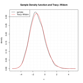
(a) Standard normal entries

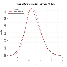
(b) Entry distribution: $\mathbb{P}(X=\sqrt{3})=\mathbb{P}(X=-\sqrt{3})=1/6$, $\mathbb{P}(X=0)=2/3$. Note $\mathbb{E}X=0$, $\mathbb{E}[X^{2}]=1$, $\mathbb{E}[X^{3}]=0$ and $\mathbb{E}[X^{4}]=3$, i.e., the first 4 moments of $X$ match those of the standard normal distribution.

Figure 1. Sample density function of the largest eigenvalue compared with the Tracy–Widom density function. The data matrix ${\mathbf{X}}$ has dimension $200\times 1000$. An ensemble of 2000 matrices is simulated.

Assuming (1.1) and iid entries $X_{it}$ with zero mean, unit variance and finite fourth moment, Geman [20] showed that

$$\dfrac{\lambda_{(1)}}{n}\stackrel{{\scriptstyle\rm a.s.}}{{\rightarrow}}\big{(}1+\sqrt{\gamma}\big{)}^{2}\,,\qquad n\to\infty\,.$$ (1.6)

Johnstone [25] complemented this strong law of large numbers by the corresponding central limit theorem in the special case of iid standard normal entries:

$$n^{2/3}\,\dfrac{(\sqrt{\gamma})^{1/3}}{\big{(}1+\sqrt{\gamma}\big{)}^{4/3}}\Big{(}\dfrac{\lambda_{(1)}}{n}-\big{(}1+\sqrt{\tfrac{p}{n}}\big{)}^{2}\Big{)}\stackrel{{\scriptstyle\rm d}}{{\rightarrow}}{\rm TW}\,,$$ (1.7)

where the limiting random variable has a Tracy–Widom distribution of order 1. Notice that the centering $\big{(}1+\sqrt{\tfrac{p}{n}}\big{)}^{2}$ can in general not be replaced by $(1+\sqrt{\gamma})^{2}$. This distribution is ubiquitous in random matrix theory. Its distribution function $F_{1}$ is given by

$$F_{1}(s)=\exp\Big{\{}-\frac{1}{2}\int_{s}^{\infty}[q(x)+(x-s)q^{2}(x)]\,\mathrm{d}x\Big{\}}\,,$$

where $q(x)$ is the unique solution to the Painlevé II differential equation

$$q^{\prime\prime}(x)=xq(x)+2q^{3}(x)\,,$$

where $q(x)\sim{\rm Ai}(x)$ as $x\to\infty$ and Ai$(\cdot)$ is the Airy kernel; see Tracy and Widom [35] for details. We notice that the rate $n^{2/3}$ compares favorably to the $\sqrt{n}$-rate in the classical central limit theorem for sums of iid finite variance random variables. The calculation of the spectrum is facilitated by the fact that the distribution of the classical Gaussian matrix ensembles is invariant under orthogonal transformations. The corresponding computation for non-invariant matrices with non-Gaussian entries is more complicated and was a major challenge for several years; a first step was made by Johansson [24]. Johnstone’s result was extended to matrices ${\mathbf{X}}$ with iid non-Gaussian entries by Tao and Vu [34, Theorem 1.16]. Assuming that the first four moments of the entry distribution match those of the standard normal distribution, they showed (1.7) by employing Lindeberg’s replacement method, i.e., the iid non-Gaussian entries are replaced step-by-step by iid Gaussian ones. This approach is well-known from summation theory for sequences of iid random variables. Tao and Vu’s result is a consequence of the so-called Four Moment Theorem, which describes the insensitivity of the eigenvalues with respect to changes in the distribution of the entries. To some extent (modulo the strong moment matching conditions) it shows the universality of Johnstone’s limit result (1.7). Later we will deal with entries with infinite fourth moment. In this case, the weak limit for the normalized largest eigenvalue $\lambda_{(1)}$ is distinct from the Tracy–Widom distribution: the classical Fréchet extreme value distribution appears. In Figure 1 we illustrate how the Tracy–Widom approximation works for Gaussian and non-Gaussian entries of ${\mathbf{X}}$ and in Figure 2 we also illustrate that this approach fails when $\mathbb{E}[X^{4}]=\infty$.

Figure 1 compares the sample density function of the properly normalized largest eigenvalue estimated from 2000 simulated sample covariance matrices ${\mathbf{X}}{\mathbf{X}}^{\prime}$ ($n=1000,p=200$) with the Tracy–Widom density. If $X$ has infinite fourth moment and further regularity conditions on the tail hold then the Tracy–Widom limiting law needs to be replaced by the Fréchet distribution; see Section 1.2 for details. Figure 2 illustrates this fact with a simulated ensemble whose entries are distributed according to the heavy-tailed distribution from (4.3) below with $\alpha=1.6$.

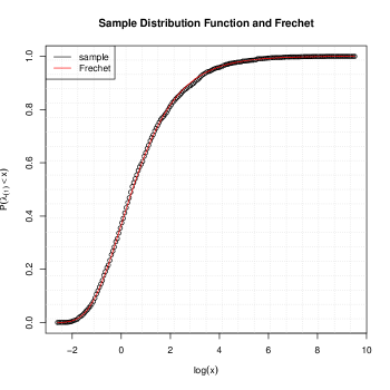
Figure 2. Sample distribution function of the largest eigenvalue $\lambda_{(1)}$ compared to the Fréchet distribution (solid line) with $\alpha=1.6$. The data matrices have dimension $200\times 1000$ and iid entries with infinite fourth moment. The results are based on 2000 replicates.

1.2. The heavy-tailed case

So far we focused on “light-tailed” ${\mathbf{X}}$ in the sense that its entries have finite fourth moment. However, there is statistical evidence that the assumption of finite fourth moment may be violated when dealing with data from insurance, finance or telecommunications. We illustrate this fact in Figure 3 where we show the pairs $(\alpha_{L},\alpha_{U})$ of lower and upper tail indices of $p=478$ log-return series composing the S&P 500 index estimated from $n=1,345$ daily observations from 01/04/2010 to 02/28/2015. This means we assume for every row $(X_{it})_{t=1,\ldots,n}$ of ${\mathbf{X}}$ that the tails behave like

$$\mathbb{P}(X_{it}>x)\sim c_{U}\,x^{-\alpha_{U}}\qquad\mbox{and}\qquad\mathbb{P}(X_{it}<-x)\sim c_{L}\,x^{-\alpha_{L}}\,,\qquad x\to\infty\,,$$

for non-negative constants $c_{L},c_{U}$. We apply the Hill estimator (see Embrechts et al. [17], p. 330, de Haan and Ferreira [13], p. 69) to the time series of the gains and losses in a naive way, neglecting the dependence and non-stationarity in the data; we also omit confidence bands. From the figure it is evident that the majority of the return series have tail indices below four, corresponding to an infinite fourth moment.

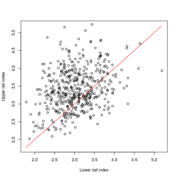
Figure 3. Tail indices of log-returns of 478 time series from the S&P 500 index. The values $(\hat{\alpha}_{L},\hat{\alpha}_{U})$ of the lower and upper tail indices are provided by Hill’s estimator. We also draw the line $\hat{\alpha}_{U}=\hat{\alpha}_{L}$.

The behavior of the largest eigenvalue $\lambda_{(1)}$ changes dramatically when ${\mathbf{X}}$ has infinite fourth moment. Bai and Silverstein [4] proved for an $n\times n$ matrix ${\mathbf{X}}$ with iid centered entries that

$$\limsup_{n\to\infty}\dfrac{\lambda_{(1)}}{n}=\infty\qquad{\rm a.s.}$$ (1.8)

This is in stark contrast to Geman’s result (1.6).

In the heavy-tailed case it is common to assume a regular variation condition:

$$\mathbb{P}(X>x)\sim p_{+}\,\dfrac{L(x)}{x^{\alpha}}\qquad\mbox{and}\qquad\mathbb{P}(X<-x)\sim p_{-}\,\dfrac{L(x)}{x^{\alpha}}\,,\qquad x\to\infty\,,$$ (1.9)

where $p_{\pm}$ are non-negative constants such that $p_{+}+p_{-}=1$ and $L$ is a slowly varying function. In particular, if $\alpha<4$ we have $\mathbb{E}[X^{4}]=\infty$. The regular variation condition on $X$ (we will also refer to $X$ as a regularly varying random variable) is needed for proving asymptotic theory for the eigenvalues of ${\mathbf{X}}{\mathbf{X}}^{\prime}$. This is similar to proving limit theory for sums of iid random variables with infinite variance stable limits; see for example Feller [19].

In (1.4) we have seen that the sequence $(F_{n^{-1}{\mathbf{X}}{\mathbf{X}}^{\prime}})$ of empirical spectral distributions converges to the Marčenko–Pastur law if the centered iid entries possess a finite second moment. Now we will discuss the situation when the entries are still iid and centered, but have an infinite variance. Here we assume the entries to be regularly varying with index $\alpha\in(0,2)$. Assuming (1.1) with $\gamma\in(0,1]$ in this infinite variance case, Belinschi et al. [5, Theorem 1.10] showed that the sequence $(F_{a_{n+p}^{-2}{\mathbf{X}}{\mathbf{X}}^{\prime}})$ converges with probability one to a non-random probability measure with density $\rho_{\alpha}^{\gamma}$ satisfying

$$\rho_{\alpha}^{\gamma}(x)x^{1+\alpha/2}\to\frac{\alpha\gamma}{2(1+\gamma)},\quad x\to\infty,$$

see also Ben Arous and Guionnet [7, Theorem 1.6]. The normalization $(a_{k})$ is chosen such that $\mathbb{P}(|X|>a_{k})\sim k^{-1}$ as $k\to\infty$. An application of the Potter bounds (see Bingham et al. [9, p. 25]) shows that $a_{n+p}^{2}/n\to\infty$.

It is interesting to note that there is a phase change in the extreme eigenvalues in going from finite to infinite fourth moment, while the phase change occurs for the empirical spectral distribution going from finite to infinite variance.

The theory for the largest eigenvalues of sample covariance matrices with heavy tails is less developed than in the light-tailed case. Pioneering work for $\lambda_{(1)}$ in the case of iid regularly varying entries $X_{it}$ with index $\alpha\in(0,2)$ is due to Soshnikov [32, 33]. He showed the point process convergence

$$N_{n}=\sum_{i=1}^{p}\varepsilon_{a_{np}^{-2}\lambda_{i}}\stackrel{{\scriptstyle\rm d}}{{\rightarrow}}N=\sum_{i=1}^{\infty}\varepsilon_{\Gamma_{i}^{-2/\alpha}}\,,\qquad n\to\infty\,,$$ (1.10)

under the growth condition (1.1) on $(p_{n})$. Here

$$\Gamma_{i}=E_{1}+\cdots+E_{i}\,,\qquad i\geq 1\,,$$ (1.11)

and $(E_{i})$ is an iid standard exponential sequence. In other words, $N$ is a Poisson point process on $(0,\infty)$ with mean measure $\mu(x,\infty)=x^{-\alpha/2}$, $x>0$. Convergence in distribution of point processes is understood in the sense of weak convergence in the space of point measures equipped with the vague topology; see Resnick [29, 30]. We can easily derive the limiting distribution of $a_{np}^{-2}\lambda_{(k)}$ for fixed $k\geq 1$ from (1.10):

$$\begin{split}\lim_{n\to\infty}\mathbb{P}(a_{np}^{-2}\lambda_{(k)}\leq x)&=\lim_{n\to\infty}\mathbb{P}(N_{n}(x,\infty)<k)=\mathbb{P}(N(x,\infty)<k)=\mathbb{P}(\Gamma_{k}^{-2/\alpha}\leq x)\\ &=\sum_{s=0}^{k-1}\frac{\big{(}\mu(x,\infty)\big{)}^{s}}{s!}\operatorname{e}^{-\mu(x,\infty)},\quad x>0.\end{split}$$

In particular,

$$\dfrac{\lambda_{(1)}}{a_{np}^{2}}\stackrel{{\scriptstyle\rm d}}{{\rightarrow}}\Gamma_{1}^{-\alpha/2}\,,\qquad n\to\infty\,,$$

where the limit has Fréchet distribution with parameter $\alpha/2$ and distribution function

$$\Phi_{\alpha/2}(x)={\rm e}\,^{-x^{-\alpha/2}}\,,\qquad x>0\,.$$

We mention that the tail balance condition (1.9) may be replaced in this case by the weaker assumption $\mathbb{P}(|X|>x)=L(x)x^{-\alpha}$ for a slowly varying function $L$. Indeed, it follows from the proof that only the squares $X_{it}^{2}$ contribute to the point process limits of the eigenvalues $(\lambda_{i})$. A consequence of the continuous mapping theorem and (1.10) is the joint convergence of the upper order statistics: for any $k\geq 1$,

$$a_{np}^{-2}\big{(}\lambda_{(1)},\ldots,\lambda_{(k)}\big{)}\stackrel{{\scriptstyle\rm d}}{{\rightarrow}}\big{(}\Gamma_{1}^{-2/\alpha},\ldots,\Gamma_{k}^{-2/\alpha}\big{)}\,,\qquad n\to\infty\,.$$

It follows from standard theory for point processes with iid points (e.g. Resnick [29, 30]) that (1.10) remains valid if we replace $N_{n}$ by the point process $\sum_{i=1}^{p}\sum_{t=1}^{n}\varepsilon_{X_{it}^{2}/a_{np}^{2}}$. Then we also have for any $k\geq 1$,

$$a_{np}^{-2}\big{(}X_{(1),np}^{2},\ldots,X_{(k),np}^{2}\big{)}\stackrel{{\scriptstyle\rm d}}{{\rightarrow}}\big{(}\Gamma_{1}^{-2/\alpha},\ldots,\Gamma_{k}^{-2/\alpha}\big{)}\,,\qquad n\to\infty\,,$$ (1.12)

where

$$X_{(1),np}^{2}\geq\cdots\geq X_{(np),np}^{2}$$

denote the order statistics of $(X_{it}^{2})_{i=1,\ldots,p;t=1,\ldots,n}$.

Auffinger et al. [2] showed that (1.10) remains valid under the regular variation condition (1.9) for $\alpha\in(2,4)$, the growth condition (1.1) on $(p_{n})$ and the additional assumption $\mathbb{E}[X]=0$. Of course, (1.12) remains valid as well. Davis et al. [12] extended these results to the case when the rows of ${\mathbf{X}}$ are iid linear processes with iid regularly varying noise. The Poisson point process convergence result of (1.10) remains valid in this case. Different limit processes can only be expected if there is dependence across rows and columns.

In what follows, we refer to the heavy-tailed case when we assume the regular variation condition (1.9) for some $\alpha\in(0,4)$.

1.3. Overview

The primary objective of this overview is to make a connection between extreme value theory and the behavior of the largest eigenvalues of sample covariance matrices from heavy-tailed multivariate time series. For time series that are linearly dependent through time and across rows, it turns out that the extreme eigenvalues are essentially determined by the extreme order statistics from an array of iid random variables. The asymptotic behavior of the extreme eigenvalues is then derived routinely from classical extreme value theory. As such, explicit joint distributions of the extreme order statistics can be given which yield a plethora of ancillary results. Convergence of the point process of extreme eigenvalues, properly normalized, plays a central role in establishing the main results.

In Section 2 we continue the study of the case when the data matrix ${\mathbf{X}}$ consists of iid heavy-tailed entries. We will consider power-law growth rates on the dimension $(p_{n})$ that is more general than prescribed by (1.1). In Section 3 we introduce a model for $X_{it}$ which allows for linear dependence across the rows and through time. The point process convergence of normalized eigenvalues is presented in Section 3.4. This result lays the foundation for new insight into the spectral behavior of the sample covariance matrix, which is the content of Section 4.1.

Sections 4.1 and 4.3 are devoted to sample autocovariance matrices. Motivated by [26], we study the eigenvalues of sums of transformed matrices and illustrate the results in two examples. These results are applied to the time series of S&P 500 in Section 4.2. Appendix A contains useful facts about regular variation and point processes.

2. General growth rates for $p_{n}$ in the iid heavy-tailed case

This section is based on ideas in Heiny and Mikosch [21] where one can also find detailed proofs.

Growth conditions on $(p_{n})$

In many applications it is not realistic to assume that the dimension $p$ of the data and the sample size $n$ grow at the same rate. The aforementioned results of Soshnikov [32, 33] and Auffinger et al. [2] already indicate that the value $\gamma$ in the growth rate (1.1) does not appear in the distributional limits. This obervation is in contrast to the light-tailed case; see (1.6) and (1.7). Davis et al. [11, 12] and Heiny and Mikosch  [21] allowed for more general rates for $p_{n}\to\infty$ than linear growth in $n$. Recall that $p=p_{n}\to\infty$ is the number of rows in the matrix ${\mathbf{X}}_{n}$. We need to specify the growth rate of $(p_{n})$ to ensure a non-degenerate limit distribution of the normalized singular values of the sample autocovariance matrices. To be precise, we assume

$$p=p_{n}=n^{\beta}\ell(n),\quad n\geq 1, C_{p}(\beta)$$ ()

where $\ell$ is a slowly varying function and $\beta\geq 0$. If $\beta=0$, we also assume $\ell(n)\to\infty$. Condition $C_{p}(\beta)$ is more general than the growth conditions in the literature; see [2, 11, 12].

Theorem 2.1.

Assume that ${\mathbf{X}}={\mathbf{X}}_{n}$ has iid entries satisfying the regular variation condition (1.9) for some $\alpha\in(0,4)$. If $\mathbb{E}[|X|]<\infty$ we also suppose that $\mathbb{E}[X]=0$. Let $(p_{n})$ be an integer sequence satisfying $C_{p}(\beta)$ with $\beta\geq 0$. In addition, we require

$$\min(\beta,\beta^{-1})\in(\alpha/2-1,1]\qquad\mbox{ for }\alpha\in[2,4), \widetilde{C}_{\beta}(\alpha)$$ ()

Then

$$\sum_{i=1}^{p}\varepsilon_{a_{np}^{-2}\lambda_{i}}\stackrel{{\scriptstyle\rm d}}{{\rightarrow}}\sum_{i=1}^{\infty}\varepsilon_{\Gamma_{i}^{-2/\alpha}}\,,\qquad n\to\infty\,,$$ (2.1)

where the convergence holds in the space of point measures with state space $(0,\infty)$ equipped with the vague toplogy; see Resnick [29].

A discussion of the case $\beta\in[0,1]$

We mentioned earlier that in the heavy-tailed case, limit theory for the largest eigenvalues of the sample covariance matrix is rather insensitive to the growth rate of $(p_{n})$ and that the limits are essentially determined by the diagonal of this matrix. This is confirmed by the following result.

Proposition 2.2.

Assume that ${\mathbf{X}}={\mathbf{X}}_{n}$ has iid entries satisfying the regular variation condition (1.9) for some $\alpha\in(0,4)$. If $\mathbb{E}[|X|]<\infty$ we also suppose that $\mathbb{E}[X]=0$. Then for any sequence $(p_{n})$ satisfying $C_{p}(\beta)$ with $\beta\in[0,1]$ we have

$$a_{np}^{-2}\|{\mathbf{X}}{\mathbf{X}}^{\prime}-\operatorname{diag}({\mathbf{X}}{\mathbf{X}}^{\prime})\|_{2}\stackrel{{\scriptstyle\mathbb{P}}}{{\rightarrow}}0\,,\qquad n\to\infty\,,$$

where $\|\cdot\|_{2}$ denotes the spectral norm; see (3.10) for its definition.

Proposition 2.2 is not unexpected for two reasons:

• It is well-known from classical theory (see Embrechts and Veraverbeke [18]) that for any iid regularly varying non-negative random variables $Y,Y^{\prime}$ with index $\alpha^{\prime}>0$, $Y\,Y^{\prime}$ is regularly varying with index $\alpha^{\prime}$ while $Y^{2}$ is regularly varying with index $\alpha^{\prime}/2$. Therefore $X^{2}$ and $X_{11}X_{12}$ are regularly varying with indices $\alpha/2$ and $\alpha$, respectively.

• The aforementioned tail behavior is inherited by the entries of ${\mathbf{X}}{\mathbf{X}}^{\prime}$ in the following sense. By virtue of Nagaev-type large deviation results for an iid regularly varying sequence $(Y_{i})$ with index $\alpha^{\prime}\in(0,2)$ where we also assume that $\mathbb{E}[Y_{0}]=0$ if $\mathbb{E}[|Y_{0}|]<\infty$ (see Theorem A.1) we have that $\mathbb{P}(Y_{1}+\cdots+Y_{n}>b_{n})/(n\,\mathbb{P}(|Y_{0}|>b_{n}))$ converges to a non-negative constant provided $b_{n}/a_{n}^{\prime}\to\infty$, where $\mathbb{P}(|Y_{0}|>a_{n}^{\prime})\sim n^{-1}$ as $n\to\infty$. As a consequence of the tail behaviors of $X_{it}^{2}$ and $X_{it}X_{jt}$ for $i\neq j$ and Nagaev’s results we have for $(b_{n})$ such that $b_{n}/a_{n}^{2}\to\infty$,

  $$\dfrac{\mathbb{P}\big{(}({\mathbf{X}}{\mathbf{X}}^{\prime})_{ij}>b_{n}\big{)}}{\mathbb{P}\big{(}({\mathbf{X}}{\mathbf{X}}^{\prime})_{ii}-c_{n}>b_{n}\big{)}}\sim\dfrac{n\,\mathbb{P}(X_{11}X_{12}>b_{n})}{n\,\mathbb{P}(X^{2}>b_{n})}\to 0\,,\qquad n\to\infty\,,$$

  where $c_{n}=0$ or $n\,\mathbb{E}[X^{2}]$ according as $\alpha\in(0,2)$ or $\alpha\in(2,4)$. This means that the diagonal and off-diagonal entries of ${\mathbf{X}}{\mathbf{X}}^{\prime}$ inherit the tails of $X_{it}^{2}$ and $X_{it}X_{jt}$, $i\neq j$, respectively, above the high threshold $b_{n}$.

Proposition 2.2 has some immediate consequences for the approximation of the eigenvalues of ${\mathbf{X}}{\mathbf{X}}^{\prime}$ by those of ${\rm diag}({\mathbf{X}}{\mathbf{X}}^{\prime})$. Indeed, let $C$ be a symmetric $p\times p$ matrix with eigenvalues $\lambda_{1}(C),\ldots,\lambda_{p}(C)$ and ordered eigenvalues

$$\lambda_{(1)}(C)\geq\cdots\geq\lambda_{(p)}(C)\,.$$ (2.2)

Then for any symmetric $p\times p$ matrices $A,B$, by Weyl’s inequality (see Bhatia [8]),

$$\max_{i=1,\ldots,p}\big{|}\lambda_{(i)}(A+B)-\lambda_{(i)}(A)\big{|}\leq\|B\|_{2}\,.$$

If we now choose $A+B={\mathbf{X}}{\mathbf{X}}^{\prime}$ and $A=\operatorname{diag}({\mathbf{X}}{\mathbf{X}}^{\prime})$ we obtain the following result.

Corollary 2.3.

Under the conditions of Proposition 2.2,

$$a_{np}^{-2}\,\max_{i=1,\ldots,p}\big{|}\lambda_{(i)}-\lambda_{(i)}(\operatorname{diag}({\mathbf{X}}{\mathbf{X}}^{\prime}))\big{|}\stackrel{{\scriptstyle\mathbb{P}}}{{\rightarrow}}0\,,\quad n\to\infty\,.$$

Thus the problem of deriving limit theory for the order statistics of ${\mathbf{X}}{\mathbf{X}}^{\prime}$ has been reduced to limit theory for the order statistics of the iid row-sums

$$D_{i}^{\rightarrow}=({\mathbf{X}}{\mathbf{X}}^{\prime})_{ii}=\sum_{t=1}^{n}X_{it}^{2}\,,\qquad i=1,\ldots,p\,,$$

which are the eigenvalues of $\operatorname{diag}({\mathbf{X}}{\mathbf{X}}^{\prime})$. This theory is completely described by the point processes constructed from the points $D_{i}^{\rightarrow}/a_{np}^{2}$ $i=1,\ldots,p$. Necessary and sufficient conditions for the weak convergence of these point processes are provided by Lemma A.2 which in combination with the Nagaev-type large deviation results of Theorem A.1 yield the following result; see also Davis et al. [11].

Lemma 2.4.

Assume the conditions of Proposition 2.2 hold. Then

$$\sum_{i=1}^{p}\varepsilon_{a_{np}^{-2}(D_{i}^{\rightarrow}-c_{n})}\stackrel{{\scriptstyle\rm d}}{{\rightarrow}}\sum_{i=1}^{\infty}\varepsilon_{\Gamma_{i}^{-2/\alpha}}\,,\qquad n\to\infty\,,$$

where $(\Gamma_{i})$ is defined in (1.11) and $c_{n}=0$ if $\mathbb{E}[D^{\rightarrow}]=\infty$ and $c_{n}=\mathbb{E}[D^{\rightarrow}]$ otherwise.

In this result, centering is only needed for $\alpha\in[2,4)$ when $n/a_{np}^{2}\not\to 0$. Under the additional condition $\widetilde{C}_{\beta}(\alpha)$, $n/a_{np}^{2}\to 0$ in view of the Potter bounds; see Bingham et al. [9, p. 25]. Combining Lemma 2.4 and Corollary 2.3, we conclude that Theorem 2.1 holds for $\beta\in[0,1]$.

Extension to general $\beta$

Next we explain that it suffices to consider only the case $\beta\in[0,1]$ and how to proceed when $\beta>1$. The main reason is that the $p\times p$ sample covariance matrix ${\mathbf{X}}{\mathbf{X}}^{\prime}$ and the $n\times n$ matrix ${\mathbf{X}}^{\prime}{\mathbf{X}}$ have the same rank and their non-zero eigenvalues coincide; see Bhatia [8, p. 64]. When proving limit theory for the eigenvalues of the sample covariance matrix one may switch to ${\mathbf{X}}^{\prime}{\mathbf{X}}$ and vice versa, hereby interchanging the roles of $p$ and $n$. By switching to ${\mathbf{X}}^{\prime}{\mathbf{X}}$, one basically replaces $\beta$ by $\beta^{-1}$. Since $\min(\beta,\beta^{-1})\in[0,1]$ for any $\beta\geq 0$, one can assume without loss of generality that $\beta\in[0,1]$. This trick allows one to extend results for $(p_{n})$ satisfying $C_{p}(\beta)$ with $\beta\in[0,1]$ to $\beta>1$. We illustrate this approach by providing the direct analogs of Proposition 2.2 and Corollary 2.3.

Proposition 2.5.

Assume that ${\mathbf{X}}={\mathbf{X}}_{n}$ has iid entries satisfying the regular variation condition (1.9) for some $\alpha\in(0,4)$. If $\mathbb{E}[|X|]<\infty$ we also suppose that $\mathbb{E}[X]=0$. Then for any sequence $(p_{n})$ satisfying $C_{p}(\beta)$ with $\beta>1$ we have

$$a_{np}^{-2}\|{\mathbf{X}}^{\prime}{\mathbf{X}}-\operatorname{diag}({\mathbf{X}}^{\prime}{\mathbf{X}})\|_{2}\stackrel{{\scriptstyle\mathbb{P}}}{{\rightarrow}}0\,,\qquad n\to\infty\,,$$

where $\|\cdot\|_{2}$ denotes the spectral norm.

Note that for $\beta>1$ we have $\lim_{n\to\infty}p/n=\infty$. This means that ${\mathbf{X}}^{\prime}{\mathbf{X}}$ has asymptotically a much smaller dimension than ${\mathbf{X}}{\mathbf{X}}^{\prime}$ and therefore it is more convenient to work with ${\mathbf{X}}^{\prime}{\mathbf{X}}$ when bounding the spectral norm.

Corollary 2.6.

Under the conditions of Proposition 2.5,

$$a_{np}^{-2}\,\max_{i=1,\ldots,n}\big{|}\lambda_{(i)}-\lambda_{(i)}(\operatorname{diag}({\mathbf{X}}^{\prime}{\mathbf{X}}))\big{|}\stackrel{{\scriptstyle\mathbb{P}}}{{\rightarrow}}0\,,\quad n\to\infty\,.$$

Now, Theorem 2.1 for $\beta>1$ is a consequence of Corollary 2.6.

3. Introducing dependence between the rows and columns

For details on the results of this section, we refer to Davis et al. [11], Heiny and Mikosch [21] and Heiny et al. [22].

3.1. The model

When dealing with covariance matrices of a multivariate time series $({\mathbf{X}}_{n})$ it is rather natural to assume dependence between the entries $X_{it}$. In this section we introduce a model which allows for linear dependence between the rows and columns of ${\mathbf{X}}$:

$$X_{it}=\sum_{l\in\mathbb{Z}}\sum_{k\in\mathbb{Z}}h_{kl}Z_{i-k,t-l}\,,\qquad i,t\in\mathbb{Z}\,,$$ (3.1)

where $(Z_{it})_{i,t\in\mathbb{Z}}$ is a field of iid random variables and $(h_{kl})_{k,l\in\mathbb{Z}}$ is an array of real numbers. Of course, linear dependence is restrictive in some sense. However, the particular dependence structure allows one to determine those ingredients in the sample covariance matrix which contribute to its largest eigenvalues. If the series in (3.1) converges a.s. $(X_{it})$ constitutes a strictly stationary random field. We denote generic elements of the $Z$- and $X$-fields by $Z$ and $X$, respectively. We assume that $Z$ is regularly varying in the sense that

$$\mathbb{P}(Z>x)\sim p_{+}\dfrac{L(x)}{x^{\alpha}}\quad\mbox{and}\quad\mathbb{P}(Z\leq-x)\sim p_{-}\dfrac{L(x)}{x^{\alpha}}\,,\qquad x\to\infty\,,$$ (3.2)

for some tail index $\alpha>0$, constants $p_{+},p_{-}\geq 0$ with $p_{+}+p_{-}=1$ and a slowly varying $L$. We will assume $\mathbb{E}[Z]=0$ whenever $\mathbb{E}[Z^{2}]<\infty$. Moreover, we require the summability condition

$$\sum_{l\in\mathbb{Z}}\sum_{k\in\mathbb{Z}}|h_{kl}|^{\delta}<\infty$$ (3.3)

for some $\delta\in(0,\min({\alpha/2},1))$ which ensures the a.s. absolute convergence of the series in (3.1). Under the conditions (3.2) and (3.3), the marginal and finite-dimensional distributions of the field $(X_{it})$ are regularly varying with index $\alpha$; see Embrechts et al. [17], Appendix A3.3. Therefore we also refer to $(X_{it})$ and $(Z_{it})$ as regularly varying fields.

The model (3.1) was introduced by Davis et al. [12], assuming the rows iid, and in the present form by Davis et al. [11].

3.2. Sample covariance and autocovariance matrices

From the field $(X_{it})$ we construct the $p\times n$ matrices

$${\mathbf{X}}_{n}(s)=(X_{i,t+s})_{i=1,\ldots,p;t=1,\ldots,n}\,,\qquad s=0,1,2,\ldots\,,$$ (3.4)

As before, we will write ${\mathbf{X}}={\mathbf{X}}_{n}(0)$. Now we can introduce the (non-normalized) sample autocovariance matrices

$${\mathbf{X}}_{n}(0){\mathbf{X}}_{n}(s)^{\prime}\,,\qquad s=0,1,2,\ldots\,.$$ (3.5)

We will refer to $s$ as the lag. For $s=0$, we obtain the sample covariance matrix. In what follows, we will be interested in the asymptotic behavior (of functions) of the eigen- and singular values of the sample covariance and autocovariance matrices in the heavy-tailed case. Recall that the singular values of a matrix $A$ are the square roots of the eigenvalues of the non-negative definite matrix $AA^{\prime}$ and its spectral norm $\|A\|_{2}$ is its largest singular value. We notice that ${\mathbf{X}}_{n}(0){\mathbf{X}}_{n}(s)^{\prime}$ is not symmetric and therefore its eigenvalues can be complex. To avoid this situation, we use the squares

$${\mathbf{X}}_{n}(0){\mathbf{X}}_{n}(s)^{\prime}{\mathbf{X}}_{n}(s){\mathbf{X}}_{n}(0)^{\prime}$$ (3.6)

whose eigenvalues are the squares of the singular values of ${\mathbf{X}}_{n}(0){\mathbf{X}}_{n}(s)^{\prime}$. The idea of using the sample autocovariance matrices and functions of their squares (3.6) originates from a paper by Lam and Yao [26] who used a model different from (3.1). This idea is quite natural in the context of time series analysis.

In Theorem 3.1 below, we provide a general approximation result for the ordered singular values of the sample autocovariance matrices in the heavy-tailed case. This result is rather technical. To formulate it we introduce further notation. As before, $p=p_{n}$ is any integer sequence converging to infinity.

3.3. More notation

Important roles are played by the quantities $(Z_{it}^{2})_{i=1,\ldots,p;t=1,\ldots,n}$ and their order statistics

$$Z_{(1),np}^{2}\geq Z_{(2),np}^{2}\geq\ldots\geq Z_{(np),np}^{2},\qquad n,p\geq 1\,.$$ (3.7)

As important are the row-sums

$$D_{i}^{\rightarrow}=D_{i}^{(n),\rightarrow}=\sum_{t=1}^{n}Z_{it}^{2}\,,\qquad i=1,\ldots,p;\quad n=1,2,\ldots\,,$$ (3.8)

with generic element $D^{\rightarrow}$ and their ordered values

$$D_{(1)}^{\rightarrow}=D_{L_{1}}^{\rightarrow}\geq\cdots\geq D_{(p)}^{\rightarrow}=D_{L_{p}}^{\rightarrow}\,,$$ (3.9)

where we assume without loss of generality that $(L_{1},\ldots,L_{p})$ is a permutation of $(1,\ldots,p)$ for fixed $n$.

Finally, we introduce the column-sums

$$D_{t}^{\downarrow}=D_{t}^{(n),\downarrow}=\sum_{i=1}^{p}Z_{it}^{2}\,,\qquad t=1,\ldots,n;\;\quad p=1,2,\ldots\,,$$

with generic element $D^{\downarrow}$ and we also adapt the notation from (3.9) to these quantities.

Matrix norms

For any $p\times n$ matrix ${\mathbf{A}}=(a_{ij})$, we will use the following norms:

• Spectral norm:

  $$\|{\mathbf{A}}\|_{2}=\sqrt{\lambda_{(1)}({\mathbf{A}}{\mathbf{A}}^{\prime})}\,,$$ (3.10)

• Frobenius norm:

  $$\|{\mathbf{A}}\|_{F}=\Big{(}\sum_{i=1}^{p}\sum_{j=1}^{n}|a_{ij}|^{2}\Big{)}^{1/2}\,.$$

We will frequently make use of the bound $\|{\mathbf{A}}\|_{2}\leq\|{\mathbf{A}}\|_{F}$. Standard references for matrix norms are [6, 8, 23, 31].

Singular values of the sample autocovariance matrices

Fix integers $n\geq 1$ and $s\geq 0$. We recycle the $\lambda$-notation for the singular values $\lambda_{1}(s),\ldots,\lambda_{p}(s)$ of the sample autocovariance matrix ${\mathbf{X}}_{n}(0){\mathbf{X}}_{n}(s)^{\prime}$, suppressing the dependence on $n$. Correspondingly, the order statistics are denoted by

$$\lambda_{(1)}(s)\geq\cdots\geq\lambda_{(p)}(s)\,.$$ (3.11)

When $s=0$ we typically write $\lambda_{i}$ instead of $\lambda_{i}(0)$.

The matrix ${\mathbf{M}}(s)$

We introduce some auxiliary matrices derived from the coefficient matrix ${\mathbf{H}}=(h_{kl})_{k,l\in\mathbb{Z}}$:

$${\mathbf{H}}(s)=(h_{k,l+s})_{k,l\in\mathbb{Z}},\qquad{\mathbf{M}}(s)={\mathbf{H}}(0){\mathbf{H}}(s)^{\prime}\qquad s\geq 0\,.$$

Notice that

$$({\mathbf{M}}(s))_{ij}=\sum_{l\in\mathbb{Z}}h_{i,l}h_{j,l+s},\qquad i,j\in\mathbb{Z}.$$ (3.12)

We denote the ordered singular values of ${\mathbf{M}}(s)$ by

$$v_{1}(s)\geq v_{2}(s)\geq\cdots\,.$$ (3.13)

Let $r(s)$ be the rank of ${\mathbf{M}}(s)$ so that $v_{r(s)}(s)>0$ while $v_{r(s)+1}(s)=0$ if $r(s)$ is finite, otherwise $v_{i}(s)>0$ for all $i$. We also write $r=r(0)$.

Under the summability condition (3.3) on $(h_{kl})$ for fixed $s\geq 0$,

$$\sum_{i=1}^{\infty}(v_{i}(s))^{2} = \|{\mathbf{M}}(s)\|_{F}^{2}=\sum_{i,j\in\mathbb{Z}}\sum_{l_{1},l_{2}\in\mathbb{Z}}h_{i,l_{1}}h_{j,l_{1}+s}h_{i,l_{2}}h_{j,l_{2}+s}$$ (3.14)

$$\leq c\,\Big{(}\sum_{l_{1},l_{2}\in\mathbb{Z}}\sum_{i\in\mathbb{Z}}|h_{i,l_{1}}h_{i,l_{2}}|\Big{)}^{2}\leq c\,\sum_{l_{1}\in\mathbb{Z}}\sum_{i\in\mathbb{Z}}|h_{i,l_{1}}|<\infty\,.$$

Therefore all singular values $v_{i}(s)$ are finite and the ordering (3.13) is justified.

Here and in what follows, we write $c$ for any constant whose value is not of interest.

Normalizing sequence

We define $(a_{k})$ by

$$\mathbb{P}(|Z|>a_{k})\sim k^{-1}\,,\qquad k\to\infty\,,$$

and choose the normalizing sequence for the singular values as $(a_{np}^{2})$ for suitable sequences $p=p_{n}\to\infty$.

Approximations to singular values

We will give approximations to the singular values $\lambda_{i}(s)$ in terms of the $p$ largest ordered values for $s\geq 0$,

$$\delta_{(1)}(s)\geq\cdots\geq\delta_{(p)}(s)\,,$$

$$\gamma_{(1)}^{\rightarrow}(s)\geq\cdots\geq\gamma_{(p)}^{\rightarrow}(s)\,,$$

$$\gamma_{(1)}^{\downarrow}(s)\geq\cdots\geq\gamma_{(n)}^{\downarrow}(s)\,,$$

from the sets

$$\big{\{}Z_{(i),np}^{2}v_{j}(s)\,,i=1,\ldots,p\,;j=1,2,\ldots\big{\}}\,,$$

$$\big{\{}D_{i}^{\rightarrow}v_{j}(s),i=1,\ldots,p\,;j=1,2,\ldots\big{\}}\,,$$

$$\big{\{}D_{t}^{\downarrow}v_{j}(s),t=1,\ldots,n\,;j=1,2,\ldots\big{\}}\,,$$

respectively.

3.4. Approximation of the singular values

In the following result we povide some useful approximations to the singular values of the sample autocovariance matrices of the linear model (3.1).

Theorem 3.1.

Consider the linear process (3.1) under

• the regular variation condition (3.2) for some $\alpha\in(0,4)$,

• the centering condition $\mathbb{E}[Z]=0$ if $\mathbb{E}[|Z|]<\infty$,

• the summability condition (3.3) on the coefficient matrix $(h_{kl})$,

• the growth condition $C_{p}(\beta)$ on $(p_{n})$ for some $\beta\geq 0$.

Then the following statements hold for $s\geq 0$:

1. We consider two disjoint cases: $\alpha\in(0,2)$ and $\beta\in(0,\infty)$, or $\alpha\in[2,4)$ and $\beta$ satisfying $\widetilde{C}_{\beta}(\alpha)$. Then

   $$a_{np}^{-2}\max_{i=1,\ldots,p}|\lambda_{(i)}(s)-\delta_{(i)}(s)|\stackrel{{\scriptstyle\mathbb{P}}}{{\rightarrow}}0,\quad n\to\infty.$$ (3.15)

2. Assume $\beta\in[0,1]$. If $\alpha\in(0,2]$, $\mathbb{E}[Z^{2}]=\infty$ or $\alpha\in[2,4)$, $\mathbb{E}[Z^{2}]<\infty$ and $\beta\in(\alpha/2-1,1]$ then

   $$a_{np}^{-2}\max_{i=1,\ldots,p}|\lambda_{(i)}(s)-\gamma_{(i)}^{\rightarrow}(s)|\stackrel{{\scriptstyle\mathbb{P}}}{{\rightarrow}}0,\quad n\to\infty.$$

   Assume $\beta>1$. If $\alpha\in(0,2]$, $\mathbb{E}[Z^{2}]=\infty$ or $\alpha\in[2,4)$, $\mathbb{E}[Z^{2}]<\infty$ and $\beta^{-1}\in(\alpha/2-1,1]$. Then

   $$a_{np}^{-2}\max_{i=1,\ldots,p}|\lambda_{(i)}(s)-\gamma_{(i)}^{\downarrow}(s)|\stackrel{{\scriptstyle\mathbb{P}}}{{\rightarrow}}0,\quad n\to\infty.$$

Remark 3.2.

The proof of Theorem 3.1 is given in Heiny et al. [22]. Part (2) of this result with more restrictive conditions on the growth rate of $(p_{n})$ is contained in Davis et al. [11]. These proofs are very technical and lengthy.

Remark 3.3.

If we consider a random array $(h_{kl})$ independent of $(X_{it})$ and assume that the summability condition (3.3) holds a.s. then Theorem 3.1 remains valid conditionally on $(h_{kl})$, hence unconditionally in $\mathbb{P}$-probability; see also [11].

3.5. Point process convergence

Theorem 3.1 and arguments similar to the proofs in Davis et al. [11] enable one to derive the weak convergence of the point processes of the normalized singular values. Recall the representation of the points $(\Gamma_{i})$ of a unit rate homogeneous Poisson process on $(0,\infty)$ given in (1.11). For $s\geq 0$, we define the point processes of the normalized singular values:

$$N_{n}^{\lambda,s}=\sum_{i=1}^{p}\varepsilon_{a_{np}^{-2}(\lambda_{(i)}(0),\ldots,\lambda_{(i)}(s))}\,.$$ (3.16)

Theorem 3.4.

Assume the conditions of Theorem 3.1. Then $(N_{n}^{\lambda,s})$ converge weakly in the space of point measures with state space $(0,\infty)^{s+1}$ equipped with the vague topology. If either $\alpha\in(0,2]$, $\mathbb{E}[Z^{2}]=\infty$ and $\beta\geq 0$, or $\alpha\in[2,4)$, $\mathbb{E}[Z^{2}]<\infty$ and $\widetilde{C}_{\beta}(\alpha)$ hold then

$$N_{n}^{\lambda,s}\stackrel{{\scriptstyle d}}{{\rightarrow}}N=\sum_{i=1}^{\infty}\sum_{j=1}^{\infty}\varepsilon_{\Gamma_{i}^{-2/\alpha}(v_{j}(0),\ldots,v_{j}(s))},\qquad n\to\infty.$$ (3.17)

Proof.

Regular variation of $Z^{2}$ is equivalent to

$$n\,p\,\mathbb{P}(a_{np}^{-2}Z^{2}\in\cdot)\stackrel{{\scriptstyle v}}{{\rightarrow}}\mu(\cdot),$$ (3.18)

where $\stackrel{{\scriptstyle v}}{{\rightarrow}}$ denotes vague convergence of Radon measures on $(0,\infty)$ and the measure $\mu$ is given by $\mu(x,\infty)=x^{-\alpha/2}$, $x>0$. In view of Resnick [30], Proposition 3.21, (3.18) is equivalent to the weak convergence of the following point processes:

$$\sum_{i=1}^{p}\sum_{t=1}^{n}\varepsilon_{a_{np}^{-2}Z_{it}^{2}}=\sum_{i=1}^{np}\varepsilon_{a_{np}^{-2}Z^{2}_{(i),np}}\stackrel{{\scriptstyle d}}{{\rightarrow}}\sum_{i=1}^{\infty}\varepsilon_{\Gamma_{i}^{-2/\alpha}}=\widetilde{N}\,,\quad n\to\infty\,,$$

where the limit $\widetilde{N}$ is a Poisson random measure (PRM) with state space $(0,\infty)$ and mean measure $\mu$.

Since $a_{np}^{-2}Z^{2}_{(p),np}\stackrel{{\scriptstyle\mathbb{P}}}{{\rightarrow}}0$ as $n\to\infty$, the point processes $\sum_{i=1}^{p}\varepsilon_{a_{np}^{-2}Z^{2}_{(i),np}}$ converge weakly to the same PRM:

$$\sum_{i=1}^{p}\varepsilon_{a_{np}^{-2}Z^{2}_{(i),np}}\stackrel{{\scriptstyle d}}{{\rightarrow}}\sum_{i=1}^{\infty}\varepsilon_{\Gamma_{i}^{-2/\alpha}}\,,\quad n\to\infty\,.$$ (3.19)

A continuous mapping argument together with the fact that $\sum_{i=1}^{\infty}(v_{i}(s))^{2}<\infty$ (see (3.14)) shows that

$$\sum_{j=1}^{\infty}\sum_{i=1}^{p}\varepsilon_{a_{np}^{-2}Z^{2}_{(i),np}(v_{j}(0),\ldots,v_{j}(s))}\stackrel{{\scriptstyle d}}{{\rightarrow}}\sum_{j=1}^{\infty}\sum_{i=1}^{\infty}\varepsilon_{\Gamma_{i}^{-2/\alpha}(v_{j}(0),\ldots,v_{j}(s))}\,.$$

If the assumptions of part (1) of Theorem 3.1 are satisfied an application of (3.15) (also recalling the definition of $(\delta_{(i)}(s))$) shows that (3.19) remains valid with the points $(a_{np}^{-2}Z^{2}_{(i),np}(v_{j}(0),\ldots,v_{j}(s)))$ replaced by $(a_{np}^{-2}(\lambda_{(i)}(0),\ldots,\lambda_{(i)}(s))$.

The only cases which are not covered by Theorem 3.1(1) are $\alpha\in(0,2)$, $\beta=0$ and $\alpha=2$, $\mathbb{E}[Z^{2}]=\infty$, $\beta\geq 0$. In these cases we get from Theorem A.1 that

$$p\,\mathbb{P}(a_{np}^{-2}D^{\rightarrow}>x)\sim p\,n\,\mathbb{P}(Z^{2}>a_{np}^{2}x)\to\mu(x,\infty)\,,\quad x>0\,,$$

i.e., $p\,\mathbb{P}(a_{np}^{-2}D^{\rightarrow}\in\cdot)\stackrel{{\scriptstyle v}}{{\rightarrow}}\mu(\cdot)$. It follows from Lemma A.2 that $\sum_{i=1}^{p}\varepsilon_{a_{np}^{-2}D_{i}^{\rightarrow}}\stackrel{{\scriptstyle\rm d}}{{\rightarrow}}\widetilde{N}$. As before, a continuous mapping argument in combination with the approximation obtained in Theorem 3.1(2) justifies the replacement of the points $(a_{np}^{-2}D_{(i)}^{\rightarrow}(v_{j}(0),\ldots,v_{j}(s)))$ by $(a_{np}^{-2}(\lambda_{(i)}(0),\ldots,\lambda_{(i)}(s)))$ in the case $\beta\in[0,1]$. If $\beta>1$ one has to work with the quantities $(D_{i}^{\downarrow})_{i=1,\ldots,n}$ instead of $(D_{i}^{\rightarrow})_{i=1,\ldots,p}$ and one may follow the same argument as above. This finishes the proof. ∎

4. Some applications

4.1. Sample covariance matrices

The sample covariance matrix ${\mathbf{X}}_{n}(0){\mathbf{X}}_{n}(0)^{\prime}={\mathbf{X}}{\mathbf{X}}^{\prime}$ is a non-negative definite matrix. Therefore its eigenvalues and singular values coincide. Moreover, $v_{j}=v_{j}(0)$, $j\geq 1$, are the eigenvalues of ${\mathbf{M}}={\mathbf{M}}(0)$.

Theorem 3.1(1) yields an approximation of the ordered eigenvalues $(\lambda_{(i)})$ of ${\mathbf{X}}{\mathbf{X}}^{\prime}$ by the quantities $(\delta_{(i)})$ which are derived from the order statistics of $(Z_{it}^{2})$. Part (2) of this result provides an approximation of $(\lambda_{(i)})$ by the quantities $(\gamma_{(i)}^{\rightarrow/\downarrow})$ which are derived from the order statistics of the partial sums $(D_{i}^{\rightarrow/\downarrow})$.

In the following example we illustrate the quality of the two approximations.

Example 4.1.

We choose a Pareto-type distribution for $Z$ with density

$$f_{Z}(x)=\left\{\begin{array}[]{cc}\frac{\alpha}{(4|x|)^{\alpha+1}}\,,&\mbox{if }|x|>1/4\\ 1\,,&\mbox{otherwise.}\end{array}\right.$$ (4.3)

We simulated $20,000$ matrices ${\mathbf{X}}_{n}$ for $n=1,000$ and $p=200$ whose iid entries have this density. We assume $\beta=1$. Note that ${\mathbf{M}}={\mathbf{M}}(0)$ has rank one and $v_{1}=1$. The estimated densities of the deviations $a_{np}^{-2}(\lambda_{(1)}-D_{(1)}^{\rightarrow})$ and $a_{np}^{-2}(\lambda_{(1)}-Z^{2}_{(1),np})$ based on the simulations are shown in Figure 4. The approximation error is very small indeed.

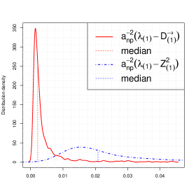
Figure 4. Density of the approximation errors for the eigenvalues of $a_{np}^{-2}{\mathbf{X}}{\mathbf{X}}^{\prime}$. The entries of ${\mathbf{X}}$ are iid with density (4.3) and $\alpha=1.6$.

According to the theory,

$$a_{np}^{-2}\sup_{i}|D_{(i)}^{\rightarrow}-\lambda_{(i)}|+a_{np}^{-2}\sup_{i}|Z^{2}_{(i),np}-\lambda_{(i)}|\stackrel{{\scriptstyle\mathbb{P}}}{{\rightarrow}}0\,,$$

but for finite $n$ the $(D_{(i)}^{\rightarrow})$ sequence yields a better approximation to $(\lambda_{(i)})$. By construction, the considered differences have a tendency to be positive but Figure 4 also shows that the median of the approximation error for $a_{np}^{-2}(\lambda_{(1)}-D_{(1)}^{\rightarrow})$ is almost zero.

Theorem 3.4 and the continuous mapping theorem immediately yield results about the joint convergence of the largest eigenvalues of the matrices $a_{np}^{-2}{\mathbf{X}}_{n}{\mathbf{X}}_{n}^{\prime}$ for $\alpha\in(0,2)$ and $\alpha\in(2,4)$ when $\beta$ satisfies $\widetilde{C}_{\beta}(\alpha)$. For fixed $k\geq 1$ one gets

$$a_{np}^{-2}\big{(}\lambda_{(1)},\ldots,\lambda_{(k)}\big{)}\stackrel{{\scriptstyle d}}{{\rightarrow}}\big{(}d_{(1)},\ldots,d_{(k)}\big{)}\,,$$

where $d_{(1)}\geq\cdots\geq d_{(k)}$ are the $k$ largest ordered values of the set $\{\Gamma_{i}^{-2/\alpha}v_{j},i=1,2,\ldots,j=1,\ldots,r\}$. The continuous mapping theorem yields for $k\geq 1$,

$$\dfrac{\lambda_{(1)}}{\lambda_{(1)}+\cdots+\lambda_{(k)}}\stackrel{{\scriptstyle d}}{{\rightarrow}}\dfrac{d_{(1)}}{d_{(1)}+\cdots+d_{(k)}}\,,\quad n\to\infty\,.$$ (4.4)

An application of the continuous mapping theorem to the distributional convergence of the point processes in Theorem 3.4 in the spirit of Resnick [29], Theorem 7.1, also yields the following result; see Davis et al. [11] for a proof and a similar result in the case $\alpha\in(2,4)$.

Corollary 4.2.

Assume the conditions of Theorem 3.1. If $\alpha\in(0,2]$ and $\mathbb{E}[Z^{2}]=\infty$, then

$$a_{np}^{-2}\Big{(}\lambda_{(1)},\sum_{i=1}^{p}\lambda_{i}\Big{)}\stackrel{{\scriptstyle d}}{{\rightarrow}}\Big{(}v_{1}\,\Gamma_{1}^{-2/\alpha}\,,\sum_{j=1}^{r}v_{j}\,\sum_{i=1}^{\infty}\Gamma_{i}^{-2/\alpha}\Big{)}\,,$$

where $\Gamma_{1}^{-2/\alpha}$ is Fréchet $\Phi_{\alpha/2}$-distributed. and $\sum_{i=1}^{\infty}\Gamma_{i}^{-2/\alpha}$ has the distribution of a positive $\alpha/2$-stable random variable. In particular,

$$\dfrac{\lambda_{(1)}}{\lambda_{1}+\cdots+\lambda_{p}}\stackrel{{\scriptstyle d}}{{\rightarrow}}\dfrac{v_{1}}{\sum_{j=1}^{r}v_{j}}\;\dfrac{\Gamma_{1}^{-2/\alpha}}{\sum_{i=1}^{\infty}\Gamma_{i}^{-2/\alpha}}\,,\quad n\to\infty\,.$$ (4.5)

Remark 4.3.

The ratio

$$\dfrac{\lambda_{(1)}+\cdots+\lambda_{(k)}}{\lambda_{1}+\cdots+\lambda_{p}},\qquad k\geq 1\,,$$

plays an important role in PCA. It reflects the proportion of the total variance in the data that we can explain by the first $k$ principal components. It follows from Corollary 4.2 that for fixed $k\geq 1$,

$$\dfrac{\lambda_{(1)}+\cdots\lambda_{(k)}}{\lambda_{1}+\cdots+\lambda_{p}}\stackrel{{\scriptstyle d}}{{\rightarrow}}\dfrac{d_{(1)}+\cdots+d_{(k)}}{d_{(1)}+d_{(2)}+\cdots}\,.$$

Unfortunately, the limiting variable does in general not have a clean form. An exception is the case when $r=1$; see Example 4.6. Also notice that the trace of ${\mathbf{X}}{\mathbf{X}}^{\prime}$ coincides with $\lambda_{1}+\cdots+\lambda_{p}$.

To illustrate the theory we consider a simple moving average example taken from Davis et al. [11].

Example 4.4.

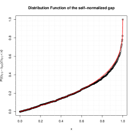
(a) iid data

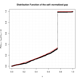
(b) data from model (4.6)

Figure 5. Distribution function of $(\lambda_{(1)}-\lambda_{(2)})/\lambda_{(1)}$ for iid data (left) and data generated from the model (4.6) (right). In each graph we compare the empirical distribution function (dotted line, based on 1000 simulations of $200\times 1000$ matrices with $Z$-distribution (4.3)) with the theoretical curve (solid line).

Assume that $\alpha\in(0,2)$ and

$$X_{it}=Z_{it}+Z_{i,t-1}-2(Z_{i-1,t}-Z_{i-1,t-1})\,,\quad i,t\in\mathbb{Z}\,.$$ (4.6)

In this case, the non-zero entries of ${\mathbf{H}}$ are

$$h_{00}=1,h_{01}=1,h_{10}=-2\quad\mbox{ and }\quad h_{11}=2.$$

Hence ${\mathbf{M}}={\mathbf{H}}{\mathbf{H}}^{\prime}$ has the positive eigenvalues $v_{1}=8$ and $v_{2}=2$. The limit point process in (3.17) is

$$N=\sum_{i=1}^{\infty}\varepsilon_{8\Gamma_{i}^{-2/\alpha}}+\sum_{i=1}^{\infty}\varepsilon_{2\Gamma_{i}^{-2/\alpha}}\,,$$

so that

$$a_{np}^{-2}\,\big{(}\lambda_{(1)},\lambda_{(2)}\big{)}\stackrel{{\scriptstyle d}}{{\rightarrow}}\big{(}8\Gamma_{1}^{-2/\alpha},2\Gamma_{1}^{-2/\alpha}\vee 8\Gamma_{2}^{-2/\alpha}\big{)}\,.$$

Using the fact that $U=\Gamma_{1}/\Gamma_{2}$ has a uniform distribution on $(0,1)$ we calculate

$$\mathbb{P}(2\Gamma_{1}^{-2/\alpha}>8\Gamma_{2}^{-2/\alpha})=\mathbb{P}(\Gamma_{1}/\Gamma_{2}<2^{-\alpha})=2^{-\alpha}\in(1/4,1).$$

In particular, we have for the normalized spectral gap

$$a_{np}^{-2}\big{(}\lambda_{(1)}-\lambda_{(2)}\big{)}\stackrel{{\scriptstyle d}}{{\rightarrow}}6\,\Gamma_{1}^{-2/\alpha}\mathbf{1}_{\{\Gamma_{1}4^{\alpha/2}<\Gamma_{2}\}}+8\,\big{(}\Gamma_{1}^{-2/\alpha}-\Gamma_{2}^{-2/\alpha}\big{)}\mathbf{1}_{\{\Gamma_{1}4^{\alpha/2}>\Gamma_{2}\}}$$

and for the self-normalized spectral gap (see also Example 4.5 for a detailed analysis)

$$\begin{split}\dfrac{\lambda_{(1)}-\lambda_{(2)}}{\lambda_{(1)}}&\stackrel{{\scriptstyle d}}{{\rightarrow}}\dfrac{6}{8}\,\mathbf{1}_{\{\Gamma_{1}2^{\alpha}<\Gamma_{2}\}}+\big{(}1-(\Gamma_{1}/\Gamma_{2})^{2/\alpha}\big{)}\mathbf{1}_{\{\Gamma_{1}2^{\alpha}>\Gamma_{2}\}}\\ &=\dfrac{3}{4}\,\mathbf{1}_{\{U2^{\alpha}<1\}}+\big{(}1-U^{2/\alpha}\big{)}\mathbf{1}_{\{U2^{\alpha}>1\}}=Y\,.\end{split}$$

The limit distribution of the spectral gap has an atom at $3/4$ with probability $2^{-\alpha}$, i.e., $\mathbb{P}(Y=3/4)=2^{-\alpha}$, and

$$\mathbb{P}(Y\leq x)=1-(1-x)^{\alpha/2},\qquad x\in(0,3/4).$$

In the iid case the limit distribution of the self-normalized spectral gap has distribution function $F(x)=1-(1-x)^{\alpha/2}$ for $x\in[0,1]$. This means that the atom disappears if the entries are iid. Figure 5 compares the distribution function of $Y$ with $F$ for $\alpha=0.6$; the atom at $3/4$ is clearly visible.

Along the same lines, we also have

$$(a_{np}^{-2}\lambda_{(1)},\lambda_{(2)}/\lambda_{(1)})\stackrel{{\scriptstyle d}}{{\rightarrow}}(8\,\Gamma_{1}^{-2/\alpha},\frac{1}{4}\,\mathbf{1}_{\{U<2^{-\alpha}\}}+U^{2/\alpha}\,\mathbf{1}_{\{U\geq 2^{-\alpha}\}})\,$$

and hence the limit distribution of $\lambda_{(2)}/\lambda_{(1)}$ is supported on $[1/4,1)$ with mass of $2^{-\alpha}$ at $1/4$. The histogram of the ratio $\left(\lambda_{(2)}/\lambda_{(1)}\right)^{2/\alpha}$ based on 1000 replications from the model (4.6) with noise given by a $t$-distribution with $\alpha=1.5$ degrees of freedom, $n=1000$ and $p=200$ is displayed in Figure 6.

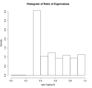
Figure 6. Histogram based on 1000 replications of $\left(\lambda_{(2)}/\lambda_{(1)}\right)^{2/\alpha}$ from model (4.6).

Observing that $2^{-\alpha}=0.3536\ldots$, the histogram is remarkably close to what one would expect from a sample from the truncated uniform distribution, $2^{-\alpha}\,\mathbf{1}_{\{U<2^{-\alpha}\}}+U\,\mathbf{1}_{\{U\geq 2^{-\alpha}\}}$. The mass of the limiting discrete component of the ratio can be much larger if one conditions on $a_{np}^{-2}\lambda_{(1)}$ being large. Specifically, for any $\epsilon\in(0,1/4)$ and $x>0$,

$$\lim_{n\to\infty}\mathbb{P}(\epsilon<\lambda_{(2)}/\lambda_{(1)}\leq 1/4|\lambda_{(1)}>a_{np}^{2}x)=\mathbb{P}(\Gamma_{1}/\Gamma_{2}\leq 2^{-\alpha}|\Gamma_{1}<(x/8)^{-\alpha/2})=G(x)\,.$$

The function $G$ approaches $1$ as $x\to\infty$ indicating the speed at which the two largest eigenvalues get linearly related; see Figure 7 for a graph of $G$ in the case $\alpha=1.5$.

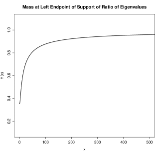
Figure 7. Graph of $G(x)=\mathbb{P}(\Gamma_{1}/\Gamma_{2}\leq 2^{-\alpha}|\Gamma_{1}<(x/8)^{-\alpha/2})$ when $\alpha=1.5$.

In addition, from Remark 4.3, we also have

$$\dfrac{\lambda_{(1)}}{\lambda_{1}+\cdots+\lambda_{p}}\stackrel{{\scriptstyle d}}{{\rightarrow}}\dfrac{4}{5}\,\dfrac{\Gamma_{1}^{-2/\alpha}}{\sum_{i=1}^{\infty}\Gamma_{i}^{-2/\alpha}}\,.$$

Clearly, the limit random variable is stochastically smaller than what one would get in the iid case; see (4.5).

Example 4.5.

The previous example also illustrates the behavior of the two largest eigenvalues in the general case when the rank $r$ of the matrix ${\mathbf{M}}$ is larger than one. We have in general

$$\dfrac{\lambda_{(2)}}{\lambda_{(1)}}\stackrel{{\scriptstyle d}}{{\rightarrow}}\frac{v_{2}}{v_{1}}\,\mathbf{1}_{\{U<(v_{2}/v_{1})^{\alpha/2}\}}+U^{2/\alpha}\,\mathbf{1}_{\{U\geq(v_{2}/v_{1})^{\alpha/2}\}}\,.$$

In particular, the limiting self-normalized spectral gap has representation

$$\dfrac{\lambda_{(1)}-\lambda_{(2)}}{\lambda_{(1)}}\stackrel{{\scriptstyle d}}{{\rightarrow}}\dfrac{v_{1}-v_{2}}{v_{1}}\,\mathbf{1}_{\{U<(v_{2}/v_{1})^{\alpha/2}\}}+(1-U^{2/\alpha})\,\mathbf{1}_{\{U\geq(v_{2}/v_{1})^{\alpha/2}\}}\,.$$

The limiting variable assumes values in $(0,1-v_{2}/v_{1}]$ and has an atom at the right end-point. This is in contrast to the iid case and to the case when $r=1$ (hence $v_{2}=0$) including the case of iid rows and the separable case; see Example 4.6.

Example 4.6.

We consider the separable case when $h_{kl}=\theta_{k}c_{l}$, $k,l\in\mathbb{Z}$, where $(c_{l})$, $(\theta_{k})$ are real sequences such that the conditions on $(h_{kl})$ in Theorem 3.1 hold. In this case,

$${\mathbf{M}}=\sum_{l\in\mathbb{Z}}c_{l}^{2}\;\;(\theta_{i}\theta_{j})_{i,j\in\mathbb{Z}}\,.$$

Note that $r=1$ with the only non-negative eigenvalue

$$v_{1}=\sum_{l\in\mathbb{Z}}c_{l}^{2}\;\;\sum_{k\in\mathbb{Z}}\theta_{k}^{2}\,.$$

In this case, the limiting point process in Theorem 3.4 is a PRM on $(0,\infty)$ with mean measure of $(y,\infty)$ given by $(v_{1}/y)^{\alpha/2}$, $y>0$. The normalized eigenvalues have similar asymptotic behavior as in the case of iid entries. For example, the log-spacings have the same limit as in the iid case for fixed $k$,

$$\big{(}\log\lambda_{(1)}-\log\lambda_{(2)},\ldots,\log\lambda_{(k+1)}-\log\lambda_{(k)}\big{)}\stackrel{{\scriptstyle\rm d}}{{\rightarrow}}-\dfrac{2}{\alpha}\,\big{(}\log(\Gamma_{1}/\Gamma_{2}),\ldots,\log(\Gamma_{k}/\Gamma_{k+1})\big{)}\,.$$

The same observation applies to the ratio of the largest eigenvalue and the trace in the case $\alpha\in(0,2)$:

$$\dfrac{\lambda_{(1)}}{{\rm tr}({\mathbf{X}}{\mathbf{X}}^{\prime})}=\dfrac{\lambda_{(1)}}{\lambda_{1}+\cdots+\lambda_{p}}\stackrel{{\scriptstyle\rm d}}{{\rightarrow}}\dfrac{\Gamma_{1}^{-2/\alpha}}{\sum_{i=1}^{\infty}\Gamma_{i}^{-2/\alpha}}\,.$$

We also mentioned in Example 4.5 that the distributional limit of the self-normalized spectral gap has no atom as in the iid case.

4.2. S&P 500 data

We conduct a short analysis of the largest eigenvalues of the univariate log-return time series which compose the S&P 500 stock index; see Section 1.2 for a description of the data. Although there is strong empirical evidence that these univariate series have power-law tails (see Figure 3) we do not expect that they have the same tail index. One way to proceed would be to ignore this fact because the tail indices are in a close range and the differences are due to large sampling errors for estimating such quantities. One could also collect time series with similar tail indices in the same group. In this case, the dimension $p$ decreases. This grouping would be a rather arbitrary classification method. We have chosen a third way: to use rank transforms. This approach has its merits because it aims at standardizing the tails but it also has a major disadvantage: one destroys the covariance structure underlying the data.

Given a $p\times n$ matrix $(R_{it})_{i=1,\cdots,p;t=1,\cdots,n}$, we construct a matrix ${\mathbf{X}}$ via the rank transforms

$$X_{it}=-\Big{[}\log\Big{(}\frac{1}{n+1}\sum_{\tau=1}^{n}\mathbf{1}_{\{R_{i\tau}\leq R_{it}\}}\Big{)}\Big{]}^{-1}\,,\qquad i=1,\ldots,p;t=1,\ldots,n\,.$$

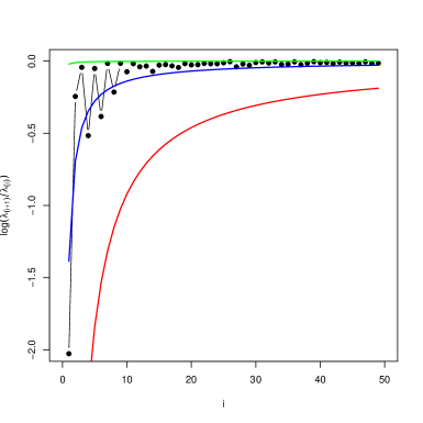
Figure 8. The logarithms of the ratios $\lambda_{(i+1)}/\lambda_{(i)}$ for the S&P 500 series after rank transform. We also show the 1, 50 and 99% quantiles (bottom, middle, top lines, respectively) of the variables $\log((\Gamma_{i}/\Gamma_{i+1})^{2})$.

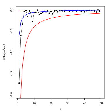
Figure 9. The logarithms of the ratios $\lambda_{(i+1)}/\lambda_{(i)}$ for the original (non-rank transformed) S&P 500 log-return data. We also show the 1, 50 and 99% quantiles (bottom, middle, top lines, respectively) of the variables $\log((\Gamma_{i}/\Gamma_{i+1})^{2/2.3})$; see also Figure 8 for comparison.

If the rows $R_{i1},\ldots,R_{in}$ were iid (or, more generally, stationary ergodic) with a continuous distribution  then the averages under the logarithm would be asymptotically uniform on $(0,1)$ as $n\to\infty$. Hence $X_{it}$ would be asymptotically standard Fréchet $\Phi_{1}$-distributed. In what follows, we assume that the aforementioned univariate time series of the S&P 500 index have undergone the rank transform and that their marginal distributions are close to $\Phi_{1}$; we always use the symbol ${\mathbf{X}}$ for the resulting multivariate series.

In Figure 8 we show the ratios of the consecutive ordered eigenvalues $(\lambda_{(i+1)}/\lambda_{(i)})$ of the matrix ${\mathbf{X}}{\mathbf{X}}^{\prime}$. This graph shows the rather surprising fact that the ratios are close to one even for small values $i$. We also show the 1, 50 and 99 % quantiles of the variables $((\Gamma_{i}/\Gamma_{i+1})^{2/\alpha})$ calculated from the formula

$$\mathbb{P}\big{(}(\Gamma_{i}/\Gamma_{i+1})^{2/\alpha}\leq x\big{)}=x^{i\cdot\alpha/2},\quad x\in(0,1)\,.$$ (4.7)

For increasing $i$, the distribution is concentrated closely to 1, in agreement with the strong law of large numbers which yields $\Gamma_{i}/\Gamma_{i+1}\stackrel{{\scriptstyle\rm a.s.}}{{\rightarrow}}1$ as $i\to\infty$. The asymptotic distributions (4.7) correspond to the case when the matrix ${\mathbf{M}}$ has rank $r=1$. It includes the iid and separable cases; see Example 4.6. The shown asymptotic quantiles are in agreement with the rank $r=1$ hypothesis.

For comparison, in Figure 9 we also show the ratios $(\lambda_{(i+1)}/\lambda_{(i)})$ for the non-rank transformed S&P 500 data and the 1, 50 and 99% quantiles of the variables $\log((\Gamma_{i}/\Gamma_{i+1})^{2/\alpha})$, where we choose $\alpha=2.3$ motivated by the estimated tail indices in Figure 3. The two graphs in Figure 8 and Figure 9 are quite similar but the smallest ratios for the original data are slightly larger than for the rank-transformed data.

4.3. Sums of squares of sample autocovariance matrices

In this section we consider some additive functions of the squares of ${\mathbf{A}}_{n}(s)={\mathbf{X}}_{n}(0){\mathbf{X}}_{n}(s)^{\prime}$ given by ${\mathbf{A}}_{n}(s){\mathbf{A}}_{n}(s)^{\prime}$ for $s=0,1,\ldots$. By definition of the singular values of a matrix (see (3.11)), the non-negative definite matrix ${\mathbf{A}}_{n}(s){\mathbf{A}}_{n}(s)^{\prime}$ has eigenvalues $(\lambda_{i}^{2}(s))_{i=1,\ldots,p}$.

The following result is a corollary of Theorem 3.1.

Proposition 4.7.

Consider the linear process (3.1) under the conditions of Theorem 3.1. Then the following statements hold for $s\geq 0$:

1. We consider two disjoint cases: $\alpha\in(0,2)$ and $\beta\in(0,\infty)$, or $\alpha\in[2,4)$ and $\beta$ satisfying $\widetilde{C}_{\beta}(\alpha)$. Then

   $$a_{np}^{-4}\max_{i=1,\ldots,p}|\lambda_{(i)}^{2}(s)-\delta_{(i)}^{2}(s)|\stackrel{{\scriptstyle\mathbb{P}}}{{\rightarrow}}0,\quad n\to\infty.$$

2. Assume $\beta\in[0,1]$. If $\alpha\in(0,2]$, $\mathbb{E}[Z^{2}]=\infty$ or $\alpha\in[2,4)$, $\mathbb{E}[Z^{2}]<\infty$ and $\beta\in(\alpha/2-1,1]$, then

   $$a_{np}^{-4}\max_{i=1,\ldots,p}|\lambda_{(i)}^{2}(s)-(\gamma_{(i)}^{\rightarrow}(s))^{2}|\stackrel{{\scriptstyle\mathbb{P}}}{{\rightarrow}}0,\quad n\to\infty.$$

   Assume $\beta>1$. If $\alpha\in(0,2]$, $\mathbb{E}[Z^{2}]=\infty$ or $\alpha\in[2,4)$, $\mathbb{E}[Z^{2}]<\infty$ and $\beta^{-1}\in(\alpha/2-1,1]$. Then

   $$a_{np}^{-4}\max_{i=1,\ldots,p}|\lambda_{(i)}^{2}(s)-(\gamma_{(i)}^{\downarrow}(s))^{2}|\stackrel{{\scriptstyle\mathbb{P}}}{{\rightarrow}}0,\quad n\to\infty.$$

To the best of our knowledge, sums of squares of sample autocovariance matrices were used first in the paper by Lam and Yao [26]; their time series model is quite different from ours.

Proof.

Part (1). The proof follows from Theorem 3.1 if we can show that

$$a_{np}^{-2}\max_{i=1,\ldots,p}\big{(}\lambda_{(i)}(s)+\delta_{(i)}(s)\big{)}=O_{\mathbb{P}}(1)\,\quad n\to\infty\,.$$

We have by Theorem 3.4,

$$a_{np}^{-2}\max_{i=1\ldots,p}\lambda_{(i)}(s)=a_{np}^{-2}\lambda_{(1)}(s)\stackrel{{\scriptstyle d}}{{\rightarrow}}c\,\xi_{\alpha/2}\,,$$ (4.8)

where $\xi_{\alpha/2}$ has a $\Phi_{\alpha/2}$ distribution. In view of Theorem 3.1(1) we also have

$$a_{np}^{-2}\max_{i=1\ldots,p}\delta_{(i)}(s)\stackrel{{\scriptstyle d}}{{\rightarrow}}c\,\xi_{\alpha/2}\,.$$

Therefore, again using Theorem 3.1(1), we have

$$a_{np}^{-4}\max_{i=1,\ldots,p}|\lambda_{(i)}^{2}(s)-\delta_{(i)}^{2}(s)|$$

$$\leq \big{[}a_{np}^{-2}\max_{i=1,\ldots,p}|\lambda_{(i)}(s)-\delta_{(i)}(s)|\big{]}\,\big{[}a_{np}^{-2}\max_{i=1,\ldots,p}\big{(}|\lambda_{(i)}(s)|+|\delta_{(i)}(s)|\big{)}\big{]}\stackrel{{\scriptstyle\mathbb{P}}}{{\rightarrow}}0,\quad n\to\infty.$$

This proves part (1).
Part (2). Now assume $\beta\in[0,1]$ and $\alpha\in(0,2]$, $\mathbb{E}[Z^{2}]=\infty$ or $\alpha\in[2,4)$, $\mathbb{E}[Z^{2}]<\infty$ and $\beta\in(\alpha/2-1,1]$. Then (4.8) is still true and we have by Theorem 3.1(2) and Theorem 3.4

$$a_{np}^{-2}\max_{i=1\ldots,p}\gamma_{(i)}^{\rightarrow}(s)\stackrel{{\scriptstyle d}}{{\rightarrow}}c\,\xi_{\alpha/2}\,.$$

We then have

$$a_{np}^{-4}\max_{i=1,\ldots,p}|\lambda_{(i)}^{2}(s)-(\gamma_{(i)}^{\rightarrow}(s))^{2}|$$

$$\leq \big{[}a_{np}^{-2}\max_{i=1,\ldots,p}|\lambda_{(i)}(s)-\gamma_{(i)}^{\rightarrow}(s)|\big{]}\,\big{[}a_{np}^{-2}\max_{i=1,\ldots,p}\big{(}\lambda_{(i)}(s)+\gamma_{(i)}^{\rightarrow}(s)\big{)}\big{]}\stackrel{{\scriptstyle\mathbb{P}}}{{\rightarrow}}0\,,\qquad n\to\infty.$$

The proof of the remaining part is similar and therefore omitted. ∎

Now, using Proposition 4.7 and a continuous mapping argument, we can show limit theory for the eigenvalues

$$w_{(1)}(s_{0},s_{1})\geq\cdots\geq w_{(p)}(s_{0},s_{1})\,,\qquad 0\leq s_{0}\leq s_{1}\,,$$

of the non-negative definite random matrices

$$\sum_{s=s_{0}}^{s_{1}}{\mathbf{A}}_{n}(s){\mathbf{A}}_{n}(s)^{\prime}\,.$$ (4.9)

Proposition 4.8.

Assume $0\leq s_{0}\leq s_{1}$ and the conditions of Theorem 3.1 hold. If $\alpha\in(0,4)$ and $\beta\in(0,1]\cap(\alpha/2-1,1]$ then

$$a_{np}^{-4}\max_{i=1,\ldots,p}|w_{(i)}(s_{0},s_{1})-\omega_{(i)}(s_{0},s_{1})|\stackrel{{\scriptstyle\mathbb{P}}}{{\rightarrow}}0,\quad n\to\infty,$$

where $\omega_{(i)}(s_{0},s_{1})$ are the ordered values of the set $\{Z_{(i),np}^{4}v_{j}(s_{0},s_{1}),i=1,\ldots,p;j=1,2,\ldots\}$ and $(v_{j}(s_{0},s_{1}))$ are the ordered eigenvalues of $\sum_{s=s_{0}}^{s_{1}}{\mathbf{M}}(s){\mathbf{M}}(s)^{\prime}$.

Example 4.9.

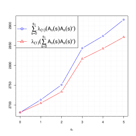
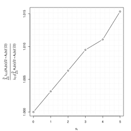
Figure 10. The largest eigenvalues of the sums of the squared autocovariance matrices compared with the sums of the largest eigenvalues of these matrices for the S&P 500 data for different values $s_{1}$. The two values are surprisingly close to each other; mind the scale of the $y$-axis. We also show their ratios.

Recall the separable case from Example 4.6, i.e., $h_{kl}=\theta_{k}c_{l}$, $k,l\geq 0$, where $(c_{l})$, $(\theta_{k})$ are real sequences such that the conditions on $(h_{kl})$ in Theorem 3.1 hold. Write $\Theta_{ij}=\theta_{i}\theta_{j}$. It is symmetric and has rank one; the only non-zero eigenvalue is $\gamma_{\theta}(0)=\sum_{k=0}^{\infty}\theta_{k}^{2}$. Hence $\Theta$ is non-negative definite. We get from (3.12) that

$${\mathbf{M}}(s)=\gamma_{c}(s)\,\Theta,\quad s\geq 0\,,$$

where

$$\gamma_{c}(s)=\sum_{l=0}^{\infty}c_{l}c_{l+s}\,,\qquad s\geq 0\,.$$

The matrix ${\mathbf{M}}(s)$ has the only non-zero eigenvalue $\gamma_{c}(s)\gamma_{\theta}(0)$. The factors $(\gamma_{c}(s))$ can be positive or negative; they constitute the autocovariance function of a stationary linear process with coefficients $(c_{l})$. Accordingly, ${\mathbf{M}}(s)$ is either non-negative or non-positive definite. Now we consider the non-negative definite matrix

$$\sum_{s=s_{0}}^{s_{1}}{\mathbf{M}}(s)\,{\mathbf{M}}(s)^{\prime}=\sum_{s=s_{0}}^{s_{1}}\gamma_{c}^{2}(s)\,\Theta\Theta^{\prime}\,.$$

This matrix has rank $1$ and its largest eigenvalue is given by

$$C_{c,\theta}(s_{0},s_{1})=\sum_{s=s_{0}}^{s_{1}}\gamma_{c}^{2}(s)\,\gamma_{\theta}^{2}(0)\,.$$

An application of Proposition 4.8 yields that the ordered eigenvalues of $a_{np}^{-4}\sum_{s=s_{0}}^{s_{1}}{\mathbf{A}}_{n}(s){\mathbf{A}}_{n}(s)^{\prime}$ are uniformly approximated by the quantities

$$a_{np}^{-4}Z_{(i),np}^{4}C_{c,\theta}(s_{0},s_{1})\,,\qquad i=1,\ldots,p\,.$$ (4.10)

Since

$$C_{c,\theta}(s_{0},s_{1})=\sum_{i=s_{0}}^{s_{1}}C_{c,\theta}(i,i)$$

one gets the remarkable property that

$$a_{np}^{-4}\max_{i=1,\ldots,p}\Big{|}\lambda_{(i)}\Big{(}\sum_{s=s_{0}}^{s_{1}}{\mathbf{A}}_{n}(s){\mathbf{A}}_{n}(s)^{\prime}\Big{)}-Z_{(i),np}^{4}C_{c,\theta}(s_{0},s_{1})\Big{|}$$

$$= a_{np}^{-4}\max_{i=1,\ldots,p}\Big{|}\sum_{s=s_{0}}^{s_{1}}\lambda_{(i)}({\mathbf{A}}_{n}(s){\mathbf{A}}_{n}(s)^{\prime})-Z_{(i),np}^{4}C_{c,\theta}(s_{0},s_{1})\Big{|}+o_{P}(1)\,.$$

In particular, for $s_{1}\geq s_{0}$ we get the weak convergence of the point processes towards a PRM:

$$\sum_{i=1}^{p}\varepsilon_{a_{np}^{-4}\Big{(}\lambda_{i}\Big{(}\sum_{s=s_{0}}^{s_{0}}{\mathbf{A}}_{n}(s){\mathbf{A}}_{n}(s)^{\prime}\big{)}\,,\ldots,\lambda_{i}\big{(}\sum_{s=s_{0}}^{s_{1}}{\mathbf{A}}_{n}(s){\mathbf{A}}_{n}(s)^{\prime}\big{)}\Big{)}}\stackrel{{\scriptstyle\rm d}}{{\rightarrow}}\sum_{i=1}^{\infty}\varepsilon_{\Gamma_{i}^{-4/\alpha}\Big{(}C_{c,\theta}(s_{0},s_{0}),\ldots,C_{c,\theta}(s_{0},s_{1})\Big{)}}\,.$$

Example 4.10.

In Figure 10 we calculate the largest eigenvalues $\lambda_{(1)}\big{(}\sum_{s=0}^{s_{1}}{\mathbf{A}}_{n}(s){\mathbf{A}}_{n}(s)^{\prime}\big{)}$ for $s_{1}=0,\ldots,5$ as well as the sums of the largest eigenvalues $\sum_{s=0}^{s_{1}}\lambda_{(1)}\big{(}{\mathbf{A}}_{n}(s){\mathbf{A}}_{n}(s)^{\prime}\big{)}$ the log-return series from the S&P 500 index described in Section 1.2. The data are not rank-transformed. We notice that the two values are surprisingly close across the values $s_{0}=0,\ldots,5$. This phenomenon could be explained by the structure of the eigenvalues in Example 4.9. Also note that the largest eigenvalue ${\mathbf{A}}_{n}(0){\mathbf{A}}_{n}(0)^{\prime}$ makes a major contribution to the values in Figure 10; the contribution of the squares ${\mathbf{A}}_{n}(s){\mathbf{A}}_{n}(s)^{\prime}$, $s=1,\ldots,5,$ to the largest eigenvalue of the sum of squares is less substantial.

Appendix A Auxiliary results

Let $(Z_{i})$ be iid copies of $Z$ whose distribution satisfies

$$\mathbb{P}(Z>x)\sim p_{+}\dfrac{L(x)}{x^{\alpha}}\quad\mbox{and}\quad\mathbb{P}(Z\leq-x)\sim p_{-}\dfrac{L(x)}{x^{\alpha}}\,,\quad x\to\infty\,,$$

for some tail index $\alpha>0$, where $p_{+},p_{-}\geq 0$ with $p_{+}+p_{-}=1$ and $L$ is a slowly varying function. If $\mathbb{E}[|Z|]<\infty$ also assume $\mathbb{E}[Z]=0$. The product $Z_{1}Z_{2}$ is regular varying with the same index $\alpha$ and $\mathbb{P}(|Z_{1}Z_{2}|>x)=x^{-\alpha}L_{1}(x)$, where $L_{1}$ is slowly varying function different from $L$; see Embrechts and Goldie [16]. Write

$$S_{n}=Z_{1}+\cdots+Z_{n}\,,\quad n\geq 1,$$

and consider a sequence $(a_{n})$ such that $\mathbb{P}(|Z|>a_{n})\sim n^{-1}$.

A.1. Large deviation results

The following theorem can be found in Nagaev [28] and Cline and Hsing [10] for $\alpha>2$ and $\alpha\leq 2$, respectively; see also Denisov et al. [14].

Theorem A.1.

Under the assumptions on the iid sequence $(Z_{t})$ given above the following relation holds

$$\sup_{x\geq c_{n}}\left|\dfrac{\mathbb{P}(S_{n}>x)}{n\mathbb{P}(|Z|>x)}-p_{+}\right|\to 0\,,$$

where $(c_{n})$ is any sequence satisfying $c_{n}/a_{n}\to\infty$ for $\alpha\leq 2$ and $c_{n}\geq\sqrt{(\alpha-2)n\log n}$ for $\alpha>2$.

A.2. A point process convergence result

Assume that the conditions at the beginning of Appendix A hold. Consider a sequence of iid copies $(S_{n}^{(t)})_{t=1,2,\ldots}$ of $S_{n}$ and the sequence of point processes

$$N_{n}=\sum_{t=1}^{p}\varepsilon_{a_{np}^{-1}S_{n}^{(t)}},\quad n=1,2,\ldots\,,$$

for an integer sequence $p=p_{n}\to\infty$. We assume that the state space of the point processes $N_{n}$ is $\overline{\mathbb{R}}_{0}=[\mathbb{R}\cup\{\pm\infty\}]\backslash\{0\}$.

Lemma A.2.

Assume $\alpha\in(0,2)$ and the conditions of Appendix A on the iid sequence $(Z_{t})$ and the normalizing sequence $(a_{n})$. Then the limit relation $N_{n}\stackrel{{\scriptstyle d}}{{\rightarrow}}N$ holds in the space of point measures on $\overline{\mathbb{R}}_{0}$ equipped with the vague topology (see [30, 29]) for a Poisson random measure $N$ with state space $\overline{\mathbb{R}}_{0}$ and intensity measure $\mu_{\alpha}(dx)=\alpha|x|^{-\alpha-1}(p_{+}\mathbf{1}_{\{x>0\}}+p_{-}\mathbf{1}_{\{x<0\}})dx$.

Proof.

According to Resnick [30], Proposition 3.21, we need to show that $p\,\mathbb{P}(a_{np}^{-1}S_{n}\in\cdot)\stackrel{{\scriptstyle v}}{{\rightarrow}}\mu_{\alpha}$, where $\stackrel{{\scriptstyle v}}{{\rightarrow}}$ denotes vague convergence of Radon measures on $\overline{\mathbb{R}}_{0}$. Observe that we have $a_{np}/a_{n}\to\infty$ as $n\to\infty$. This fact and $\alpha\in(0,2)$ allow one to apply Theorem A.1:

$$\dfrac{\mathbb{P}(S_{n}>xa_{np})}{n\,\mathbb{P}(|Z|>a_{np})}\to p_{+}x^{-\alpha}\quad\mbox{and}\quad\dfrac{\mathbb{P}(S_{n}\leq-xa_{np})}{n\,\mathbb{P}(|Z|>a_{np})}\to p_{-}\,x^{-\alpha}\,,\quad x>0\,.$$

On the other hand, $n\,\mathbb{P}(|Z|>a_{np})\sim p^{-1}$ as $n\to\infty$. This proves the lemma. ∎

References

- [1] Anderson, T. W. Asymptotic theory for principal component analysis. Ann. Math. Statist. 34 (1963), 122–148.
- [2] Auffinger, A., Ben Arous, G., and Péché, S. Poisson convergence for the largest eigenvalues of heavy tailed random matrices. Ann. Inst. Henri Poincaré Probab. Stat. 45, 3 (2009), 589–610.
- [3] Bai, Z., and Silverstein, J. W. Spectral Analysis of Large Dimensional Random Matrices, second ed. Springer Series in Statistics. Springer, New York, 2010.
- [4] Bai, Z. D., Silverstein, J. W., and Yin, Y. Q. A note on the largest eigenvalue of a large-dimensional sample covariance matrix. J. Multivariate Anal. 26, 2 (1988), 166–168.
- [5] Belinschi, S., Dembo, A., and Guionnet, A. Spectral measure of heavy tailed band and covariance random matrices. Comm. Math. Phys. 289, 3 (2009), 1023–1055.
- [6] Belitskiĭ, G. R., and Lyubich, Y. I. Matrix Norms and their Applications, vol. 36 of Operator Theory: Advances and Applications. Birkhäuser Verlag, Basel, 1988.
- [7] Ben Arous, G., and Guionnet, A. The spectrum of heavy tailed random matrices. Comm. Math. Phys. 278, 3 (2008), 715–751.
- [8] Bhatia, R. Matrix Analysis, vol. 169 of Graduate Texts in Mathematics. Springer-Verlag, New York, 1997.
- [9] Bingham, N. H., Goldie, C. M., and Teugels, J. L. Regular Variation, vol. 27 of Encyclopedia of Mathematics and its Applications. Cambridge University Press, Cambridge, 1987.
- [10] Cline, D. B. H., and Hsing, T. Large deviation probabilities for sums of random variables with heavy or subexponential tails. Technical report. Statistics Dept., Texas A&M University. (1998).
- [11] Davis, R. A., Mikosch, T., and Pfaffel, O. Asymptotic theory for the sample covariance matrix of a heavy-tailed multivariate time series. Stochastic Process. Appl. (2015).
- [12] Davis, R. A., Pfaffel, O., and Stelzer, R. Limit theory for the largest eigenvalues of sample covariance matrices with heavy-tails. Stochastic Process. Appl. 124, 1 (2014), 18–50.
- [13] de Haan, L., and Ferreira, A. Extreme Value Theory: An Introduction. Springer Series in Operations Research and Financial Engineering. Springer, New York, 2006.
- [14] Denisov, D., Dieker, A. B., and Shneer, V. Large deviations for random walks under subexponentiality: the big-jump domain. Ann. Probab. 36, 5 (2008), 1946–1991.
- [15] El Karoui, N. On the largest eigenvalue of wishart matrices with identity covariance when n,p and p/n tend to infinity. Available at http://arxiv.org/abs/math/0309355 (2003).
- [16] Embrechts, P., and Goldie, C. M. On closure and factorization properties of subexponential and related distributions. J. Austral. Math. Soc. Ser. A 29, 2 (1980), 243–256.
- [17] Embrechts, P., Klüppelberg, C., and Mikosch, T. Modelling Extremal Events for Insurance and Finance, vol. 33 of Applications of Mathematics (New York). Springer, Berlin, 1997.
- [18] Embrechts, P., and Veraverbeke, N. Estimates for the probability of ruin with special emphasis on the possibility of large claims. Insurance Math. Econom. 1, 1 (1982), 55–72.
- [19] Feller, W. An Introduction to Probability Theory and its Applications. Vol. II. John Wiley & Sons, Inc., New York-London-Sydney, 1966.
- [20] Geman, S. A limit theorem for the norm of random matrices. Ann. Probab. 8, 2 (1980), 252–261.
- [21] Heiny, J., and Mikosch, T. Eigenvalues and eigenvectors of heavy-tailed sample covariance matrices with general growth rates: the iid case. Submitted (2015).
- [22] Heiny, J., Mikosch, T., and Davis, R. A. Limit theory for the singular values of the sample autocovariance matrix function of multivariate time series. Work in progress (2015).
- [23] Horn, R. A., and Johnson, C. R. Matrix Analysis, second ed. Cambridge University Press, Cambridge, 2013.
- [24] Johansson, K. Universality of the local spacing distribution in certain ensembles of Hermitian Wigner matrices. Comm. Math. Phys. 215, 3 (2001), 683–705.
- [25] Johnstone, I. M. On the distribution of the largest eigenvalue in principal components analysis. Ann. Statist. 29, 2 (2001), 295–327.
- [26] Lam, C., and Yao, Q. Factor modeling for high-dimensional time series: inference for the number of factors. Ann. Statist. 40, 2 (2012), 694–726.
- [27] Muirhead, R. J. Aspects of Multivariate Statistical Theory. John Wiley & Sons, Inc., New York, 1982. Wiley Series in Probability and Mathematical Statistics.
- [28] Nagaev, S. V. Large deviations of sums of independent random variables. Ann. Probab. 7, 5 (1979), 745–789.
- [29] Resnick, S. I. Heavy-Tail Phenomena: Probabilistic and Statistical Modeling. Springer Series in Operations Research and Financial Engineering. Springer, New York, 2007.
- [30] Resnick, S. I. Extreme Values, Regular Variation and Point Processes. Springer Series in Operations Research and Financial Engineering. Springer, New York, 2008. Reprint of the 1987 original.
- [31] Shores, T. S. Applied Linear Algebra and Matrix Analysis. Undergraduate Texts in Mathematics. Springer, New York, 2007.
- [32] Soshnikov, A. Poisson statistics for the largest eigenvalues of Wigner random matrices with heavy tails. Electron. Comm. Probab. 9 (2004), 82–91 (electronic).
- [33] Soshnikov, A. Poisson statistics for the largest eigenvalues in random matrix ensembles. In Mathematical physics of quantum mechanics, vol. 690 of Lecture Notes in Phys. Springer, Berlin, 2006, pp. 351–364.
- [34] Tao, T., and Vu, V. Random matrices: universality of local eigenvalue statistics up to the edge. Comm. Math. Phys. 298, 2 (2010), 549–572.
- [35] Tracy, C. A., and Widom, H. Distribution functions for largest eigenvalues and their applications. In Proceedings of the International Congress of Mathematicians, Vol. I (Beijing, 2002) (2002), Higher Ed. Press, Beijing, pp. 587–596.