Relativistic stars in scalar-tensor theories with disformal coupling
Abstract
We present a general formulation to analyze the structure of slowly rotating relativistic stars in a broad class of scalar-tensor theories with disformal coupling to matter. Our approach includes theories with generalized kinetic terms, generic scalar field potentials and contains theories with conformal coupling as particular limits. In order to investigate how the disformal coupling affects the structure of relativistic stars, we propose a minimal model of a massless scalar-tensor theory and investigate in detail how the disformal coupling affects the spontaneous scalarization of slowly rotating neutron stars. We show that for negative values of the disformal coupling parameter between the scalar field and matter, scalarization can be suppressed, while for large positive values of the disformal coupling parameter stellar models cannot be obtained. This allows us to put a mild upper bound on this parameter. We also show that these properties can be qualitatively understood by linearizing the scalar field equation of motion in the background of a general-relativistic incompressible star. To address the intrinsic degeneracy between uncertainties in the equation-of-state of neutron stars and gravitational theory, we also show the existence of universal equation-of-state-independent relations between the moment of inertia and compactness of neutron stars in this theory. We show that in a certain range of the theory’s parameter space the universal relation largely deviates from that of general relativity, allowing, in principle, to probe the existence of spontaneous scalarization with future observations.
pacs:
04.40.Dg, 97.60.Jd, 04.50.Kd, 04.80.CcI Introduction
Although Einstein’s general relativity (GR) has passed all the experimental tests of gravity in the weak-field/slow-motion regimes with flying colors Will (2014), it remains fairly unconstrained in the strong-gravity regime Berti et al. (2015) and on the cosmological scales Clifton et al. (2012). The recent observation of gravitational waves generated during the merger of two black holes (BHs) by the LIGO/Virgo Collaboration, in accordance with general-relativistic predictions Abbott et al. (2016a, b), has offered us a first glimpse of gravity in a fully nonlinear and highly dynamical regime whose theoretical implications are still being explored Yunes et al. (2016). Nevertheless, the pressing issues on understanding the nature of dark matter and dark energy, the inflationary evolution of the early Universe and the quest for an ultraviolet completion of GR have served as driving forces in the exploration of modifications to GR Clifton et al. (2012); Berti et al. (2015).
In general modifications of GR introduce new gravitational degree(s) of freedom in addition to the metric tensor and can be described by a scalar-tensor theory of gravity Fujii and Maeda (2003). On the theoretical side, scalar-tensor theories should not contain Ostrogradski ghosts Woodard (2015), i.e. the equations of motion should be written in terms of the second-order differential equations despite the possible existence of the higher-order derivative interactions at the action level. On the experimental/observational side, any extension of GR must pass all the current weak-field tests which GR has successfully passed. Therefore realistic modifications of gravity should contain a mechanism to suppress scalar interactions at small scales Vainshtein (1972); Brax et al. (2004) or (to be interesting) satisfy weak-field tests, but deviate from GR at some energy scale. Some models satisfying these requirements belongs to the so-called Horndeski theory Horndeski (1974); Deffayet et al. (2009a, 2011); Kobayashi et al. (2011), the most general scalar-tensor theory with second-order equations of motion.
In scalar-tensor theories, the scalar field may directly couple to matter, and hence matter does not follow geodesics associated with the metric but with another . In the simplest case these two metrics are related as
| (1) |
which is known as the conformal coupling Clifton et al. (2012). The two frames described by and are often referred to as the Einstein and Jordan frames, respectively.
I.1 Spontaneous scalarization
For relativistic stars, such as neutron stars (NSs), the conformal coupling to matter can trigger a tachyonic instability (due to a negative effective mass) of the scalar field when the star has a compactness above a certain threshold. This instability spontaneously scalarizes the NS, whereupon it harbors a nontrivial scalar field configuration which smoothly decays outside the star. In its simplest realization, scalarization occurs when the conformal factor in Eq. (1) is chosen as , where is a free parameter of the theory and is a massless scalar field. This theory passes all weak-field tests, but the presence of the scalar field can significantly modify the bulk properties of NSs, such as masses and radii, in comparison with GR. This effect was first analyzed for isolated NSs by Damour and Esposito-Farèse Damour and Esposito-Farèse (1993, 1996a). The properties and observational consequences of this phenomenon were studied in a number of situations, including stability Harada (1997); Chiba et al. (1997), asteroseismology Sotani and Kokkotas (2004, 2005); Sotani (2014); Silva et al. (2014), slow (and rapidly) rotating NS solutions Damour and Esposito-Farèse (1996a); Sotani (2012); Doneva et al. (2013, 2014a); Pani and Berti (2014), its influence on geodesic motion of particles around NSs DeDeo and Psaltis (2004); Doneva et al. (2014b), tidal interactions Pani and Berti (2014) and the multipolar structure of the spacetime Pappas and Sotiriou (2015a, b). Moreover, the dynamical process of scalarization was studied in Ref. Novak (1998a) and stellar collapse (including the associated process of scalar radiation emission) was investigated in Refs. Harada et al. (1997); Novak (1998b); Gerosa et al. (2016). We refer the reader to Ref. Horbatsch and Burgess (2011) for an extensive literature review.
Additionally, a semiclassical version of this effect Lima et al. (2010) (cf. also Landulfo et al. (2012); Mendes et al. (2014a); Landulfo et al. (2015); Mendes et al. (2014b) and Pani et al. (2011) for a connection with the Damour-Esposito-Farèse model Damour and Esposito-Farèse (1993, 1996a)) has been shown to awaken the vacuum state of a quantum field leading to an exponential growth of its vacuum energy density in the background of a relativistic star.
These nontrivial excitations of scalar fields induced by relativistic stars are a consequence of the generic absence of a “no-hair theorem” for these objects (see Refs. Yagi et al. (2012, 2016); Barausse and Yagi (2015) for counterexamples), in contrast to the case of BHs, and can potentially be an important source for signatures of the presence of fundamental gravitational scalar degrees of freedom through astronomical observations Psaltis (2008); Berti et al. (2015), including the measurements of gravitational and scalar radiation signals Yunes and Siemens (2013).
The phenomenological implications of spontaneous scalarization have also been explored in binary NS mergers Barausse et al. (2013); Palenzuela et al. (2014); Taniguchi et al. (2015); Sennett and Buonanno (2016) and in BHs surrounded by matter Cardoso et al. (2013a, b). In the former situation, a dynamical scalarization allows binary members to scalarize under conditions where this would not happen if they were isolated. This effect can dramatically change the dynamics of the system in the final cycles before the merger with potentially observable consequences. In the latter case, the presence of matter can cause the appearance of a nontrivial scalar field configuration, growing “hair” on the BH.
On the experimental side, binary-pulsar observations Freire et al. (2012) have set stringent bounds on , whose value is presently constrained to be . This tightly constrains the effects of spontaneous scalarization in isolated NSs, for it has been shown that independently of the choice of the equation of state (EOS) scalarization can occur only if for NSs modeled by a perfect fluid Harada (1998); Novak (1998a); Silva et al. (2015). These two results confine to a very limited range, in which, even if it exists in nature, the effects of scalarization on isolated NSs are bound to be small; see Refs. Silva et al. (2015); Doneva et al. (2013) for examples where the threshold value of can be increased and Refs. Mendes (2015); Palenzuela and Liebling (2016); Mendes and Ortiz (2016) for recent work exploring the large positive region of the theory.
I.2 Disformal coupling
It was recently understood that modern scalar-tensor theories of gravity, under the umbrella of Horndeski gravity Horndeski (1974); Deffayet et al. (2009b), offer a more general class of coupling Bettoni and Liberati (2013); Zumalacárregui and García-Bellido (2014) between the scalar field and matter through the so-called disformal coupling Bekenstein (1993)
| (2) |
where is the covariant derivative of the scalar field associated with the gravity frame metric , and is a constant with dimensions of . For we recover the purely conformal case of Eq. (1). Disformal transformations were originally introduced by Bekenstein and consist of the most general coupling constructed from the metric and the scalar field that respects causality and the weak equivalence principle Bekenstein (1993). Disformal couplings have been investigated so far mainly in the context of cosmology Koivisto (2008); Sakstein (2015); Sakstein and Verner (2015). They also arise in higher-dimensional gravitational theories with moving branes Zumalacarregui et al. (2013); Koivisto et al. (2014) in relativistic extensions of modified Newtonian theories, the tensor-vector-scalar theories Bekenstein (2004); Bekenstein and Sanders (1994), and in the decoupling limit of the nonlinear massive gravity de Rham et al. (2011); de Rham and Gabadadze (2010); Berezhiani et al. (2013); Brito et al. (2014). Moreover, in Ref. Bettoni and Liberati (2013) it was shown that the mathematical structure of Horndeski theory is preserved under the transformation (2), namely if the scalar-tensor theory written in terms of belongs to a class of the Horndeski theory the same theory rewritten in terms of belongs to another class of the Horndeski theory. Thus disformal transformations provide a natural generalization of conformal transformations.
Disformal coupling was also considered in models of a varying speed of light Magueijo (2003) and inflation Kaloper (2004); van de Bruck et al. (2016). The invariance of cosmological observables in the frames related by the disformal relation (2) was verified in Refs. Creminelli et al. (2014); Minamitsuji (2014); Tsujikawa (2015); Watanabe et al. (2015); Motohashi and White (2016); Domenech et al. (2015). Although applications to early Universe models are still limited, disformal couplings have been extensively applied to late-time cosmology Sakstein (2014); van de Bruck and Morrice (2015); Sakstein and Verner (2015); Koivisto (2008); Zumalacarregui et al. (2013, 2010); Koivisto et al. (2012); De Felice and Tsujikawa (2012); Bettoni et al. (2012); Hagala et al. (2016). A new screening mechanism of the scalar force in the high-density region was proposed in Ref. Koivisto et al. (2012), where in the presence of disformal coupling the nonrelativistic limit of the scalar field equation seemed to be independent of the local energy density. However, a reanalysis suggested that no new screening mechanism from disformal coupling could work Sakstein (2014); Ip et al. (2015). It was also argued that disformal coupling could not contribute to a chameleon screening mechanism around a nonrelativistic source Noller (2012). Experimental and observational constraints on disformal coupling to particular matter sectors have also been investigated. Disformal couplings to baryons and photons have been severely constrained in terms of the nondetection of new physics in collider experiments Kaloper (2004); Brax and Burrage (2014, 2015); Brax et al. (2015a); Lamm (2015); Brax et al. (2015b), the absence of spectral distortion of the cosmic microwave background and the violation of distance reciprocal relations van de Bruck et al. (2013); Brax et al. (2013, 2015a); van de Bruck et al. (2015), respectively. On the other hand, disformal coupling to the dark sector has been proposed in Neveu et al. (2014); van de Bruck and Morrice (2015) and is presently less constrained in comparison with coupling to visible matter sectors.
When conformal and disformal couplings are universal to all the matter species, they can only be constrained through experimental tests of gravity. A detailed study of scalar-tensor theory with the pure disformal coupling and in the weak-field limit was presented in Sakstein (2014) and the post-Newtonian (PN) corrections due to the presence of pure disformal coupling were computed Ip et al. (2015). In these papers Sakstein (2014); Ip et al. (2015), in contrast to the claim of Refs. Zumalacarregui et al. (2013); Koivisto et al. (2012), it was shown that no screening mechanism which could suppress the scalar force in the vicinity of the source exists and the difference of the parametrized post-Newtonian (PPN) parameters from GR are of order , where is the present-day Hubble scale. The strongest bound on comes from the constraints on the PPN preferred frame parameter . The near perfect alignment between the Sun’s spin axis and the orbital angular momenta of the planets provides the constraint (see Ref. Iorio (2014) for a discussion), which implies that . With the inclusion of the conformal factor, i.e. , the authors of Ref. Ip et al. (2015) argued that the Cassini bound Bertotti et al. (2003) imposes a constraint on , where is the cosmological background value of the scalar field and
| (3) |
On the other hand the disformal part of the coupling remains unconstrained, because corrections to the PPN parameters which include are subdominant compared to the conformal part. These weaker constraints on the disformal coupling parameters are due to the fact that in the nonrelativistic regime with negligible pressure and a slowly evolving scalar field the disformal coupling becomes negligible. We also point out that in the weak-field regime such as in the Solar System, typical densities are small therefore preventing the appearance of ghosts in the theory for negative values of .
In the strong-gravity regime such as that found in the interior of NSs, the pressure cannot be neglected and the disformal coupling is expected to be as important as the conformal one. This would affect the spontaneous scalarization mechanism and consequently influence the structure (and stability) of relativistic stars, or have significant impact on gravitational-wave astronomy Berti et al. (2015). The influence of disformal coupling on the stability of matter configurations around BHs was analyzed in Ref. Koivisto and Nyrhinen (2015). The authors of Ref. Koivisto and Nyrhinen (2015) derived the stability conditions of the system by generalizing the case of pure conformal coupling Cardoso et al. (2013a, b). They also generalized these works to scalar-tensor theories with noncanonical kinetic terms and disformal coupling, finding that the disformal coupling could make matter configurations more unstable, triggering spontaneous scalarization. In the present work within the same class of scalar-tensor theory considered in Ref. Koivisto and Nyrhinen (2015), we will study relativistic stars and investigate the influence of disformal coupling on the scalarization of NSs.
I.3 Organization of this work
This paper is organized as follows. In Sec. II we review the fundamentals of scalar-tensor theories with generalized kinetic term and disformal coupling. In Sec. III we present a general formulation to analyze the structure of slowly rotating stars in theories with disformal coupling. In Sec. IV, as a case study, we consider a canonical scalar field with a generic scalar field potential. We particularize the stellar structure equations to this model and discuss how to solve them numerically. In Sec. V we explore the consequences of the disformal coupling by studying small scalar perturbations to an incompressible relativistic star in GR. In particular we investigate the conditions for which spontaneous scalarization happens. In Sec. VI we present our numerical studies about the influence of disformal coupling on the spontaneous scalarization by solving the full stellar structure equations. In Sec. VII as an application of our numerical integrations, we examine the EOS independence between the moment of inertia and compactness of NSs in scalar-tensor theory comparing it against the results obtained in GR. Finally, in Sec. VIII we summarize our main findings and point out possible future avenues of research.
II Scalar-tensor theory with the disformal coupling
We consider scalar-tensor theories in which matter is disformally coupled to the scalar field. The action in the Einstein frame reads
| (4) |
where () represents the coordinate system of the spacetime, and are respectively the Einstein and Jordan frame metrics disformally related by (2), and , is the Ricci scalar curvature associated with , , where is the gravitational constant defined in the Einstein frame and is the speed of light in vacuum. is an arbitrary function of the scalar field and , and represents the Lagrangian density of matter fields . We note that the canonical scalar field corresponds to the case of , but we will not restrict the form of at this stage. In this paper we will not omit and .
Varying the action (4) with respect to the Einstein frame metric , we obtain the Einstein field equations
| (5) |
where the energy-momentum tensors of the matter fields and scalar field are given by
| (6) |
and
| (7) |
respectively, where and . From Eq. (2), the inverse Jordan frame metric is related to the inverse Einstein frame metric by
| (8) |
where we have defined
| (9) |
The volume element in the Jordan frame is given by . In order to keep the Lorentzian signature of the Jordan frame metric , must be non-negative. We note that in the purely conformal coupling limit and .
The contravariant energy-momentum tensor in the Jordan frame is related to that in the Einstein frame by
| (10) |
The mixed and covariant energy-momentum tensors in the Jordan frame are respectively given by
| (11a) | ||||
| (11b) | ||||
and
| (12a) | ||||
| (12b) | ||||
| (12c) | ||||
In terms of the covariant tensors, the Einstein equations in the Einstein frame (5) can be recast as
| (13) |
Varying the action (4) with respect to the scalar field , we obtain the scalar field equation of motion
| (14) |
where the function characterizes the strength of the coupling of matter to the scalar field
| (15) |
where is the trace of , and and were defined in Eq. (3). Taking the divergence of Eq. (5), employing the contracted Bianchi identity , and using the scalar field equation of motion (14), we obtain
| (16) |
and the coupling strength can be rewritten as
| (17) |
where we have introduced
| (18) |
Multiplying Eq. (16) by and solving it with respect to , we obtain
| (19) |
Then, substituting it in Eq. (17), using , and finally eliminating from Eq. (14), we obtain the reduced scalar field equation of motion
| (20) |
III The equations of stellar structure
III.1 Equations of motion
In this section, we consider a static and spherically symmetric spacetime with line element
| (21) |
where and are functions of the radial coordinate only, is the metric of the unit 2-sphere, and the coordinates () run over the directions of the unit 2-sphere, such that . We also assume by symmetry that the scalar field is only a function of , . Hence the coupling functions and are also only functions of through .
We assume that in the Jordan frame only diagonal components of the energy-momentum tensor of matter are nonvanishing
| (22) |
where , and are respectively the energy density, radial and tangential pressures of an anisotropic fluid in the Jordan frame Bowers and Liang (1974). Using Eq. (12b), they are related to the components of the energy-momentum tensor of matter in the Einstein frame, which are represented by the quantities without a tilde, by
| (23) |
where in the background given by Eq. (III.1), the quantity defined in Eq. (9) reduces to
| (24) |
We note that even if the fluid in the Jordan frame has an isotropic pressure, , it is transformed into an anisotropic one in the Einstein frame i.e. in the presence of disformal coupling .
The , and the trace of components of the Einstein equations (II) are given by
| (25) | ||||
| (27) |
On the other hand, the scalar field equation of motion (II) reduces to
| (28) | |||||
The nontrivial radial component of the energy-momentum conservation law in the Einstein frame (16) gives us
where we have defined , which measures the degree of anisotropy of the fluid Bowers and Liang (1974). The same result can be obtained from the conservation law in the Jordan frame , where represents the covariant derivative associated with the Jordan frame metric . The conservation law (LABEL:eq:dpdr) depends implicitly on and its derivative through [cf. Eq. (LABEL:eq:einst2)].
III.2 The reduced equations of motion
We then reduce the set of equations (25)-(27), (28) and (LABEL:eq:dpdr) into a form more convenient for a numerical integration. We introduce the mass function through
| (30) |
and replace all dependence with . We also introduce the first-order derivative of the scalar field , i.e.
| (31) |
We can write the kinetic energy as
| (32) |
and can then be expressed as
| (33) |
The component of the Einstein equations [cf. Eq (25)] determines the gradient of
| (34) |
Similarly, the component of the Einstein equations (LABEL:eq:einst2) reduces to
| (35) |
The conservation law (LABEL:eq:dpdr) combined with Eq. (35) leads to
| (36) |
Finally, the scalar field equation of motion (28) reduces to
| (37) | |||||
Eliminating and from Eq. (37), and using Eqs. (25)-(LABEL:eq:einst2), the scalar field equation of motion (37) can be rewritten as
| (38) |
where we introduced
| (39) |
The set of Eqs. (31), (34), (35), (36) and (38) together with a given EOS
| (40) |
form a closed system of equations to analyze the structure of relativistic stars in the scalar-tensor theory (4).
III.3 Slowly rotating stars
In this subsection, we extend our calculation to the case of slowly rotating stars. Once the set of the equations of motion for a static and spherically symmetric star is given, it is simple to take first-order corrections due to rotation into consideration using the Hartle-Thorne scheme Hartle (1967); Hartle and Thorne (1968). At first order in the Hartle-Thorne perturbative expansion, we derive our results in a manner as general as possible, similarly to the previous section.
In the Einstein frame, the line element including the first-order correction due to rotation is given by
| (41) |
where is a function of , which is of the same order as the star’s angular velocity . We can construct the Jordan frame line element using Eqs. (2) and (8). The construction of the energy-momentum tensor for the anisotropic fluid in the Jordan frame is similar to what was done before, except that now, the normalization of the four-velocity, demands that
| (42a) | ||||
| (42b) | ||||
where is the star’s angular velocity in the Jordan frame [measured in the coordinates of ],
| (43a) | ||||
| (43b) | ||||
| (43c) | ||||
and we must expand all expressions, keeping only terms of order . As shown in the Appendix the star’s angular velocity is disformally invariant, . We also note that rotation can induce a dependence of the scalar field on , which appears however only at more than second order in rotation, Pani and Berti (2014). Thus in our case, the scalar field configuration remains the same as in the nonrotating situation.
At the first order in rotation, the diagonal components of the Einstein equations and the scalar field equation of motion remain the same as Eqs. (31), (34), (35), (36) and (38). A new equation comes however from the component of the Einstein equation:
| (44) |
By eliminating and with the use of Eqs. (34) and (35), we obtain the frame-dragging equation
| (45) |
Equation (45) can be solved together with Eqs. (31), (34), (35), (36) and (38). Together these equations fully describe a slowly rotating anisotropic relativistic star in the theory described by the action (4).
III.4 Particular limits
The equations obtained in the previous section represent the most general set of stellar structure equations for a broad class of scalar-tensor theories with a single scalar degree of freedom with a disformal coupling between the scalar field and a spherically symmetric slowly rotating anisotropic fluid distribution. Because of its generality, we can recover many particular cases previously studied in the literature:
-
1.
In the limit of the pure conformal coupling, (thus ), we recover the case studied in Ref. Silva et al. (2015).
- 2.
-
3.
If we assume a kinetic term of the form , where is a mass term , isotropic pressure and purely conformal coupling we recover the massive scalar-tensor theory studied in Refs. Ramazanoğlu and Pretorius (2016); Yazadjiev et al. (2016) and the asymmetron scenario proposed in Ref. Chen et al. (2015) by appropriately choosing .
IV Scalar-tensor theory with a canonical scalar field
IV.1 Stellar structure equations
Now let us apply the general formulation developed in the previous section to the canonical scalar field with the potential , i.e. . The stellar structure equations (31), (34), (35), (36) and (38) reduce to
| (46b) | ||||
| (46c) | ||||
| (46d) | ||||
| (46e) | ||||
where
| (47) |
and
| (48) |
In the case of a slowly rotating star, the frame-dragging equation (45) becomes
| (49) |
Through the Einstein equation (LABEL:eq:einst2), we find that if the second term of in Eq. (48) is of order , from which we can estimate the radius within which the contributions of disformal coupling to the gradient terms become comparable to the standard ones in the scalar-tensor theory as . If , where is the star’s radius, the contributions of disformal coupling to the gradient terms become important throughout the star, while if they could be important only in a portion of the star’s interior . When , and therefore characterizes the length scale for which the disformal coupling effects become apparent. As the radius of a typical NS is about km, the effects of disformal coupling of the star become apparent when .
We note that in the presence of the disformal coupling, when integrating the scalar field equation (38), the coefficient in the equation may vanish at some , i.e. . This could happen when both and the pressure at the center of the star is large enough such that in the vicinity of . In such a case, as we integrate the equations outwards, since the radial pressure decreases and vanishes at the surface of the star, there must be a point where vanishes. This point represents a singularity of our equations and a regular stellar model cannot be constructed. The nonexistence of a regular relativistic star for a large positive is one of the most important consequences due to the disformal coupling. The appearance of the singularity is due to the fact that the gradient term in the scalar field equation of motion (46) picks a wrong sign (i.e., negative speed of sound) and is an illustration of the gradient instability pointed out in Refs. Koivisto et al. (2012); Berezhiani et al. (2013); Bettoni and Zumalacarregui (2015).
IV.2 Interior solutions
From this section onwards, we focus on the case of isotropic pressure . We then derive the boundary conditions at the center of the star, , which have to be specified when integrating Eqs. (46) and (49). We assume that at , . The remaining metric and matter variables can be expanded as
| (50a) | ||||
| (50b) | ||||
| (50c) | ||||
| (50d) | ||||
where is fixed by through the EOS, i.e. . The central value of the scalar field is fixed by demanding that outside the star the scalar field approaches a given cosmological value as , which is consistent with observational constraints. We will come back to this in Sec. IV.3.
As a well-behaved stellar model requires , we impose
| (51) |
For a large positive disformal coupling parameter and a large pressure at the center such that , the terms of the scalar field and pressure diverge and the Taylor series solution (50) breaks down. Such a property is a direct consequence of the appearance of the singularity inside the star which was mentioned in the previous subsection. Assuming that and , the maximal positive value of can be roughly estimated as
| (52) |
for dyne/cm2, which agrees with the numerical analysis done in Sec. VI. On the other hand, for a large negative value of the disformal coupling , no singularity appears, from Eq. (50c) the correction to the scalar field amplitude is suppressed, and everywhere inside the star. This indicates that , and for a vanishing potential the stellar configuration approaches that in GR.
In the case of slowly rotating stars, the boundary condition for near the origin reads
| (53) |
IV.2.1 Stellar models in purely disformal theories
It is interesting to analyze the stellar structure equations in the purely disformal coupling limit, when . In this case we find that the expansions near the origin are
| (54) |
Thus for , everywhere, and the disformal coupling term does not modify the stellar structure with respect to GR. Only with a nontrivial potential , the disformal coupling can modify the profile of the scalar field inside the NS. It was argued in Ref. Sakstein (2014) that for a simple mass term potential , where is the mass of the scalar field, disformal contributions can be neglected and the NS solution is the same as in GR.
IV.2.2 Metric functions in the Jordan frame
Finally, we mention the behaviors of the metric functions in the Jordan frame. In the Appendix we derive the relationship of the physical quantities defined in the two frames. The boundary conditions (50) indicate that in the singular stellar solution of the Einstein frame the metric functions and remain regular. Using Eqs. (97) and (103), the metric functions in the Jordan frame behave as
| (55) | ||||
| (56) |
Therefore, for , the Taylor series solutions for and break down, which indicates that the metric functions in the Jordan frame and diverge at some finite radius and a curvature singularity appears there.
IV.3 Exterior solution
In the vacuum region outside the star , the fluid variables , and vanish. The exterior solution should be the vacuum solution of GR coupled to the massless canonical scalar field. The following exact solution can be obtained Damour and Esposito-Farèse (1993, 1996b)
| (57) | ||||
| (58) | ||||
| (59) |
where represents the freedom of the rescaling of the time coordinate, is the cosmological value of the scalar field at , and are the integration constants and . The metric (IV.3) can be rewritten in terms of the Schwarzschild-like coordinate by the transformations
| (60) | ||||
| (61) |
As , the solution (IV.3) behaves as
| (62a) | ||||
| (62b) | ||||
| (62c) | ||||
Thus the integration constants and correspond to the Arnowitt-Deser-Misner (ADM) mass and the scalar charge in the Einstein frame, respectively. For later convenience we also define the fractional binding energy
| (63) |
which is positive for bound (but not necessarily stable) configurations. We note that for the vanishing scalar field at asymptotic infinity the ADM mass is disformally invariant, [see Eq. (104)].
In the slowly rotating case, the integration of Eq. (44) in vacuum gives
| (64) |
where is the integration constant. In the vacuum case, we can find the exact exterior solution at the first order in rotation Damour and Esposito-Farèse (1996a). Expanding it in the vicinity of gives
| (65) |
Thus corresponds to the angular momentum in the exterior spacetime.
IV.4 Matching
At the surface of the star, the interior solution is matched to the exterior solution (IV.3). Then the cosmological value of the scalar field , the ADM mass and the scalar charge are evaluated as
| (66a) | ||||
| (66b) | ||||
| (66c) | ||||
where we introduced and . We also defined and
In the case of a slowly rotating star, the angular velocity and angular momentum of the star, and , are evaluated as
| (67) | ||||
| (68) |
The moment of inertia can be obtained by
| (69) |
or equivalently by integrating Eq. (44), using Eqs. (34) and (35)
| (70) |
We observe that this relation for the moment of inertia holds for any choice of , and . In the purely conformal theory we obtain the result of Ref. Silva et al. (2015).
For a given EOS the equations of motion (46) and (49) are numerically integrated from up to the surface of the star , where the pressure vanishes . With the values of various variables at the surface at hand, we can compute , , and using the matching conditions.
From the Einstein frame radius , we can calculate the physical Jordan frame radius through [cf. Eq. (2)]
| (71) |
where we introduced and . For a vanishing scalar field we have .
The total baryonic mass of the star can be obtained by integrating
| (72) |
where g is the atomic mass unit and is the baryonic number density.
In the Appendix we show that the physical quantities related to the rotation of fluid and spacetime, namely and as well as and , are invariant under the disformal transformation (2).
V A toy model of spontaneous scalarization with an incompressible fluid
Before carrying out the full numerical integrations of the stellar structure equations it is illuminating to study under which conditions scalarization can occur in our model. This can be accomplished by studying a simple toy model where a scalar field lives on the background of an incompressible fluid star. The results obtained in this section will be validated in Sec. VI.
Let us start by assuming that the star has a constant density (incompressible) and an isotropic pressure . The scalar field is massless, and has a canonical kinetic term and small amplitude, such that we can linearize the equations of motion. The conformal and disformal coupling functions can be expanded as
| (73) |
where we have defined and . As at the background level the scalar field is trivial , the Jordan and Einstein frames coincide, and and . For an incompressible star, the Einstein field equations admit an exact solution of the form (III.1) given by Harrison et al. (1965)
| (74a) | ||||
| (74b) | ||||
| (74c) | ||||
where is the surface of the star, at which . Here, and are the total mass and compactness of the star:
| (75) |
We then consider the perturbations to the background (74) induced by the fluctuations of . Since the corrections to the Einstein equations appear in , at the leading order of only the scalar field equation of motion becomes nontrivial. In the linearized approximation, , and , and the scalar field equation of motion (II) for the massless and minimally coupled scalar field reduces to
| (76) |
Thus, as expected, in the Einstein frame the corrections from disformal coupling appear as the modification of the kinetic term via the coupling to the energy-momentum tensor.
Taking the -wave configuration for a stationary field, , we get
| (77) |
Inside the star, the scalar field equation of motion in the stationary background (77) can be expanded as
| (78) |
where we have defined
By neglecting the correction terms of order in Eq. (78), the approximated solution inside the star satisfying the regularity boundary condition at the center, and , is given by
| (80) |
We note that at the surface of the star, , the corrections to this approximate solution (80) would be of , which is negligible for and gives at most a error even for . Thus the solution (80) provides a good approximation to the precise interior solution of Eq. (77), up to corrections of for typical NSs.
Outside the star, where , the scalar field equation of motion (77) reduces to
| (81) |
The exterior solution of the scalar field is given by
| (82) |
which can be expanded as
| (83) |
where denotes scalar charge. Matching at the surface gives
| (84) | ||||
| (85) |
where we introduced
| (86) |
The scalar charge and the central value of the scalar field blow up when
| (87) |
Thus, inside the star, the scalar field can be enhanced and the scalarization takes place when
| (88) |
The condition (88) can be rewritten as
| (89) | |||||
where is the critical value of for which scalarization can be triggered.
For small compactness , we find at leading order
| (90) |
For a typical NS, the compactness parameter , and if is negligibly small , which agrees with the ordinary scalarization threshold Damour and Esposito-Farèse (1993); Harada (1997). On the other hand, disformal coupling becomes important when , which for km and , corresponds to km2.
In the other limit, for sufficiently large negative disformal coupling parameters , as , from Eqs. (84) and (85) we have
| (91) |
and the scalar field excitation is suppressed inside the star; the stellar configuration is that of GR.
In the next section, we will show explicit examples of the numerical integrations of the stellar structure and scalar field equations [(46) and (49)], and explore how the disformal coupling affects the standard scalarization mechanism in the models proposed in Refs. Damour and Esposito-Farèse (1993, 1996a). We will confirm our main conclusions from the perturbative calculations presented here.
VI Numerical results
Having gained analytical insight into the effect of the disformal coupling on spontaneous scalarization, we now will perform full numerical integrations of the stellar structure equations.
For simplicity, we will focus on the simple case of a canonical scalar field without a potential, , and we will assume the special form of the coupling functions that enter Eq. (2)
| (92) |
as a minimal model to include the disformal coupling in our problem. In the absence of the disformal coupling function (), this model reduces to that studied originally by Damour and Esposito-Farèse Damour and Esposito-Farèse (1993, 1996a). Another input from the theory is the cosmological value of the scalar field , which for simplicity we take to be zero throughout this section. We also studied the case , which does not alter our conclusions.
Under these assumptions our model is invariant under the transformation (reflection symmetry). Therefore for each scalarized NS with scalar field configuration , there exists a reflection-symmetric counterpart with . For both families of solutions the bulk properties (such as masses, radii and moment of inertia) are the same, while the scalar charges have opposite sign, but the same magnitudes. Moreover, is a trivial solution of the stellar structure equations. These solutions are equivalent to NSs in GR.
In this section we sample the (, , ) parameter space of the theory, analyzing each parameter’s influence on NS models and on spontaneous scalarization. As mentioned in Sec. I, binary-pulsar observations have set a constraint of in what corresponds to the purely conformal coupling () limit of our model. This lower bound on is not expected to apply for our more general model and therefore, so far, the set of parameters (, , ) are largely unconstrained.
VI.1 Equation of state
To numerically integrate the stellar structure equations we must complement them with a choice of EOS. Here we consider three realistic EOSs, namely APR Akmal et al. (1998), SLy4 Douchin and Haensel (2001) and FPS Friedman and Pandharipande (1981), in decreasing order of stiffness. The first two support NSs with masses larger than the lower bound from the pulsar PSR J0348+0432 in GR Demorest et al. (2010). On the other hand, EOS FPS has a maximum mass of in GR and is in principle ruled out by Ref. Demorest et al. (2010). Nevertheless, as we will see this EOS can support NSs with , albeit scalarized, for certain values of the theory’s parameters.
VI.2 Stellar models in the minimal scalar-tensor theory with disformal coupling
In Sec. V we found that always needs to be sufficiently negative for scalarization to be triggered. For this reason, let us first analyze how and affect scalarized nonrotating NSs assuming a fixed value of .
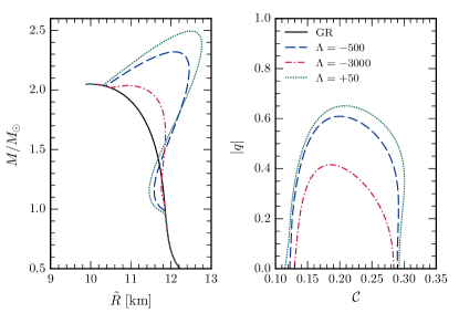
In Fig. 1, we consider what happens when we change the value of while maintaining and fixed. We observe that for sufficiently negative values of the effects of scalarization become suppressed. This can be qualitatively understood from Eq. (90): as we need for scalarization to happen. For fixed values of and , there will be a sufficiently negative value of , for which and scalarization ceases to occur. Although in Fig. 1 we show km2, we have confirmed this by constructing stellar models for even smaller values of . Also, in agreement with Sec. V, we see that alters the threshold for scalarization. This is most clearly seen in the right panel of Fig. 1, where for different values of scalarization starts (evidenced by a nonzero scalar charge ) when different values of compactness are reached.111In the preceding section, because of the weak (scalar) field approximation the Jordan and Einstein frame radii are approximately the same, i.e . This is not the case in this section and hereafter the compactness uses the Jordan frame radius, i.e. . In particular, for , because of the minus sign in the disformal term in Eq. (90), NSs can scalarize for smaller values of , while the opposite happens when . We remark that for large positive the structure equations become singular at the origin as discussed in Sec. IV. This prevents nonrelativistic stars, for which , from scalarizing.
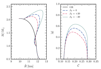
In Fig. 2, we consider what happens when we change the value of while maintaining and fixed. We see that in agreement with Eq. (90), the parameter does not affect the threshold for scalarization. Moreover, we observe that () makes scalarization more (less) evident with respect to . In fact, in Eqs. (48) and (47), we see that and contribute to the scalar field equation through the factors and , which have competing effects in sourcing the scalar field for and . Our numerical integrations indicate that the former is dominant and that affects only very compact NSs ( in the example of Fig. 2).
It is also of interest to see how scalarization affects the interior of NSs. In Fig. 3, we show the normalized pressure profile (top left), the dimensionless mass function (top right), the scalar field (bottom left) and the disformal factor (bottom right) in the stellar interior. The radial coordinate was normalized by the Einstein frame radius . The quantities correspond to three stellar configurations using SLy4 EOS with fixed baryonic mass , which in GR yields a canonical NS with mass , for the sample values of indicated in Table 1. In agreement with our previous discussion we see that NSs with () support a larger (smaller) value of , which translates to a larger (smaller) value of . It is particularly important to observe that is non-negative for all NS models, guaranteeing the Lorentzian signature of spacetime [cf. Eq. (9)].

| [km] | [] | [g cm2] | |||
|---|---|---|---|---|---|
| GR | 11.72 | 1.363 | 1.319 | – | – |
| 11.60 | 1.354 | 1.431 | 0.220 | 0.613 | |
| 11.64 | 1.354 | 1.438 | 0.218 | 0.622 | |
| 11.59 | 1.354 | 1.430 | 0.223 | 0.615 |
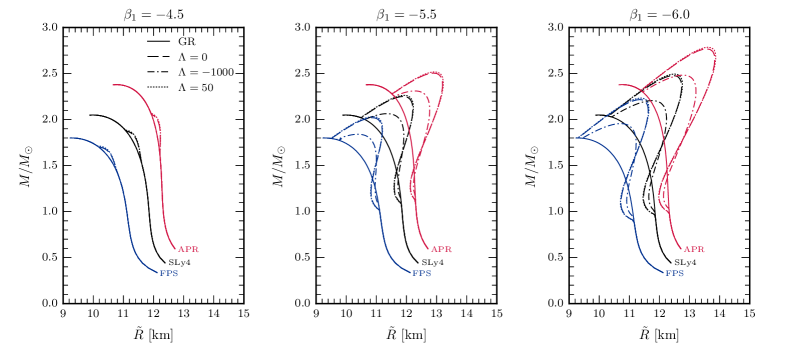
In Fig. 4 we show the mass-radius curves (top panels) and moment of inertia-mass (lower panels) for increasing values of (from left to right), for three realistic EOSs, keeping , but using different values of . As we anticipated in Fig. 1, negative values of reduce the effects of scalarization, while positive values increase them. The case corresponds to the purely conformal theory of Ref. Damour and Esposito-Farèse (1993). We observe that scalarized NS models branch from the GR family at different points for different values of (when is fixed). In agreement with our previous discussion, sufficiently negative values of can completely suppress scalarization. Indeed for the solutions with km2 are identical to GR, while scalarized solutions exist when .
Additionally, we observe degeneracy between families of solutions in theories with different parameters. For instance, the maximum mass for a NS assuming EOS APR is approximately the same, , for both , and , km2. We also point out the degeneracy between the choice of EOS and of the parameters of the theory. For instance, the maximum mass predicted by EOS FPS in the theory with and km2 is approximately the same as that predicted by GR, but for EOS SLy4, i.e . We emphasize that these two types of degeneracies are not exclusive to the theory we are considering, but are generic to any modification to GR Glampedakis et al. (2015).
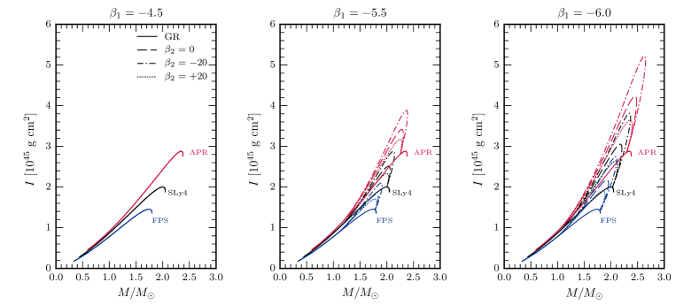
In Fig. 5, we exhibit the mass-radius (top panels) and moment of inertia-mass (lower panels) for increasing values of (from left to right), but now keeping km2 and changing the value of . Once more, sufficiently negative values of can completely suppress scalarization. This is clearly seen in the panels for , where km2, suppresses scalarization for all values of considered. We observe that independently of the choice of EOS, () yields smaller (larger) deviations from GR.


VI.3 Stability of the solutions
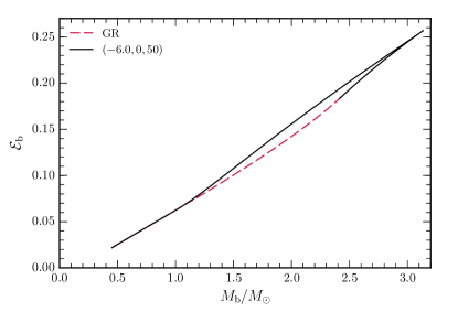
Let us briefly comment on the stability of the scalarized solutions obtained in this section. In general, for a given set of parameters and fixed values of and , we have more than one stellar configuration with different values of the mass . Following the arguments of Refs. Damour and Esposito-Farèse (1993); Harada (1997); Horbatsch and Burgess (2011), we take the solution of smallest mass , i.e., larger fractional binding energy defined in Eq. (63), to be the one which is energetically favorable to be realized in nature. In Fig. 6, we show as a function of for the two families of solutions in a theory with and . The dashed line corresponds to solutions which are indistinguishable from the ones obtained in GR, while the solid line (which branches off from the former around ) corresponds to scalarized solutions. We see that scalarized stellar configurations in our model are energetically favorable, as happens in the case of purely conformal coupling theory Damour and Esposito-Farèse (1993); Harada (1997); Horbatsch and Burgess (2011).
VII An application: EOS-independent - relations
As we have seen in the previous sections the presence of the disformal coupling modifies the structure of NSs making scalar-tensor theories generically predict different bulk properties with respect to GR. However, as we discussed based on Figs. 4 and 5, modifications caused by scalarization are usually degenerate with the choice of EOS, severely limiting our ability to constrain the parameters of the theory using current NS observations (see e.g. Ref. He et al. (2015)). Moreover, different theory parameters can yield similar stellar models for a fixed EOS.
An interesting possibility to circumvent these problems is to search for EOS-independent (or at least weakly EOS-dependent) properties of NSs. Accumulating evidence favoring the existence of such EOS independence between certain properties of NSs, culminated with the discovery of the -Love- relations Yagi and Yunes (2013a, b) connecting the moment of inertia, the tidal Love number and the rotational quadrupole moment (all made dimensionless by certain multiplicative factors) of NSs in GR.
If such relations hold in modified theories of gravitation they can potentially be combined with future NS measurements to constrain competing theories of gravity. This attractive idea was explored in the context of dynamical Chern-Simons theory Yagi and Yunes (2013b), Eddington-inspired Born-Infeld gravity Sham et al. (2014), Einstein-dilaton-Gauss-Bonnet (EdGB) gravity Kleihaus et al. (2014, 2016), theories Doneva et al. (2015) and the Damour-Esposito-Farèse model of scalar-tensor gravity Doneva et al. (2013); Pani and Berti (2014).
Within the present framework we cannot compute the -Love- relations, since while on one hand we can compute , the tidal Love number requires an analysis of tidal interactions, and the rotational quadrupole moment requires pushing the Hartle-Thorne perturbative expansion up to order . Nevertheless, we can investigate whether the recently proposed - relations Breu and Rezzolla (2016) between the moment of inertia and the compactness remain valid in our theory. For a recent study in the Damour-Esposito-Farèse and theories, see Ref. Staykov et al. (2016). This relation was also studied for EdGB and the subclass of Horndeski gravity with nonminimal coupling between the scalar field and the Einstein tensor in Ref. Maselli et al. (2016).
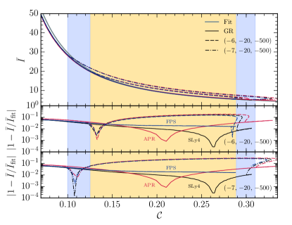
The relation proposed in Ref. Breu and Rezzolla (2016) for the moment of inertia and the compactness is
| (93) |
where the coefficients () are given by , , and . This result is valid for slowly rotating NSs in GR, although it can easily be adapted for rapidly rotating NSs Breu and Rezzolla (2016). The coefficients in Eq. (93) are obtained by fitting the equation to a large sample of EOSs. For earlier work considering a different normalization for , namely , see e.g. Refs. Ravenhall and Pethick (1994); Lattimer and Prakash (2001); Bejger and Haensel (2002); Lattimer and Schutz (2005); Urbanec et al. (2013).
We confront this fit against stellar models in two scalar-tensor theories with the parameters having the values and that support highly scalarized solutions. As seen in Fig. 7, the deviations from GR can be quite large, up to for the theory with in the range of compactness for which spontaneous scalarization happens (cf. Fig. 7, bottom panel). Nevertheless, the EOS independence between and remains even when scalarization occurs (cf. Fig. 7, top panel).
Since our model is largely unconstrained observationally, measurements of the moment of inertia and compactness of NSs could in principle be used to constrain it or, more optimistically, indicate the occurrence of spontaneous scalarization in NSs. This is in contrast with the standard Damour-Esposito-Farèse model, for which the theory’s parameters are so tightly constrained by binary pulsar observations Antoniadis et al. (2012), that spontaneous scalarization (if it exists) is bound to have a negligible influence on the - relation Staykov et al. (2016). We stress however that in general it will be difficult to constrain the parameter space only through the - relation. The reason is in the degeneracy of stellar models for different values of the parameters; see the discussion in Sec. VI.2.
VIII Conclusions and outlook
In this paper we have presented a general formulation to analyze the structure of relativistic stars in scalar-tensor theories with disformal coupling, including the leading-order corrections due to slow rotation. The disformal coupling is negligibly small in comparison with conformal coupling in the weak-gravity or slow-motion regimes, where the scalar field is slowly evolving and typical pressures are much smaller than the energy density scales, but it may be comparable to the ordinary conformal coupling in the strong-gravity regime found inside relativistic stars. Our calculation covers a variety of scalar-tensor models, especially, conformal and disformal couplings to matter, nonstandard scalar kinetic terms and generic scalar potential terms.
After obtaining the stellar structure equations, we have particularly focused on the case of a canonical scalar field with a generic scalar potential. We showed that in the absence of both conformal coupling and a scalar potential, the disformal coupling does not modify the stellar structure with respect to GR. On the other hand, this result shows us that inside relativistic stars the effects of disformal coupling always appear only when there is conformal coupling to matter and/or a nontrivial potential term. The strength of disformal coupling crucially depends on the coupling strength in Eq. (2) with dimensions of (length)2. For a canonical scalar field, has to be of km2 to significantly influence the structure of NSs.
In our numerical analyses, we have investigated the effects of the disformal coupling on the spontaneous scalarization of NSs in the scalar-tensor theory with purely conformal coupling. We found that the effects of disformal coupling depend on the sign of . We showed that for negative values of the mass and moment of inertia of NSs decrease, approaching the values in GR for sufficiently large negative values of . We speculate that this is the consequence of a mechanism similar to the disformal screening proposed in Ref. Koivisto et al. (2012) where in a high density or a large disformal coupling limit the response of the scalar field becomes insensitive to the local matter density, exemplified here by studying relativistic stars. On the other hand, for positive values of , we showed that the mass and moment of inertia increase but for too large positive values of the stellar structure equation becomes singular and a regular NS solution cannot be found. This allowed us to derive a mild upper bound of km2, that does not depend on the choice of the EOS.
We have also tested the applicability of a recently proposed EOS-independent relation between the dimensionless moment of inertia and the compactness for NSs in GR. We found that for a certain domain of the theory’s parameter space, the deviations from GR can be as large as , suggesting that future measurements of NS moment of inertia might be used to test scalar-tensor theories with disformal coupling. Because of the large dimensionality of the parameter space, modifications with respect to GR are generically degenerate between different choices of , and . Thereby, even though deviations from GR can be larger, it seems unlikely that constraints can be put on the theory’s parameters using exclusively the - relation. In this regard, it would be worth extending our work and studying how the -Love- relations are affected by the disformal coupling, generalizing the works of Refs. Pani and Berti (2014); Doneva et al. (2014a, 2013) for scalar-tensor theories with disformal coupling.
Still in this direction, one could investigate whether the “three-hair” relations – EOS-independent relations connecting higher-order multipole moments of rotating NSs in terms of the first three multipole moments in GR Pappas and Apostolatos (2014); Yagi et al. (2014); Majumder et al. (2015) - remain valid in scalar-tensor theory, including those with disformal coupling. This could be accomplished by combining the formalism developed in Pappas and Sotiriou (2015a) with numerical solutions for rotating NSs such as those obtained in Ref. Doneva et al. (2013).
Although the main subject of this paper was to investigate the hydrostatic equilibrium configurations in scalar-tensor theories with disformal coupling, let us briefly comment on the gravitational (core) collapse resulting in the formation of a NS (see e.g. Ref. Gerosa et al. (2016)). A fully numerical analysis of dynamical collapse in this theory is beyond the scope of our paper, but an important issue in this dynamical process may be the possible appearance of ghost instabilities for negative values of Kaloper (2004); Koivisto et al. (2012); Berezhiani et al. (2013); Bettoni and Zumalacarregui (2015). During collapse, matter density at a given position increases, and if at some instant it reaches the threshold value where the effective kinetic term in the scalar field equation vanishes, the time evolution afterwards cannot be determined. For a canonical scalar field , in a linearized approximation where and , the effective kinetic term of the equation of motion (II) is roughly given by
| (94) |
where a dot represents a time derivative. The sign of the kinetic term may change in the region of a critical density higher than . The choice of km2 gives g/cm3, which is a typical central density of NSs. Thus for km2 a NS is not expected to suffer an instability while for other values it might occur in the interior of the star. Of course, for a more precise estimation, nonlinear interactions between the dynamical scalar field, spacetime and matter must be taken into consideration. A detailed study of time-dependent processes in our theory is definitely important, but is left for future work.
Another interesting prospect for future work would be to study compact binaries within our model. The most stringent test of scalar-tensor gravity comes from the measurement of the orbital decay of binaries with asymmetric masses, which constrains the emission of dipolar scalar radiation by the system Freire et al. (2012). We expect that the disformal coupling parameters and should play a role in the orbital evolution of a binary system by influencing the emission of scalar radiation from the system. In fact, both parameters are expected to modify the so-called sensitivities Will and Zaglauer (1989); Zaglauer (1992) that enter at the lowest PN orders sourcing the emission of dipolar scalar radiation. An investigation of compact binaries within our model could, combined with current observational data, yield tight constraints on disformal coupling. Moreover one could study NS solutions for other classes of scalar-tensor theories not considered here. This task is facilitated by the generality of our calculations presented in Sec. III. Work in this direction is currently underway and we hope to report it soon.
Acknowledgements
We would like to thank Andrea Maselli, Emanuele Berti and George Pappas for suggestions on our draft. We thank Jeremy Sakstein and Kent Yagi for several interesting comments and Caio F. B. Macedo for discussions during the development of this work. We also thank the anonymous referee for important suggestions and insightful comments on this work. H.O.S. thanks the hospitality of the Instituto Superior Técnico (Portugal) during the final stages of preparation of this work. This work was supported by FCT-Portugal through Grant No. SFRH/BPD/88299/2012 (M.M.) and a NSF CAREER Grant No. PHY-1055103 (H.O.S.).
Appendix A Disformal invariance
In this appendix, we study how the physical quantities associated with the stellar properties transform under the disformal transformation (2). We write the metrics with slow rotation of spacetimes in the Einstein and Jordan frames as
| (95) |
and
| (96) |
We can relate Eqs. (A) and (A) using the disformal relation (2) as
| (97) | |||||
| (98) | |||||
| (99) | |||||
| (100) |
where we recall that due the symmetries of the problem . From Eqs. (98) and (99) we get
| (101) |
Introducing and in the Einstein and Jordan frames by
| (102) |
and using Eqs. (99) and (101) we find
| (103) |
As it is reasonable to set and at asymptotic infinity, in the class of models considered in the text [Eq. (V)], , and , we find that the ADM mass obtained from the leading-order values of and at asymptotic infinity is disformally invariant
| (104) |
The energy-momentum tensors of the matter fields in the Einstein and Jordan frames are defined by
| (105) |
where () and () are the four-velocity and unit radial vectors in the Einstein (Jordan) frame, respectively Silva et al. (2015). Within the first order of Hartle-Thorne’s slow-rotation approximation Hartle and Thorne (1968), in the Einstein frame
and in the Jordan frame and are defined in the same way as Eq. (A) with an overbar. The nonvanishing components of the energy-momentum tensors in both frames are then given by
| (107a) | |||
| (107b) | |||
and
| (108a) | ||||
| (108b) | ||||
In the Jordan frame, we then make a coordinate transformation from to , such that
| (109) |
Introducing the components of the energy-momentum tensor as (107a)-(107b) with a tilde, we find
| (110) |
and consequently
| (111) |
The components of the energy-momentum tensor in the Einstein and Jordan frames are related by (23) and
| (112) |
Substituting (23), (97), (99), (108a), (108b), (110) and (111) into Eq. (112) we find
| (113) |
Thus from (100),
| (114) |
The angular momenta in the Einstein and Jordan frames are given by
| (115) | |||||
| (116) |
Using again (97), (98), (99), (111) and (112), we find that the angular momentum is disformally invariant
| (117) |
From Eqs. (114) and (117) we find that the moments of inertia in the Einstein and Jordan frames, and , are also disformally invariant
| (118) |
Thus all quantities associated with rotation are disformally invariant. Our arguments in this appendix can be applied to a generic class of the Horndeski theory connected by the disformal transformation Bettoni and Liberati (2013).
References
- Will (2014) C. M. Will, The Confrontation between General Relativity and Experiment, Living Rev. Rel. 17, 4 (2014), arXiv:1403.7377 [gr-qc] .
- Berti et al. (2015) E. Berti et al., Testing General Relativity with Present and Future Astrophysical Observations, Class. Quant. Grav. 32, 243001 (2015), arXiv:1501.07274 [gr-qc] .
- Clifton et al. (2012) T. Clifton, P. G. Ferreira, A. Padilla, and C. Skordis, Modified Gravity and Cosmology, Phys.Rept. 513, 1–189 (2012), arXiv:1106.2476 [astro-ph.CO] .
- Abbott et al. (2016a) B. â. Abbott et al. (Virgo, LIGO Scientific), Observation of Gravitational Waves from a Binary Black Hole Merger, Phys. Rev. Lett. 116, 061102 (2016a), arXiv:1602.03837 [gr-qc] .
- Abbott et al. (2016b) B. P. Abbott et al. (Virgo, LIGO Scientific), Tests of general relativity with GW150914, (2016b), arXiv:1602.03841 [gr-qc] .
- Yunes et al. (2016) N. Yunes, K. Yagi, and F. Pretorius, Theoretical Physics Implications of the Binary Black-Hole Merger GW150914, (2016), arXiv:1603.08955 [gr-qc] .
- Fujii and Maeda (2003) Y. Fujii and K.-I. Maeda, The Scalar-Tensor Theory of Gravitation, by Yasunori Fujii and Kei-ichi Maeda, pp. 256. ISBN 0521811597. Cambridge, UK: Cambridge University Press, March 2003. (Cambridge University Press, 2003).
- Woodard (2015) R. P. Woodard, Ostrogradsky’s theorem on Hamiltonian instability, Scholarpedia 10, 32243 (2015), arXiv:1506.02210 [hep-th] .
- Vainshtein (1972) A. Vainshtein, To the problem of nonvanishing gravitation mass, Phys.Lett. B39, 393–394 (1972).
- Brax et al. (2004) P. Brax, C. van de Bruck, A.-C. Davis, J. Khoury, and A. Weltman, Detecting dark energy in orbit - The Cosmological chameleon, Phys. Rev. D70, 123518 (2004), arXiv:astro-ph/0408415 [astro-ph] .
- Horndeski (1974) G. W. Horndeski, Second-order scalar-tensor field equations in a four-dimensional space, Int.J.Theor.Phys. 10, 363–384 (1974).
- Deffayet et al. (2009a) C. Deffayet, S. Deser, and G. Esposito-Farèse, Generalized Galileons: All scalar models whose curved background extensions maintain second-order field equations and stress-tensors, Phys. Rev. D80, 064015 (2009a), arXiv:0906.1967 [gr-qc] .
- Deffayet et al. (2011) C. Deffayet, X. Gao, D. Steer, and G. Zahariade, From k-essence to generalised Galileons, Phys.Rev. D84, 064039 (2011), arXiv:1103.3260 [hep-th] .
- Kobayashi et al. (2011) T. Kobayashi, M. Yamaguchi, and J. Yokoyama, Generalized G-inflation: Inflation with the most general second-order field equations, Prog. Theor. Phys. 126, 511–529 (2011), arXiv:1105.5723 [hep-th] .
- Damour and Esposito-Farèse (1993) T. Damour and G. Esposito-Farèse, Nonperturbative strong field effects in tensor - scalar theories of gravitation, Phys.Rev.Lett. 70, 2220–2223 (1993).
- Damour and Esposito-Farèse (1996a) T. Damour and G. Esposito-Farèse, Tensor-scalar gravity and binary pulsar experiments, Phys.Rev. D54, 1474–1491 (1996a), arXiv:gr-qc/9602056 [gr-qc] .
- Harada (1997) T. Harada, Stability analysis of spherically symmetric star in scalar-tensor theories of gravity, Prog.Theor.Phys. 98, 359–379 (1997), arXiv:gr-qc/9706014 [gr-qc] .
- Chiba et al. (1997) T. Chiba, T. Harada, and K.-i. Nakao, Gravitational physics in scalar tensor theories: Tests of strong field gravity, Prog.Theor.Phys.Suppl. 128, 335–372 (1997).
- Sotani and Kokkotas (2004) H. Sotani and K. D. Kokkotas, Probing strong-field scalar-tensor gravity with gravitational wave asteroseismology, Phys.Rev. D70, 084026 (2004), arXiv:gr-qc/0409066 [gr-qc] .
- Sotani and Kokkotas (2005) H. Sotani and K. D. Kokkotas, Stellar oscillations in scalar-tensor theory of gravity, Phys.Rev. D71, 124038 (2005), arXiv:gr-qc/0506060 [gr-qc] .
- Sotani (2014) H. Sotani, Scalar gravitational waves from relativistic stars in scalar-tensor gravity, Phys.Rev. D89, 064031 (2014), arXiv:1402.5699 [astro-ph.HE] .
- Silva et al. (2014) H. O. Silva, H. Sotani, E. Berti, and M. Horbatsch, Torsional oscillations of neutron stars in scalar-tensor theory of gravity, Phys. Rev. D90, 124044 (2014), arXiv:1410.2511 [gr-qc] .
- Sotani (2012) H. Sotani, Slowly Rotating Relativistic Stars in Scalar-Tensor Gravity, Phys.Rev. D86, 124036 (2012), arXiv:1211.6986 [astro-ph.HE] .
- Doneva et al. (2013) D. D. Doneva, S. S. Yazadjiev, N. Stergioulas, and K. D. Kokkotas, Rapidly rotating neutron stars in scalar-tensor theories of gravity, Phys.Rev. D88, 084060 (2013), arXiv:1309.0605 [gr-qc] .
- Doneva et al. (2014a) D. D. Doneva, S. S. Yazadjiev, K. V. Staykov, and K. D. Kokkotas, Universal I-Q relations for rapidly rotating neutron and strange stars in scalar-tensor theories, Phys.Rev. D90, 104021 (2014a), arXiv:1408.1641 [gr-qc] .
- Pani and Berti (2014) P. Pani and E. Berti, Slowly rotating neutron stars in scalar-tensor theories, Phys.Rev. D90, 024025 (2014), arXiv:1405.4547 [gr-qc] .
- DeDeo and Psaltis (2004) S. DeDeo and D. Psaltis, Testing strong-field gravity with quasiperiodic oscillations, (2004), arXiv:astro-ph/0405067 [astro-ph] .
- Doneva et al. (2014b) D. D. Doneva, S. S. Yazadjiev, N. Stergioulas, K. D. Kokkotas, and T. M. Athanasiadis, Orbital and epicyclic frequencies around rapidly rotating compact stars in scalar-tensor theories of gravity, Phys.Rev. D90, 044004 (2014b), arXiv:1405.6976 [astro-ph.HE] .
- Pappas and Sotiriou (2015a) G. Pappas and T. P. Sotiriou, Multipole moments in scalar-tensor theory of gravity, Phys. Rev. D91, 044011 (2015a), arXiv:1412.3494 [gr-qc] .
- Pappas and Sotiriou (2015b) G. Pappas and T. P. Sotiriou, Geodesic properties in terms of multipole moments in scalar–-tensor theories of gravity, Mon. Not. Roy. Astron. Soc. 453, 2862–2876 (2015b), arXiv:1505.02882 [gr-qc] .
- Novak (1998a) J. Novak, Neutron star transition to strong scalar field state in tensor scalar gravity, Phys.Rev. D58, 064019 (1998a), arXiv:gr-qc/9806022 [gr-qc] .
- Harada et al. (1997) T. Harada, T. Chiba, K.-i. Nakao, and T. Nakamura, Scalar gravitational wave from Oppenheimer-Snyder collapse in scalar - tensor theories of gravity, Phys.Rev. D55, 2024–2037 (1997), arXiv:gr-qc/9611031 [gr-qc] .
- Novak (1998b) J. Novak, Spherical neutron star collapse in tensor - scalar theory of gravity, Phys.Rev. D57, 4789–4801 (1998b), arXiv:gr-qc/9707041 [gr-qc] .
- Gerosa et al. (2016) D. Gerosa, U. Sperhake, and C. D. Ott, Numerical simulations of stellar collapse in scalar-tensor theories of gravity, (2016), arXiv:1602.06952 [gr-qc] .
- Horbatsch and Burgess (2011) M. Horbatsch and C. Burgess, Semi-Analytic Stellar Structure in Scalar-Tensor Gravity, JCAP 1108, 027 (2011), arXiv:1006.4411 [gr-qc] .
- Lima et al. (2010) W. C. Lima, G. E. Matsas, and D. A. Vanzella, Awaking the vacuum in relativistic stars, Phys.Rev.Lett. 105, 151102 (2010), arXiv:1009.1771 [gr-qc] .
- Landulfo et al. (2012) A. G. S. Landulfo, W. C. C. Lima, G. E. A. Matsas, and D. A. T. Vanzella, Particle creation due to tachyonic instability in relativistic stars, Phys. Rev. D86, 104025 (2012), arXiv:1204.3654 [gr-qc] .
- Mendes et al. (2014a) R. F. Mendes, G. E. Matsas, and D. A. Vanzella, Quantum versus classical instability of scalar fields in curved backgrounds, Phys.Rev. D89, 047503 (2014a), arXiv:1310.2185 [gr-qc] .
- Landulfo et al. (2015) A. G. S. Landulfo, W. C. C. Lima, G. E. A. Matsas, and D. A. T. Vanzella, From quantum to classical instability in relativistic stars, Phys.Rev. D91, 024011 (2015), arXiv:1410.2274 [gr-qc] .
- Mendes et al. (2014b) R. F. P. Mendes, G. E. A. Matsas, and D. A. T. Vanzella, Instability of nonminimally coupled scalar fields in the spacetime of slowly rotating compact objects, Phys. Rev. D90, 044053 (2014b), arXiv:1407.6405 [gr-qc] .
- Pani et al. (2011) P. Pani, V. Cardoso, E. Berti, J. Read, and M. Salgado, The vacuum revealed: the final state of vacuum instabilities in compact stars, Phys.Rev. D83, 081501 (2011), arXiv:1012.1343 [gr-qc] .
- Yagi et al. (2012) K. Yagi, L. C. Stein, N. Yunes, and T. Tanaka, Post-Newtonian, Quasi-Circular Binary Inspirals in Quadratic Modified Gravity, Phys.Rev. D85, 064022 (2012), arXiv:1110.5950 [gr-qc] .
- Yagi et al. (2016) K. Yagi, L. C. Stein, and N. Yunes, Challenging the Presence of Scalar Charge and Dipolar Radiation in Binary Pulsars, Phys. Rev. D93, 024010 (2016), arXiv:1510.02152 [gr-qc] .
- Barausse and Yagi (2015) E. Barausse and K. Yagi, Gravitation-Wave Emission in Shift-Symmetric Horndeski Theories, Phys. Rev. Lett. 115, 211105 (2015), arXiv:1509.04539 [gr-qc] .
- Psaltis (2008) D. Psaltis, Probes and Tests of Strong-Field Gravity with Observations in the Electromagnetic Spectrum, Living Rev. Rel. 11, 9 (2008), arXiv:0806.1531 [astro-ph] .
- Yunes and Siemens (2013) N. Yunes and X. Siemens, Gravitational-Wave Tests of General Relativity with Ground-Based Detectors and Pulsar Timing-Arrays, Living Rev.Rel. 16, 9 (2013), arXiv:1304.3473 [gr-qc] .
- Barausse et al. (2013) E. Barausse, C. Palenzuela, M. Ponce, and L. Lehner, Neutron-star mergers in scalar-tensor theories of gravity, Phys.Rev. D87, 081506 (2013), arXiv:1212.5053 [gr-qc] .
- Palenzuela et al. (2014) C. Palenzuela, E. Barausse, M. Ponce, and L. Lehner, Dynamical scalarization of neutron stars in scalar-tensor gravity theories, Phys.Rev. D89, 044024 (2014), arXiv:1310.4481 [gr-qc] .
- Taniguchi et al. (2015) K. Taniguchi, M. Shibata, and A. Buonanno, Quasiequilibrium sequences of binary neutron stars undergoing dynamical scalarization, Phys. Rev. D91, 024033 (2015), arXiv:1410.0738 [gr-qc] .
- Sennett and Buonanno (2016) N. Sennett and A. Buonanno, Modeling dynamical scalarization with a resummed post-Newtonian expansion, (2016), arXiv:1603.03300 [gr-qc] .
- Cardoso et al. (2013a) V. Cardoso, I. P. Carucci, P. Pani, and T. P. Sotiriou, Black holes with surrounding matter in scalar-tensor theories, Phys.Rev.Lett. 111, 111101 (2013a), arXiv:1308.6587 [gr-qc] .
- Cardoso et al. (2013b) V. Cardoso, I. P. Carucci, P. Pani, and T. P. Sotiriou, Matter around Kerr black holes in scalar-tensor theories: scalarization and superradiant instability, Phys.Rev. D88, 044056 (2013b), arXiv:1305.6936 [gr-qc] .
- Freire et al. (2012) P. C. Freire, N. Wex, G. Esposito-Farèse, J. P. Verbiest, M. Bailes, et al., The relativistic pulsar-white dwarf binary PSR J1738+0333 II. The most stringent test of scalar-tensor gravity, Mon. Not. Roy. Astron. Soc. 423, 3328 (2012), arXiv:1205.1450 [astro-ph.GA] .
- Harada (1998) T. Harada, Neutron stars in scalar tensor theories of gravity and catastrophe theory, Phys.Rev. D57, 4802–4811 (1998), arXiv:gr-qc/9801049 [gr-qc] .
- Silva et al. (2015) H. O. Silva, C. F. B. Macedo, E. Berti, and L. C. B. Crispino, Slowly rotating anisotropic neutron stars in general relativity and scalar–tensor theory, Class. Quant. Grav. 32, 145008 (2015), arXiv:1411.6286 [gr-qc] .
- Mendes (2015) R. F. P. Mendes, Possibility of setting a new constraint to scalar-tensor theories, Phys. Rev. D91, 064024 (2015), arXiv:1412.6789 [gr-qc] .
- Palenzuela and Liebling (2016) C. Palenzuela and S. L. Liebling, Constraining scalar-tensor theories of gravity from the most massive neutron stars, Phys. Rev. D93, 044009 (2016), arXiv:1510.03471 [gr-qc] .
- Mendes and Ortiz (2016) R. F. P. Mendes and N. Ortiz, Highly compact neutron stars in scalar-tensor theories of gravity: spontaneous scalarization vs. gravitational collapse, (2016), arXiv:1604.04175 [gr-qc] .
- Deffayet et al. (2009b) C. Deffayet, G. Esposito-Farèse, and A. Vikman, Covariant Galileon, Phys.Rev. D79, 084003 (2009b), arXiv:0901.1314 [hep-th] .
- Bettoni and Liberati (2013) D. Bettoni and S. Liberati, Disformal invariance of second order scalar-tensor theories: Framing the Horndeski action, Phys. Rev. D88, 084020 (2013), arXiv:1306.6724 [gr-qc] .
- Zumalacárregui and García-Bellido (2014) M. Zumalacárregui and J. García-Bellido, Transforming gravity: from derivative couplings to matter to second-order scalar-tensor theories beyond the Horndeski Lagrangian, Phys. Rev. D89, 064046 (2014), arXiv:1308.4685 [gr-qc] .
- Bekenstein (1993) J. D. Bekenstein, The Relation between physical and gravitational geometry, Phys. Rev. D48, 3641–3647 (1993), arXiv:gr-qc/9211017 [gr-qc] .
- Koivisto (2008) T. S. Koivisto, Disformal quintessence, (2008), arXiv:0811.1957 [astro-ph] .
- Sakstein (2015) J. Sakstein, Towards Viable Cosmological Models of Disformal Theories of Gravity, Phys. Rev. D91, 024036 (2015), arXiv:1409.7296 [astro-ph.CO] .
- Sakstein and Verner (2015) J. Sakstein and S. Verner, Disformal Gravity Theories: A Jordan Frame Analysis, Phys. Rev. D92, 123005 (2015), arXiv:1509.05679 [gr-qc] .
- Zumalacarregui et al. (2013) M. Zumalacarregui, T. S. Koivisto, and D. F. Mota, DBI Galileons in the Einstein Frame: Local Gravity and Cosmology, Phys. Rev. D87, 083010 (2013), arXiv:1210.8016 [astro-ph.CO] .
- Koivisto et al. (2014) T. Koivisto, D. Wills, and I. Zavala, Dark D-brane Cosmology, JCAP 1406, 036 (2014), arXiv:1312.2597 [hep-th] .
- Bekenstein (2004) J. D. Bekenstein, Relativistic gravitation theory for the MOND paradigm, Phys.Rev. D70, 083509 (2004), arXiv:astro-ph/0403694 [astro-ph] .
- Bekenstein and Sanders (1994) J. D. Bekenstein and R. H. Sanders, Gravitational lenses and unconventional gravity theories, Astrophys. J. 429, 480 (1994), arXiv:astro-ph/9311062 [astro-ph] .
- de Rham et al. (2011) C. de Rham, G. Gabadadze, and A. J. Tolley, Resummation of Massive Gravity, Phys.Rev.Lett. 106, 231101 (2011), arXiv:1011.1232 [hep-th] .
- de Rham and Gabadadze (2010) C. de Rham and G. Gabadadze, Generalization of the Fierz-Pauli Action, Phys.Rev. D82, 044020 (2010), arXiv:1007.0443 [hep-th] .
- Berezhiani et al. (2013) L. Berezhiani, G. Chkareuli, and G. Gabadadze, Restricted Galileons, Phys. Rev. D88, 124020 (2013), arXiv:1302.0549 [hep-th] .
- Brito et al. (2014) R. Brito, A. Terrana, M. Johnson, and V. Cardoso, Nonlinear dynamical stability of infrared modifications of gravity, Phys.Rev. D90, 124035 (2014), arXiv:1409.0886 [hep-th] .
- Magueijo (2003) J. Magueijo, New varying speed of light theories, Rept. Prog. Phys. 66, 2025 (2003), arXiv:astro-ph/0305457 [astro-ph] .
- Kaloper (2004) N. Kaloper, Disformal inflation, Phys. Lett. B583, 1–13 (2004), arXiv:hep-ph/0312002 [hep-ph] .
- van de Bruck et al. (2016) C. van de Bruck, T. Koivisto, and C. Longden, Disformally coupled inflation, JCAP 1603, 006 (2016), arXiv:1510.01650 [astro-ph.CO] .
- Creminelli et al. (2014) P. Creminelli, J. Gleyzes, J. Norena, and F. Vernizzi, Resilience of the standard predictions for primordial tensor modes, Phys. Rev. Lett. 113, 231301 (2014), arXiv:1407.8439 [astro-ph.CO] .
- Minamitsuji (2014) M. Minamitsuji, Disformal transformation of cosmological perturbations, Phys. Lett. B737, 139–150 (2014), arXiv:1409.1566 [astro-ph.CO] .
- Tsujikawa (2015) S. Tsujikawa, Disformal invariance of cosmological perturbations in a generalized class of Horndeski theories, JCAP 1504, 043 (2015), arXiv:1412.6210 [hep-th] .
- Watanabe et al. (2015) Y. Watanabe, A. Naruko, and M. Sasaki, Multi-disformal invariance of non-linear primordial perturbations, Europhys. Lett. 111, 39002 (2015), arXiv:1504.00672 [gr-qc] .
- Motohashi and White (2016) H. Motohashi and J. White, Disformal invariance of curvature perturbation, JCAP 1602, 065 (2016), arXiv:1504.00846 [gr-qc] .
- Domenech et al. (2015) G. Domenech, A. Naruko, and M. Sasaki, Cosmological disformal invariance, JCAP 1510, 067 (2015), arXiv:1505.00174 [gr-qc] .
- Sakstein (2014) J. Sakstein, Disformal Theories of Gravity: From the Solar System to Cosmology, JCAP 1412, 012 (2014), arXiv:1409.1734 [astro-ph.CO] .
- van de Bruck and Morrice (2015) C. van de Bruck and J. Morrice, Disformal couplings and the dark sector of the universe, JCAP 1504, 036 (2015), arXiv:1501.03073 [gr-qc] .
- Zumalacarregui et al. (2010) M. Zumalacarregui, T. S. Koivisto, D. F. Mota, and P. Ruiz-Lapuente, Disformal Scalar Fields and the Dark Sector of the Universe, JCAP 1005, 038 (2010), arXiv:1004.2684 [astro-ph.CO] .
- Koivisto et al. (2012) T. S. Koivisto, D. F. Mota, and M. Zumalacarregui, Screening Modifications of Gravity through Disformally Coupled Fields, Phys. Rev. Lett. 109, 241102 (2012), arXiv:1205.3167 [astro-ph.CO] .
- De Felice and Tsujikawa (2012) A. De Felice and S. Tsujikawa, Conditions for the cosmological viability of the most general scalar-tensor theories and their applications to extended Galileon dark energy models, JCAP 1202, 007 (2012), arXiv:1110.3878 [gr-qc] .
- Bettoni et al. (2012) D. Bettoni, V. Pettorino, S. Liberati, and C. Baccigalupi, Non-minimally coupled dark matter: effective pressure and structure formation, JCAP 1207, 027 (2012), arXiv:1203.5735 [astro-ph.CO] .
- Hagala et al. (2016) R. Hagala, C. Llinares, and D. F. Mota, Cosmological simulations with disformally coupled symmetron fields, Astron. Astrophys. 585, A37 (2016), arXiv:1504.07142 [astro-ph.CO] .
- Ip et al. (2015) H. Y. Ip, J. Sakstein, and F. Schmidt, Solar System Constraints on Disformal Gravity Theories, JCAP 1510, 051 (2015), arXiv:1507.00568 [gr-qc] .
- Noller (2012) J. Noller, Derivative Chameleons, JCAP 1207, 013 (2012), arXiv:1203.6639 [gr-qc] .
- Brax and Burrage (2014) P. Brax and C. Burrage, Constraining Disformally Coupled Scalar Fields, Phys. Rev. D90, 104009 (2014), arXiv:1407.1861 [astro-ph.CO] .
- Brax and Burrage (2015) P. Brax and C. Burrage, Explaining the Proton Radius Puzzle with Disformal Scalars, Phys. Rev. D91, 043515 (2015), arXiv:1407.2376 [hep-ph] .
- Brax et al. (2015a) P. Brax, C. Burrage, A.-C. Davis, and G. Gubitosi, Cosmological Tests of Coupled Galileons, JCAP 1503, 028 (2015a), arXiv:1411.7621 [astro-ph.CO] .
- Lamm (2015) H. Lamm, Can Galileons solve the muon problem? Phys. Rev. D92, 055007 (2015), arXiv:1505.00057 [hep-ph] .
- Brax et al. (2015b) P. Brax, C. Burrage, and C. Englert, Disformal dark energy at colliders, Phys. Rev. D92, 044036 (2015b), arXiv:1506.04057 [hep-ph] .
- van de Bruck et al. (2013) C. van de Bruck, J. Morrice, and S. Vu, Constraints on Nonconformal Couplings from the Properties of the Cosmic Microwave Background Radiation, Phys. Rev. Lett. 111, 161302 (2013), arXiv:1303.1773 [astro-ph.CO] .
- Brax et al. (2013) P. Brax, C. Burrage, A.-C. Davis, and G. Gubitosi, Cosmological Tests of the Disformal Coupling to Radiation, JCAP 1311, 001 (2013), arXiv:1306.4168 [astro-ph.CO] .
- van de Bruck et al. (2015) C. van de Bruck, J. Mifsud, and N. J. Nunes, The variation of the fine-structure constant from disformal couplings, JCAP 1512, 018 (2015), arXiv:1510.00200 [astro-ph.CO] .
- Neveu et al. (2014) J. Neveu, V. Ruhlmann-Kleider, P. Astier, M. Besancon, A. Conley, J. Guy, A. Moller, N. Palanque-Delabrouille, and E. Babichev, First experimental constraints on the disformally coupled Galileon model, Astron. Astrophys. 569, A90 (2014), arXiv:1403.0854 [gr-qc] .
- Iorio (2014) L. Iorio, Constraining on the Preferred-Frame , parameters from Solar System planetary precessions, Int. J. Mod. Phys. D23, 1450006 (2014), arXiv:1210.3026 [gr-qc] .
- Bertotti et al. (2003) B. Bertotti, L. Iess, and P. Tortora, A test of general relativity using radio links with the Cassini spacecraft, Nature 425, 374 (2003).
- Koivisto and Nyrhinen (2015) T. Koivisto and H. J. Nyrhinen, Stability of disformally coupled accretion disks, (2015), arXiv:1503.02063 [gr-qc] .
- Bowers and Liang (1974) R. L. Bowers and E. P. T. Liang, Anisotropic Spheres in General Relativity, Astrophys. J. 188, 657 (1974).
- Hartle (1967) J. B. Hartle, Slowly rotating relativistic stars. I. Equations of structure, Astrophys.J. 150, 1005–1029 (1967).
- Hartle and Thorne (1968) J. B. Hartle and K. S. Thorne, Slowly Rotating Relativistic Stars. II. Models for Neutron Stars and Supermassive Stars, Astrophys.J. 153, 807 (1968).
- Ramazanoğlu and Pretorius (2016) F. M. Ramazanoğlu and F. Pretorius, Spontaneous Scalarization with Massive Fields, (2016), arXiv:1601.07475 [gr-qc] .
- Yazadjiev et al. (2016) S. S. Yazadjiev, D. D. Doneva, and D. Popchev, Slowly rotating neutron stars in scalar-tensor theories with a massive scalar field, (2016), arXiv:1602.04766 [gr-qc] .
- Chen et al. (2015) P. Chen, T. Suyama, and J. Yokoyama, Spontaneous scalarization: asymmetron as dark matter, Phys. Rev. D92, 124016 (2015), arXiv:1508.01384 [gr-qc] .
- Bettoni and Zumalacarregui (2015) D. Bettoni and M. Zumalacarregui, Kinetic mixing in scalar-tensor theories of gravity, Phys. Rev. D91, 104009 (2015), arXiv:1502.02666 [gr-qc] .
- Damour and Esposito-Farèse (1996b) T. Damour and G. Esposito-Farèse, Testing gravity to second post-Newtonian order: A Field theory approach, Phys.Rev. D53, 5541–5578 (1996b), arXiv:gr-qc/9506063 [gr-qc] .
- Harrison et al. (1965) B. K. Harrison, K. S. Thorne, M. Wakano, and J. A. Wheeler, Gravitation Theory and Gravitational Collapse, Chicago: University of Chicago Press, 1965 (1965).
- Akmal et al. (1998) A. Akmal, V. Pandharipande, and D. Ravenhall, The Equation of state of nucleon matter and neutron star structure, Phys.Rev. C58, 1804–1828 (1998), arXiv:nucl-th/9804027 [nucl-th] .
- Douchin and Haensel (2001) F. Douchin and P. Haensel, A unified equation of state of dense matter and neutron star structure, Astron. Astrophys. 380, 151 (2001), arXiv:astro-ph/0111092 [astro-ph] .
- Friedman and Pandharipande (1981) B. Friedman and V. Pandharipande, Hot and cold, nuclear and neutron matter, Nucl.Phys. A361, 502–520 (1981).
- Demorest et al. (2010) P. Demorest, T. Pennucci, S. Ransom, M. Roberts, and J. Hessels, Shapiro Delay Measurement of A Two Solar Mass Neutron Star, Nature 467, 1081–1083 (2010), arXiv:1010.5788 [astro-ph.HE] .
- Glampedakis et al. (2015) K. Glampedakis, G. Pappas, H. O. Silva, and E. Berti, Post-Tolman-Oppenheimer-Volkoff formalism for relativistic stars, Phys. Rev. D92, 024056 (2015), arXiv:1504.02455 [gr-qc] .
- He et al. (2015) X.-T. He, F. J. Fattoyev, B.-A. Li, and W. G. Newton, Impact of the equation-of-state–gravity degeneracy on constraining the nuclear symmetry energy from astrophysical observables, Phys. Rev. C91, 015810 (2015), arXiv:1408.0857 [nucl-th] .
- Yagi and Yunes (2013a) K. Yagi and N. Yunes, I-Love-Q, Science 341, 365–368 (2013a), arXiv:1302.4499 [gr-qc] .
- Yagi and Yunes (2013b) K. Yagi and N. Yunes, I-Love-Q Relations in Neutron Stars and their Applications to Astrophysics, Gravitational Waves and Fundamental Physics, Phys.Rev. D88, 023009 (2013b), arXiv:1303.1528 [gr-qc] .
- Sham et al. (2014) Y. H. Sham, L. M. Lin, and P. Leung, Testing universal relations of neutron stars with a nonlinear matter-gravity coupling theory, Astrophys.J. 781, 66 (2014), arXiv:1312.1011 [gr-qc] .
- Kleihaus et al. (2014) B. Kleihaus, J. Kunz, and S. Mojica, Quadrupole Moments of Rapidly Rotating Compact Objects in Dilatonic Einstein-Gauss-Bonnet Theory, Phys. Rev. D90, 061501 (2014), arXiv:1407.6884 [gr-qc] .
- Kleihaus et al. (2016) B. Kleihaus, J. Kunz, S. Mojica, and M. Zagermann, Rapidly Rotating Neutron Stars in Dilatonic Einstein-Gauss-Bonnet Theory, (2016), arXiv:1601.05583 [gr-qc] .
- Doneva et al. (2015) D. D. Doneva, S. S. Yazadjiev, and K. D. Kokkotas, The I-Q relations for rapidly rotating neutron stars in gravity, Phys. Rev. D92, 064015 (2015), arXiv:1507.00378 [gr-qc] .
- Breu and Rezzolla (2016) C. Breu and L. Rezzolla, Maximum mass, moment of inertia and compactness of relativistic stars, (2016), arXiv:1601.06083 [gr-qc] .
- Staykov et al. (2016) K. V. Staykov, D. D. Doneva, and S. S. Yazadjiev, Moment of inertia-compactness universal relations in scalar-tensor theories and gravity, (2016), arXiv:1602.00504 [gr-qc] .
- Maselli et al. (2016) A. Maselli, H. O. Silva, M. Minamitsuji, and E. Berti, Fab Four Neutron Stars, (2016), arXiv:1603.04876 [gr-qc] .
- Ravenhall and Pethick (1994) D. G. Ravenhall and C. J. Pethick, Neutron star moments of inertia, Astrophys. J. 424, 846–851 (1994).
- Lattimer and Prakash (2001) J. Lattimer and M. Prakash, Neutron star structure and the equation of state, Astrophys.J. 550, 426 (2001), arXiv:astro-ph/0002232 [astro-ph] .
- Bejger and Haensel (2002) M. Bejger and P. Haensel, Moments of inertia for neutron and strange stars: Limits derived for the Crab pulsar, Astron.Astrophys. 396, 917 (2002), arXiv:astro-ph/0209151 [astro-ph] .
- Lattimer and Schutz (2005) J. M. Lattimer and B. F. Schutz, Constraining the equation of state with moment of inertia measurements, Astrophys.J. 629, 979–984 (2005), arXiv:astro-ph/0411470 [astro-ph] .
- Urbanec et al. (2013) M. Urbanec, J. C. Miller, and Z. Stuchlik, Quadrupole moments of rotating neutron stars and strange stars, Mon. Not. Roy. Astron. Soc. 433, 1903 (2013), arXiv:1301.5925 [astro-ph.SR] .
- Antoniadis et al. (2012) J. Antoniadis, M. van Kerkwijk, D. Koester, P. Freire, N. Wex, et al., The relativistic pulsar-white dwarf binary PSR J1738+0333 I. Mass determination and evolutionary history, Mon.Not.Roy.Astron.Soc. 423, 3316 (2012), arXiv:1204.3948 [astro-ph.HE] .
- Pappas and Apostolatos (2014) G. Pappas and T. A. Apostolatos, Effectively universal behavior of rotating neutron stars in general relativity makes them even simpler than their Newtonian counterparts, Phys.Rev.Lett. 112, 121101 (2014), arXiv:1311.5508 [gr-qc] .
- Yagi et al. (2014) K. Yagi, K. Kyutoku, G. Pappas, N. Yunes, and T. A. Apostolatos, Effective No-Hair Relations for Neutron Stars and Quark Stars: Relativistic Results, Phys.Rev. D89, 124013 (2014), arXiv:1403.6243 [gr-qc] .
- Majumder et al. (2015) B. Majumder, K. Yagi, and N. Yunes, Improved Universality in the Neutron Star Three-Hair Relations, Phys. Rev. D92, 024020 (2015), arXiv:1504.02506 [gr-qc] .
- Will and Zaglauer (1989) C. M. Will and H. W. Zaglauer, Gravitational Radiation, Close Binary Systems, and the Brans-dicke Theory of Gravity, Astrophys. J. 346, 366 (1989).
- Zaglauer (1992) H. Zaglauer, Neutron stars and gravitational scalars, Astrophys.J. 393, 685–696 (1992).