Invisible Axion-Like Dark Matter from Electroweak Bosonic Seesaw

Abstract

We explore a model based on the classically-scale invariant standard model (SM) with a strongly coupled vector-like dynamics, which is called hypercolor (HC). The scale symmetry is dynamically broken by the vector-like condensation at the TeV scale, so that the SM Higgs acquires the negative mass-squared by the bosonic seesaw mechanism to realize the electroweak symmetry breaking. An elementary pseudoscalar $S$ is introduced to give masses for the composite Nambu-Goldstone bosons (HC pions): the HC pion can be a good target to explore through a diphoton channel at the LHC. As the consequence of the bosonic seesaw, the fluctuating mode of $S$, which we call $s$, develops tiny couplings to the SM particles and is predicted to be very light. The $s$ predominantly decays to diphoton and can behave as an invisible axion-like dark matter. The mass of the $s$-dark matter is constrained by currently available cosmological and astrophysical limits to be $10^{-4}{\rm eV}\lesssim m_{s}\lesssim 1\,{\rm eV}$. We find that the sufficient amount of relic abundance for the $s$-dark matter can be accumulated via the coherent oscillation. The detection potential in microwave cavity experiments is also addressed.

I Introduction

Discovery of the Higgs boson Aad:2012tfa ; Chatrchyan:2013lba has made up for the last piece of the standard model (SM) in terms of the particle content, though the Higgs physics such as the coupling property is still uncertain. The Higgs boson in the SM plays the important role for the electroweak symmetry breaking, which is triggered by the nonzero vacuum expectation value of the Higgs field with the negative mass-squared. The Higgs mass term can be necessarily introduced once the Higgs field is put in, due to the renormalizability upon which the SM has been established. However, the Higgs mass term still involves unsatisfactory ingredients on the theoretical ground: one is called the gauge hierarchy problem, that is what we need to answer: how to stabilize the electroweak vacuum. The other, which would be correlated with the former, is the origin of the “negative”-mass squared, which is simply assumed in the SM without any dynamical concept.

One intriguing idea to solve those problems is to assume the classical-scale invariance in the SM. In this approach, there is no dimensionful parameter at a classical level, so one does not need to take care of quadratic divergent terms regarding the renormalization of the Higgs boson mass: thus no scale is present in the model, which would be anomalously generated, e.g., via the radiative breaking. The classical-scale symmetry is then broken by the Coleman-Weinberg mechanism Coleman:1973jx , which generates the mass scale via dimensional transmutation.

Actually, such a radiative-breaking scenario does not work solely within the SM itself, due to the presence of the heavy top quark, so one is eventually forced to add extra degrees of freedom to trigger the radiative breaking as desired. One of the way out along this approach would be to extend the SM gauge symmetry by introducing an extra $U(1)$ gauge symmetry Hempfling:1996ht . However, most of such models suffer from an ad hoc assumption: one requires to assume the sign of the quartic coupling between the SM Higgs boson and an additional scalar field to be negative.

This “sign problem” can be solved in a way of a dynamical mechanism, which is called bosonic seesaw mechanism BSS . The mechanism itself is essentially analogue to the usual type-I seesaw mechanism, well-known in addressing the neutrino sector. The key point to note is that in the case of fermions, the phase of mass term can be absorbed by redefinition of the fermion fields, just by the $U(1)_{A}$ phase rotation. In contrast, the phase cannot be removed by any ways for boson mass terms, rather will be physical once the negative sign shows up in the bosonic sector. Thus models having the bosonic seesaw mechanism built based on the classical-scale invariance can realize the desired situation in which the problems raised above can be settled down by a dynamical explanation.

Recently, such a hybrid model encoding both the classical-scale invariance and bosonic seesaw mechanism has been proposed Haba:2015qbz . The model in Ref. Haba:2015qbz is constructed based on the classically-scale invariant SM plus a vector-like strongly coupled sector, which we call hypercolor (HC) (which was originally quoted as “technicolor” in Ref. Haba:2015qbz ). In the model the classical-scale invariance is dynamically broken by the vector-like condensation of the HC fermion bilinear, triggered by the strongly coupled HC, in a way analogous to QCD. The negative mass-squared of the Higgs is induced by the bosonic seesaw mechanism through the mixing between the elementary Higgs doublet and the composite-HC Higgs doublet formed as the HC fermion bound state. Thus, the HC dynamics plays the essential role to solve both the gauge hierarchy and negative-mass squared problems.

In the model of Haba:2015qbz the success of the bosonic seesaw by the HC dynamics is subject to the presence of the “chiral” symmetry carried by the HC fermions, which is partially vector-like gauged by the electroweak charges to provide the composite-HC Higgs doublet with the appropriate SM charges. When the HC fermion condensate develops to be nonzero, the “chiral” symmetry is dynamically broken down to the vectorial subgroup, at the same time the scale symmetry is broken. This leads to a couple of Nambu-Goldstone bosons (HC pions).

The origin of mass for the HC pions in the model of Haba:2015qbz is responsible for a pseudoscalar $S$, having the Yukawa coupling to the HC fermions explicitly breaking the “chiral” symmetry: the pseudoscalar $S$ develops the nonzero vacuum expectation value as the direct consequence of the bosonic seesaw, to give the HC pion masses via the Yukawa coupling, hence acts as another “Higgs” for the HC pions. Thus, discovering the pseudoscalar $S$ as well as the HC pions is a direct probe and a smoking-gun for this bosonic seesaw model.

In this paper, we discuss the phenomenological consequence of the pseudoscalar $S$ linking to the presence of the HC pions, crucial for the bosonic seesaw model of Ref. Haba:2015qbz . We find that, after the dynamical-scale breaking and triggering the electroweak bosonic seesaw at a TeV scale, the fluctuating mode of $S$, which is denoted as $s$, develops vanishingly small couplings to the SM particles. It turns out, furthermore, that in close relation to the HC pion masses the $s$ mass is predicted to be very light and to predominantly decay to diphoton. We then identify the $s$ as a dark matter candidate like an invisible axion-like particle and constrain the $s$ mass by several cosmological and astrophysical bounds. The $s$ mass is thus limited to be $10^{-4}\,{\rm eV}\lesssim m_{s}\lesssim 1\,{\rm eV}$.

We examine the possibility of the cosmological productions of the $s$ and show that the $s$ is unlikely to be thermally produced essentially due to its tiny couplings to the HC sector in the thermal equilibrium. We then find that the sufficient amount of relic abundance of $s$ as the cold dark matter can be accumulated via the coherent oscillation, just like the invisible axion case. The detection potential in microwave cavity experiments is also addressed. It is shown that the $s$ with mass around $1\,{\rm eV}$ can have the same level of the detection sensibility as that of the axion in the currently equipped experimental setup, so the $s$ is detectable by the microwave cavity experiments.

This paper is organized as follows: in Sec. II we first review the model of Ref. Haba:2015qbz by focusing on the essential points to realize the electroweak symmetry breaking via the bosonic seesaw and to give masses to the HC pions. (The details for the calculation of the HC pions signals are given in a couple of Appendices.) In Sec. III we show the close relationship between masses of the pseudoscalar $s$ and the HC pions, and the $s$ couplings to the SM particles arising as the direct consequence of the bosonic seesaw mechanism, which turns out to be vanishingly small. We then identify the $s$ as a dark matter candidate and constrain the mass by several cosmological and astrophysical bounds currently at hand. In Sec. IV we discuss the cosmological productions of the $s$ involving the thermal and non-thermal processes. It is shown that the relic abundance of the $s$ cannot be thermally produced enough to account for the present dark matter density due to the tiny couplings to the SM particles. We then find that the non-thermal production, namely, the coherent oscillation is dominant in the production mechanism for the $s$, which is sufficient for the $s$ to be a cold dark matter in the present universe. The detection potential of the $s$-dark mater in microwave cavity experiments are also discussed in comparison with the case of invisible axion-like particles. Summary and discussion are given in Sec. V.

Appendix A provides the details for computation of the HC pion masses, and Appendix B gives derivation of the HC pion couplings based on the nonlinear realization of the “chiral” symmetry. The $s$ couplings are also generated there due to the mixing with the HC eta-prime arising through the bosonic seesaw. In Appendix C we present the decay properties of the HC pions relevant to the LHC study, and show the details of the LHC production cross sections to compute the 750 GeV HC pion signals, in comparison with the current LHC bounds.

II A hypercolor model with bosonic seesaw mechanism

The model we employ is based on the classically-scale invariant SM plus a strongly coupled HC dynamics at the TeV scale. The way to construct the model follows from the literature Haba:2015qbz . The HC sector is described by the HC-gluon ${\cal G}$ with a gauge coupling $g_{\rm HC}$ and three vector-like fermion triplets , $F_{L,R}=(\chi_{i},\psi)^{T}_{L,R}$, having the charges, $\chi_{i(i=1,2)}\sim(N_{\rm HC},1,2,1/2)$ and $\psi\sim(N_{\rm HC},1,1,0)$ for the HC group $SU(N_{\rm HC})$ and $SU(3)_{c}\times SU(2)_{W}\times U(1)_{Y}$. The HC theory possesses the “chiral” $U(3)_{L}\times U(3)_{R}$ symmetry as well as the (classically) scale-invariance. The main part of the model Lagrangian thus goes like

$${\cal L}={\cal L}_{\rm SM}|_{m_{H}=0}+\bar{F}i\gamma^{\mu}D_{\mu}F-\frac{1}{2}{\rm tr}[{\cal G}_{\mu\nu}^{2}]-V\,,$$ (1)

with

$$D_{\mu}=\partial_{\mu}-ig_{\rm HC}{\cal G}_{\mu}\,,\qquad{\cal G}_{\mu\nu}=\partial_{\mu}{\cal G}_{\nu}-\partial_{\nu}{\cal G}_{\mu}-ig_{\rm HC}[{\cal G}_{\mu},{\cal G}_{\nu}]\,.$$ (2)

Here the SM gauges have been switched off momentarily and the potential term $V$ will be specified later.

The “chiral” symmetry is assumed to be explicitly broken due to the the breaking terms:

$$\Delta{\cal L}^{\prime} = {\cal L}_{y}+{\cal L}_{S}\,,$$ (3)

$${\cal L}_{y} = -y\,\bar{F}_{L}\cdot\left(\begin{array}[]{cc}0&H\\ H^{\dagger}&0\end{array}\right)\cdot F_{R}+{\rm h.c.}\,,$$ (6)

$${\cal L}_{S} = ig_{S}\left(\bar{F}_{L}F_{R}-\bar{F}_{R}F_{L}\right)S\,,$$ (7)

where the Yukawa and $g_{S}$ couplings $y$ and $g_{S}$ are assumed to be $\ll 1$ in order to realize the “chiral” symmetry approximately; $H$ denotes the elementary Higgs doublet, and the $S$ is a pseudoscalar field having no SM charges. The potential term $V$ in Eq.(1) includes the $H$ and $S$ like

$$V=\lambda_{H}(H^{\dagger}H)^{2}+\kappa_{H}S^{2}(H^{\dagger}H)+\lambda_{S}S^{4}\,.$$ (8)

Thus, the full Lagrangian terms are constructed from Eqs.(1), (6), (7) and (8) as ${\cal L}+\Delta{\cal L}^{\prime}$.

Among the “chiral” symmetry, $U(1)_{A}$ is to be explicitly broken by the anomaly, and the remaining (approximate) “chiral” $SU(3)_{L}\times SU(3)_{R}(\times U(1)_{V})$ is broken by the “chiral” condensate, invariant under the SM gauge symmetry, $\langle\bar{F}F\rangle=\langle\bar{\chi}_{i}\chi_{i}\rangle=\langle\bar{\psi}\psi\rangle\neq 0$, down to the diagonal subgroup $SU(3)_{V}(\times U(1)_{V})$ at the strong scale $\Lambda_{\rm HC}$, just like the ordinary QCD. The “chiral” condensate $\langle\bar{F}F\rangle$ then gives rise to the 8 Nambu-Goldstone bosons (plus heavy $\eta^{\prime}$).

II.1 Scalar Seesaw

At the $\Lambda_{\rm HC}$ scale the composite HC Higgs fields $\sim\bar{F}_{i}F_{j}$ are generated. Among them, the component $\Theta\sim\chi\bar{\psi}$ has the same quantum number as that of the elementary Higgs doublet $H$. The mixing between the $\Theta$ and $H$ thus gives rise to the scalar seesaw Haba:2015qbz .

Taking into account the Yukawa term ${\cal L}_{y}$ in Eq.(6) and generation of the $\Theta$ mass term, one can write the effective Lagrangian at $\Lambda_{\rm HC}$ to quadratic order in fields as

$${\cal L}_{\rm eff}(\Lambda_{\rm HC})=-y\left[\Theta^{\dagger}\cdot H+{\rm h.c.}\right]-M_{\Theta}^{2}\Theta^{\dagger}\Theta\,.$$ (9)

This leads to the seesaw type mass matrix for the Higgs doublet $H$ and the composite Higgs doublet $\Theta$ (“bosonic seesaw”):

$$\left(\begin{array}[]{c}H\\ \Theta\end{array}\right)^{\dagger}\left(\begin{array}[]{cc}0&y\Lambda^{2}_{\rm HC}\\ y\Lambda^{2}_{\rm HC}&M_{\Theta}^{2}\end{array}\right)\left(\begin{array}[]{c}H\\ \Theta\end{array}\right)\,.$$ (10)

This is diagonalized by expanding terms in powers of $y\ll 1$ to be

$$\left(\begin{array}[]{c}H_{1}\\ H_{2}\end{array}\right)^{\dagger}\left(\begin{array}[]{cc}-y^{2}\frac{\Lambda_{\rm HC}^{4}}{M_{\Theta}^{2}}&0\\ 0&M_{\Theta}^{2}(1+\frac{y^{2}\Lambda_{\rm HC}^{2}}{M_{\Theta}^{2}})\end{array}\right)\left(\begin{array}[]{c}H_{1}\\ H_{2}\end{array}\right)\equiv\left(\begin{array}[]{c}H_{1}\\ H_{2}\end{array}\right)^{\dagger}\left(\begin{array}[]{cc}-m_{H_{1}}^{2}&0\\ 0&m_{H_{2}}^{2}\end{array}\right)\left(\begin{array}[]{c}H_{1}\\ H_{2}\end{array}\right)\,.$$ (11)

The mass eigenstates $(H_{1},H_{2})$ are related to the current eigenstates $(H,\Theta)$ as

$$\left(\begin{array}[]{c}H_{1}\\ H_{2}\end{array}\right)\simeq\left(\begin{array}[]{cc}1-\frac{y^{2}}{2}+{\cal O}(y^{4})&-y(1-\frac{3}{2}y^{2})+{\cal O}(y^{5})\\ y(1-\frac{3}{2}y^{2})+{\cal O}(y^{5})&1-\frac{y^{2}}{2}+{\cal O}(y^{4})\end{array}\right)\left(\begin{array}[]{c}H\\ \Theta\end{array}\right)\,,$$ (12)

where we have taken $M_{\Theta}\simeq\Lambda_{\rm HC}$. Thus the scale-breaking effect has been transfered to the $H$-Higgs sector via the bosonic seesaw mechanism. Note the negative sign for the lower eigenvalue $(-m_{H_{1}}^{2})$, playing the essential role to realize the electroweak symmetry breaking, as will be explicitly clarified later on.

II.2 Pseudoscalar Seesaw

As mentioned above, the $\eta^{\prime}$ gets the mass from the $U(1)_{A}$ anomaly as in the case of the ordinary QCD. The size of the mass can be estimated just by scaling from the QCD to be

$$M_{\eta^{\prime}}\sim{\cal O}(1{\rm GeV})\times\left(\frac{\Lambda_{\rm HC}}{\Lambda_{\rm QCD}}\right)\times\sqrt{\frac{3}{N_{\rm HC}}}\sim{\cal O}(1\,{\rm TeV})\times\sqrt{\frac{3}{N_{\rm HC}}}\,,$$ (13)

where the large $N_{\rm HC}$ counting has been taken into account. One should note that the $\eta^{\prime}$ couples to the $U(1)_{A}$ current, $J^{0}_{\mu}=\frac{1}{\sqrt{6}}\cdot\bar{F}\gamma_{\mu}\gamma_{5}\cdot{\bf 1}_{3\times 3}\cdot F$. Hence at the $\Lambda_{\rm HC}$ scale, by taking into account the $\eta^{\prime}$ mass generation from the anomaly, the $g_{S}$ term in Eq.(7) looks like

$${\cal L}_{S}(\Lambda_{\rm HC})\approx g_{S}\Lambda^{2}_{\rm HC}\eta^{\prime}S-\frac{1}{2}M^{2}_{\eta^{\prime}}(\eta^{\prime})^{2}\,.$$ (14)

Again, the form of Eq.(14) is nothing but a seesaw type (“bosonic seesaw”), so one can readily see that the lower eigenvalue, corresponding to the $S$-mass squared, is negative:

$${\cal L}_{S}(\Lambda_{\rm HC}) \approx -\frac{1}{2}\left(\begin{array}[]{c}S\\ \eta^{\prime}\end{array}\right)^{T}\left(\begin{array}[]{cc}0&-g_{S}\Lambda_{\rm HC}^{2}\\ -g_{S}\Lambda_{\rm HC}^{2}&M_{\eta^{\prime}}^{2}\end{array}\right)\left(\begin{array}[]{c}S\\ \eta^{\prime}\end{array}\right)$$ (21)

$$= -\frac{1}{2}\left(\begin{array}[]{c}{\cal S}\\ \eta^{0}\end{array}\right)^{T}\left(\begin{array}[]{cc}-g_{S}^{2}\frac{\Lambda_{\rm HC}^{4}}{M_{\eta^{\prime}}^{2}}&0\\ 0&M_{\eta^{\prime}}^{2}(1+\frac{g_{S}^{2}\Lambda_{\rm HC}^{2}}{M_{\eta^{\prime}}^{2}})\end{array}\right)\left(\begin{array}[]{c}{\cal S}\\ \eta^{0}\end{array}\right)\equiv\left(\begin{array}[]{c}{\cal S}\\ \eta^{0}\end{array}\right)^{T}\left(\begin{array}[]{cc}-m_{\cal S}^{2}&0\\ 0&m_{\eta^{0}}^{2}\end{array}\right)\left(\begin{array}[]{c}{\cal S}\\ \eta^{0}\end{array}\right)\,.$$ (34)

The mass eigenstates $({\cal S},\eta^{0})$ are related to the current eigenstates $(S,\eta^{\prime})$ as

$$\left(\begin{array}[]{c}{\cal S}\\ \eta^{0}\end{array}\right)\simeq\left(\begin{array}[]{cc}1-\frac{g_{S}^{2}}{2}+{\cal O}(g_{S}^{4})&g_{S}(1-\frac{3}{2}g_{S}^{2})+{\cal O}(g_{S}^{5})\\ -g_{S}(1-\frac{3}{2}g_{S}^{2})+{\cal O}(g_{S}^{5})&1-\frac{g_{S}^{2}}{2}+{\cal O}(g_{S}^{4})\end{array}\right)\left(\begin{array}[]{c}S\\ \eta^{\prime}\end{array}\right)\,,$$ (35)

to the nontrivial order of expansion in $g_{S}\ll 1$, where we have taken $M_{\eta^{\prime}}\simeq\Lambda_{\rm HC}$. Thus, the pseudoscalar ${\cal S}$ can get the nonzero vacuum expectation value, playing the significant role to supply the pseudo Nambu-Goldstone boson (HC pion) masses, as will be clearly seen later.

II.3 Electroweak Symmetry Breaking

Including the dynamically generated terms, we thus see that Eq.(8) is now modified at the scale $\Lambda_{\rm HC}$ as follows:

$$V = -\left(\begin{array}[]{c}H\\ \Theta\end{array}\right)^{\dagger}\left(\begin{array}[]{cc}0&y\Lambda^{2}_{\rm HC}\\ y\Lambda^{2}_{\rm HC}&M_{\Theta}^{2}\end{array}\right)\left(\begin{array}[]{c}H\\ \Theta\end{array}\right)-\frac{1}{2}\left(\begin{array}[]{c}S\\ \eta^{\prime}\end{array}\right)^{T}\left(\begin{array}[]{cc}0&g_{S}\Lambda_{\rm HC}^{2}\\ g_{S}\Lambda_{\rm HC}^{2}&M_{\eta^{\prime}}^{2}\end{array}\right)\left(\begin{array}[]{c}S\\ \eta^{\prime}\end{array}\right)$$ (49)

$$+\lambda_{\Theta}(\Theta^{\dagger}\Theta)^{2}+\lambda_{H}(H^{\dagger}H)^{2}+\kappa_{H}S^{2}(H^{\dagger}H)+\lambda_{S}S^{4}$$

$$= -m_{H_{1}}^{2}(H_{1}^{\dagger}H_{1})+m_{H_{2}}^{2}(H_{2}^{\dagger}H_{2})-\frac{1}{2}m_{\cal S}^{2}{\cal S}^{2}+\frac{1}{2}m_{\eta^{0}}^{2}(\eta^{0})^{2}$$

$$+\lambda_{\Theta}(\Theta^{\dagger}\Theta)^{2}+\lambda_{H}(H^{\dagger}H)^{2}+\kappa_{H}S^{2}(H^{\dagger}H)+\lambda_{S}S^{4}\,,$$

where we added the quartic coupling of $\Theta$ which can generically be induced from the underlying HC dynamics, and is expected to be $\gtrsim{\cal O}(10)$. Based on this potential we discuss the realization of the electroweak symmetry breaking.

To this end, we may first parametrize the scalar and pseudoscalar fields with their vacuum expectation values for the mass eigenstate fields $(H_{1},H_{2})$ and $({\cal S},\eta^{0})$ in Eqs.(12) and (35):

$$H_{1} = \left(\begin{array}[]{c}\varphi_{1}^{+}\\ \frac{1}{\sqrt{2}}(v_{1}+h_{1}^{0}+i\varphi_{1}^{0})\end{array}\right)\,,\qquad H_{2}=\left(\begin{array}[]{c}\varphi_{2}^{+}\\ \frac{1}{\sqrt{2}}(v_{2}+h_{2}^{0}+i\varphi_{2}^{0})\end{array}\right)\,,$$ (54)

$${\cal S} = v_{S}+s\,,\qquad\eta^{0}=v_{\eta}+e_{0}\,,$$ (55)

where $\pm$ denote the electromagnetic charges assigned according to the charges of the HC-$F$ fermions. We may search for the vacuum by assuming

$$v_{2}=0\,,$$ (56)

so that, for the nontrivial solutions $v_{1}\neq 0,v_{S}\neq 0,v_{\eta}\neq 0$, the stationary conditions are obtained by expanding terms in powers of $y$ and $g_{S}$ as

$$m_{H_{1}}^{2} = \frac{1}{2}y^{2}\lambda_{\Theta}v_{1}^{2}+\cdots(\simeq y^{2}\Lambda_{\rm HC}^{2})\,,$$

$$m_{\cal S}^{2} = 4\lambda_{S}v_{S}^{2}+\cdots(\simeq g_{S}^{2}\Lambda_{\rm HC}^{2})\,,$$

$$m_{\eta^{0}}^{2} = g_{S}^{3}\frac{v_{S}^{3}}{v_{\eta}}+\cdots(\simeq\Lambda_{\rm HC}^{2})\,,$$

$$\kappa_{H} = -\frac{v_{1}^{2}}{v_{S}^{2}}\lambda_{H}+\cdots\,,$$ (57)

where the last condition has come by imposing $v_{2}=0$ and the ellipses denote terms suppressed by higher orders in expansion with respect to $y$ and $g_{S}$, and the expressions in the parenthesis correspond to the seesaw-induced formulae. As will be discussed in the later section, the $v_{S}$ is constrained, by the phenomenological limits on the pseudoscalar $s$, as $\Lambda_{\rm HC}/v_{S}\ll 1$, so that the coupling $\kappa_{H}$ is required to be vanishingly small, $\kappa_{H}\ll 1$, hence so is the $\lambda_{S}$, $\lambda_{S}\ll 1$.

By adjusting parameters to satisfy these conditions, the electroweak scale $v_{1}=246$ GeV can be realized at the minimum of the potential (with the $H$-quartic coupling $\lambda_{H}>0$, hence $\kappa_{H}<0$), consistently with the bosonic seesaw mechanism.

As will be clarified later (Eq.(58)), the square of masses for fluctuating fields $(h_{1}^{0},h_{2}^{0},s,e_{0})$ are properly positive-definite at the chosen stationary space $(v_{1},v_{2},v_{S},v_{\eta})$ satisfying the stationary conditions Eq.(57) with $v_{2}=0$. This implies that the vacuum has safely been aligned to where the electroweak symmetry is broken with extra nonzero CP-odd vacuum expectation values $(v_{S},v_{\eta})$. By taking some reference values for the potential parameters, we have numerically checked that the electroweak-broken vacuum indeed locates at the global minimum. Actually, the alignment problem should be argued by taking into account all the possible vacuums including nonzero vacuum expectation values for other composite HC Higgs fields like $\bar{\chi}\chi,\bar{\psi}\psi$, and so forth. However, due to the presence of the “chiral” symmetry in the underlying HC theory, one can be allowed to rotate the composite HC Higgs fields to be aligned to the desired direction where the potential is minimized at the electroweak-broken vacuum. More rigorous proof is to be beyond scope of the present study, which will be argued elsewhere.

II.4 Scalar and Pseudoscalar Masses

The scalars ($h_{1},h_{2}$) and pseudoscalars ($s,e_{0}$), defined as in Eq.(55), arise as the fluctuating modes around the vacuum expectation values $(v_{1},v_{S},v_{\eta})$ in the potential Eq.(49). Expanding the potential terms in powers of the small parameters $(y,g_{S},v_{1}/v_{S},\kappa_{H},\lambda_{S})$ and keeping only the nontrivial leading orders, one finds the mass eigenvalues,

$$m_{h_{1}^{0}}^{2} \simeq 2\lambda_{H}v_{1}^{2}\simeq 2(-\kappa_{H})v_{s}^{2}\,,$$

$$m_{h_{2}^{0}}^{2} \simeq m_{H_{2}}^{2}\,,$$

$$m_{s}^{2} \simeq 8\lambda_{S}v_{S}^{2}\simeq 2g_{S}^{2}\Lambda_{\rm HC}^{2}\,,$$

$$m_{e_{0}}^{2} \simeq m_{\eta^{0}}^{2}\,,$$ (58)

where the second approximate expression in the third line follow from the stationary conditions in Eq.(57) and the $h_{1}^{0}$ is identified as the 125 GeV Higgs. It is interesting to note that, in addition to particles with the ${\cal O}({\rm TeV})$ mass on the natural scale of HC dynamics, the present model predicts a light pseudoscalar $(s)$ with mass of ${\cal O}(g_{S}\Lambda_{\rm HC})(\ll\Lambda_{\rm HC})$, as the consequence of the bosonic seesaw mechanism. Thus, this $s$ is a smoking-gun of the model and will be identified as the dark matter candidate, as will be discussed later.

II.5 HC pions

Since the $y-$ and $g_{S}-$ Yukawa terms in Eqs.(6) and (7) explicitly break the “chiral” $SU(3)_{L}\times SU(3)_{R}$ symmetry, the 8 Nambu-Goldstone bosons become pseudo’s (HC pions $\Pi$) through those interactions. Using the current algebra technique and expanding things in powers of $y$ and $g_{S}$, one can evaluate the HC pion masses to find that they are almost degenerate to be

$$m_{\Pi}\simeq 2(g_{S}v_{S})\frac{\Lambda_{\rm HC}}{f}\,,$$ (59)

where

$$f=\frac{f_{\Pi}}{\sqrt{N_{\rm HC}/3}}\,,$$ (60)

with the $f_{\Pi}$ being the HC pion decay constant. The detail of the derivation for this formula is presented in Appendix A.

As a reference point, we may set the HC pion mass to be $750$ GeV so that the combination $(g_{S}v_{S})$ can be fixed as

$$(g_{S}v_{S})\simeq 30\,{\rm GeV}\times\left(\frac{m_{\Pi}}{750\,{\rm GeV}}\right)\left(\frac{4\pi f}{\Lambda_{\rm HC}}\right)\,.$$ (61)

We may take $\Lambda_{\rm HC}\sim 4\pi f$ to get the formula for the coupling $g_{S}$,

$$g_{S}\simeq\frac{30\,{\rm GeV}}{v_{S}}\times\left(\frac{m_{\Pi}}{750\,{\rm GeV}}\right)\ll 1\,,$$ (62)

which implies $v_{S}\gtrsim{\cal O}({\rm TeV})$.

III The light pseudoscalar $s$ as a dark matter candidate

As noted in the previous section, the present model predicts the light pseudoscalar $s$ as the direct consequence of the bosonic seesaw. In the present study we shall try to identify the $s$ as a dark matter candidate and this section devotes ourselves to discuss several cosmological and astrophysical limits on the $s$-dark matter.

III.1 Lifetime

We first evaluate the $s$ mass, decay property, and its lifetime. The $s$ mass is related to the HC pion masses through Eqs.(58) and (62) as

$$m_{s}\simeq\sqrt{2}g_{S}\Lambda_{\rm HC}\simeq 42\,{\rm GeV}\times\left(\frac{m_{\Pi}}{750\,{\rm GeV}}\right)\left(\frac{\Lambda_{\rm HC}}{1{\rm TeV}}\right)\left(\frac{1{\rm TeV}}{v_{S}}\right)\,.$$ (63)

The $s$ couplings to the SM particles arise from mixing with the HC-eta prime coupled to the SM gauge bosons, $WW,ZZ,Z\gamma$ and $\gamma\gamma$, along with the tiny factor $g_{S}\ll 1$ (see Appendix B). Taking into account the size of the $s$ mass in Eq.(63), we thus find that the decay channel of the $s$ is only the diphoton mode through the vertex:

$${\cal L}_{s\gamma\gamma}=-\frac{1}{4}g_{s\gamma\gamma}\,s\,F_{\mu\nu}\tilde{F}^{\mu\nu}\,,\qquad\tilde{F}^{\mu\nu}\equiv\frac{1}{2}\epsilon^{\mu\nu\rho\sigma}F_{\rho\sigma}\,,$$ (64)

with $F_{\mu\nu}=\partial_{\mu}A_{\nu}-\partial_{\nu}A_{\mu}$ and

$$g_{s\gamma\gamma}=\frac{4\sqrt{2}}{\pi}\sqrt{N_{\rm HC}}\frac{g_{S}\alpha_{\rm em}}{f}\simeq 16\sqrt{N_{\rm HC}}\alpha_{\rm em}\frac{m_{s}}{\Lambda_{\rm HC}^{2}}\,,$$ (65)

where use has been made of Eq.(63). The lifetime of $s$ is thus calculated to be

$$\Gamma_{s}/N_{\rm HC}=\frac{g_{s\gamma\gamma}^{2}}{4096\pi}m_{s}^{3}/N_{\rm HC} \simeq 275\,{\rm meV}\left(\frac{m_{s}}{42\,{\rm GeV}}\right)^{5}\left(\frac{1\,\rm TeV}{\Lambda_{\rm HC}}\right)^{4}\,.$$ (66)

For the $s$ to be a dark matter, the lifetime has to be longer than the age of the universe at present time, which requires $\tau\gtrsim 10^{17}\,s$. From Eq.(66) the $s$ mass is thus constrained as

$$m_{s}\lesssim 10\,{\rm keV}\times\left(\frac{\Lambda_{\rm HC}}{1\,{\rm TeV}}\right)^{4/5}\,.$$ (67)

III.2 Astrophysical and cosmological limits

III.2.1 Line emission observations

The $s$, dominantly decaying to photon, is expected to affect several line emission observations such as gamma-ray, X-ray, and cosmic ray, so the mass of $s$ can be severely constrained as in the case for other dark matter candidates Mambrini:2015sia ; Baer:2014eja . In addition, the mass-independent limit on the coupling to the photon, $g_{s\gamma\gamma}$, can be placed by the observations of the horizontal branch stars for a lower mass range $m_{s}\lesssim 0.1$ keV Raffelt:2006cw . From Eq.(66) in Fig. 1 we make a plot of the lifetime of $s$ ($\tau$) as a function of the mass $m_{s}$ in comparison with the line shape and the horizontal branch star limits. The figure implies the limits on the $s$ as

$$m_{s}\lesssim 1\,{\rm keV}\,,\qquad{\rm with}\qquad\tau\times N_{\rm HC}\simeq 1.6\times 10^{28}\,[s]\left(\frac{0.1\,{\rm keV}}{m_{s}}\right)^{5}\left(\frac{\Lambda_{\rm HC}}{1\,\rm TeV}\right)^{4}\,.$$ (68)

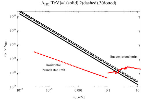
Figure 1: The line emission and horizontal branch star observation limits on the $s$. The region below the red-solid and - dashed lines are excluded. The data have been quoted from Refs. Baer:2014eja ; Mambrini:2015sia ; Raffelt:2006cw .

III.2.2 Constraints on the thermal $s$

The $s$-dark matter can be thermally produced by the scattering with the photon, $s+\gamma\leftrightarrow s+\gamma$, through the interaction in Eq.(64) with the coupling Eq.(65) in the early universe. The reaction rate $R(T)$ can roughly be estimated as

$$R(T)=n(T)\langle\sigma v\rangle\approx g_{s\gamma\gamma}^{4}T^{5}\,.$$ (69)

The decoupling temperature of the $s$, $T_{D}$, can be evaluated, by equating this $R(T)$ with the Hubble rate $H(T)\sim\sqrt{g_{*}(T)}T^{2}/M_{P}$ with the reduced Planck mass scale $M_{P}=2.44\times 10^{18}$ GeV and $g_{*}(T_{D})$ being the effective degrees of freedom for relativistic particles. The $g_{*}(T_{D})$ is estimated by combining the SM, the HC sector and the pseudoscalar $s$ as $g_{*}(T_{D})=g_{*}^{\rm SM}+g_{*}^{s}+g_{*}^{\rm HC}$, where $g_{*}^{\rm SM}=106.75$ Agashe:2014kda and $g_{*}^{s}=1$. The $g_{*}^{\rm HC}$ is calculated as

$$g_{*}^{\rm HC} = \left[2\times(N_{\rm HC}^{2}-1)\right]_{{\cal G}_{\rm HC}}+\frac{7}{8}N_{\rm HC}\left[(2\times 2\times 2)_{\chi}+(2\times 2)_{\psi}\right]$$ (70)

$$= 2(N_{\rm HC}^{2}-1)+\frac{21}{2}N_{\rm HC}\,.$$

For $N_{\rm HC}=(3,4,5)$, we have

$$g_{*}(T_{D})=(155.25,179.75,208.25)\,.$$ (71)

Thus we find

$$T_{D}\approx 10^{12}\,{\rm GeV}\times\left(\frac{3}{N_{\rm HC}}\right)^{2/3}\left(\frac{10^{-1}\,{\rm keV}}{m_{s}}\right)^{4/3}\left(\frac{\Lambda_{\rm HC}}{1\,{\rm TeV}}\right)^{8/3}\left(\frac{g_{*}(T_{D})}{200}\right)^{1/6}\,,$$ (72)

where Eq.(65) have been used.

Even after decoupling from the thermal equilibrium, the $s$ (with mass $\lesssim 1$ keV as in Eq.(68)) can be still relativistic at present, which is constrained by the null observation of dark radiations DiValentino:2016ikp . Since the $s$ goes cool down just like radiations due to the Hubble expansion after the decoupling, the present temperature of the $s$ is estimated as

$$T_{0}(s)=(t_{D}/t_{0})^{1/2}T_{D}=(g_{*}(T_{0})/g_{*}(T_{D}))^{1/4}T_{0}\simeq 10^{-4}{\rm eV}\,.$$ (73)

with $g_{*}(T_{0})=(2)_{\gamma}+(21/4(4/11)^{4/3})_{\nu}+(1)_{s}\simeq 4.36$. The current dark radiation constraint reads DiValentino:2016ikp $\Delta N_{\rm eff}=(T_{0}(s)/T_{0}(\nu))^{3}<0.1$ with $T_{0}(\nu)=(4/11)^{1/3}T_{0}$. The $s$ mass may thus be required to be

$$m_{s}\gtrsim 10^{-4}\,{\rm eV}\,.$$ (74)

If the $s$ decouples from the photon after the inflation and reheating temperature $T_{R}$, the temperature of the $s$ is heated back up to reach the same as the photon temperature, so that the $s$ would be a warm or hot dark matter-like particle. Currently such a light warm matter has been severely constrained by the cosmic microwave background spectrum. Hence we may escape from the case, by imposing $T_{D}>T_{R}$. The present model may follow a typical Higgs inflation scenario, as discussed in Ref. Reheating , in which $T_{R}\simeq 10^{14}$ GeV. Taking this value as a reference and using Eq.(72), we thus find

$$m_{s}\lesssim 1\,{\rm eV}\times\left(\frac{3}{N_{\rm HC}}\right)^{1/2}\left(\frac{\Lambda_{\rm HC}}{1\,{\rm TeV}}\right)^{2}\left(\frac{g_{*}(T_{D})}{200}\right)^{1/8}\,.$$ (75)

From Eqs.(68), (74) and (75), we thus see the $s$ mass constrained to be

$$10^{-4}\,{\rm eV}\lesssim m_{s}\lesssim 1\,{\rm eV}\,.$$ (76)

IV Cosmological productions and Detection of the $s$-dark matter

In this section, we closely explore the possibility for the $s$ as a dark matter to account for the relic abundance at the present time.

IV.1 Thermal production

Though the $s$-dark matter decouples from the thermal equilibrium in the early universe at $T_{D}\approx 10^{14}$ GeV $\times(1\,{\rm eV}/m_{s})^{4/3}(\gtrsim T_{R})$, there might exist the chance to thermally accumulate the number density by production cross sections interacting with the HC sector until the HC sector decouples from the thermal equilibrium at around $T=\Lambda_{\rm HC}={\cal O}({\rm TeV})$. The relevant production processes involve only a single $s$ in the final state through the $s-\gamma-\gamma$ vertex in Eq.(64) and the $s-Z-\gamma$, $s-Z-Z$ vertices listed in Appendix B, scattered off from the HC sector-fermion $F=(\chi,\psi)$ such as $F+\bar{F}\to\gamma/Z+s$. The production cross section roughly goes like

$$\sigma(F+\bar{F}\to\gamma/Z+s)\sim\alpha_{\rm em}N_{\rm HC}\left(\frac{\sqrt{N_{\rm HC}}g_{S}\alpha_{\rm em}}{\Lambda_{\rm HC}}\right)^{2}\simeq 10^{-31}\times\frac{N_{\rm HC}^{2}}{\Lambda_{\rm HC}^{2}}\left(\frac{m_{s}}{1\,{\rm eV}}\right)^{2}\left(\frac{1\,{\rm TeV}}{\Lambda_{\rm HC}}\right)^{2}\,,$$ (77)

where in the second equality we have used the first relationship in Eq.(63). The corresponding number density per entropy density at present time ($Y_{s}(T_{0})=n_{s}(T_{0})/s(T_{0})$) can be estimated by integrating the Boltzmann equation with the above production cross section over the temperature from the reheating temperature $T_{R}\approx 10^{14}$ GeV down to the freeze-out temperature $T_{F}=\Lambda_{\rm HC}$. Following the formula given in Ref. Choi:1999xm we thus evaluate the $Y_{s}(T_{0})$ as

$$Y_{s}(T_{0}) = \int_{\Lambda_{\rm HC}}^{T_{R}}dT\frac{\langle\sigma(F+\bar{F}\to\gamma/Z+s)v\rangle n_{F}n_{\bar{F}}}{s(T)H(T)T}\,$$ (78)

$$= \frac{135\sqrt{10}M_{P}}{2\pi^{3}}\int_{\Lambda_{\rm HC}}^{T_{R}}dT\frac{\langle\sigma(F+\bar{F}\to\gamma/Z+s)v\rangle n_{F}n_{\bar{F}}}{g_{*}^{3/2}(T)T^{6}}\,,$$

where in reaching the last line we used $H^{2}(T)=\frac{\pi^{2}}{30}g_{*}(T)T^{4}/(3M_{P}^{2})$, $s(T)=g_{s*}(T)\frac{2\pi^{2}}{45}T^{3}$, with $g_{*}(T)=g_{s*}(T)$ is assumed and the thermal average is expressed to be

$$\langle\sigma_{n}(F+\bar{F}\to s+\gamma/Z)v\rangle n_{F}n_{\bar{F}}=\zeta^{2}(3)\cdot\eta_{F}\eta_{\bar{F}}\cdot\frac{g_{F}g_{\bar{F}}}{16\pi^{4}}T^{6}\int_{0}^{\infty}dxx^{4}K_{1}(x)\sigma(x^{2})\,,$$ (79)

where $\zeta(3)=1.202...$ and $K_{1}(x)$ stands for the modified Bessel function of the first kind, $\sigma(x^{2})=\sigma(s/T^{2})$ and $g_{F(\bar{F})}$ is the internal (spin) degree of freedom for the HC fermion (anti-fermion) $F$; $\eta_{F(\bar{F})}$ is a number density factor associated with the initial state particle assigned as $\eta_{F}=3/4$ for fermions (anti-fermion). Using these we thus calculate the $Y_{s}(T_{0})$ to get

$$Y_{s}(T_{0}) \approx \frac{135\sqrt{10}}{32\pi^{6}}\frac{M_{P}T_{R}}{g_{*}^{3/2}(T_{R})\Lambda_{\rm HC}^{2}}\times 10^{-31}\times N_{\rm HC}^{2}\left(\frac{m_{s}}{1\,{\rm eV}}\right)^{2}\left(\frac{1\,{\rm TeV}}{\Lambda_{\rm HC}}\right)^{2}$$ (80)

$$\approx 10^{-10}\times N_{\rm HC}^{2}\left(\frac{m_{s}}{1\,{\rm eV}}\right)^{2}\left(\frac{1\,{\rm TeV}}{\Lambda_{\rm HC}}\right)^{4}\left(\frac{200}{g_{*}(T_{R})}\right)^{3/2}\,,$$

where use has been made of $g_{*}(T_{R})=g_{*}(\Lambda_{\rm HC})$. Thus, it turns out that the thermal relic is too small to explain the present dark matter abundance. This result is essentially tiled with the tiny coupling $g_{S}$ which leads to the extremely small cross section with the HC sector in Eq.(77).

IV.2 Non-thermal production

Analogously to the case of axion dark matter Baer:2014eja , the $s$-dark matter population can be accumulated by “misalignment” of the classical $s$ field and the coherent oscillation. Assuming the initial position at which the oscillation starts to be the vicinity of the vacuum $s=0$ with the vacuum expectation value $v_{S}$, we write the equation of motion for the $s$ under the Friedmann-Robertson-Walker metric to be

$$\frac{d^{2}s}{dt^{2}}+3H(T)\frac{ds}{dt}+m_{s}^{2}\,s\approx 0\,.$$ (81)

This describes the damping harmonic oscillation in which the oscillation takes place when $T=T_{\rm osc}$ where $3H(T)\approx m_{s}$, i.e.,

$$T_{\rm osc}\simeq 13\,{\rm TeV}\times\left(\frac{m_{s}}{1\,\rm eV}\right)^{1/2}\left(\frac{200}{g_{*}(T_{\rm osc})}\right)^{1/4}\,.$$ (82)

This implies that $130\,{\rm GeV}\lesssim T_{\rm osc}\lesssim 13$ TeV for $10^{-4}\,{\rm eV}\lesssim m_{s}\lesssim 1$ eV. Since the $s$ mass is generated through the bosonic seesaw at $T\simeq\Lambda_{\rm HC}={\cal O}(1)$ TeV, we find that the temperature at which the coherent oscillation starts, what we call $T_{S}$, depend on the $m_{s}$ as

$$T_{S} \simeq \Lambda_{\rm HC}\,\qquad{\rm for}\qquad 6\times 10^{-3}\,{\rm eV}\left(\frac{\Lambda_{\rm HC}}{1\,{\rm TeV}}\right)^{2}\lesssim m_{s}<1\,{\rm eV}\,,$$

$$T_{S} \simeq T_{\rm osc}\,\qquad{\rm for}\qquad 10^{-4}\,{\rm eV}\lesssim m_{s}\lesssim 6\times 10^{-3}\,{\rm eV}\left(\frac{\Lambda_{\rm HC}}{1\,{\rm TeV}}\right)^{2}\,.$$ (83)

The energy density of the classical $s$ field is thus accumulated by the coherent oscillation starting from the temperature $T_{S}$ in Eq.(83), cooling down to the present temperature $T_{0}$.

At the $T=T_{S}$ the energy density of the $s$ corresponds to the vacuum energy defined as

$$\rho_{s}(T_{S})=V(\theta)-V(\theta=0)\,,$$ (84)

where the $\theta$ is defined as the amount of the shift from the original $S$ field at the vacuum expectation value $v_{S}$ to be $S=v_{S}(1+\theta)$ with $\theta\ll 1$, and the potential $V(\theta)$ is read off as

$$V(\theta)=V(\theta=0)+\frac{1}{2}m_{s}^{2}v_{s}^{2}\theta^{2}+{\cal O}(\theta^{3})\,.$$ (85)

One can easily see that during the coherent oscillation, the number density per comoving volume is conserved and the $s$ behaves just like a non-relativistic particle satisfying $\rho_{s}\propto R^{-3}$ with the expansion rate $R$. Hence we write

$$\frac{\rho_{s}(T_{S})}{\rho_{s}(T_{0})}=\frac{m_{s}n_{s}(T_{S})}{m_{s}n_{s}(T_{0})}=\frac{s(T_{S})}{s(T_{0})}\,,\qquad{\rm i.e.,}\qquad\rho_{s}(T_{0})=\frac{s(T_{0})}{s(T_{S})}\rho_{s}(T_{S})\,.$$ (86)

Thus, we get the present abundance of DM as

$$\rho_{s}(T_{0})\simeq(4200~{}{\rm GeV})^{4}\left(\frac{T_{0}}{T_{S}}\right)^{3}\frac{g_{\ast S}(T_{0})}{g_{\ast S}(T_{S})}\theta^{2}\left(\frac{m_{\Pi}}{750~{}{\rm GeV}}\right)^{2}\left(\frac{\Lambda_{\rm HC}}{1~{}{\rm TeV}}\right),$$ (87)

by using Eqs. (63). This relation shows that we can explain the correct abundance of $s$ with an appropriate value of $\theta$ even when the HC pion mass is heavier/lighter than $750$ GeV.

From Eqs.(83), (85) and (86), and using the second equality in Eq.(63), we thus estimate the $s$-dark mater relic density, $\Omega_{s}h^{2}=\rho_{s}(T_{0})/(\rho_{\rm cr}/h^{2})$ with $\rho_{\rm cr}/h^{2}=0.8\times 10^{-46}\,{\rm GeV}^{4}$. The contour plot on the $(m_{s},\theta)$ plane with the observed dark matter relic density $\Omega_{\rm DM}h^{2}\simeq 0.118$ Agashe:2014kda has been drawn in Fig. 2. Here use has been made of $s(T_{0})=\frac{2\pi^{2}}{45}g_{s*}(T_{0})T_{0}^{3}$ with $g_{*s}(T_{0})=43/11$ and $T_{0}\simeq 2.4\times 10^{-4}$ eV, $g_{s*}(\Lambda_{\rm HC})=200$ taken as a reference value, and we have assumed $g_{s*}(T_{S}<\Lambda_{\rm HC})=g_{*}^{\rm SM}=106.75$. From the figure, we find that the relic density of the $s$, with the mass in a range of $10^{-4}\,{\rm eV}\lesssim m_{s}\lesssim 1\,{\rm eV}$, can be accumulated enough to account for the present dark matter abundance.

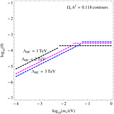
Figure 2: The contour plots on the $(m_{s},\theta)$ plane realizing the observed present dark matter density $\Omega_{\rm DM}h^{2}=0.118$ Agashe:2014kda . The bumps, which show up when $T_{S}$ gets lower than $\Lambda_{\rm HC}$, are due to the discontinuity of the effective degrees of freedom $g_{s*}$ around the $T_{S}=\Lambda_{\rm HC}$ as described in the text.

IV.3 Detection possibility in experiments

As has so far been seen in this section, the $s$-dark matter has the lifetime much longer than the age of the universe and has extremely tiny couplings to the SM particles, and hence the detection at collider experiments is unlikely to be possible.

As in the case of invisible axion-like dark matter detection SikivieDetection , cosmic pseudoscalar $s$, left over from the big bang, may be detected by microwave cavity haloscopes. In that facility, a strong static magnetic field is provided to make the $s$ drift through the microwave cavity, resonantly converted to microwave photons according to the $s$-photon-photon interaction in Eq.(64). The conversion power $P$ is given by SikivieDetection

$$P=\frac{1}{8}g_{s\gamma\gamma}^{2}\rho_{s}(T_{0})B_{0}^{2}L_{x}V\,,$$ (88)

where $\rho_{s}(T^{0})$ is the local $s$ energy density, $B_{0}$ the magnetic strength scale, $V$ the volume of the cavity and $L_{x}$ the size of the $x$ direction. Taking a typical experimental setup currently employed Bradley:2003kg , $B_{0}=10\,{\rm Tesla},$ $L_{x}=1\,{\rm m}$, $V=1\,{\rm m}^{3}$ and the local halo density $\rho_{\rm halo}\simeq 0.3\,{\rm GeV}/{\rm cm}^{3}$, we estimate the detection power

$$P/N_{\rm HC}\simeq 10^{-34}\,{\rm Watt}\times\left(\frac{1\,{\rm TeV}}{\Lambda_{\rm HC}}\right)^{2}\left(\frac{m_{s}}{10^{-4}\,{\rm eV}}\right)^{2}\left(\frac{\rho_{s}(T_{0})}{\rho_{\rm halo}}\right)\,,$$ (89)

where we have used Eq.(65). The power for $m_{s}\sim 1$ eV is comparable with the axion detection potential Bradley:2003kg , so the $s$ can be hunted at the same level of the sensitivity as the axion by the microwave cavity experiments.

V Summary and Discussion

In this paper, we have employed a model based on the classically-scale invariant standard model extended by adding a strongly coupled hypercolor dynamics. The dynamical breaking of the scale symmetry is triggered by the vector-like condensation at the TeV scale, so that the standard model Higgs acquires the negative mass-squared by the bosonic seesaw mechanism to realize the electroweak symmetry breaking.

What is significant to control this model is to include an elementary pseudoscalar $S$, which plays the crucial role to realize the electroweak bosonic seesaw, as well as to give masses for the composite Nambu-Goldstone bosons (hypercolor pions): in this sense, the $S$ acts like another “Higgs” in the theory. Thus, discovering the fluctuating mode of $S$, called $s$, is the smoking-gun of the present model.

Because of the classical-scale invariance, the pseudoscalar $S$ originally couples only to the standard model Higgs and hypercolor fermions. After the dynamical-scale breaking and triggering the electroweak bosonic seesaw, the $s$ thus develops vanishingly small couplings to the standard model particles, which arise only through the tiny mixing with the hypercolor eta-prime. In addition, it turned out that in relation to the hypercolor pion masses the $s$ mass is predicted to be very light and to predominantly decay to diphoton, so we have identified the $s$ as a dark matter candidate. The $s$ mass was then severely constrained by several cosmological observations, such as line emissions of X-ray, gamma-ray and cosmic-ray, no evidence for dark radiations, and a typical Higgs inflation scenario. The $s$ mass was thus bounded to be $10^{-4}{\rm eV}\lesssim m_{s}\lesssim 1{\rm eV}$.

We examined the possibility of the cosmological productions of the $s$. It was shown that the $s$ is unlikely to be thermally produced essentially due to its tiny couplings to the hypercolor sector in the thermal equilibrium. We then found that the sufficient amount of relic abundance of $s$ as the cold dark matter can be accumulated via the coherent oscillation.

The detection potential in microwave cavity experiments was also addressed so that the $s$ with mass around 1 eV can have the same level of the detection sensibility as that of the axion in the currently equipped experimental setup, so the $s$ can be hunted by the microwave cavity experiments.

Several comments are in order:

The crucial deference between the $s$-dark matter and the axion-like dark matter can be seen by no evidence for observations probing couplings to matter, such as the test of gravitational inverse-square law and energy loss in stars like neutron star cooling. The $s$ coupling to matters can be generated at loop levels by the $g_{S}$ and $\kappa_{H}$ couplings. As seen from Eqs.(57) and (58), however, those couplings are extremely small, suppressed by $(m_{s}/\Lambda)\ll 1$ or $(v_{1}/v_{s})\ll 1$ (See also Eq.(62)). Hence one can conclude that there is no chance to detect the $s$-dark matter through the couplings to matters, in contrast to the axion case. Thus, no evidence for observations with the matter-portal, but some signals identical among the $s$ and the axion in the line shapes and microwave cavity experiments would be a clear hint to distinguish them. (Note that a dilaton-like dark matter signal in the microwave cavity is clearly different from that of the $s$ and the axion, due to the different type of the coupling to photons: $E\cdot B$ for pseudoscalars, while $E\cdot E$ or $B\cdot B$ for scalars.)

As discussed in Secs. III and IV, we have assumed that the reheating epoch is associated with the Higgs inflation scenario. It might be the case, however, that one needs somewhat large non-minimal couplings between the SM Higgs and the scalar curvature for the reheating temperature in the Higgs inflation scenario. In that case, the reheating epoch would be shifted, so the upper bound on the mass of $s$, as estimated in Eq. (75), could be affected. Detailed study closely connected with inflation scenarios is to be performed in the future literature.

The predicted number in Eq.(89) depends on the $s$ mass, so it does also on the hypercolor pion mass through Eq.(63). It should be noted, however, that the light pseudoscalar $s$ as a candidate of the dark matter is intact even if the hypercolor pion mass is not set to the present reference value, since it is solely tied with realization of the electroweak breaking via the bosonic seesaw: the mass has to be much smaller than $\Lambda_{\rm HC}$, which is controlled by the small coupling $g_{S}(\ll 1)$ in Eq.(58); the $s$ couplings to the standard model particles, photons, necessarily becomes tiny by the same $g_{S}$ coupling strength as the consequence of the bosonic seesaw, which would suggest to regard the $s$ as a dark matter candidate; the $s$ mass is then inevitably constrained by cosmological bounds, to be order of eV, as was discussed in the text.

Actually, the couplings of the s-dark matter are required to be extremely small: the coupling to hyperfermion, $g_{S}\sim 10^{-12}$, from Eq. (63) for $m_{s}\sim 1{\rm eV}$ (which is coincidentally as small as the Yukawa coupling for neutrino in Dirac neutrino models); the quartic coupling $\lambda_{S}\sim 10^{-44}$ from Eq. (58) with $v_{S}\sim 10^{13}$ GeV estimated from Eq. (62) with $m_{s}\sim 1{\rm eV}$ and $g_{S}\sim 10^{-12}$; the coupling to the 125 GeV Higgs, $\kappa_{H}\sim 10^{-22}$, estimated from Eq. (58) with $v_{S}\sim 10^{13}$ GeV. The origin of these extremely small couplings could be explained by the underlying Planck scale physics, which is, however, beyond the scope of the present study, to be pursued elsewhere. Note that the realization of the electroweak symmetry breaking has nothing theoretically to do with the smallness of those coupling parameters, which are only related to the physics of the light $s$ including the mass generation of hypercolor pions and the property as the invisible dark matter.

Other signals characteristic to the present model involve not only hypercolor pions, but also the hypercolor eta-prime and hypercolor composite scalar states, both of which are expected to have the mass on the order of $\Lambda_{\rm HC}$. As briefly studied in Appendix C, the hypercolor eta-prime can be produced at the LHC, via the photon - photon fusion process as well as the hypercolor pions. The discovery channels will be similar to the hypercolor pions: $WW,ZZ,Z\gamma$ and $\gamma\gamma$ modes. Since the production cross section decreases as the resonance mass grows, the photon - photon fusion cross section for the hypercolor eta-prime significantly gets smaller than that of the hypercolor pions, so it may be challenging to search at the LHC (For explicit estimates for the signal strengths, see Appendix C).

As to the hypercolor composite scalars, the couplings to the standard model particles are controlled by the tiny Yukawa coupling $y(\ll 1)$ through the mixing with the standard model Higgs. It would be worth investigating how much large the $y$ coupling is allowed to be consistent with the currently reported heavy Higgs search data, and to discuss the LHC discovery potential. Such those topics are deserved to the future study.

In closing, in the present work we have so far focused on the possibility for the predicted light pseudoscalar $s$ to be a dark matter candidate. Actually, another scenario can be made: with the $s$ mass around GeV scale the $s$ could be just a long-lived particle having the lifetime much shorter than the age of the present universe. That sort of a light long-lived particle could be accessible at the LHC. This interesting another possibility will be pursued in another publication.

Appendix A Computation of HC pion masses

In this Appendix we shall calculate the HC pion masses arising from the $g_{S}$ and $y$ terms in Eqs.(7) and (6).

A.1 Masses from the $g_{S}$ term

First of all, one should note that the nonzero vacuum expectation value of $S$, $v_{S}$, is required in the present model, which provides masses for the 8 HC pions $(\Pi^{a})$ via the $g_{S}$ term in Eq.(7). The HC pion masses can be evaluated according to the standard current algebra, which turn out to show up at the second order of perturbation in $g_{S}$:

$$(m_{\Pi}^{2})^{ab}\Bigg{|}_{g_{S}}=-\frac{i}{2}g_{S}^{2}v_{S}^{2}\int d^{4}x\langle\Pi^{a}|T(J_{P}(x)J_{P}(0))|\Pi^{b}\rangle\,,$$ (90)

where $J_{P}(x)=i\bar{F}(x)\gamma_{5}F(x)$ and the symbol “$T$” stands for the time-ordered product. We use the partially-conserved axialvector current (PCAC) relations and the current algebra,

$$\partial^{\mu}J_{\mu 5}^{a}(x)=-f_{\Pi}m_{\Pi}^{2}\,\Pi^{a}(x)\,,$$

$$[iQ_{5}^{a},{\cal O}(x)]=\delta^{a}_{5}{\cal O}(x)\,,\qquad Q_{5}^{a}=\int d^{3}xJ_{5}^{0}(x)\,,$$ (91)

where the current $J_{\mu 5}^{a}$ is defined as $J_{\mu 5}^{a}=\bar{F}\gamma_{\mu}\gamma_{5}(\lambda^{a}/2)F$ with the generator $(\lambda^{a}/2)$ with the Gell-Mann matrix $\lambda^{a}$ ($a=1,\cdots 8$); $f_{\Pi}$ is the $\Pi$-decay constant, defined as $\langle 0|J_{\mu}^{a}(0)|\Pi^{b}(p)\rangle=-ip_{\mu}f_{\Pi}\delta^{ab}$; the ${\cal O}$ denotes an arbitrary Heisenberg operator, and $\delta^{a}_{5}$ denotes the infinitesimal-“chiral” transformation, which acts on the $F$-fermion as $\delta^{a}_{5}F=-i\gamma_{5}(\lambda^{a}/2)F$. Using these together with the reduction formula, one thus evaluates Eq.(90) to arrive at

$$(m_{\Pi}^{2})^{ab}\Bigg{|}_{g_{S}} = m_{\Pi}^{2}\,=-4i\frac{g_{S}^{2}v_{S}^{2}}{f_{\Pi}^{2}}\,\delta^{ab}\,\int d^{4}x\left(\langle 0|T(J_{S}^{a}(x)J_{S}^{b}(0))|0\rangle-\langle 0|T(J_{\eta^{\prime}}(x)J_{\eta^{\prime}}(0))|0\rangle\delta^{ab}\right)$$ (92)

$$= 4\frac{g_{S}^{2}v_{S}^{2}}{f_{\Pi}^{2}}\,\delta^{ab}\,\left[\Pi_{S}(0)-\Pi_{\eta^{\prime}}(0)\right]\,,$$

where $J_{S}^{a}(x)=\bar{F}(x)(\lambda^{a}/2)F(x),J_{\eta^{\prime}}(x)=\frac{1}{\sqrt{6}}\bar{F}(x)i\gamma_{5}F(x)$ and we have defined the current correlators $\Pi_{S,\eta^{\prime}}$ as

$$\,\int d^{4}xe^{ipx}\langle 0|T(J_{S}^{a}(x)J_{S}^{b}(0))|0\rangle \equiv i\Pi_{S}(p^{2})\delta^{ab}\,$$

$$\,\int d^{4}xe^{ipx}\langle 0|T(J_{\eta^{\prime}}(x)J_{\eta^{\prime}}(0))|0\rangle \equiv i\Pi_{\eta^{\prime}}(p^{2})\,.$$ (93)

We may expand the correlators by assuming the resonances pole saturation,

$$\Pi_{S}(p^{2}) = \sum_{n=1}^{\infty}\frac{F_{S_{n}}^{2}m_{S_{n}}^{2}}{m_{S_{n}}^{2}-p^{2}}\,,$$

$$\Pi_{\eta^{\prime}}(p^{2}) = \sum_{n=1}^{\infty}\frac{F_{\eta_{n}^{\prime}}^{2}m_{\eta_{n}^{\prime}}^{2}}{m_{\eta^{\prime}_{n}}^{2}-p^{2}}\,,$$ (94)

with the masses $(m_{S_{n}},m_{\eta^{\prime}_{n}})$ and the decay constants $(F_{S_{n}},F_{\eta^{\prime}_{n}})$. Then the HC pion mass formula in Eq.(92) is rewritten as a sum rule to be

$$m_{\Pi}^{2}\Bigg{|}_{g_{S}}=4\frac{g_{S}^{2}v_{S}^{2}}{f_{\Pi}^{2}}\sum_{n}\left[F_{S_{n}}^{2}-F_{\eta_{n}^{\prime}}^{2}\right]\,.$$ (95)

Analogously to the QCD case, the $\eta^{\prime}\equiv\eta^{\prime}_{(n=1)}$ decay constant $F_{\eta^{\prime}_{1}}$ is expected to be of order of the pion decay constant Gasser:1984gg , $f_{\Pi}\sim{\cal O}(\frac{\Lambda_{\rm HC}}{4\pi})$, and the higher resonance contributions could numerically be cancelled each other in the sum between the scalar and pseudoscalar sector, namely, by $F_{S_{n}}\simeq F_{\eta^{\prime}_{n}}\simeq{\cal O}(\Lambda_{\rm HC})$ for $n\geq 2$. Thus we may evaluate the sum rule just by keeping the lowest resonance contribution:

$$m_{\Pi}^{2}\Bigg{|}_{g_{S}} \simeq 4\frac{g_{S}^{2}v_{S}^{2}}{f_{\Pi}^{2}}\left(F_{S_{1}}^{2}-F_{\eta^{\prime}_{1}}^{2}\right)$$ (96)

$$\simeq 4\frac{g_{S}^{2}v_{S}^{2}}{f_{\Pi}^{2}/(N_{\rm HC}/3)}\Lambda_{\rm HC}^{2}\,,$$

where in the last line we have clarified that the mass is independent of the number of HC, $N_{\rm HC}$.

Thus the derivation of Eq.(59) has been compensated.

A.2 Masses from the $y$-term

Similarly to the $g_{S}$ term, the $y$-Yukawa term (${\cal L}_{y}$) in Eq.(6) gives masses to the HC pions via the $H$-Higgs vacuum expectation value $v_{1}\simeq 246$ GeV. Again, the estimate of the mass can be done by using the current algebra technique:

$$(m_{\Pi}^{2})^{ab}\Bigg{|}_{y} = -\frac{1}{f_{\Pi}^{2}}\langle 0|[iQ_{5}^{a},[iQ_{5}^{b},{\cal L}_{y}]]|0\rangle$$ (97)

$$= -\frac{yv_{1}}{\sqrt{2}f_{\Pi}^{2}}\langle 0|[iQ_{5}^{a},[iQ_{5}^{b},\bar{\chi}_{2}\psi+\bar{\psi}\chi_{2}]]|0\rangle\,.$$

The nonzero elements for the mass matrix are thus found be

$$(m_{\Pi}^{2})^{14}\Bigg{|}_{y} = (m_{\Pi}^{2})^{14}\Bigg{|}_{y}=-\frac{yv_{1}}{f_{\Pi}^{2}}\langle\bar{F}F\rangle\,,\qquad(m_{\Pi}^{2})^{25}\Bigg{|}_{y}=(m_{\Pi}^{2})^{52}\Bigg{|}_{y}=-\frac{yv_{1}}{f_{\Pi}^{2}}\langle\bar{F}F\rangle\,,$$

$$(m_{\Pi}^{2})^{36}\Bigg{|}_{y} = (m_{\Pi}^{2})^{63}\Bigg{|}_{y}=\frac{yv_{1}}{f_{\Pi}^{2}}\langle\bar{F}F\rangle\,,\qquad(m_{\Pi}^{2})^{68}\Bigg{|}_{y}=(m_{\Pi}^{2})^{86}\Bigg{|}_{y}=\sqrt{3}\frac{yv_{1}}{f_{\Pi}^{2}}\langle\bar{F}F\rangle\,,$$ (98)

where $\langle\bar{F}F\rangle$ denotes the “chiral” condensate per flavors, i.e., $\langle\bar{F}F\rangle=\langle\bar{\chi}_{1}\chi_{1}\rangle=\langle\bar{\chi}_{2}\chi_{2}\rangle=\langle\bar{\psi}\psi\rangle$.

A.3 Diagonalization of the HC pion sector

Combining Eqs.(96) with Eq.(98). one finds the HC pion mass matrix acting on the current-eigenstate vector $(\Pi^{1},\cdots,\Pi^{8})^{T}$:

$$\left(\begin{array}[]{c|c|c|c|c|c|c|c}m^{2}_{g_{S}}&0&0&(m^{2}_{y})^{14}&0&0&0&0\\ \hline\cr 0&m^{2}_{g_{S}}&0&0&(m^{2}_{y})^{25}&0&0&0\\ \hline\cr 0&0&m^{2}_{g_{S}}&0&0&(m^{2}_{y})^{36}&0&0\\ \hline\cr(m^{2}_{y})^{41}&0&0&m^{2}_{g_{S}}&0&0&0&0\\ \hline\cr 0&(m^{2}_{y})^{52}&0&0&m^{2}_{g_{S}}&0&0&0\\ \hline\cr 0&0&(m^{2}_{y})^{63}&0&0&m^{2}_{g_{S}}&0&(m^{2}_{y})^{68}\\ \hline\cr 0&0&0&0&0&0&m^{2}_{g_{S}}&0\\ \hline\cr 0&0&0&0&0&(m^{2}_{y})^{86}&0&m^{2}_{g_{S}}\\ \end{array}\right)\,,$$ (107)

where $m^{2}_{g_{S}}$ and $(m_{y}^{2})^{ab}$ respectively stand for the masses in Eqs.(96) and (98). The mass matrix can easily be diagonalized by an orthogonal rotation, which relates the current eigenstates $\{\Pi\}$ with the mass eigenstates $\{\tilde{\Pi}\}$ as

$$\left(\begin{array}[]{cc}\tilde{\Pi}^{1}\\ \tilde{\Pi}^{4}\end{array}\right) = \left(\begin{array}[]{cc}-\frac{1}{\sqrt{2}}&\frac{1}{\sqrt{2}}\\ \frac{1}{\sqrt{2}}&\frac{1}{\sqrt{2}}\end{array}\right)\left(\begin{array}[]{cc}{\Pi}^{1}\\ {\Pi}^{4}\end{array}\right)\,,$$ (114)

$$\left(\begin{array}[]{cc}\tilde{\Pi}^{2}\\ \tilde{\Pi}^{5}\end{array}\right) = \left(\begin{array}[]{cc}-\frac{1}{\sqrt{2}}&\frac{1}{\sqrt{2}}\\ \frac{1}{\sqrt{2}}&\frac{1}{\sqrt{2}}\end{array}\right)\left(\begin{array}[]{cc}{\Pi}^{2}\\ {\Pi}^{5}\end{array}\right)\,,$$ (121)

$$\left(\begin{array}[]{cc}\tilde{\Pi}^{3}\\ \tilde{\Pi}^{6}\\ \tilde{\Pi}^{8}\end{array}\right) = \left(\begin{array}[]{ccc}-\frac{\sqrt{3}}{\sqrt{2}}&0&\frac{1}{2}\\ \frac{1}{2\sqrt{2}}&-\frac{1}{\sqrt{2}}&\frac{1}{2}\sqrt{\frac{3}{2}}\\ \frac{1}{2\sqrt{2}}&\frac{1}{\sqrt{2}}&\frac{1}{2}\sqrt{\frac{3}{2}}\end{array}\right)\left(\begin{array}[]{cc}{\Pi}^{3}\\ {\Pi}^{6}\\ {\Pi}^{8}\end{array}\right)\,,$$ (131)

$$\tilde{\Pi}^{7} = \Pi^{7}\,,$$ (132)

with the mass eigenvalues,

$$m_{\tilde{\Pi}^{1}}^{2} = m_{\tilde{\Pi}^{2}}^{2}\simeq m_{g_{S}}^{2}+\frac{yv_{1}\langle\bar{F}F\rangle}{\sqrt{2}f_{\Pi}^{2}}\,,$$

$$m_{\tilde{\Pi}^{3}}^{2} \simeq m_{g_{S}}^{2}\,,$$

$$m_{\tilde{\Pi}^{4}}^{2} = m_{\tilde{\Pi}^{5}}^{2}\simeq m_{g_{S}}^{2}-\frac{yv_{1}\langle\bar{F}F\rangle}{\sqrt{2}f_{\Pi}^{2}}\,,$$

$$m_{\tilde{\Pi}^{6}}^{2} \simeq m_{g_{S}}^{2}-\frac{\sqrt{2}yv_{1}\langle\bar{F}F\rangle}{f_{\Pi}^{2}}\,,$$

$$m_{\tilde{\Pi}^{7}}^{2} \simeq m_{g_{S}}^{2}\,,$$

$$m_{\tilde{\Pi}^{8}}^{2} \simeq m_{g_{S}}^{2}+\frac{\sqrt{2}yv_{1}\langle\bar{F}F\rangle}{f_{\Pi}^{2}}\,,$$ (133)

where terms of ${\cal O}(y^{2})$ have been neglected.

By tuning $y$ to be $\ll 1$, we may thus neglect the $y$-corrections to the HC pion masses. Note that even if those off-diagonal corrections are numerically neglected, the HC pions significantly mix independently of the $y$ as in Eq.(132): this is the reflection of degenerate perturbation theory well-known in the quantum mechanics. Such a “non-decoupling” mixing will thus affect the HC pion phenomenology as described in the next Appendices.

Appendix B Effective “Chiral” Lagrangian

In this Appendix we present the effective “chiral” Lagrangian for the HC pions and derive interaction terms relevant to study the LHC phenomenology.

The low-energy effective theory of the present model can be described by the HC pion fields $\Pi$, by the nonlinear realization of the underlying flavor “chiral” $SU(3)_{L}\times SU(3)_{R}$ symmetry associated with the flavor condensate of $F$-fermions $F_{L,R}=(\chi_{i},\psi)_{L,R}$ ($i=1,2$), $\langle\bar{\chi}_{i}\chi_{i}\rangle=\langle\bar{\psi}\psi\rangle\neq 0$. The basic variable to construct the effective model is the “chiral” field $U$, which transforms under the global “chiral” symmetry as $U\to g_{L}\cdot U\cdot g_{R}^{\dagger}$, where $g_{L,R}$ belong to the “chiral” $SU(3)_{L,R}$ groups, respectively. When the SM gauges are turned on, the global “chiral” symmetry is partially localized according to the SM-gauge embedding as in Ref. Haba:2015qbz . Then the effective gauged-“chiral” Lagrangian invariant under the chiral $SU(3)_{L}\times SU(3)_{R}$ and $U(1)_{V}$ symmetries is written as

$${\cal L}_{\rm eff} = {\cal L}_{\rm kin}+{\cal L}_{\rm mass}+\cdots$$

$${\cal L}_{\rm kin} = \frac{f_{\Pi}^{2}}{4}{\rm tr}[|D_{\mu}U|^{2}]$$

$${\cal L}_{\rm mass} = b\,{\rm tr}[U{\cal M}^{\dagger}+{\rm h.c.}]\,,$$ (134)

where

$$U = \exp\left({\frac{2i\Pi}{f_{\Pi}}}\right)=\exp\left({\frac{2i\sum_{a=1}^{8}\Pi^{a}\frac{\lambda^{a}}{2}}{f_{\Pi}}}\right)\,,$$

$$D_{\mu}U = \partial_{\mu}U-i[{\cal V}_{\mu},U]\,,$$

$${\cal V}_{\mu} = g_{W}W_{\mu}+g_{Y}B_{\mu}=g_{W}\sum_{a=1}^{3}W_{\mu}^{a}\frac{\lambda^{a}}{2}+g_{Y}B_{\mu}Y_{F}\,,$$

$$Y_{F} = \frac{\sqrt{3}}{6}\lambda_{8}+\frac{1}{\sqrt{6}}\lambda_{0}=\left(\begin{array}[]{ccc}1&&\\ &1&\\ &&0\end{array}\right)\,,\qquad\lambda_{0}=\frac{2}{\sqrt{6}}{\bf 1}_{3\times 3}\,,$$ (138)

with $\lambda^{a}$ $(a=1,\cdots,8)$ being the Gell-Mann matrices normalized as ${\rm tr}[\lambda^{a}\lambda^{b}]=2\delta_{ab}$, $(W_{\mu}^{a},B_{\mu})$ the electroweak gauge fields in the SM, and $U$ parametrizes the HC pion fields with regard to the spontaneous breaking of the “chiral” $SU(3)_{L}\times SU(3)_{R}$ symmetry down to the diagonal subgroup $SU(3)_{V}$, just like the ordinary QCD, with the associated HC pion decay constant $f_{\Pi}$. The electroweak charges of $U$ have come from the underlying $F$-fermion fields and its vector-like condensate Haba:2015qbz . In Eq.(134) two spurion field ${\cal M}$ has been introduced, in which ${\cal M}$ transforms under the “chiral” in the same as $U$ (${\cal M}\to g_{L}\cdot{\cal M}\cdot g_{R}^{\dagger}$). The spurion field is assumed to get the vacuum expectation value, $\langle{\cal M}\rangle={\bf 1}_{3\times 3}$. leading to the explicit breaking of the “chiral” symmetry. Then, the ${\cal L}_{\rm mass}$ term can be matched to the underlying explicit breaking term, as discussed in the previous section, to determine the parameter $b$ in front of it. The explicit relation between the parameter $b$ and those explicit breaking coefficients will be irrelevant for the present study, so will not be specified here.

In addition to the Lagrangian in Eq.(134), the HC sector yields anomalous vertices related to the “chiral” $SU(3)_{L}\times SU(3)_{R}$ anomaly with the SM charges gauged, a la Wess-Zumino-Witten term Wess:1971yu . Such terms give significant contributions to HC pion decays to dibosons involving photons. Taking into account the fact that only vectorial symmetry has been gauged at present, one easily finds that only the following term is relevant for the diboson processes:

$${\cal L}_{\rm WZW}=-\frac{N_{\rm HC}}{4\pi^{2}f_{\Pi}}\epsilon^{\mu\nu\rho\sigma}{\rm tr}[\partial_{\mu}{\cal V}_{\nu}\partial_{\rho}{\cal V}_{\sigma}\Pi]\,.$$ (139)

The SM gauge fields in the mass basis $(W^{\pm}_{\mu},Z_{\mu},A_{\mu})$ can be encoded there, by the standard manipulation with Eq.(134) as

$$W_{\mu}^{\pm} = \frac{W_{\mu}^{1}\mp iW_{\mu}^{2}}{\sqrt{2}}\,,$$

$$W^{3}_{\mu} = c_{W}Z_{\mu}+s_{W}A_{\mu}\,,\qquad B_{\mu}=-s_{W}Z_{\mu}+c_{W}A_{\mu}\,,$$

$$s_{W} \equiv \frac{g_{Y}}{\sqrt{g_{W}^{2}+g_{Y}^{2}}}\,,\qquad c_{W}^{2}\equiv 1-s_{W}^{2}\,.$$ (140)

in which the electromagnetic coupling $e$ is written as $1/e^{2}=1/g_{W}^{2}+1/g_{Y}^{2}$. In terms of the mass-eigenstate gauge fields $(W_{\mu}^{\pm},A_{\mu},Z_{\mu})$, the external gauge field ${\cal V}_{\mu}$ is expressed as

$${\cal V}_{\mu} = \frac{e}{\sqrt{2}s_{W}}\left(W_{\mu}^{+}I^{+}+W_{\mu}^{-}I^{-}\right)$$ (141)

$$+eQ_{\rm em}^{F}A_{\mu}+\frac{e}{s_{W}c_{W}}\left(I^{3}-s_{W}^{2}Q_{\rm em}^{F}\right)Z_{\mu}\,,$$

where

$$I^{3} = \frac{\lambda^{3}}{2}\,,\qquad I^{\pm}=\frac{\lambda^{1}\pm i\lambda^{2}}{2}\,,$$

$$Q_{\rm em}^{F} = I^{3}+Y_{F}=\left(\begin{array}[]{ccc}1&&\\ &0&\\ &&0\end{array}\right)\,,$$ (145)

Expanding the $\Pi$ field parametrized as in Eq.(138) in terms of the component fields $\Pi^{a}$ $(a=1,\cdots,8)$, and using Eq.(141), one readily finds that the couplings to neutral $\Pi$’s arise as follows:

$${\cal L}_{\rm WZW}^{\rm NC} = -\frac{N_{\rm HC}}{4\pi^{2}f_{\Pi}}\sum_{a=3,6,8}\Bigg{[}{\rm tr}[I^{a}\{I^{+},I^{-}\}]\cdot\frac{e^{2}}{2s_{W}^{2}}dW^{+}dW^{-}\Pi^{a}+{\rm tr}[I^{a}\{Q_{\rm em}^{F},I^{3}-s_{W}^{2}Q_{\rm em}^{F}\}]\cdot\frac{e^{2}}{s_{W}c_{W}}dAdZ\Pi^{a}$$ (146)

$$+{\rm tr}[I^{a}Q_{\rm em}^{F}Q_{\rm em}^{F}]\cdot e^{2}dAdA\Pi^{a}-{\rm tr}[I^{a}\left(\{I^{3},Q_{\rm em}^{F}\}-s_{W}^{2}\cdot Q_{\rm em}^{F}Q_{\rm em}^{F}\right)]\ \cdot\frac{e^{2}}{c_{W}^{2}}dZdZ\Pi^{a}\Bigg{]}$$

$$= -\frac{N_{\rm HC}}{4\pi^{2}f_{\Pi}}\left[\frac{e^{2}}{2}dAdA+\frac{e^{2}(c_{W}^{2}-s_{W}^{2})}{2s_{W}c_{W}}dAdZ-\frac{e^{2}}{2}dZdZ\right]\left(\Pi^{3}+\frac{\Pi^{8}}{\sqrt{3}}\right)$$

$$-\frac{N_{\rm HC}}{4\pi^{2}f_{\Pi}}\left[\frac{e^{2}}{2s_{W}^{2}}dW^{+}dW^{-}\right]\left(\frac{\Pi^{8}}{\sqrt{3}}\right)\,,$$

where $dV_{1}dV_{2}\equiv\epsilon^{\mu\nu\rho\sigma}\partial_{\mu}V_{1\nu}\partial_{\rho}V_{2\sigma}$, and

$$I^{a}=\frac{\lambda^{a}}{2}\,,\qquad{\rm for}\qquad a=1,\cdots,8\,.$$ (147)

In terms of the mass-eigenstate pions $\{\tilde{\Pi}\}$ in Eq.(132), the WZW interaction terms for the neutral pions are expressed as

$${\cal L}_{\rm WZW}^{\rm NC} = -\frac{N_{\rm HC}}{4\pi^{2}f_{\Pi}}\Bigg{[}\left(-\frac{e^{2}}{2}dAdA+\frac{7e^{2}}{16s_{W}^{2}}dW^{+}dW^{-}-\frac{e^{2}(c_{W}^{2}-s_{W}^{2})}{2s_{W}c_{W}}dAdZ+\frac{e^{2}}{2}dZdZ\right)\frac{\tilde{\Pi}^{3}}{\sqrt{3}}$$ (148)

$$+\left(\frac{e^{2}}{2}dAdA+\frac{3e^{2}}{16s_{W}^{2}}dW^{+}dW^{-}+\frac{e^{2}(c_{W}^{2}-s_{W}^{2})}{2s_{W}c_{W}}dAdZ-\frac{e^{2}}{2}dZdZ\right)\frac{\tilde{\Pi}^{6}+\tilde{\Pi}^{8}}{\sqrt{2}}\Bigg{]}\,.$$

The LHC phenomenology will closely be studied in the next section.

On the other hand, the charged current couplings to the current-eigenstate pions $\{\Pi\}$ are

$${\cal L}_{\rm WZW}^{\rm CC} = -\frac{N_{\rm HC}}{4\pi^{2}f_{\Pi}}\sum_{a=1,2,4,5,7}{\rm tr}[\left(\{I^{+},Q_{\rm em}^{F}\}\,\frac{e^{2}}{\sqrt{2}s_{W}}dW^{+}dA-\{I^{+},Q_{\rm em}^{F}\}\frac{e^{2}}{\sqrt{2}c_{W}}dW^{+}dZ+{\rm h.c.}\right)I^{a}]\Pi^{a}$$ (149)

$$= -\frac{N_{\rm HC}}{4\pi^{2}f_{\Pi}}\left[\frac{e^{2}}{2s_{W}}dW^{+}dA\Pi^{-}-\frac{e^{2}}{2c_{W}}dW^{+}dZ\Pi^{-}+{\rm h.c.}\right]\,,$$

where

$$\Pi^{\pm}\equiv\frac{\Pi^{1}\mp i\Pi^{2}}{\sqrt{2}}\,.$$ (150)

Writing things in terms of the mass-eigenstates $\{\tilde{\Pi}\}$ with use of Eq.(132), one gets the charged-current interaction terms,

$${\cal L}_{\rm WZW}^{\rm CC} = -\frac{N_{\rm HC}}{4\pi^{2}f_{\Pi}}\left[-\frac{e^{2}}{2\sqrt{2}s_{W}}dW^{+}dA(\tilde{\Pi}^{-}-\tilde{\Pi}^{\prime-})+\frac{e^{2}}{2\sqrt{2}c_{W}}dW^{+}dZ(\tilde{\Pi}^{-}-\tilde{\Pi}^{\prime-})+{\rm h.c.}\right]\,,$$ (151)

where

$$\tilde{\Pi}^{\pm}\equiv\frac{\tilde{\Pi}^{1}\mp i\tilde{\Pi}^{2}}{\sqrt{2}}\,.\qquad\tilde{\Pi}^{\prime\pm}\equiv\frac{\tilde{\Pi}^{4}\mp i\tilde{\Pi}^{5}}{\sqrt{2}}\,.$$ (152)

In addition to the 8 HC pions, one may write down the WZW term for $\eta^{\prime}$ coupled to the associate current $J_{\mu 5}^{0}=\frac{1}{\sqrt{6}}\bar{F}i\gamma_{5}F$, in a way similar to $\Pi$’s:

$${\cal L}_{\rm WZW}^{\eta^{\prime}} = -\frac{N_{\rm HC}}{4\pi^{2}f_{\Pi}}\left[e^{2}dAdA+\frac{e^{2}(c_{W}^{2}-s_{W}^{2})}{s_{W}c_{W}}dAdZ-e^{2}dZdZ\right]\frac{\eta^{\prime}}{\sqrt{6}}\,.$$ (153)

Since the $\eta^{\prime}$ mixes with the pseudoscalar $S$ through Eq.(35), in terms of the mass-eigenstates $(s,e_{0})$ the WZW term for the $\eta^{\prime}$ now looks like

$${\cal L}_{\rm WZW}^{\eta^{\prime}} \simeq -\frac{N_{\rm HC}}{4\pi^{2}f_{\Pi}}\left[e^{2}dAdA+\frac{e^{2}(c_{W}^{2}-s_{W}^{2})}{s_{W}c_{W}}dAdZ-e^{2}dZdZ\right]\frac{(g_{S}s+e_{0})}{\sqrt{6}}\,,$$ (154)

up to terms suppressed by ${\cal O}(g_{S}^{2})$. Here we have omitted the CP-violating terms like $dAdA,dAdZ$ and $dWdW$ since they can be washed out due to the fact that the $SU(2)_{W}\times U(1)_{Y}$ groups themselves are topologically trivial.

Appendix C HC pions at the LHC

In this Appendix, we shall present quantities relevant for the HC pion phenomenologies at the LHC and calculate the HC pion production cross sections.

C.1 The decay properties

From Eq.(148) one can easily calculate the partial decay rates for the neutral HC pions $\tilde{\Pi}^{3,6,8}$ to find

$$\Gamma(\tilde{\Pi}^{3}\to\gamma\gamma) = \left(\frac{N_{\rm HC}\alpha_{\rm em}}{2\sqrt{3}\pi f_{\Pi}}\right)^{2}\frac{m_{\Pi}^{3}}{16\pi}\,,$$

$$\Gamma(\tilde{\Pi}^{3}\to WW) = \left(\frac{7N_{\rm HC}\alpha_{\rm em}}{16\sqrt{3}\pi f_{\Pi}s_{W}^{2}}\right)^{2}\frac{m_{\Pi}^{3}}{32\pi}\left(1-\frac{4m_{W}^{2}}{m_{\Pi}^{2}}\right)^{3/2}\,,$$

$$\Gamma(\tilde{\Pi}^{3}\to ZZ) = \left(\frac{N_{\rm HC}\alpha_{\rm em}}{2\sqrt{3}\pi f_{\Pi}}\right)^{2}\frac{m_{\Pi}^{3}}{16\pi}\left(1-\frac{4m_{Z}^{2}}{m_{\Pi}^{2}}\right)^{3/2}\,,$$

$$\Gamma(\tilde{\Pi}^{3}\to Z\gamma) = \left(\frac{N_{\rm HC}\alpha_{\rm em}}{2\sqrt{3}\pi f_{\Pi}}\frac{c_{W}^{2}-s_{W}^{2}}{s_{W}c_{W}}\right)^{2}\frac{m_{\Pi}^{3}}{32\pi}\left(1-\frac{m_{Z}^{2}}{m_{\Pi}^{2}}\right)^{3}\,,$$ (155)

and

$$\Gamma(\tilde{\Pi}^{6,8}\to\gamma\gamma) = \left(\frac{N_{\rm HC}\alpha_{\rm em}}{2\sqrt{2}\pi f_{\Pi}}\right)^{2}\frac{m_{\Pi}^{3}}{16\pi}\,,$$

$$\Gamma(\tilde{\Pi}^{6,8}\to WW) = \left(\frac{3N_{\rm HC}\alpha_{\rm em}}{16\sqrt{2}\pi f_{\Pi}s_{W}^{2}}\right)^{2}\frac{m_{\Pi}^{3}}{32\pi}\left(1-\frac{4m_{W}^{2}}{m_{\Pi}^{2}}\right)^{3/2}\,,$$

$$\Gamma(\tilde{\Pi}^{6,8}\to ZZ) = \left(\frac{N_{\rm HC}\alpha_{\rm em}}{2\sqrt{2}\pi f_{\Pi}}\right)^{2}\frac{m_{\Pi}^{3}}{16\pi}\left(1-\frac{4m_{Z}^{2}}{m_{\Pi}^{2}}\right)^{3/2}\,,$$

$$\Gamma(\tilde{\Pi}^{6,8}\to Z\gamma) = \left(\frac{N_{\rm HC}\alpha_{\rm em}}{2\sqrt{2}\pi f_{\Pi}}\frac{c_{W}^{2}-s_{W}^{2}}{s_{W}c_{W}}\right)^{2}\frac{m_{\Pi}^{3}}{32\pi}\left(1-\frac{m_{Z}^{2}}{m_{\Pi}^{2}}\right)^{3}\,,$$ (156)

where $\alpha_{\rm em}\equiv e^{2}/(4\pi)$. We will hereafter take the mass to be $m_{\Pi}(=750\,{\rm GeV})$ as a reference value. Note that the branching fractions of $\tilde{\Pi}^{3,6,8}$ are completely determined independently of $N_{\rm HC}$ and $f_{\Pi}$, once the masses and the weak mixing angle are fixed. Thus, one gets

$${\rm Br}(\tilde{\Pi}^{3}\to\gamma\gamma) \simeq 0.10\,,$$

$${\rm Br}(\tilde{\Pi}^{3}\to WW) \simeq 0.72\,$$

$${\rm Br}(\tilde{\Pi}^{3}\to ZZ) \simeq 0.091\,,$$

$${\rm Br}(\tilde{\Pi}^{3}\to Z\gamma) \simeq 0.085\,,$$ (157)

and

$${\rm Br}(\tilde{\Pi}^{6,8}\to\gamma\gamma) \simeq 0.24\,,$$

$${\rm Br}(\tilde{\Pi}^{6,8}\to WW) \simeq 0.32\,$$

$${\rm Br}(\tilde{\Pi}^{6,8}\to ZZ) \simeq 0.22\,,$$

$${\rm Br}(\tilde{\Pi}^{6,8}\to Z\gamma) \simeq 0.21\,.$$ (158)

The total width is calculated as a function of $N_{\rm HC}$ and $f\equiv f_{\Pi}/\sqrt{N_{\rm HC}/3}$. For $f=$ 92 GeV we have

$$\begin{array}[]{c|c|c}\hskip 20.0ptN_{\rm HC}&\hskip 20.0pt\Gamma_{\rm tot}(\tilde{\Pi}^{3})[{\rm MeV}]&\hskip 20.0pt\Gamma_{\rm tot}(\tilde{\Pi}^{6,8})[{\rm MeV}]\\ \hline\cr 3&46&28\\ 4&61&38\\ 5&76&47\\ \hline\cr\end{array}\,.$$ (163)

The partial decay widths for the charged pNG bosons $(\tilde{\Pi}^{\pm},\tilde{\Pi}^{\prime\pm})$ are calculated from Eq.(151) as

$$\Gamma(\tilde{\Pi}^{(\prime)\pm}\to W^{\pm}\gamma) = \left(\frac{N_{\rm HC}\alpha_{\rm em}}{2\sqrt{2}\pi f_{\Pi}s_{W}}\right)^{2}\frac{m_{\Pi}^{3}}{32\pi}\left(1-\frac{m_{W}^{2}}{m_{\Pi}^{2}}\right)^{3}\,,$$

$$\Gamma(\tilde{\Pi}^{(\prime)\pm}\to W^{\pm}Z) = \left(\frac{N_{\rm HC}\alpha_{\rm em}}{2\sqrt{2}\pi f_{\Pi}c_{W}}\right)^{2}\frac{m_{\Pi}^{3}}{32\pi}\left(1-\frac{(m_{W}+m_{Z})^{2}}{m_{\Pi}^{2}}\right)^{3/2}\left(1-\frac{(m_{W}-m_{Z})^{2}}{m_{\Pi}^{2}}\right)^{3/2}\,.$$ (164)

Again, the mass has been set to $\simeq 750$ GeV. The branching ratios are computed independently of $f_{\Pi}$ and $N_{\rm HC}$ to be

$${\rm Br}[\tilde{\Pi}^{(\prime)\pm}\to W^{\pm}\gamma] \simeq 0.79\,,$$

$${\rm Br}[\tilde{\Pi}^{(\prime)\pm}\to W^{\pm}Z] \simeq 0.21\,.$$ (165)

For $f=92$ GeV, the total widths are

$$\begin{array}[]{c|c}\hskip 20.0ptN_{\rm HC}&\hskip 20.0pt\Gamma_{\rm tot}(\tilde{\Pi}^{(\prime)\pm})[{\rm MeV}]\\ \hline\cr 3&19\\ 4&25\\ 5&32\\ \hline\cr\end{array}\,.$$ (170)

The neutral $\tilde{\Pi}^{7}$ does not couple in the WZW term as seen from Eq.(148). They may be searched through the multi-body cascade-decay processes like $\tilde{\Pi}^{7}\to Z^{*}/\gamma^{*}+\tilde{\Pi}^{3,6,8}\to l^{+}l^{-}+\gamma\gamma$, $\tilde{\Pi}^{7}\to Z^{*}/\gamma^{*}+\tilde{\Pi}^{3,6,8}\to jj+\gamma\gamma$.

C.2 The LHC Productions and Signals

The neutral HC pions ($\tilde{\Pi}^{3,6,8}$) can dominantly be produced through the photon - photon fusion $(\gamma\gamma{\rm F})$ process. The 750 GeV resonance production through the $\gamma\gamma$F has been studied in Refs. Fichet:2015vvy ; Csaki:2015vek ; Csaki:2016raa ; Fichet:2016pvq ; Harland-Lang:2016qjy ; Barrie:2016ntq ; Ahriche:2016mcx ; Molinaro:2016oix . We may quote the numerical number estimated in Ref. Csaki:2016raa to evaluate the $\gamma\gamma$F production of pseudoscalar $\tilde{\Pi}$ with the mass $m_{\tilde{\Pi}}=750$ GeV at $\sqrt{s}=13(8)$ TeV:

$$\sigma_{\gamma\gamma{\rm F}}(pp\to\tilde{\Pi}\to XY)\simeq 10.8(5.5)\,{\rm pb}\times\left(\frac{\Gamma_{\rm tot}(\tilde{\Pi})}{45\,{\rm GeV}}\right)\times{\rm Br}[\tilde{\Pi}\to\gamma\gamma]{\rm Br}[\tilde{\Pi}\to XY]\,,$$ (171)

where $X$ and $Y$ denote particles produced via the $P$ decays. The cross section scales as

$$\sigma_{\gamma\gamma{\rm F}}\propto\frac{N_{\rm HC}^{2}}{f_{\Pi}^{2}}\sim\frac{N_{\rm HC}}{f^{2}}\,,$$ (172)

where $f=\frac{f_{\Pi}}{\sqrt{N_{\rm HC}/3}}$.

Since in the present model all there neutral HC pions $\tilde{\Pi}^{3,6,8}$ contribute to the diphoton cross section, the referenced formula in Eq.(171) should be appropriately modified.

First of all, consider the photon-photon scattering amplitudes mediated by $\tilde{\Pi}^{3,6,8}$ and write it as $(i{\cal M}_{3})+(i{\cal M}_{6})+(i{\cal M}_{8})$. Taking into account the coupling properties of the neutral HC pions in Eq.(148), we then evaluate the square of the combined scattering amplitude by factoring the $\Pi_{3}$ coupling as

$$\Bigg{|}(i{\cal M}_{3})+(i{\cal M}_{6})+(i{\cal M}_{8})\Bigg{|}^{2}\sim\Gamma^{2}(\tilde{\Pi}^{3}\to\gamma\gamma)\Bigg{|}D_{3}+2\cdot\frac{3}{2}\,D_{6}\Bigg{|}^{2}\,,$$ (173)

where $D_{i}=1/[(M_{\gamma\gamma}^{2}-m_{\Pi}^{2})+im_{\Pi}\Gamma_{i}]$ with the total widths $\Gamma_{i}$ for $i=3,6,8$ in which $\Gamma_{6}=\Gamma_{8}$ (See Eq.(163)). Using the narrow width approximation,

$$|D_{i}|^{2}\approx\frac{\pi}{m_{\Pi}\Gamma_{i}}\delta(M_{\gamma\gamma}^{2}-m_{\Pi}^{2})\,,$$ (174)

one can easily rewrite the right hand side of Eq.(173) as follows:

$$\Bigg{|}(i{\cal M}_{3})+(i{\cal M}_{6})+(i{\cal M}_{8})\Bigg{|}^{2} \sim \frac{\pi}{m_{\Pi}\Gamma_{3}}\delta(M_{\gamma\gamma}^{2}-m_{\Pi}^{2})\left[1+\frac{9\Gamma_{3}}{\Gamma_{6}}+\frac{12\Gamma_{3}}{\Gamma_{6}+\Gamma_{3}}\right]\Gamma^{2}(\tilde{\Pi}^{3}\to\gamma\gamma)\,.$$ (175)

Then, the $\gamma\gamma F$ cross section at the center of mass energy $\sqrt{s}$, in which the resonance $\tilde{\Pi}^{0}$ decays to diphoton, is evaluated as

$$\sigma_{\gamma\gamma F}^{\gamma\gamma} = \frac{8\pi}{s}\int d\eta\int dM_{\gamma\gamma}^{2}\frac{M_{\gamma\gamma}^{2}}{m_{\Pi}^{2}}f_{\gamma/p}(\frac{M_{\gamma\gamma}}{\sqrt{s}}e^{\eta})\cdot f_{\gamma/p}(\frac{M_{\gamma\gamma}}{\sqrt{s}}e^{-\eta})$$ (176)

$$\times\frac{\pi}{m_{\Pi}\Gamma_{3}}\delta(M_{\gamma\gamma}^{2}-m_{\Pi}^{2})\left[1+\frac{9\Gamma_{3}}{\Gamma_{6}}+\frac{12\Gamma_{3}}{\Gamma_{6}+\Gamma_{3}}\right]\Gamma^{2}(\tilde{\Pi}^{3}\to\gamma\gamma)\,,$$

with the photon luminosity function $f_{\gamma/p}$. From the referenced formula in Eq.(171), for $\sqrt{s}=13(8)$ TeV we read off

$$\frac{8\pi^{2}}{s}\frac{1}{m_{\Pi}}\int d\eta f_{\gamma/p}\cdot f_{\gamma/p}=10.8(5.5)\,{\rm pb}/(45\,{\rm GeV})\,,$$ (177)

so that Eq.(176) is expressed to be

$$\sigma_{\gamma\gamma F}^{\sqrt{s}=13(8)\,{\rm TeV},\gamma\gamma} = 10.8(5.5)\,{\rm pb}\times\left(\frac{\Gamma_{3}}{45\,{\rm GeV}}\right)\times{\rm Br}[\tilde{\Pi}^{6}\to\gamma\gamma]{\rm Br}[\tilde{\Pi}^{3}\to\gamma\gamma]$$ (178)

$$\times\frac{2}{3}\left[1+\frac{9\Gamma_{6}}{\Gamma_{3}}+\frac{12\Gamma_{6}}{\Gamma_{6}+\Gamma_{3}}\right]\,,$$

where we used $\Gamma(\tilde{\Pi}^{3}\to\gamma\gamma)=2/3\Gamma(\tilde{\Pi}^{6}\to\gamma\gamma)$ read off from Eqs.(155) and (156).

Similarly, one can easily reach the results for the $ZZ$ and $Z\gamma$ channels:

$$\sigma_{\gamma\gamma F}^{\sqrt{s}=13(8)\,{\rm TeV},ZZ/Z\gamma} = 10.8(5.5)\,{\rm pb}\times\left(\frac{\Gamma_{3}}{45\,{\rm GeV}}\right)\times{\rm Br}[\tilde{\Pi}^{6}\to\gamma\gamma]{\rm Br}[\tilde{\Pi}^{3}\to ZZ/Z\gamma]$$ (179)

$$\times\frac{2}{3}\left[1+\frac{9\Gamma_{6}}{\Gamma_{3}}+\frac{12\Gamma_{6}}{\Gamma_{6}+\Gamma_{3}}\right]\,,$$

and for the $WW$ channel:

$$\sigma_{\gamma\gamma F}^{\sqrt{s}=13(8)\,{\rm TeV},WW} = 10.8(5.5)\,{\rm pb}\times\left(\frac{\Gamma_{3}}{45\,{\rm GeV}}\right)\times{\rm Br}[\tilde{\Pi}^{6}\to\gamma\gamma]{\rm Br}[\tilde{\Pi}^{3}\to WW]$$ (180)

$$\times\frac{2}{3}\left[\frac{81}{49}+\frac{\Gamma_{6}}{\Gamma_{3}}+\frac{36}{7}\frac{\Gamma_{6}}{\Gamma_{6}+\Gamma_{3}}\right]\,,$$

where use has been made of $\Gamma(\tilde{\Pi}^{3}\to ZZ/Z\gamma)=2/3\Gamma(\tilde{\Pi}^{6}\to ZZ/Z\gamma)$ and $\Gamma(\tilde{\Pi}^{3}\to WW)=(98/27)\Gamma(\tilde{\Pi}^{6}\to WW)$ read off from Eqs.(155) and (156).

Taking $f=92$ GeV as a reference value, below we give lists of the estimated cross sections for the HC pions:

$$\begin{array}[]{c|c|c}\hskip 10.0ptN_{\rm HC}&\hskip 10.0pt\sigma^{\rm 8TeV}_{\gamma\gamma F}(pp\to\tilde{\Pi}^{0}\to\gamma\gamma)[{\rm fb}]&\hskip 10.0pt\sigma^{\rm 13TeV}_{\gamma\gamma F}(pp\to\tilde{\Pi}^{0}\to\gamma\gamma)[{\rm fb}]\\ \hline\cr 3&1.3&2.5\\ 4&1.7&3.4\\ 5&2.2&4.3\\ \hline\cr\end{array}\,,$$ (185)

$$\begin{array}[]{c|c|c}\hskip 10.0ptN_{\rm HC}&\hskip 10.0pt\sigma^{\rm 8TeV}_{\gamma\gamma F}(pp\to\tilde{\Pi}^{0}\to Z\gamma)[{\rm fb}]&\hskip 10.0pt\sigma^{\rm 13TeV}_{\gamma\gamma F}(pp\to\tilde{\Pi}^{0}\to Z\gamma)[{\rm fb}]\\ \hline\cr 3&1.1&2.2\\ 4&1.5&2.9\\ 5&1.8&3.6\\ \hline\cr\end{array}\,,$$ (190)

$$\begin{array}[]{c|c|c}\hskip 10.0ptN_{\rm HC}&\hskip 10.0pt\sigma^{\rm 8TeV}_{\gamma\gamma F}(pp\to\tilde{\Pi}^{0}\to ZZ)[{\rm fb}]&\hskip 10.0pt\sigma^{\rm 13TeV}_{\gamma\gamma F}(pp\to\tilde{\Pi}^{0}\to ZZ)[{\rm fb}]\\ \hline\cr 3&1.2&2.3\\ 4&1.6&3.1\\ 5&2.0&3.9\\ \hline\cr\end{array}\,,$$ (195)

$$\begin{array}[]{c|c|c}\hskip 10.0ptN_{\rm HC}&\hskip 10.0pt\sigma^{\rm 8TeV}_{\gamma\gamma F}(pp\to\tilde{\Pi}^{0}\to WW)[{\rm fb}]&\hskip 10.0pt\sigma^{\rm 13TeV}_{\gamma\gamma F}(pp\to\tilde{\Pi}^{0}\to WW)[{\rm fb}]\\ \hline\cr 3&2.8&5.5\\ 4&3.7&7.3\\ 5&4.7&9.1\\ \hline\cr\end{array}\,.$$ (200)

The 8 TeV 95%C.L.limits on 750 GeV scalars decaying to $\gamma\gamma$, $Z\gamma$, $WW$ and $ZZ$ have been placed as follows Aad:2015mna ; CMS:2015cwa ; Aad:2014fha ; Aad:2015kna ; Khachatryan:2015cwa ; Aad:2015agg :

$$\sigma_{\gamma\gamma}^{\rm 8\,TeV}|_{\rm exp} \lesssim 2.3\,{\rm fb}\,,$$

$$\sigma_{Z\gamma}^{\rm 8\,TeV}|_{\rm exp} \lesssim 4.0\,{\rm fb}\,,$$

$$\sigma_{ZZ}^{\rm 8\,TeV}|_{\rm exp} \lesssim 12\,{\rm fb}\,,$$

$$\sigma_{WW}^{\rm 8\,TeV}|_{\rm exp} \lesssim 40\,{\rm fb}\,.$$ (201)

Thus, all the predicted signal strengths of $\tilde{\Pi}^{3,6,8}$ are consistent with the 8 TeV bounds.

As to the HC eta-prime, $e_{0}$, with the mass $={\cal O}(1)$ TeV, the prefactors (10.8 and 5.5) in Eq.(171) are changed almost according to the scaling law for the effective photon approximation as

$$\frac{\sigma_{\gamma\gamma{\rm F}}(m_{e_{0}})}{\sigma_{\gamma\gamma{\rm F}}(m_{\tilde{\Pi}}=750\,{\rm GeV})}\approx\left[\frac{\log(m_{e_{0}}/\sqrt{s})}{\log(750\,{\rm GeV}/\sqrt{s})}\right]^{3}\simeq 0.73(0.68)\,,$$ (202)

with the center of mass energy $\sqrt{s}=13(8)$ TeV. Thus the $e_{0}$ cross sections are evaluated as

$$\sigma_{\gamma\gamma{\rm F}}(pp\to e_{0}\to XY)\simeq 7.8(3.7)\,{\rm pb}\times\left(\frac{\Gamma_{\rm tot}(e_{0})}{45\,{\rm GeV}}\right)\times{\rm Br}[e_{0}\to\gamma\gamma]{\rm Br}[e_{0}\to XY]$$ (203)

The partial decay rates are evaluated from Eq.(154) as

$$\Gamma\left(e_{0}\to\gamma\gamma\right) = \left(\frac{N_{\rm HC}\alpha_{\rm em}}{\sqrt{6}\pi f_{\Pi}}\right)^{2}\frac{m_{e_{0}}^{3}}{16\pi}\,,$$ (204)

$$\Gamma\left(e_{0}\to ZZ\right) = \left(\frac{N_{\rm HC}\alpha_{\rm em}}{\sqrt{6}\pi f_{\Pi}}\right)^{2}\frac{m_{e_{0}}^{3}}{16\pi}\left(1-\frac{4m_{Z}^{2}}{m_{e_{0}}^{2}}\right)^{\frac{3}{2}}\,,$$ (205)

$$\Gamma\left(e_{0}\to WW\right) = \left(\frac{N_{\rm HC}\alpha_{\rm em}}{\sqrt{6}\pi f_{\Pi}s_{W}^{2}}\right)^{2}\frac{m_{e_{0}}^{3}}{32\pi}\left(1-\frac{4m_{W}^{2}}{m_{\eta^{0}}^{2}}\right)^{\frac{3}{2}}\,,$$ (206)

$$\Gamma\left(e_{0}\to Z\gamma\right) = \left(\frac{N_{\rm HC}\alpha_{\rm em}}{\sqrt{6}\pi f_{\Pi}}\frac{c_{W}^{2}-s_{W}^{2}}{s_{W}c_{W}}\right)^{2}\frac{m_{e_{0}}^{3}}{32\pi}\left(1-\frac{m_{Z}^{2}}{m_{e_{0}}^{2}}\right)^{3}\,.$$ (207)

and

$$\Gamma\left(s\to\gamma\gamma\right)=\left(\frac{g_{S}N_{\rm HC}\alpha_{\rm em}}{\sqrt{6}\pi f_{\Pi}}\right)^{2}\frac{m_{s}^{3}}{16\pi}\,.$$ (208)

The branching ratios for $e_{0}$ are computed independently of $f_{\Pi}$ and $N_{\rm HC}$ as

$${\rm Br}[e_{0}\to\gamma\gamma] \simeq 0.080\,,$$

$${\rm Br}[e_{0}\to WW] \simeq 0.77\,,$$

$${\rm Br}[e_{0}\to ZZ] \simeq 0.076\,,$$

$${\rm Br}[e_{0}\to Z\gamma] \simeq 0.069\,.$$ (209)

Taking $m_{e_{0}}=1$ TeV as a reference value and $f=f_{\Pi}/\sqrt{N_{\rm HC}/3}=92$ GeV as well, we may calculate the total width for $N_{\rm HC}=3,4,5$:

$$\begin{array}[]{c|c}\hskip 20.0ptN_{\rm HC}&\hskip 20.0pt\Gamma_{\rm tot}(e_{0})[{\rm MeV}]\\ \hline\cr 3&273\\ 4&364\\ 5&455\\ \hline\cr\end{array}\,.$$ (214)

and the LHC signal strengths of $e_{0}$ produced via the $\gamma\gamma F$ process:

$$\begin{array}[]{c|c|c}\hskip 10.0ptN_{\rm HC}&\hskip 10.0pt\sigma^{\rm 8TeV}_{\gamma\gamma F}(pp\to e_{0}\to\gamma\gamma)[{\rm fb}]&\hskip 10.0pt\sigma^{\rm 13TeV}_{\gamma\gamma F}(pp\to e_{0}\to\gamma\gamma)[{\rm fb}]\\ \hline\cr 3&0.14&0.30\\ 4&0.19&0.40\\ 5&0.24&0.51\\ \hline\cr\end{array}\,.$$ (219)

The 8 TeV 95%C.L.limits on 1 TeV scalars decaying to $\gamma\gamma$, $Z\gamma$, $WW$ and $ZZ$ have been placed as follows Aad:2015mna ; CMS:2015cwa ; Aad:2014fha ; Aad:2015kna ; Khachatryan:2015cwa ; Aad:2015agg :

$$\sigma_{\gamma\gamma}^{\rm 8\,TeV}|_{\rm exp} \lesssim 1.0\,{\rm fb}\,,$$

$$\sigma_{Z\gamma}^{\rm 8\,TeV}|_{\rm exp} \lesssim 1.5\,{\rm fb}\,,$$

$$\sigma_{ZZ}^{\rm 8\,TeV}|_{\rm exp} \lesssim 10\,{\rm fb}\,,$$

$$\sigma_{WW}^{\rm 8\,TeV}|_{\rm exp} \lesssim 35\,{\rm fb}\,,$$ (220)

which are far above all the predicted signals of the $e_{0}$, to be tested at the LHC 13 TeV in the near future.

With more precise analysis on the $\gamma\gamma$ fusion as done in Ref. Lebiedowicz:2016lmn , the production cross section can be made larger by about factor of 2 than the numbers in Eq.(171). Then, the optimal value of the decay constant $f$ would be made larger by about $\sqrt{2}$, i.e., $f\simeq 130$ GeV. In that case, we would have the $\Lambda_{\rm HC}\simeq 4\pi f\simeq 1.6$ TeV, where $m_{\Pi}/\Lambda_{\rm HC}\simeq 0.5$, so the chiral perturbation with respect to the HC pion can be more plausible than the present case with $m_{\Pi}/\Lambda_{\rm HC}\simeq 0.7$.

References

• (1) G. Aad et al. [ATLAS Collaboration], Phys. Lett. B 716 (2012) 1 doi:10.1016/j.physletb.2012.08.020 [arXiv:1207.7214 [hep-ex]].
• (2) S. Chatrchyan et al. [CMS Collaboration], JHEP 1306 (2013) 081 doi:10.1007/JHEP06(2013)081 [arXiv:1303.4571 [hep-ex]].
• (3) S. R. Coleman and E. J. Weinberg, Phys. Rev. D 7, 1888 (1973).
• (4) R. Hempfling, Phys. Lett. B 379, 153 (1996) [hep-ph/9604278]; W. F. Chang, J. N. Ng and J. M. S. Wu, Phys. Rev. D 75, 115016 (2007) [hep-ph/0701254 [HEP-PH]]; S. Iso, N. Okada and Y. Orikasa, Phys. Rev. D 80, 115007 (2009) [arXiv:0909.0128 [hep-ph]]; S. Iso, N. Okada and Y. Orikasa, Phys. Lett. B 676, 81 (2009) [arXiv:0902.4050 [hep-ph]]; N. Okada and Y. Orikasa, Phys. Rev. D 85, 115006 (2012) [arXiv:1202.1405 [hep-ph]]; S. Iso and Y. Orikasa, PTEP 2013, 023B08 (2013) [arXiv:1210.2848 [hep-ph]]; C. Englert, J. Jaeckel, V. V. Khoze and M. Spannowsky, JHEP 1304, 060 (2013) [arXiv:1301.4224 [hep-ph]]; E. J. Chun, S. Jung and H. M. Lee, Phys. Lett. B 725, 158 (2013) [Phys. Lett. B 730, 357 (2014)] [arXiv:1304.5815 [hep-ph]]; I. Oda, Phys. Lett. B 724, 160 (2013) [arXiv:1305.0884 [hep-ph]]; V. V. Khoze and G. Ro, JHEP 1310, 075 (2013) [arXiv:1307.3764 [hep-ph]]; M. Hashimoto, S. Iso and Y. Orikasa, Phys. Rev. D 89, no. 1, 016019 (2014) [arXiv:1310.4304 [hep-ph]]; M. Lindner, D. Schmidt and A. Watanabe, Phys. Rev. D 89, no. 1, 013007 (2014) [arXiv:1310.6582 [hep-ph]]; M. Hashimoto, S. Iso and Y. Orikasa, Phys. Rev. D 89, no. 5, 056010 (2014) [arXiv:1401.5944 [hep-ph]]; S. Benic and B. Radovcic, Phys. Lett. B 732, 91 (2014) [arXiv:1401.8183 [hep-ph]]; V. V. Khoze, C. McCabe and G. Ro, JHEP 1408, 026 (2014) [arXiv:1403.4953 [hep-ph]]; S. Benic and B. Radovcic, JHEP 1501, 143 (2015) [arXiv:1409.5776 [hep-ph]]; H. Okada and Y. Orikasa, arXiv:1412.3616 [hep-ph]; J. Guo, Z. Kang, P. Ko and Y. Orikasa, Phys. Rev. D 91, no. 11, 115017 (2015) [arXiv:1502.00508 [hep-ph]]; P. Humbert, M. Lindner and J. Smirnov, JHEP 1506, 035 (2015) [arXiv:1503.03066 [hep-ph]]; N. Haba and Y. Yamaguchi, PTEP 2015 (2015) no.9, 093B05 doi:10.1093/ptep/ptv121 [arXiv:1504.05669 [hep-ph]]; S. Oda, N. Okada and D. s. Takahashi, Phys. Rev. D 92 (2015) no.1, 015026 doi:10.1103/PhysRevD.92.015026 [arXiv:1504.06291 [hep-ph]]; P. Humbert, M. Lindner, S. Patra and J. Smirnov, JHEP 1509 (2015) 064 doi:10.1007/JHEP09(2015)064 [arXiv:1505.07453 [hep-ph]]; A. D. Plascencia, JHEP 1509 (2015) 026 doi:10.1007/JHEP09(2015)026 [arXiv:1507.04996 [hep-ph]]; A. Das, N. Okada and N. Papapietro, arXiv:1509.01466 [hep-ph]; N. Haba, H. Ishida, N. Okada and Y. Yamaguchi, Phys. Lett. B 754 (2016) 349 doi:10.1016/j.physletb.2016.01.050 [arXiv:1508.06828 [hep-ph]].
• (5) X. Calmet, Eur. Phys. J. C 28 (2003) 451 [hep-ph/0206091]; H. D. Kim, Phys. Rev. D 72 (2005) 055015 [hep-ph/0501059]; N. Haba, N. Kitazawa and N. Okada, Acta Phys. Polon. B 40 (2009) 67 [hep-ph/0504279]; O. Antipin, M. Redi and A. Strumia, JHEP 1501 (2015) 157 doi:10.1007/JHEP01(2015)157 [arXiv:1410.1817 [hep-ph]].
• (6) N. Haba, H. Ishida, N. Kitazawa and Y. Yamaguchi, Phys. Lett. B 755 (2016) 439 doi:10.1016/j.physletb.2016.02.052 [arXiv:1512.05061 [hep-ph]].
• (7) Y. Mambrini, S. Profumo and F. S. Queiroz, arXiv:1508.06635 [hep-ph].
• (8) H. Baer, K. Y. Choi, J. E. Kim and L. Roszkowski, Phys. Rept.  555, 1 (2015) doi:10.1016/j.physrep.2014.10.002 [arXiv:1407.0017 [hep-ph]].
• (9) G. G. Raffelt, Lect. Notes Phys.  741, 51 (2008) [hep-ph/0611350].
• (10) K. A. Olive et al. [Particle Data Group Collaboration], Chin. Phys. C 38, 090001 (2014).
• (11) E. Di Valentino, S. Gariazzo, M. Gerbino, E. Giusarma and O. Mena, arXiv:1601.07557 [astro-ph.CO].
• (12) F. Bezrukov, D. Gorbunov and M. Shaposhnikov, JCAP 0906 (2009) 029 doi:10.1088/1475-7516/2009/06/029 [arXiv:0812.3622 [hep-ph]]; J. Garcia-Bellido, D. G. Figueroa and J. Rubio, Phys. Rev. D 79 (2009) 063531 doi:10.1103/PhysRevD.79.063531 [arXiv:0812.4624 [hep-ph]]; D. G. Figueroa and C. T. Byrnes, arXiv:1604.03905 [hep-ph].
• (13) K. Choi, K. Hwang, H. B. Kim and T. Lee, Phys. Lett. B 467, 211 (1999) doi:10.1016/S0370-2693(99)01156-9 [hep-ph/9902291].
• (14) P. Sikivie, Phys. Rev. Lett.  51 (1983) 1415; P. Sikivie, Phys. Rev.  D32 (1985) 2988; P. Sikivie, D. B. Tanner, Y. Wang, Phys. Rev.  D50 (1994) 4744-4748. [hep-ph/9305264].
• (15) R. Bradley, J. Clarke, D. Kinion, L. J. Rosenberg, K. van Bibber, S. Matsuki, M. Muck and P. Sikivie, Rev. Mod. Phys.  75, 777 (2003); S. J. Asztalos, L. J. Rosenberg, K. van Bibber, P. Sikivie and K. Zioutas, Ann. Rev. Nucl. Part. Sci.  56, 293 (2006); J. E. Kim and G. Carosi, Rev. Mod. Phys.  82, 557 (2010) [arXiv:0807.3125 [hep-ph]].
• (16) J. Gasser and H. Leutwyler, Nucl. Phys. B 250, 465 (1985). doi:10.1016/0550-3213(85)90492-4
• (17) J. Wess and B. Zumino, Phys. Lett. B 37, 95 (1971). doi:10.1016/0370-2693(71)90582-X; E. Witten, Nucl. Phys. B 223, 422 (1983). doi:10.1016/0550-3213(83)90063-9
• (18) S. Fichet, G. von Gersdorff and C. Royon, arXiv:1512.05751 [hep-ph].
• (19) C. Csaki, J. Hubisz and J. Terning, arXiv:1512.05776 [hep-ph].
• (20) C. Csaki, J. Hubisz, S. Lombardo and J. Terning, arXiv:1601.00638 [hep-ph].
• (21) S. Fichet, G. von Gersdorff and C. Royon, arXiv:1601.01712 [hep-ph].
• (22) L. A. Harland-Lang, V. A. Khoze and M. G. Ryskin, arXiv:1601.07187 [hep-ph].
• (23) N. D. Barrie, A. Kobakhidze, M. Talia and L. Wu, arXiv:1602.00475 [hep-ph].
• (24) A. Ahriche, G. Faisel, S. Nasri and J. Tandean, arXiv:1603.01606 [hep-ph].
• (25) E. Molinaro, F. Sannino and N. Vignaroli, arXiv:1602.07574 [hep-ph].
• (26) G. Aad et al. [ATLAS Collaboration], Phys. Rev. D 92, no. 3, 032004 (2015) doi:10.1103/PhysRevD.92.032004 [arXiv:1504.05511 [hep-ex]].
• (27) CMS Collaboration [CMS Collaboration], CMS-PAS-EXO-12-045.
• (28) G. Aad et al. [ATLAS Collaboration], Phys. Lett. B 738, 428 (2014) doi:10.1016/j.physletb.2014.10.002 [arXiv:1407.8150 [hep-ex]].
• (29) G. Aad et al. [ATLAS Collaboration], arXiv:1507.05930 [hep-ex].
• (30) V. Khachatryan et al. [CMS Collaboration], JHEP 1510, 144 (2015) doi:10.1007/JHEP10(2015)144 [arXiv:1504.00936 [hep-ex]].
• (31) G. Aad et al. [ATLAS Collaboration], JHEP 1601, 032 (2016) doi:10.1007/JHEP01(2016)032 [arXiv:1509.00389 [hep-ex]].
• (32) P. Lebiedowicz, M. Luszczak, R. Pasechnik and A. Szczurek, arXiv:1604.02037 [hep-ph].