Pseudomagnitudes and Differential Surface Brightness: Application to the apparent diameter of stars

The diameter of a star is a major observable that serves to test the validity of stellar structure theories. It is also a difficult observable that is mostly obtained with indirect methods since the stars are so remote. Today only $\sim\!600$ apparent star diameters have been measured by direct methods: optical interferometry and lunar occultations. Accurate star diameters are now required in the new field of exoplanet studies, since they condition the planets’ sizes in transit observations, and recent publications illustrate a visible renewal of interest in this topic.

Our analysis is based on the modeling of the relationship between measured angular diameters and photometries. It makes use of two new reddening-free concepts: a distance indicator called pseudomagnitude, and a quasi-experimental observable that is independent of distance and specific to each star, called the differential surface brightness (DSB). The use of all the published measurements of apparent diameters that have been collected so far, and a careful modeling of the DSB allow us to estimate star diameters with a median statistical error of $1.1\!\%$, knowing their spectral type and, in the present case, the VJHKs photometries.

We introduce two catalogs, the JMMC Measured Diameters Catalog (JMDC), containing measured star diameters, and the second version of the JMMC Stellar Diameter Catalog (JSDC), augmented to about $453\,000$ star diameters. Finally, we provide simple formulas and a table of coefficients to quickly estimate stellar angular diameters and associated errors from (V, Ks) magnitudes and spectral types.

1 Introduction

Most of our knowledge of the Universe still comes from, either directly or indirectly, an analysis of starlight. Stellar physics is used, implicitly or explicitly, in every astrophysical research field, and must be continually tested against observations. One of the most fundamental and dimensioning parameters of the physics of a star is its size, measured through its distance and its apparent angular size. The original interest in measuring stellar angular sizes was to get precise estimates of the stellar effective temperature, $T_{\mathrm{eff}}$, which is pivotal to, for example, determining ages and metallicities. But there is renewed interest, such as the precise stellar radii now needed to measure transiting exoplanets’ sizes and densities, which can eventually fall into the host star’s so-called habitable zone (von Braun et al., 2014).

Primary distance measurements are the realm of the space missions Hipparcos (ESA, 1997) and GAIA (de Bruijne, 2012). The most straightforward method to measure the angular sizes of stars is interferometry (Michelson & Pease, 1921; Hanbury Brown & Twiss, 1958; Labeyrie, 1975), and in a less measure, more historically, lunar occultations (Cousins & Guelke, 1950). Modern interferometric techniques – combining adaptive optics, mononode fibers, cophasing, fast and low noise NIR cameras – are today able to measure stellar diameters with a precision better than 1% (Cruzalèbes et al., 2013; Boyajian et al., 2012a, b). However the ultimate precision is often dominated by the calibration process. To reach very high precision, it is mandatory to know and to observe with the state of the art procedures, together with the object of interest, a star called calibrator. In other words, a single star, as close as possible to the object, with similar magnitude, with a known angular diameter and associated error, that is used to measure the transmission of the observing system. This underlines the importance of angular diameter predictions for calibration purposes. The angular diameter predictions are based on two kind of methods: the first are based on a polynomial fit of measured angular diameters as a function of colors, from  Wesselink (1969) to Boyajian et al. (2013, 2014); the second, like the Infrared Flux Method (Blackwell et al., 1979; Casagrande et al., 2010), are based on a subtle mix of experimental data and modeling. Other methods, like Asteroseismology (Brown & Gilliland, 1994; Chaplin & Miglio, 2013), provide linear diameters that must be converted to angular diameters using a distance estimate.

Our initial motivation for this work was to optimize the calibrator-finding utility SearchCal (Bonneau et al., 2006, 2011), an angular diameter estimator of the first kind described above, with a rigorous treatment of error propagation. The aim was to produce a more robust version of the catalog of $\sim 40\,000$ star diameters, the JMMC Stellar Diameter Catalog (JSDC) (Lafrasse et al., 2010). This led us to reconsider the general problem of deriving the polynomial coefficients that are used in such estimators, which usually come from star magnitudes that need to be de-reddened before use. We solved the visual extinction problem by introducing two new concepts: a distance indicator called pseudomagnitude, and the differential surface brightness (hereafter DSB), both reddening-free. The DSB is an observable specific to each star, independent of distance, which depends only on measured quantities: the stellar diameter and the observed magnitudes.

Our approach to predict stellar diameters, definitely experimental, consists of a polynomial fit of the DSB as a function of the spectral type number for a database of stars with known diameters. It allows us to by-pass the knowledge of visual extinction and that of intrinsic colors. The polynomial coefficients are then applicable to any star with a known spectral type and magnitudes to provide an apparent diameter value. As an illustration of our method, we compiled a catalog of $\sim 600$ measured star diameters and photometries that we used to compute the DSB polynomial fit. Using these polynomials and all the stars in the ASCC catalog (Kharchenko, 2001) that have an associated spectral type, we are able to give the apparent diameter of $\sim 453\,000$ stars with a median diameter precision of $1.1\%$, as well as possible astrophysical biases up to $2\%$ (due to luminosity classes, DSB fine structures, metallicity, and so on), that is in agreement with the limiting precisions discussed in  Casagrande et al. (2014).

Section 2 introduces the new formalism, especially the concepts of pseudomagnitudes and differential surface brightness. Section 3 describes the least squares fit approach. Section 4 describes how we built the database of measured diameters from the literature, discusses their validity, and how we tried to avoid any systematics. The results are presented and discussed in Section 5.

2 Pseudomagnitude and differential surface brightness

In this section, we introduce the concept of pseudomagnitude and a new experimental observable: the differential surface brightness (DSB). Our starting point is the expression of the surface brightness $\mathrm{S}_{i}$ of a star (Wesselink, 1969), see Equation 9 of (Barnes & Evans, 1976):

$$\mathrm{S}_{i}=5\log(\theta)+m_{i}^{0},$$ (1)

where $\theta$ is the angular diameter of the star and $m_{i}^{0}$ the unreddened magnitude in the photometric band $i$. $m_{i}^{0}$ can be written as:

$$m_{i}^{0}=m_{i}-c_{i}A_{v},$$ (2)

where $m_{i}$ is the observed magnitude, $c_{i}$ is the ratio between the extinction coefficients $R_{i}$ and $R_{v}$ in the $i$ and visible bands, respectively. Given two photometric bands $i$ and $j$, the interstellar extinction can be writtten as

$$A_{v}=\frac{m_{i}-m_{j}}{c_{i}-c_{j}}-\frac{m^{0}_{i}-m^{0}_{j}}{c_{i}-c_{j}},$$ (3)

Combining the three previous equations, the surface brightness may be expressed as a function of the angular diameter, the measured magnitudes, and the intrinsic color of the star, $C_{ij}=m^{0}_{i}-m^{0}_{j}$. That is to say

$$\mathrm{S}_{i}=5\times\Bigg{(}\log(\theta)+0.2\times\frac{c_{i}\,m_{j}-c_{j}\,m_{i}}{c_{i}-c_{j}}\Bigg{)}+\frac{c_{i}}{c_{i}-c_{j}}\,C_{ij}.$$ (4)

At this point, it is useful to introduce a new stellar observable that we call pseudomagnitude, defined by

$${pm}_{ij}=\frac{c_{i}\,m_{j}-c_{j}\,m_{i}}{c_{i}-c_{j}}.$$ (5)

The pseudomagnitudes have remarkable properties and applications that will be discussed in a forthcoming paper. Basically, they are reddening free distance indicators:

$${pm}_{ij}=\mathrm{PM}_{ij}+d_{M},$$ (6)

where $\mathrm{PM}_{ij}$ is the absolute pseudomagnitude, i.e., the pseudomagnitude at $10$ pc distance, $d_{M}=5\log(d)-5$ is the distance modulus and $d$ the distance in parsecs. We note that if one of the coefficients $c_{i}$ or $c_{j}$ tends to zero, then the pseudomagnitude tends to the magnitude $m_{i}$ or $m_{j}$. Hence, the absolute pseudomagnitude is, in some way, related to the stellar luminosity.

The surface brightness may simply be rewritten as follows:

$$\mathrm{S}_{i}=5\times{\mathrm{DSB}}_{ij}+\frac{c_{i}}{c_{i}-c_{j}}\,C_{ij},$$ (7)

where ${\mathrm{DSB}}_{ij}$ is the DSB between the photometric bands $i$ and $j$, defined as

$${\mathrm{DSB}}_{ij}=\log(\theta)+0.2\,{pm}_{ij}.$$ (8)

${\mathrm{DSB}}_{ij}$ is a self-calibrated observable specific to each star. It is reddening-free, independent of the distance, and can be measured via photometry and interferometry. The only a priori is the diameter limb-darkening correction, which induces a diameter error that is generally less than 1%, smaller than the errors managed in this work.

The knowledge of the DSB, as a function of the spectral type, the luminosity class, the metallicity, and so on, is sufficient to predict the angular diameter of a star, given its observed magnitudes. Unfortunately, we do not possess this level of detailed information because of the poor spectral type-sampling owing to the small number of useable measured diameters ($\sim 600$) available today. To compensate our lack of knowledge, we fit the DSB as a function of the spectral type number $n_{s}$ (varying from $0$ to $69$ for spectral types between O$0$ to M$9$) with simple polynomial laws. Within the present framework, if the determination of spectral type is robust to reddening (e.g., is not derived from colors), then the intrinsic color, replaced by the spectral type number, is no longer a variable of the diameter prediction problem and our approach is fully reddening-free.

3 Algorithmic approach

This is a two-step process: 1) polynomial estimate based on the DSBs derived from database values, 2) diameter calculations from polynoms and pseudomagnitudes.

3.1 Polynomial

A data point consists in a limb-darkened diameter $\theta$ and $N_{B}$ photometric bands, which provides $N_{B}-1$ linearly independent (but statistically dependent) equations. We can build many sets of $N_{B}-1$ linearly independent equations, but each set provides the same polynomial solution. We then have to characterize, $N_{B}-1$ polynomials of degree $m$, each associated with a pair of photometric bands. This corresponds to $(m+1)\times(N_{B}-1)$ unknowns, that we evaluate simultaneously via a simple linear least squares fit (see Appendix A.1).

Wherever possible, we used the mean interstellar extinction coefficients of Fitzpatrick (1999) that give: $(c_{V},c_{J},c_{H},c_{Ks})=(1.0,0.28,0.17,0.12)$. Strictly speaking, the coefficients $c_{i}$ depend on the spectral type (McCall, 2004). In principle, one can consider variable coefficients, but for the present analysis we restrict ourselves to constant values, since the influence of these variations, with respect to diameter calculation, is smaller than the errors and the biases reported here.

Also, it may be necessary to reject anomalous data points. For example, in the production of the star diameter catalog described in Sect. 5, we use the database described in Sect. 4. From the found polynomial solution, for each entry of our database we can estimate $N_{B}-1$ single diameters and a mean diameter. It sometimes occurs that one or various single diameters deviate from the mean diameter by more than $5$ times the error on the difference. This may be due to observational biases in the diameter measurements, or that the star is not single, etc. In this case, we excluded the entry from the database that was used. Table 2 lists all the stars and references retained for fitting the polynomials, as discussed in Sect. 5.

3.2 Diameters

A polynomial, together with two magnitudes (pseudomagnitude), provides an estimate of the diameter. Several pairs of magnitudes gives several estimates of the same diameter. These are not statistically independent and we show in Appendix A.2 how to rigorously combine them in a single diameter value and its associated error. Beyond the error improvement, which is generally modest, the main interest of using more than two photometric bands is to produce various diameter estimates that can be recombined and, above all, compared through a quality factor, see Section 5.

4 The database of measured angular diameters

4.1 Building the database.

The empirical approach used in this paper relies on the knowledge of a statistically significant number of accurately measured angular diameters, ideally obtained with different techniques, such as avoiding as much as possible any technique-related bias. The angular diameters must be prime results, i.e., not the result of a modeling of the observations. Ideally, they should be equally distributed, both in space and in spectral type.

Several star diameter compilations exist that contain a fair amount of published angular diameters values. The CADARS (Pasinetti Fracassini et al., 2001) has entries for $6888$ stars and is complete up to $1997$. CHARM2 (Richichi et al., 2005) lists $8231$ measurements of $3243$ stars, up to $2005$. However these catalogs mix results from very direct methods, such as intensity interferometry with indirect methods, or spectrophotometric estimates of various kind (always including some model of the star), or linear diameters from eclipsing binaries ($1600$ entries in CADARS), which need some modelling of the two stars, as well as a good estimate of the distance to be converted into an angular diameter.

Another difficulty is that, the published angular diameters have been obtained at various wavelengths and may include, or not, a compensation for the limb-darkening effect. As a result, we initiated a new compilation of measured stellar diameters that would suit our needs. This database, called JMDC, only uses direct methods, merges multiwavelength measurements into one value of limb-darkened diameter (LDD), and aims to be complete up to the most recent publications by being updated on a regular basis through a peer-reviewed submission process.

The JMDC used in this paper gathers $1072$ apparent diameter values that have been published since the first experiments by Michelson. Prior to $1997$, our bibliography relies only on the reference list of Pasinetti Fracassini et al. (2001). After this date we used NASA’s ADS hosted at CDS. We retained only the measurements obtained from visible/IR interferometry, intensity interferometry and lunar occultation in the database. We always retrieved the values in the original text and used SIMBAD to properly and uniquely identify the stars.

The three techniques retained share the same method of converting the measurements (squared visibilities for optical interferometry, correlation of photon-counts for intensity interferometry, fast photometry for lunar occultations) into an angular diameter: fitting a geometrical function into the values, in many cases a uniform disk, which provides a uniform disk diameter (UDD) value. This UDD is wavelength-dependent owing to the limb-darkening effect of the upper layers of a star’s photosphere, and JMDC retains the wavelength or photometric band at which the observation was made.

To measure a star’s apparent diameter consistently, i.e., with the same meaning as our Sun’s well-resolved apparent diameter, it was necessary for the authors of these measurements to take into account the star’s limb-darkening, for which only theoretical estimates exist as yet. They chose one of the various limb-darkening parameters available in the literature (see Claret (2000) for a discussion on the classical limb-darkening functions used), either by multiplying the UDD by a coefficient function of the wavelength and the star’s adopted effective temperature, or directly fitting a limb-darkened disk model in the data. Of course this adds some amount of theoretical bias in the published measurements, which however diminishes as the wavelength increases. An additional difficulty for the lunar occultations is that the result depends on the exact geometry of the occulting portion of the lunar limb, which can, more or less, be correctly estimated.

To deal with the limb-darkening problem as efficiently as possible, in the publications where reported diameters are measured in several optical/IR bands, we retained the measurement with the best accuracy and favored the measurement at the longest wavelength to minimize the effect of limb-darkening correction. Furthermore, we further used the published UDD measurement, or retrieved the original, unpublished UDD measurement from the LDD value and the limb-darkening coefficient used by the authors, and uniformly converted these UDD values into limb-darkened angular diameters using the most recent correction factors published (Neilson & Lester, 2013a, b), when possible. This, in our opinion, works towards minimizing the biases of the database, which will be confirmed afterwards by the statistical analysis of our results.

We did not keep any other information from the original references. Instead, we retrieved all the ancillary information such as photometries, parallaxes, spectral types etc, at once by using our GetStar service, a specially crafted version of our SearchCal server that fetches all relevant information from a dozen CDS-based catalogs (VizieR, Simbad for object and spectral types). This ensures that there is no difference in the origin, thus no added bias, between the database we use to derive our polynomials (see below) and those that will be used in the reverse process, for any object known by Simbad at CDS.

4.2 Database properties

As of today, the database retains $1072$ different measurements on $627$ stars from $169$ publications. Of them, $204$ stars have multiple entries, from $2$ ($205$ stars) to $18$ ($\alpha$ Tau). In addition, $1041$ measurements have an UDD value, $565$ reported an LDD value. After an eventual LDD to UDD conversion and use of the above-mentioned conversion factors (for compatible spectral types), we are left with $853$ entries with useable LDD measurements.

With regard to the techniques, data is issued from long-baseline optical/IR interferometry ($68\%$), then lunar occultations ($26\%$), and finally intensity interferometry ($6\%$). Of the measurements retained, $36\%$ are in the K band (around $2200$ nm), the rest being equally distributed between the B,V, R, I, and H bands.

4.3 Database final filtering

For the purposes of this work (single stars of classical spectral types), we remove the known multiples or strongly variable stars (cepheids, miras, close doubles, spectroscopic binaries, elliptical variables etc) to obtain a set of (apparently) standard stars. In addition, we consider only stars with the following complete information: VJHKs magnitudes and errors; SIMBAD spectral types within half a subclass precision; LDD diameters and their errors. Finally, keeping only measurements with an S/N above five for LDDs, we are left with 573 measurements of 404 distinct stars.

The spectral types of the 573 selected measurements range from O5 to M7 in five luminosity classes: $124$ dwarves (V), $42$ subgiants (IV), $297$ giants (III), $38$ subsupergiants (II), $56$ supergiants (I), and $16$ without luminosity class (in the SIMBAD database). The diameter measurements range over more than two decades, from $0.23$ to $44$ mas.

5 Results and discussion

To derive the polynomial coefficients and their errors, we used the 573 selected measurements of our database (see Section 4.3), and simultaneously fitted the DSB of the photometric pairs (V,J), (V,H), and (V,Ks).

The quality of the polynomial fit is evaluated by the associated chi-square, $\chi_{p}^{2}$ (see Appendix A.1), and that of the reconstructed diameters by the mean diameter chi-square ${\langle}\chi_{\theta}^{2}{\rangle}$, (see Appendix A.2).

5.1 Influence of luminosity class

To test the influence of the luminosity class (LC), we first computed three sets of polynomials of degree 6 separately, from: 1) LC I, II and III ($\chi_{p}^{2}=0.6,{\langle}\chi_{\theta}^{2}{\rangle}=0.6$); 2) LC IV and V ($\chi_{p}^{2}=0.8,{\langle}\chi_{\theta}^{2}{\rangle}=0.7$); and 3) all, including unknown LC ($\chi_{p}^{2}=0.7,{\langle}\chi_{\theta}^{2}{\rangle}=0.7$). Then in each case, we computed the angular diameters of all stars of the Hipparcos (ESA, 1997) catalog with known spectral types and magnitudes ($93\,142$ stars). Within an rms bias of $2\%$, we found no difference between cases 1) and 3), and cases 2) and 3). As a consequence, we decided to use all the selected measurements of our database, irrespective of their luminosity class (or absence thereof), to derive a single set of polynomials that is applicable to all stars.

Figure 1: Histogram of retained stellar diameter measurements for the DSB polynomial fit. Top: Note the overabundance of luminosity classes I, II, and III (363 entries), around K and M spectral types and the poor sampling for earlier ones; Bottom: Spectral distribution for luminosity classes IV and V (150 entries).

Figure 2: DSB values in the three selected photometric pairs, together with polynomial fits of degree 6 (dotted lines), as a function of the spectral type. The entries were binned separately, with an interval of one subspectral type, for LC I, II, and III (filled circles) and LC IV and V (open circles), to understand their similarity.

5.2 Selected database measurements and their DSB

From the initial $573$ entries, $526$ ($92\%$) filled the fitting condition (see end of Section 3.1) and were retained for polynomial calculations ($363$ entries with LC I, II, and III, $150$ with LC IV and V, and $13$ with unknown LC). The spectral type distribution for luminosities classes I, II, and III is shown in Figure 1(top). There is an overabundance of measurements around K and M spectral types and a poor sampling for earlier ones. Instead, for luminosity classes IV and V (Figure 1, bottom) the spectral types are quite well distributed between B and M types. Also note that 100% (31 entries) of interferometry intensity data, 92% (407 entries) of classical interferometry data and 87% (88 entries) of lunar occultation data, have been retained.

Figure 2 shows the DSB in the three selected photometric pairs as a function of the spectral type, together with the polynomial fit. The entries were binned, with an interval of one subspectral type, separately for LC I, II and III (filled circles) and LC IV and V (open circles), to understand their similarity. Figure 3 shows the same DSB with all entries binned with an interval of 2.5 subspectral type. It is clear that the spectral metric is not smooth, especially for the (V,J) pair. It presents a period of about one spectral type plus some possible fine structures. In fact no polynomial of reasonable degree is able to reproduce the exact structure of the DSB and we must always keep in mind the $2\%$ rms bias on the diameter.

5.3 Comparison of diameter predictions with recent measurements

To test the diameter predictions of our model, we computed the diameter of eight stars, which had recently been measured by interferometry and not used for the polynomial fit. Figure 4 shows the computed diameters as a function of the measured ones. The agreement is excellent, with a mean-squared difference between measured and computed diameters that is expressed in noise units of about 0.5.

5.4 The JMMC stellar diameter catalogue

We used the present formalism to compute the angular diameters of stars in the Tycho2 catalog (Høg et al., 2000) with known spectral type. The resulting median diameter error is $1.1\%$. About $453\,000$ stars have an associated internal diameter $\chi_{\theta}^{2}$ less than 5, and $393\,000$ less than 2.

5.5 Simplified formula

For a star which could be absent in the JMMC catalog and for which two tycho-like magnitudes and a spectral type are known, it is easy to derive a diameter estimate using the formula below.

Knowing the DSB polynomial values $p$ and their errors $\sigma_{p}$, the stellar diameter (mas) and its relative error may quickly be computed using the following formulas:

$$\log(\theta)=-\,0.2\times\frac{c_{V}\,m_{X}-c_{X}\,m_{V}}{c_{V}-c_{X}}+p$$ (9)

and

$$\frac{\sigma(\theta)}{\theta}=\ln(10)\,\sqrt{0.04\times\frac{c_{V}^{2}\sigma^{2}(m_{X})+c_{X}^{2}\sigma^{2}(m_{V})}{(c_{X}-c_{V})^{2}}+\sigma_{p}^{2}},$$ (10)

with X=J, H or Ks. Table 1 provides the pair ($p$, $\sigma_{p}$) for the (V,Ks) photometries and stars of spectral type O5 to M6.

It is also possible to estimate angular diameters without a precise knowledge of the spectral type, but with a degraded precision. For a star whose spectral type is known within some range, it suffices to replace in Eq. 9 and Eq. 10, the pair ($p$, $\sigma_{p}$) by the pair ($a,\sigma_{a}$), where $a$ is the mean value of $p$, and $\sigma_{a}$ its dispersion over the spectral range. If the spectral type is in the range O5–M6, then for any X, ($a,\sigma_{a}$)=(0.56, 0.12), for the range A0–M6, ($a,\sigma_{a}$)=(0.62, 0.05), which respectively provides $28\%$ and $12\%$ diameter error.

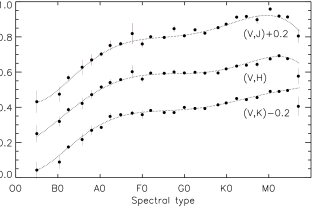
Figure 3: Differential surface brightness for (from top to bottom) the (V, J), (V, H) and (V, Ks), photometric pairs versus spectral type. The (V, J) and (V, Ks) curves have been shifted by $\pm 0.2$ for clarity. The entries were binned, with an interval of 2.5 subspectral type. The dotted lines represent the best fit with polynomials of degree 6. Note that the spectral metric is not smooth (see text).

Figure 4: Computed diameters as a function of measured diameters, for eight stars recently observed with interferometry and not used for the polynomial fit. Stars with increasing diameter, HD numbers: 209458 (G0V), 189733 (K1.5V), 69830 (G8), 185351 (G9III), 190658 (M2.5III), 183589 (K5I), 95687 (M3I), 97671 (M3I), (Johnson et al., 2014; Boffin et al., 2014; Tanner et al., 2015; Boyajian et al., 2015; Arroyo-Torres et al., 2015). The agreement is excellent, with a mean-squared difference between measured and computed diameters expressed in noise units of 0.5. The straight dotted line corresponds to x=y.

6 Conclusion

Our approach to predict stellar angular diameters is based on the modeling of the relationship between angular diameters and photometries. We developed a new methodology that is based on two reddening-free observables: 1) a distance indicator called pseudomagnitude and 2) the differential surface brightness, a handy quasi-experimental observable, that is independent of distance and specific to each star. This, together with our new database of measured angular diameters, allows us to provide estimates of star diameters with statistical errors of $\sim\!1.1\%$, plus possible biases of $\sim\!2\%$. It permits us to upgrade the JSDC catalog of stellar diameters to about $453\,000$ stars, a tenfold improvement in number of stars and diameter precision.

The polynomial method developed in this work may be used with any photometric system, selecting optical bands that best represent the stellar continuum. However, the exercise has severe limits because the DSB is not smooth. The only way to reduce the biases and to go beyond $1\%$ error is to measure its structure for all spectral types and luminosity classes. This emphasises this importance to get precise photometry with biases smaller than $1\%$ and above all the importance of optical interferometry to get precise and numerous angular diameters.

SP Type	$p$	$\sigma_{p}$	SP Type	$p$	$\sigma_{p}$
O5	0.2432	0.0443	F6	0.5810	0.0025
O6	0.2534	0.0337	F7	0.5822	0.0024
O7	0.2670	0.0255	F8	0.5835	0.0023
O8	0.2830	0.0192	F9	0.5850	0.0022
O9	0.3009	0.0147	G0	0.5867	0.0021
B0	0.3201	0.0116	G1	0.5888	0.0020
B1	0.3401	0.0096	G2	0.5912	0.0020
B2	0.3603	0.0085	G3	0.5939	0.0019
B3	0.3805	0.0077	G4	0.5971	0.0019
B4	0.4003	0.0071	G5	0.6006	0.0019
B5	0.4195	0.0067	G6	0.6045	0.0019
B6	0.4378	0.0062	G7	0.6088	0.0019
B7	0.4551	0.0059	G8	0.6134	0.0020
B8	0.4712	0.0055	G9	0.6183	0.0020
B9	0.4862	0.0053	K0	0.6235	0.0021
A0	0.4998	0.0051	K1	0.6289	0.0021
A1	0.5121	0.0050	K2	0.6345	0.0022
A2	0.5231	0.0049	K3	0.6402	0.0023
A3	0.5329	0.0048	K4	0.6460	0.0025
A4	0.5414	0.0047	K5	0.6518	0.0026
A5	0.5488	0.0046	K6	0.6575	0.0028
A6	0.5551	0.0045	K7	0.6632	0.0029
A7	0.5604	0.0043	K8	0.6686	0.0030
A8	0.5648	0.0041	K9	0.6739	0.0031
A9	0.5684	0.0039	M0	0.6790	0.0029
F0	0.5714	0.0037	M1	0.6838	0.0026
F1	0.5738	0.0034	M2	0.6884	0.0023
F2	0.5757	0.0032	M3	0.6928	0.0025
F3	0.5773	0.0030	M4	0.6971	0.0039
F4	0.5786	0.0028	M5	0.7012	0.0065
F5	0.5798	0.0026	M6	0.7054	0.0104

Table 1: Differential surface brightness polynomial values $p$ and associated errors $\sigma_{p}$ for stars measured in the (V, Ks) photometric pair. The angular diameter (mas) and its statistical relative error may be obtained from Eq. 9 and Eq. 10, replacing X by Ks.

Name Ref(s)	Name Ref(s)	Name Ref(s)	Name Ref(s)	Name Ref(s)	Name Ref(s)
GJ411 59	GJ412A 75	GJ649 82	GJ687 75	HD100029 57, 63, 83	HD100920 19
HD1013 83	HD10144 9	HD101501 74	HD102212 43, 57, 63, 83	HD102328 72	HD102647 9, 66
HD102870 74	HD103605 72	HD10380 36, 56	HD10476 77	HD104985 69	HD106574 72
HD106625 9	HD10697 69, 77	HD107383 82	HD10780 70, 74	HD108907 83	HD109358 74, 83
HD112300 63	HD113049 72	HD113226 56, 63, 83	HD113996 83	HD114710 74	HD114961 36, 43
HD115617 82	HD115659 80	HD117176 69	HD117675 83	HD118904 72	HD119149 23
HD11964 69, 77	HD11977 73	HD119850 75	HD120136 69	HD120477 56, 83	HD121130 83
HD121370 57, 63, 67	HD123139 61	HD123934 14, 16, 22	HD12479 14, 37, 50, 54	HD12533 32, 63	HD126660 74
HD127665 83	HD128167 74	HD12929 40, 46, 48, 56, 63	HD129712 83	HD130948 77	HD131156 74
HD131873 40, 63	HD13189 69	HD131977 65	HD132112 36, 43	HD1326 58, 59, 75	HD132813 63
HD133124 83	HD133208 57, 63, 83	HD133774 23	HD135722 56, 63	HD136202 77	HD136726 72, 83
HD137443 72	HD137759 83	HD138265 72	HD139357 72	HD139663 12	HD140538 77
HD140573 57, 63, 83	HD141795 74	HD142804 36	HD142860 74	HD143107 83	HD143761 69, 82
HD144690 50	HD145675 69	HD146051 63, 78	HD146233 74	HD148387 57, 63, 83	HD148478 47, 63
HD149661 75	HD150383 49	HD150680 57, 63	HD150798 78	HD150997 56, 63, 83	HD1522 83
HD152786 78	HD154345 71	HD156283 46, 56, 63	HD157214 77	HD157681 72	HD158633 77
HD159181 63	HD159561 9	HD160290 72	HD161096 83	HD16141 71	HD16160 58, 59, 75
HD161797 63	HD162003 74	HD163770 63	HD163917 83	HD164058 40, 41, 44, 46, 63	HD164259 74
HD167042 72	HD16765 77	HD168151 77	HD16895 74	HD168988 36	HD169022 9
HD170693 72, 83	HD172167 1, 9, 63	HD172816 17, 23, 29, 34, 36, 37, 55	HD17361 56	HD173667 74	HD17506 63
HD175588 51, 63	HD175726 76	HD175775 18	HD175823 72	HD175865 51, 63	HD176124 36
HD176408 72	HD176411 56	HD176437 79, 81	HD176524 83	HD176678 83	HD17709 63
HD177153 76	HD177724 74	HD177756 81	HD177830 69	HD180540 34, 55	HD180610 83
HD180711 40, 57, 63	HD180809 46, 56	HD181276 56, 83	HD181420 76	HD18191 16, 35	HD182572 74
HD183439 46, 63, 83	HD184171 81	HD185144 70, 74	HD185395 74	HD186408 77	HD186427 69, 77
HD186791 56, 63	HD186815 72	HD186882 81	HD187082 23	HD187637 76	HD188512 56
HD190228 69	HD190360 69	HD190406 76	HD19058 44, 51, 63	HD192781 72	HD19373 74
HD193924 1, 9	HD194093 56, 63	HD195564 77	HD195820 72	HD196777 4, 30, 36	HD197345 32, 63
HD19787 56	HD197989 48, 63	HD198149 56	HD199305 75	HD199665 71	HD19994 69
HD200205 72	HD200905 56, 63	HD201092 68	HD202109 63	HD202850 79	HD203504 83
HD204724 63	HD205435 56	HD20630 74	HD206778 57, 63	HD206860 77	HD206952 83
HD207005 12	HD20902 32, 56, 63	HD209100 65	HD209750 56, 63	HD209950 29	HD209952 1, 9
HD210027 76	HD21019 77	HD210418 74	HD210702 71, 82	HD210745 63	HD212496 56, 83
HD213306 53, 56	HD213558 74	HD214868 56, 72	HD214923 81	HD215648 74	HD215665 56, 63
HD216032 43	HD216131 56, 63	HD216386 2, 63	HD216956 1, 9, 66	HD217014 69, 77	HD217906 44, 46, 48, 51, 52, 63, 80
HD218329 83	HD218356 63	HD218396 76	HD219080 79	HD219134 75	HD219576 36
HD219615 83	HD219623 77	HD221115 56	HD221345 71	HD222368 74	HD222603 77
HD224062 19, 37	HD22484 74	HD224935 64	HD23249 67	HD23319 73	HD23596 69
HD24398 81	HD24512 78	HD25025 63	HD25604 56	HD25705 78	HD27256 73
HD285968 82	HD29139 8, 24, 25, 26, 27, 28, 33, 38, 41, 42, 44, 48, 51, 63	HD30959 78	HD31398 63	HD31767 63	HD31964 63
HD32518 72	HD32630 79	HD33564 82	HD3360 79	HD33793 59	HD34085 1, 9
HD34411 74	HD3546 56	HD35468 1, 9, 81	HD3627 48, 57, 63	HD36389 31, 36, 37, 39, 78	HD36395 59, 75
HD3651 69	HD36673 56	HD36848 73	HD3712 32, 46, 48, 56, 63	HD37128 1, 9	HD38529 69
HD38858 77	HD38944 83	HD39983 43, 54	HD40239 51, 63	HD4128 78	HD42995 60
HD432 56	HD44478 6, 7, 10, 11, 21, 35, 41, 44, 51, 63	HD45348 1, 9, 78	HD45410 71	HD4628 75	HD4656 50
HD48329 13, 43, 45, 50, 56, 63	HD48915 1, 9, 62, 63	HD49933 76	HD49968 30	HD5015 74	HD52089 1, 9
HD5395 56	HD5448 79	HD54605 9	HD54719 83	HD56537 74	HD57423 35
HD5820 23	HD58350 9	HD58946 74	HD59686 69	HD60294 72	HD6210 77
HD62345 83	HD66141 83	HD66811 3, 9	HD6860 32, 41, 44, 46, 48, 51, 63	HD69267 56, 63	HD69897 77
HD70272 46	HD7087 56	HD73108 72	HD74442 36	HD76294 57, 83	HD76827 63
HD79211 75	HD7924 82	HD80007 9	HD8019 23	HD80493 46, 57, 63	HD81797 63, 78
HD81937 74	HD82308 83	HD82885 74	HD83618 83	HD84194 83	HD84441 57, 63
HD8512 83	HD85503 83	HD86663 18, 23, 56	HD86728 74	HD87837 13, 15, 21, 29, 56	HD87901 1, 9
HD88230 58, 59, 75	HD89449 76, 79	HD89758 57, 63	HD90839 74	HD91232 43	HD9138 45
HD9408 56	HD95418 74	HD95608 79	HD95735 58, 58, 75, 75	HD96833 57, 63, 83	HD97603 74
HD97633 79	HD9826 69	HD98262 63	HD9927 46, 56	HD99998 5, 20, 56	HR4518 56
HR9045 56

Table 2: List of stars and associated references of angular diameter measurements that have been retained to calibrate the DSB in this work.

(1) Hanbury Brown et al. (1967); (2) Nather et al. (1970); (3) Davis et al. (1970); (4) Dunham et al. (1973); (5) Dunham et al. (1974); (6) White (1974); (7) Ridgway et al. (1974); (8) Currie et al. (1974); (9) Hanbury Brown et al. (1974); (10) Dunham et al. (1975); (11) Nelson (1975); (12) Harwood et al. (1975); (13) de Vegt (1976); (14) Africano et al. (1976); (15) Glass & Morrison (1976); (16) Ridgway et al. (1977); (17) Africano et al. (1977); (18) Vilas & Lasker (1977); (19) Africano et al. (1978); (20) White (1978b); (21) Boehme (1978); (22) White (1978a); (23) Ridgway et al. (1979); (24) White (1979); (25) Beavers & Eitter (1979); (26) Brown et al. (1979); (27) Panek & Leap (1980); (28) Evans et al. (1980); (29) Ridgway et al. (1980a); (30) Beavers et al. (1980); (31) White (1980); (32) Bonneau et al. (1981); (33) Radick & Africano (1981); (34) Evans & Edwards (1981); (35) Beavers et al. (1981); (36) Ridgway et al. (1982a); (37) Beavers et al. (1982); (38) Ridgway et al. (1982b); (39) White et al. (1982); (40) Faucherre et al. (1983); (41) di Benedetto & Conti (1983); (42) White & Kreidl (1984); (43) Schmidtke et al. (1986); (44) di Benedetto & Rabbia (1987); (45) Stecklum (1987); (46) Hutter et al. (1989); (47) Richichi & Lisi (1990); (48) Mozurkewich et al. (1991); (49) Richichi et al. (1992b); (50) Richichi et al. (1992a); (51) Quirrenbach et al. (1993); (52) Dyck et al. (1995); (53) Mourard et al. (1997); (54) Ragland et al. (1997); (55) Richichi et al. (1998); (56) Nordgren et al. (1999); (57) Nordgren et al. (2001); (58) Lane et al. (2001); (59) Ségransan et al. (2003); (60) Richichi & Calamai (2003); (61) Kervella et al. (2003b); (62) Kervella et al. (2003a); (63) Mozurkewich et al. (2003); (64) Fors et al. (2004); (65) Kervella et al. (2004); (66) Di Folco et al. (2004); (67) Thévenin et al. (2005); (68) Kervella et al. (2008); (69) Baines et al. (2008); (70) Boyajian et al. (2008); (71) Baines et al. (2009); (72) Baines et al. (2010); (73) Cusano et al. (2012); (74) Boyajian et al. (2012a); (75) Boyajian et al. (2012b); (76) Boyajian (2014); (77) Boyajian et al. (2013); (78) Cruzalèbes et al. (2013); (79) Maestro et al. (2013); (80) Arroyo-Torres et al. (2014); (81) Challouf et al. (2014); (82) von Braun et al. (2014); (83) Baines et al. (2014)

Appendix A Linear least squares fit

The data consist of a set of $N_{S}$ stars that are characterized by their measured diameter $\theta$ (corrected for limb-darkening) and $N_{B}$ observed magnitudes. Each star provides $N_{B}-1$ linearly independent pseudomagnitude, which combined with the diameter $\theta$, give $N_{B}-1$ correlated measurements (differential surface brightness) per star. Each measurement is fitted as a function of the stellar spectral type number (from 0 to 69 for O$0$ to M$9$) with a polynomial of degree $m$. The problem is then to evaluate $(m+1)\times(N_{B}-1)$ polynomial coefficients, which we do via a simple linear least squares fit, described below.

A.1 Polynomials calculation

We align the $(N_{B}-1)\times N_{S}$ measurements in a vector ${\mathbf{M}}$, and we define the transition matrix ${\mathbf{T}}$ of dimensions $(N_{B}-1).N_{S}\times(m+1).(N_{B}-1)$ as the derivative of ${\mathbf{M}}$ with respect to the unknowns. For simplicity, we assume that the $N_{S}$ stars are distinct, implying no correlations between the measurements of different stars. This allows us to define $N_{S}$ independent covariance matrices $\mathbf{C}_{i},i=0,1,...,N_{S}-1$,of dimension $(N_{B}-1)\times(N_{B}-1)$. Given the photometric pairs that were selected in this work (V, J),(V, H),(V, Ks), the generic expression of the covariance matrix is

$$\mathbf{C}=\frac{\sigma_{\theta}^{2}}{\theta^{2}\ln(10)^{2}}+0.04\times,$$ (11)

$$\left[\begin{array}[]{ccc}\frac{c_{J}^{2}\sigma_{V}^{2}+c_{V}^{2}\sigma_{J}^{2}}{(c_{V}-c_{J})^{2}}&\frac{c_{J}c_{H}\sigma_{V}^{2}}{(c_{V}-c_{J})\times(c_{V}-c_{H})}&\frac{c_{J}c_{Ks}\sigma_{V}^{2}}{(c_{V}-c_{J})\times(c_{V}-c_{Ks})}\\ \frac{c_{J}\,c_{H}\sigma_{V}^{2}}{(c_{V}-c_{J})\times(c_{V}-c_{H})}&\frac{c_{H}^{2}\sigma_{V}^{2}+c_{V}^{2}\sigma_{H}^{2}}{(c_{V}-c_{H})^{2}}&\frac{c_{H}c_{Ks}\sigma_{V}^{2}}{(c_{V}-c_{H})\times(c_{V}-c_{Ks})}\\ \frac{c_{J}c_{Ks}\sigma_{V}^{2}}{(c_{V}-c_{J})\times(c_{V}-c_{Ks})}&\frac{c_{H}c_{Ks}\sigma_{V}^{2}}{(c_{V}-c_{H})\times(c_{V}-c_{Ks})}&\frac{c_{Ks}^{2}\sigma_{V}^{2}+c_{V}^{2}\sigma_{Ks}^{2}}{(c_{V}-c_{Ks})^{2}}\\ \end{array}\right]$$

where $\theta$ is the measured diameter and $\sigma_{\theta}$ its error, $(\sigma_{V},\sigma_{J},\sigma_{H},\sigma_{Ks})$, and $(c_{V},c_{J},c_{H},c_{Ks})$ are the magnitude errors and the interstellar extinction coefficients in the corresponding bands. Next we place the inverse of the covariance matrices $\{\mathbf{C}_{i}^{-1}\}$ along the diagonal of a matrix $\mathbf{D}$ of dimensions $(N_{B}-1).N_{S}\times(N_{B}-1).N_{S}$. The solution for the polynomial coefficients is contained in a vector $\mathbf{A}$ of dimensions $(m+1)\times(N_{B}-1)$, given by

$$\mathbf{A}=\Big{[}^{t}\mathbf{T}\times\mathbf{D}\times\mathbf{T}\Big{]}^{-1}\times^{t}\mathbf{T}\times\mathbf{D}\times\mathbf{V}.$$ (16)

The covariance matrix $\mathbf{C}_{a}$ of the solution $\mathbf{A}$ is

$$\mathbf{C}_{a}=\Big{[}^{t}\mathbf{T}\times\mathbf{D}\times\mathbf{T}\Big{]}^{-1}.$$ (17)

The reconstructed measurement vector writes: $\mathbf{M}_{r}=\mathbf{T}\times\mathbf{A}$, and the reduced $\chi_{p}^{2}$ of the fitting process is

$$\chi_{p}^{2}=\frac{{}^{t}(\mathbf{M}-\mathbf{M}_{r})\times\mathbf{D}\times(\mathbf{M}-\mathbf{M}_{r})}{N_{S}\times(N_{B}-1)}.$$ (18)

A.2 Diameter calculation

For a given star with a spectral type number $n_{s}$ and an associated pseudomagnitude vector $\mathbf{P}$ of dimension $N_{B}-1$, the reconstructed iest $({\it i}=0,...N_{B}-1)$ diameter $\theta_{i}$ is given by

$$\log(\theta_{i})=\sum_{k=0}^{k=m}\mathbf{A}\big{[}k+i\times(m+1)\big{]}\times n_{s}^{k}-0.2\times\mathbf{P}(i).$$ (19)

The covariance matrix $\mathbf{C}_{d}$ between log diameter estimates writes

$$\mathbf{C}_{d}\big{[}\log(\theta_{i}),\log(\theta_{j})\big{]}=0.04\,\mathrm{cov}\big{[}\mathbf{P}(i),\mathbf{P}(j)\big{]}+.$$ (20)

$$\sum_{k=0}^{k=m}\sum_{l=0}^{l=m}\mathbf{C}_{a}\big{[}k+i\times(m+1),l+j\times(m+1)\big{]}\times n_{s}^{k+l}$$

Let us range the $N_{B}-1$ log diameter estimates within a vector ${\mathbf{R}}$. The mean log diameter $\overline{\log(\theta)}$ and the associated error are

$${\overline{\log(\theta)}}=\frac{\sum\mathbf{C}_{d}^{-1}\times\mathbf{R}}{\sum\mathbf{C}_{d}^{-1}}$$ (21)

$$\sigma\big{[}\overline{\log(\theta)}\big{]}=\Big{[}\sum\mathbf{C}_{d}^{-1}\Big{]}^{-0.5},$$ (22)

where $\sum$ stands for the sum of all the matrix elements. The mean diameter $\overline{\theta}$ and its error are computed as follows:

$$\overline{\theta}=10^{\overline{\log(\theta)}}$$ (23)

$$\sigma(\overline{\theta})=\ln(10)\,\sigma\big{[}\overline{\log(\theta)}\big{]}\times\overline{\theta}.$$ (24)

At last, we define the chi-square $\chi^{2}_{\theta}$ associated with the reconstructed log diameter (from the database) by

$$\chi^{2}_{\theta}=\frac{{}^{t}\mathbf{B}\times[\mathbf{C}_{d}+\sigma_{\theta}^{2}]^{-1}\times\mathbf{B}}{N_{B}-1},$$ (25)

where $\mathbf{B}$ is the vector of the difference between the log of the diameter estimates ($\mathbf{R}$) and that of the measured diameter, and $\sigma_{\theta}$ is the error of the measured log diameter. In the case of a catalog of stars with no measured diameter, we can define an internal $\chi_{\theta}^{2}$, replacing the measured diameter and its error with the mean computed diameter and its error.