Resistive sensor and electromagnetic actuator for feedback stabilization of liquid metal walls in fusion reactors

Abstract

Liquid metal walls in fusion reactors will be subject to instabilities, turbulence, induced currents, error fields and temperature gradients that will make them locally bulge, thus entering in contact with the plasma, or deplete, hence exposing the underlying solid substrate. To prevent this, research has begun to actively stabilize static or flowing free-surface liquid metal layers by locally applying forces in feedback with thickness measurements. Here we present resistive sensors of liquid metal thickness and demonstrate $\bm{j}\times\bm{B}$ actuators, to locally control it.

,

Keywords: Liquid metal wall, feedback stabilization, permanent magnet pump

1 Introduction

In a fusion reactor, bare solid walls would be exposed to high fluxes of energetic particles, fusion neutrons and heat [1, 2]. However, they can be protected by a sufficiently thick [3] liquid metal layer [4] to partly attenuate the neutrons and absorb the heat. Neutron attenuation will reduce the need for maintenance and replacement and possibly reduce radioactive waste. In addition, a flowing layer would facilitate heat removal and reduce thermal stress [4, 5]. Additional benefits might include increased survivability of the solid substrate to the heat and particles released during disruptions [4]. Moreover, LMs are very attractive from the point of view of plasma-material interaction [6]. Finally, rotating walls were predicted [8] and experimentally confirmed [9] to stabilize Resistive Wall Modes, giving access to higher values of $\beta$.

However, free-surface liquid metal layers will tend to be uneven [10] as a result of non-uniform force fields, liquid metal instabilities and turbulence. Uneven LM surfaces could enter in contact with the plasma, limit it (in the sense of acting as a limiter), contaminate it, cool it, and possibly disrupt it, or they might expose the underlying solid wall to damage by heat and neutrons. The main motivation for the present work is to prevent these effects by enforcing uniform thickness by feedback control.

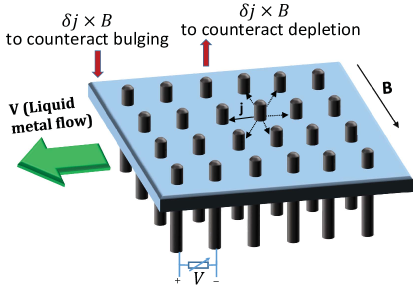
Figure 1: Thickness adjustment by electrodes: stronger (weaker) $j$ is applied where stronger (weaker) $\bm{j}\times\bm{B}$ is needed to counteract liquid metal bulging (depletion).

The key idea is that, in analogy with feedback control of plasma instabilities by arrays of coil sensors and coil actuators [11], liquid metal instabilities can be sensed by ultrasound-, laser- or electrode-based sensors and suppressed by local adjustments of electric current density. Such adjustments would be performed by feedback-controlled arrays of electrodes (Fig.1). Due to the magnetized environment, these would result in local adjustments of the forces that push the liquid against the substrate. Electromagnetic forces can be used alone, serving multiple purposes such as substrate adhesion, flow sustainment and control. Incidentally, a simple balance of Lorentz and gravitational force per unit volume, $\bm{j}\times\bm{B}=\rho g$ shows that levitating Lithium or, equivalently, pushing it against a ”ceiling” requires an amenable 1kA/m² in a 5T reactor. Alternatively, electromagnetic forces can be devoted mostly to control, while adhesion and flow sustainment are delegated to other forces. These include gravity, capillary [11] and centrifugal forces [4] and thermoelectric magnetohydrodynamic forces [12].

The paper is organized as follows. Instabilities and other causes of LM surface unevenness are briefly discussed in Sec.2 and 3. The preparation and characteristics of the working fluid adopted, Galinstan, are described in Sec.4, but the results presented thereafter are easily extended to other liquid metals, more relevant to fusion. Finally, Sec.5 and 6 are devoted to the experimental demonstration of, respectively, resistive sensors of LM thickness and j$\times$B actuators to locally control such thickness, and Sec.7 outlines a strategy for their integration.

2 Timescales and lengthscales of liquid metal instabilities

The two main LM instabilities in a reactor are Rayleigh-Taylor (caused by gravity) and Kelvin-Helmholtz (caused by flow shear).

For the Rayleigh-Taylor instability, consider a LM layer in the ”ceiling” configuration. A perturbation $\delta h=\delta h_{0}\sin kx$ to its thickness $h$ is energetically favorable: the perturbed configuration has lower gravitational potential energy than the unperturbed configuration of uniform thickness $h_{0}$. As a result, the amplitude $\delta h_{0}$ of the perturbation grows with time. Initially, in the limit of small amplitudes, the growth is exponential with growth rate $\gamma=\sqrt{gk\frac{\rho_{2}-\rho_{1}}{\rho_{2}+\rho_{1}}}$ [13], where we have used the fact that the density of the LM, $\rho_{2}$, is much higher than the density of the Scrape Off Layer (SOL) plasma. Hence, perturbations of wavelength $\lambda$= 1-100 cm grow with time-scales of order 13-130 ms. Note that, at wavelengths $\lambda\leq 2\pi\sqrt{\sigma/\rho g}$ (2 cm for Galinstan, 6 cm for Lithium), surface tension $\sigma$ has a stabilizing effect [13]. Short wavelengths are also viscously damped.

In addition, very thin or fast flows are characterized by a large velocity shear and can be susceptible to the Kelvin-Helmholtz instability as a result. In liquid metals the density is approximately uniform, which allows some simplifications. A discrete discontinuity in velocity, of magnitude $\Delta u$ , will cause small perturbations to $h$ to initially grow exponentially, with approximate growth rate $\gamma=k\Delta u/2$ [13, 14]. Hence, in a continuously sheared flow of maximum velocity $u<$1 m/s and $\lambda>$1cm, it is $\gamma\ll$300 s^-1, i.e. the instability grows on timescales much slower than 3 ms.

3 Additional causes of liquid metal non-uniformities

3.1 Non-uniform forces

It was shown in the Introduction that a relatively small current, combined with the 5 T field of a reactor, can easily compete with gravity. However, other currents of comparable magnitude can be present in the liquid metal, induced for example by rotating instabilities in the plasma (Neoclassical Tearing Modes, Resistive Wall Modes and others). These currents are helical and have the same poloidal and toroidal mode number, $m$ and $n$, as the mode in the plasma. The cross- product of the helical j and axisymmetric B will be a spatially modulated j$\times$B force that thickens and thins the LM with periodicity $m$ and $n$. This LM deformation will rotate with the plasma mode, somewhat phase-delayed with respect to it, but it will only grow if the mode in the plasma grows. Due to shielding, at rotation frequencies much higher than the inverse wall time the phase-delay will be maximum, but the LM deformation will be minimum.

Even in the absence of applied or induced $j$, the LM will experience a drag when moving in the magnetic field, due to Lenz’s law. If the field is non-uniform, so will be the drag, and therefore the velocity, causing the LM to pile up or deplete. In the presence of $j$ and non-axisymmetric field $B$ (due to error fields) the force density j$\times$B will also be non-axisymmetric, and cause non-axisymmetries in the LM thickness.

Finally, inhomogeneous LM temperature causes inhomogeneous (1) electrical resistance, (2) viscosity and, to a smaller extent, (3) density. Correspondingly we can expect (1) thermoelectrically driven currents opposite to the temperature gradient, and thus ${\bf j}\times{\bf B}$ forces, (2) flow-shear and possibly convective cells and (3) convective cells as in Bènard instability [13]. All these effects can make the LM flow uneven.

3.2 Turbulence

A liquid metal flowing with sufficiently high Reynolds number in the presence of obstacles and other realistic wall features (such as dents, protrusions, ports, tiles and probes) will be turbulent. Small vortices are actually helpful, as they accelerate transport and speed up heat extraction [15]. However, it will be important to suppress large vortices, which could cause undesired plasma interaction or solid wall exposure. Note that Galinstan has a kinematic viscosity $\nu$ = 3.7$\times$10⁻⁷ m²/s . For a velocity-scale $U$=0.2 m/s and length-scale $L$=0.1 m, this yields a high Reynolds number, $Re$ = 5.4$\times$10⁴. The corresponding flow is definitely turbulent. Comparable values of $Re$ are expected for other LMs in a reactor. This is because the larger $L$ compensates for the higher viscosity of, say, Lithium ( $\nu$ = 1.2$\times$10⁻⁶ m²/s). Also note that, as the liquid metal temperature rises, $\nu$ decreases and hence $Re$ increases, by up to an order of magnitude.

For completeness, the magnetic Reynolds number evaluates $Re_{m}$=0.088, suggesting negligible MHD turbulence in the present experiment. Note however that $Re_{m}$ grows linearly with $L$.

4 Production of Galinstan, corrosion, wetting

For safety and practical reasons, the experiments were carried out with a non-toxic, low-reactive, low melting point (10 ^oC) eutectic alloy of Gallium, Indium and Tin called Galinstan, produced in an electrical furnace. The properties of Galinstan are summarized in Table 1. It is 12 times denser than lithium, approximately as dense as tin, and has acceptable electrical conductivity, similar to lithium. It is corrosive for most metals, with Tungsten being the most corrosion-resistant, but most of our apparatus is made of EPDM rubber, plastic, and 3D-printed PLA plastic, to which Galinstan is not corrosive.

Table 1: Properties of Galinstan and, for comparison, Lithium and Tin

	Galinstan (Ga, In, Sn)	Lithium	Tin
Density	6400 kg/m3	530kg/m3	7000kg/m3
Melting Point	-19oC	181oC	232oC
El. Conductivity	17$\%$ of Copper’s	16$\%$ of Copper’s	14$\%$ of Copper’s
Toxicity	Low	Low	Low
Corrosivity	Very high (corrodes all metals)	Very high	Low

The copper electrodes are among the few exceptions, hence we decided to test their resistance to corrosion by comparing two copper bars of the same dimensions (109.1 $\times$ 34.4 $\times$ 1.1mm). One of them was immersed in Galinstan for 9 weeks, the other was not. Corrosion was surprisingly benign: some corrosion traces and change of color was observed, but neither the lateral dimensions nor the thickness were observed to decrease, within $\pm$0.1 mm, compared to the reference sample.

Galinstan has also a high degree of wetting. This is a desirable property in a reactor, as it prevents the substrate from remaining unwetted and thus unprotected. However, Galinstan tends to wet windows and other surfaces, and obstruct the view of diagnostics. For this reason, we internally coated parts of the setup with Teflon, to counteract wetting.

Galinstan has a very shiny surface, but it oxidizes in contact with air, on a timescale of days. The oxide forms an opaque patina on top of the LM. Such membrane is undesired for several reasons: it alters the dynamics of the fluid underneath, reduces reflectivity to optical probes. Most importantly, the reflected signal would not probe the flow, but the slowly evolving membrane. In addition, the oxide layer has different properties (surface tension, electrical conductivity, heat transfer, outgassing) which might affect the experiment. The increased surface tension, for example, could partly damp the instabilities of interest, and the reduced conductivity could affect thickness measurements. For all these reasons, as well as for consistency with a reactor, where liquid metals will not be exposed to significant amounts of oxygen, experiments were carried out on Galinstan recently cleaned from the oxide layer, by means of a simple wooden tool.

Also note that the experiments were carried out on a timescale of minutes, at most. Timescale separation allowed to ignore corrosion, oxidation and their consequences, such as changes in resistance. In a reactor, LM oxidation will be prevented anyway because it could pose a safety hazard. Corrosion, on the other hand, will need to be accounted for by means of relatively frequent sensor calibrations, every few days or weeks.

The results presented here and in future work for Galinstan on a plastic substrate can be easily adapted to Lithium or other liquid metal on a more fusion-relevant substrate. In fact, from the point of view of the forces required, adhesion and stabilization of Lithium will be 12 times easier than for Galinstan. This is because Lithium is 12 times lighter (see table 1).

5 Demonstration of resistive sensors

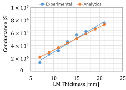
Figure 3: Comparison between the analytical estimates and experimental measurements of liquid metal conductance, as a function of its thickness.

Initially, the system in Fig. 2 was used to resistively measure the thickness of LM in a container, progressively filled with larger and larger amounts of Galinstan. Four-point measurements of conductance were performed in the absence of magnetic field. The measured conductance is plotted in Fig. 3 against the thickness $d$, independently measured by a simple ruler coated with Teflon. As expected, the trend is linear, in agreement with the simple formula $d=L/R\sigma w$ , where $L$ is the distance between the electrodes, $\sigma$ is the electrical conductivity of the liquid metal,$w$ is the width of the container and $R$ is the electrical resistance. The analytical and experimental results are in good agreement, as shown in Fig.3, confirming that the electrical conductance between two electrodes can be used as a proxy for the local LM depth. An intriguing consequence is that imposing uniform conductance is equivalent to imposing uniform thickness. This could be achieved by using the same electrodes as sensors and actuators.

In a more advanced step, the plate electrodes were replaced by wire electrodes, which are less perturbative of the flow. Due to the different shape of the electrodes, a different expression relates the LM thickness $d$ to the resistance $R$ measured between two wire electrodes of radius $r_{0}$, at distance $L$ from each other. To derive this expression, consider the current density $j$ in a point on the axis connecting the two wires, at distance $x$ and $L-x$ from them. This is simply given by $j=\sigma E$, provided $|{\bf v}\times{\bf B}|\ll E$, as it is the case in this experiment, due to the slow flow, relatively high voltages and closely spaced electrodes, resulting in large electric fields $E$. The total electric field is the superposition of the fields generated by the two wires, decaying like the inverse of the distances from said wires. Therefore,

$$j=\frac{I}{2\pi d}\left(\frac{1}{x}+\frac{1}{L-x}\right),$$ (1)

where $I$ is the current flowing from one electrode to the other. The difference of potential $\Delta V$ is the integral of ${\bf E}=\rho{\bf j}$ along any path connecting the two electrodes. Taking the shortest path for simplicity, and substituting the resistance $R=\Delta V/I$, it is concluded that

$$d=\frac{\rho}{\pi R}\ln\frac{L-r_{el}}{r_{el}}$$ (2)

where $\rho$ is the electrical resistivity and $r_{el}$ is the electrical radius of the wire electrode, which is smaller than the actual radius of the electrode, and is defined through calibration tests.

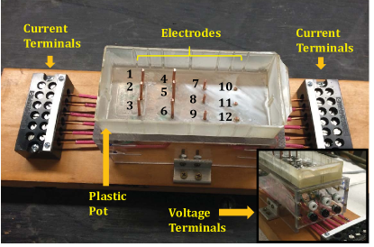
Figure 4: Matrix of 3$\times$4 copper wires (diameter = 2 mm), in three different heights, for resistive measurements of LM thickness.

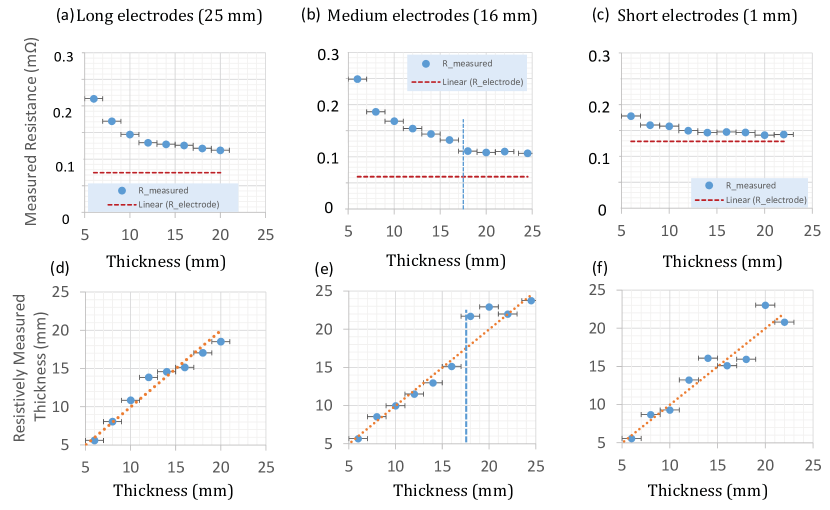
Figure 5: a-c) Resistance measurements between different pairs of electrodes in the setup of Fig.4, as a function of liquid metal thickness. Electrodes considered are respectively 1 and 2 (25 mm tall), 7 and 8 (16 mm tall) and 10 and 11 (1 mm tall). Discontinuity at 16 mm in Fig.b is due to surface tension. d-f) Corresponding resistive measurements of thickness, as a function of the actual thickness.

A matrix of 3$\times$4 copper wire electrodes of 2 mm diameter is shown in Figure 4. The six electrodes on the left are always taller than the LM, i.e. they partly protrude from it; three electrodes in the center are marginal (about as tall as the LM, or slightly shorter) and the three on the right are very short, always immersed in the LM. Each has its own advantages and disadvantages. Electrodes of marginal height, for instance, provide a visual warning about the liquid metal depleting too much or bulging too much, every time the electrode tip protrudes or disappears. In fact, they also provide an electrical warning, via the discontinuity in measured resistance visible in Fig.5b, due to surface tension effects. On the other hand, solid electrodes that protrude permanently or temporarily from the liquid metal would defeat the purpose of protecting solid plasma-facing components from heat and particles, and protecting the plasma from erosion, recycling, etc.

Thin electrodes, 2 mm in diameter and 1 mm in height, do not add any significant friction and turbulence to those caused by tile gaps, welding marks and other small features. The Reynolds number for $L$=1-2 mm is 50-100 smaller than the value, $Re=5.3\times 10^{-4}$, provided above. The “wall-bounded” turbulence caused by these small features is also small compared with “free” turbulence maintained by mean-flow shear in the bulk of the fluid, especially if the fluid is thicker or much thicker. That said, some turbulence is actually beneficial from the point of view of mixing the heat in the LM volume and avoiding excessive surface heating (which reduces the flow-rate required for heat-removal). Also, thin electrodes exhibit a weaker dependence on LM thickness, probably because, as the LM thickness increases, the active size of the electrodes remains unchanged. As a consequence, the height of the current-pattern in the LM increases primarily in between the electrodes, but not much in their vicinity. Thus, the overall effect on the reduction of resistance is not as pronounced as for tall electrodes.

Despite such differences, all resistive measurements of thickness $d$ agreed well with the actual thickness, measured with a simple Teflon-coated ruler, as shown in Figs.5d-f. As expected, $R$ in Figs.5a-c decreased like $1/d$. A vertical offset is also noticeable, which was ascribed to parasitic resistance due to unwanted electrode-coating with metal oxide. Such parasitic resistance is easily quantified in the fitting (calibration) of the said offset. The ultimate result is a very good agreement between the resistively measured thickness and the actual thickness.

As it will be discussed in greater detail in a separate work [16], resistive sensors easily meet the $\sim$10 ms time resolution requirements mentioned in Sec.2. Their response is only expected to be limited by the $L/R$ time of the sensor circuit, sample rate, and multiplexing among several sensors.

6 Demonstration of $\bm{j}\times\bm{B}$ actuator

A setup has been implemented to apply a Lorentz force on the liquid metal and measure the corresponding displacement (Fig. 2). An electromagnet generates a magnetic field of up to 0.4 T in its air-gap. The liquid metal container, of section 15cm x 6cm, is placed in the air-gap of the electromagnet. A current generator applies a DC current (maximum 600A) between the two copper electrodes immersed in the liquid metal container. The current is measured via shunt resistors connected in series with the generator output. The liquid metal depth is measured with a simple Teflon-coated ruler (Fig. 2(c)).

For a DC magnetic field $B_{max}=0.4$T and applied current $I_{max}=200$A, the force was strong enough to visibly push the liquid metal surface downward (Fig. 6). The measured displacement relative to the unperturbed LM level increased with the applied current, as expected (Fig. 7). The displacement should eventually aim asymptotically to the initial unperturbed height $H=2$ cm (quite simply, the level of an initially 2 cm thick LM layer can only be lowered by 2 cm, at most). More data-points are needed to confirm this trend, $h=jBH/(\rho g+jB)$ , expected from a simple force balance. A slightly reduced slope can be noticed at 0-50 A, and might be due to surface tension being non-negligible when the Lorentz force is small, and needing to be included in the force balance.

The response-time of the LM to the actuator depends on the LM inertia and on the available $j$ and $B$, determining the available force. If the sensors, control algorithm and actuators respond within the timescale for the linear instability of interest ($>$10 ms, see Sec.2), the otherwise exponentially growing LM deformation will grow like $t$ or $t^{2}$, on that short timescale, and will rarely exceed $gt^{2}/2$. This suggests that, in general, gravity-defying forces, requiring relatively modest values of $j$ (see Introduction), are sufficient. Finally, the slew-rate for $j$ affects the rate of change of the force. Changes over $\sim$10 ms are amenable and sufficient.

7 Sensor and actuator strategy

The currents applied for the purpose of measuring electrical conductance, proportional to height, can be small. Higher currents are necessary to apply stabilizing or gravity-defying ${\bf j}\times{\bf B}$ forces, but, in principle, the same high ${\bf j}$ could simultaneously sense thickness and serve as actuators.

An alternative strategy can also be envisioned, in which a square-waveform generator alternatively activates a sensor and an actuator circuit (Fig.8). Time-gaps without sensors or without actuators are tolerable, provided they are briefer than the timescale of interest, discussed in Sec.2.

In the sensor circuit (Fig.8a), insulated-gate bipolar transistors (IGBTs) act as switches injecting the currents $I_{s...i,j}$, for example from one boundary of the electrode matrix to the opposite one. Simultaneous voltage and current measurements through each electrode will provide the necessary data to evaluate the LM thickness at every electrode.

If the LM surface is perfectly even, electrical resistivity will be spatially uniform. If not, it will be necessary to use actuators to locally control the LM thickness. A simple criterion for a control system could consist of imposing uniform resistivity.

The anti-parallel arrangement of IGBT switches depicted in Fig.8b provides a bidirectional current path. Adequate compensating current density ${\bf j}_{a}$, calculated at the previous (sensing) stage, will be applied to the proper adjacent electrodes, as to localy exert a ${\bf j}_{a}\times{\bf B}$ force, where needed to even out the LM surface. Similar to the sensor current, the actuator compensating current is pulsating. Therefore ${\bf j}_{a}$ must be defined so that its time-average $<{\bf j}_{a}>$ equals the desired cw current.

8 Summary

Liquid metal (LM) walls in a fusion reactor will be subject to Rayleigh-Taylor and Kelvin-Helmholtz instabilities and, if fast enough, they will become turbulent. For these reasons, and due to induced currents, error fields and temperature gradients, LM walls will tend to be uneven. Work has thus begun to control the thickness of LM layers and prevent them from bulging into the plasma or expose the underlying solid substrate. To that end, here we demonstrated simple sensor and actuator technologies for potential use in future control system. In particular, electrodes were used for measurements of electrical resistance, which were easily interpreted in terms of LM thickness, and and electromagnetic actuator applying j$\times$B forces was used to locally control the film thickness. The next step will consist in interfacing multiple sensors to multiple actuators via a feedback control algorithm.

The present experiments were carried out with Galinstan, but are easily extended to Lithium or other LM. Experiments were conducted in the absence of plasma; future work will be needed in its presence.

References

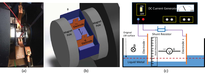
Figure 2: a) Photograph and b) computer rendering (bird’s-eye view) of experimental setup used for resistive measurements of LM thickness by means of plate electrodes. c) Schematic cross-section of setup for demonstration of j$\times$B actuator, allowing LM thickness to decrease between electrodes and increase elsewhere.

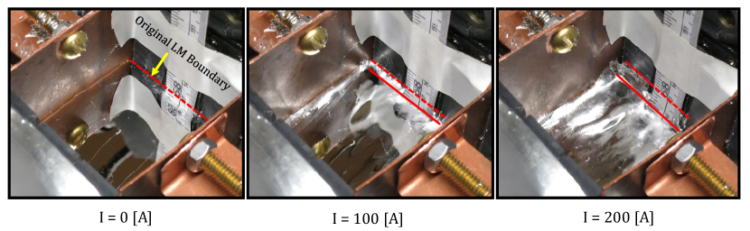
Figure 6: Evidence that the liquid metal level decreases, in the region between electrodes in the experiment of Fig.2c, as a result of increased applied current.

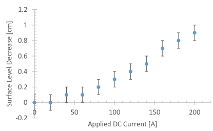
Figure 7: The liquid metal level decreases, in the region between electrodes in the experiment of Fig.2c, as a linear function of the applied current.

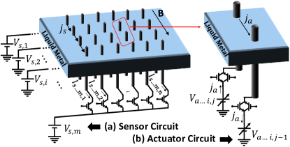
Figure 8: a) Scheme of the Sensor circuit. IGBT switches control when the current is applied to the circuit and b) actuator circuit; anti-parallel IGBT bundle controls a bi-directional current path through each electrode. Subscripts $s$ and $a$ refer respectively to sensors and actuators, subscripts $i$ and $j$ refer to a specific electrode in a matrix of $m\times n$ electrodes.

References

- [1] Cook I 2006 Nat. Mater. 5 77
- [2] Moeslang A et al. 2006 Nat. Mater. 5 679
- [3] Freidberg J P 2007 EURISOL DS, Preliminary report
- [4] Abdou M A et al 2001 Fusion Engineering and Design 54 181-–247
- [5] Abdou M A 1999 Fus. Eng. and Des. 45 145–167
- [6] Majeski R 2015 Plas.-Mat. Interact. Commun. Worksh. (Princeton)
- [7] Majeski R 2016, private communication
- [8] Umansky M V 2001 Phys. Plasmas 8 4427
- [9] Paz-Soldan C et al. 2011 Phys. Rev. Let. 107 245001
- [10] Narula M et al. 2006 Fus. Eng. Des. 81 1543
- [11] Mauel M E et al. 2005 Nucl. Fusion 45 285
- [12] Ruzic D N et al. 2011 Nucl. Fusion 51 102002
- [13] Chandrasekhar S 1981 Hydrodynamic and Hydromagnetic Stability Dover, New York
- [14] Kundu P J and Cohen I M 2004 Flu. Mech. Elsevier
- [15] Kull H J 1991 Phys. Rep. 197
- [16] Mirhoseini S.H.M. and Volpe F.A., arxiv:1606.04008