Learning Local Dependence In Ordered Data

Abstract

In many applications, data come with a natural ordering. This ordering can often induce local dependence among nearby variables. However, in complex data, the width of this dependence may vary, making simple assumptions such as a constant neighborhood size unrealistic. We propose a framework for learning this local dependence based on estimating the inverse of the Cholesky factor of the covariance matrix. Penalized maximum likelihood estimation of this matrix yields a simple regression interpretation for local dependence in which variables are predicted by their neighbors. Our proposed method involves solving a convex, penalized Gaussian likelihood problem with a hierarchical group lasso penalty. The problem decomposes into independent subproblems which can be solved efficiently in parallel using first-order methods. Our method yields a sparse, symmetric, positive definite estimator of the precision matrix, encoding a Gaussian graphical model. We derive theoretical results not found in existing methods attaining this structure. In particular, our conditions for signed support recovery and estimation consistency rates in multiple norms are as mild as those in a regression problem. Empirical results show our method performing favorably compared to existing methods. We apply our method to genomic data to flexibly model linkage disequilibrium. Our method is also applied to improve the performance of discriminant analysis in sound recording classification.

1 Introduction

Estimating large inverse covariance matrices is a fundamental problem in modern multivariate statistics. Consider a random vector $X=\left(X_{1},\ldots,X_{p}\right)^{T}\in{\mathbb{R}}^{p}$ with mean zero and covariance matrix $E(XX^{T})=\Sigma$. Unlike the covariance matrix, which captures marginal correlations among variables in $X$, the inverse covariance matrix $\Omega=\Sigma^{-1}$ (also known as the precision matrix) characterizes conditional correlations and, under a Gaussian model, $\Omega_{jk}=0$ implies that $X_{j}$ and $X_{k}$ are conditionally independent given all other variables. When $p$ is large, it is common to regularize the precision matrix estimator by making it sparse (see, e.g., Pourahmadi, 2013). This paper focuses on the special context in which variables have a natural ordering, such as when data are collected over time or along a genome. In such a context, it is often reasonable to assume that random variables that are far away in the ordering are less dependent than those that are close together. For example, it is known that genetic mutations that occur close together on a chromosome are more likely to be coinherited than mutations that are located far apart. We propose a method for estimating the precision matrix based on this assumption while also allowing each random variable to have its own notion of closeness.

In general settings where variables do not necessarily have a known ordering, two main types of convex methods with strong theoretical results have been developed for introducing sparsity in $\Omega$. The first approach, known as the graphical lasso (Yuan and Lin, 2007; Banerjee et al., 2008; Friedman et al., 2008; Rothman et al., 2008), performs penalized maximum likelihood, solving $\min_{\Omega\succ 0,\Omega=\Omega^{T}}\mathcal{L}\left(\Omega\right)+\lambda P\left(\Omega\right)$, where $\mathcal{L}(\Omega)=-\log\det\Omega+n^{-1}\sum_{i=1}^{n}x_{i}^{T}\Omega x_{i}$ is, up to constants, the negative log-likelihood of a sample of $n$ independent Gaussian random vectors and $P(\Omega)$ is the (vector) $\ell_{1}$-norm of $\Omega$. Zhang and Zou (2014) introduce a new convex loss function called the D-trace loss and propose a positive definite precision matrix estimator by minimizing an $\ell_{1}$-penalized version of this loss. The second approach is through penalized pseudo-likelihood, the most well-known of which is called neighborhood selection (Meinshausen and Bühlmann, 2006). Estimators in this category are usually solved by a column-by-column approach and thus are more amenable to theoretical analysis (Yuan, 2010; Cai et al., 2011; Liu and Luo, 2012; Liu and Wang, 2012; Sun and Zhang, 2013; Khare et al., 2014). However they are not guaranteed to be positive definite and do not exploit the symmetry of $\Omega$. Peng et al. (2009) propose a partial correlation matrix estimator that develops a symmetric version of neighborhood selection; however, positive definiteness is still not guaranteed.

In the context of variables with a natural ordering, by contrast, almost no work uses convex optimization to flexibly estimate $\Omega$ while exploiting the ordering structure. Sparsity is usually induced via the Cholesky decomposition of $\Sigma$, which leads to a natural interpretation of sparsity. Consider the Cholesky decomposition $\Sigma=QQ^{T}$, which implies $\Omega=L^{T}L$ for $L=Q^{-1}$ for lower triangular matrices $Q$ and $L$ with positive diagonals. The assumption that $X\sim N\left(0,\Sigma\right)$ is then equivalent to a set of linear models in terms of rows of $L$, i.e., $L_{11}X_{1}=\varepsilon_{1}$ and

$$L_{rr}X_{r}=-\sum_{k=1}^{r-1}L_{rk}X_{k}+\varepsilon_{r}\quad r=2,\ldots,p,$$ (1)

where $\varepsilon\sim N\left(0,I_{p}\right)$. Thus, $L_{rk}=0$ (for $k<r$) can be interpreted as meaning that in predicting $X_{r}$ from the previous random variables, one does not need to know $X_{k}$. This observation has motivated previous work, including Pourahmadi (1999); Wu and Pourahmadi (2003); Huang et al. (2006); Shojaie and Michailidis (2010); Khare et al. (2016). While these methods assume sparsity in $L$, they do not require local dependence because each variable is allowed to be dependent on predecessors that are distant from it (compare the upper left to the upper right panel of Figure 10).

The assumption of “local dependence” can be expressed as saying that each variable $X_{r}$ can be best explained by exactly its $K_{r}$ closest predecessors:

$$L_{rr}X_{r}=-\sum_{k=r-K_{r}}^{r-1}L_{rk}X_{k}+\varepsilon_{r},\quad\text{for}\quad L_{rk}\neq 0,\quad r-K_{r}\leq k\leq r-1,\quad r=2,\ldots,p.$$ (2)

Note that this does not describe all patterns of a variable depending on its nearby variables. For example, $X_{r}$ can be dependent on $X_{r-2}$ but not on $X_{r-1}$. In this case, the dependence is still local, but would not be captured by (2). We focus on the restricted class (2) since it greatly simplifies the interpretation of the learned dependence structure by capturing the extent of this dependence in a single number $K_{r}$, the neighborhood size.

Another desirable property of model (2) is that it admits a simple connection between the sparsity pattern of $L$ and the sparsity pattern of the precision matrix $\Omega$ in the Gaussian graphical model. In particular, straightforward algebra shows that for $j<k$,

$$L_{kj}=\dots=L_{pj}=0\implies\Omega_{jk}=0.$$ (3)

Statistically, this says that if none of the variables $X_{k},\dots,X_{p}$ depends on $X_{j}$ in the sense of (1), then $X_{j}$ and $X_{k}$ are conditionally independent given all other variables.

Bickel and Levina (2008) study theoretical properties in the case that all bandwidths, $K_{r}$, are equal, in which case model (2) is a $K_{r}$-ordered antedependence model (Zimmerman and Nunez-Anton, 2009). A banded estimate of $L$ then induces a banded estimate of $\Omega$. The nested lasso approach of Levina et al. (2008) provides for “adaptive banding”, allowing $K_{r}$ to vary with $r$ (which corresponds to variable-order antedependence models in Zimmerman and Nunez-Anton, 2009); however, the nested lasso is non-convex, meaning that the proposed algorithm does not necessarily minimize the stated objective and theoretical properties of this estimator have not been established.

In this paper, we propose a penalized likelihood approach that provides the flexibility of the nested lasso but is formulated as a convex optimization problem, which allows us to prove strong theoretical properties and to provide an efficient, scalable algorithm for computing the estimator. The theoretical development of our method allows us to make clear comparisons with known results for the graphical lasso (Rothman et al., 2008; Ravikumar et al., 2011) in the non-ordered case. Both methods are convex penalized likelihood approaches, so this comparison highlights the similarities and differences in the ordered and non-ordered problems.

There are two key choices we make that lead to a convex formulation. First, we express the optimization problem in terms of the Cholesky factor $L$. The nested lasso and other methods (starting with Pourahmadi 1999) use the modified Cholesky decomposition, $\Omega=T^{T}D^{-1}T$, where $T$ is a lower-triangular matrix with ones on its diagonal and $D$ is a diagonal matrix with positive entries. While $\mathcal{L}(\Omega)$ is convex in $\Omega$, the negative log-likelihood $\mathcal{L}(T^{T}D^{-1}T)$ is not jointly convex in $T$ and $D$. By contrast,

$$\mathcal{L}\left(L^{T}L\right) =-\log\det\left(L^{T}L\right)+\frac{1}{n}\sum_{i=1}^{n}{x}_{i}^{T}L^{T}L{x}_{i}=-2\sum_{r=1}^{p}\log L_{rr}+\frac{1}{n}\sum_{i=1}^{n}\left\lVert L{x}_{i}\right\rVert_{2}^{2}$$ (4)

is convex in $L$. This parametrization is considered in Aragam and Zhou (2015), Khare et al. (2014), and Khare et al. (2016). Maximum likelihood estimation of $L$ preserves the regression interpretation by noting that

$$\mathcal{L}\left(L^{T}L\right)=-2\sum_{r=1}^{p}\log L_{rr}+\frac{1}{n}\sum_{r=1}^{p}\sum_{i=1}^{n}L_{rr}^{2}\left(x_{ir}+\sum_{k=1}^{r-1}L_{rk}x_{ik}/L_{rr}\right)^{2}.$$

This connection has motivated previous work with the modified Cholesky decomposition, in which $T_{rk}=-L_{rk}/L_{rr}$ are the coefficients of a linear model in which $X_{r}$ is regressed on its predecessors, and $D_{rr}=L_{rr}^{-2}$ corresponds to the error variance. The second key choice is our use of a hierarchical group lasso in place of the nested lasso’s nonconvex penalty.

We introduce here some notation used throughout the paper. For two sequences of constants $a(n)$ and $b(n)$, the notation $a(n)=o\left(b(n)\right)$ means that for every $\varepsilon>0$, there exists a constant $N>0$ such that $|a(n)/b(n)|\leq\varepsilon$ for all $n\geq N$. And the notation $a(n)=\mathcal{O}\left(b(n)\right)$ means that there exists a constant $N>0$ and a constant $M>0$ such that $|a(n)/b(n)|\leq M$ for all $n\geq N$. For a sequence of random variables $A(n)$, the notation $A(n)=\mathcal{O}_{P}\left(b(n)\right)$ means that for every $\varepsilon>0$, there exists a constant $M>0$ such that $\mathrm{P}\left(|A(n)/b(n)|>M\right)\leq\varepsilon$ for all $n$.

For a vector $v=\left(v_{1},\ldots,v_{p}\right)\in\mathbb{R}^{p}$, we define $\left\lVert v\right\rVert_{1}=\sum_{j=1}^{p}|v_{j}|$, $\left\lVert v\right\rVert_{2}=(\sum_{j=1}^{p}v_{j}^{2})^{1/2}$ and $\left\lVert v\right\rVert_{\infty}=\max_{j}|v_{j}|$. For a matrix $M\in\mathbb{R}^{n\times p}$, we define the element-wise norms by two vertical bars. Specifically, $\left\lVert M\right\rVert_{\infty}=\max_{jk}|M_{jk}|$ and Frobenius norm $\left\lVert M\right\rVert_{F}=(\sum_{j,k}M_{jk}^{2})^{1/2}$. For $q\geq 1$, we define the matrix-induced (operator) $q$-norm by three vertical bars: ${\left|\kern-1.07639pt\left|\kern-1.07639pt\left|M\right|\kern-1.07639pt\right|\kern-1.07639pt\right|}_{q}=\max_{\left\lVert v\right\rVert_{q}=1}\left\lVert Mv\right\rVert_{q}$. Important special cases include ${\left|\kern-1.07639pt\left|\kern-1.07639pt\left|M\right|\kern-1.07639pt\right|\kern-1.07639pt\right|}_{2}$, also known as the spectral norm, which is the largest singular value of $M$, as well as ${\left|\kern-1.07639pt\left|\kern-1.07639pt\left|M\right|\kern-1.07639pt\right|\kern-1.07639pt\right|}_{1}=\max_{k}\sum_{j=1}^{p}|M_{jk}|$ and ${\left|\kern-1.07639pt\left|\kern-1.07639pt\left|M\right|\kern-1.07639pt\right|\kern-1.07639pt\right|}_{\infty}=\max_{j}\sum_{k=1}^{p}|M_{jk}|$. Note that ${\left|\kern-1.07639pt\left|\kern-1.07639pt\left|M\right|\kern-1.07639pt\right|\kern-1.07639pt\right|}_{1}={\left|\kern-1.07639pt\left|\kern-1.07639pt\left|M\right|\kern-1.07639pt\right|\kern-1.07639pt\right|}_{\infty}$ when $M$ is symmetric.

Given a $p$-vector $v$, a $p\times p$ matrix $M$, and an index set $T$, let $v_{T}=(v_{i})_{i\in T}$ be the $|T|$-subvector and $M_{T}$ the $p\times|T|$ submatrix with columns selected from $T$. Given a second index set $T^{\prime}$, let $M_{TT^{\prime}}$ be the $|T|\times|T^{\prime}|$ submatrix with rows and columns of $M$ indexed by $T$ and $T^{\prime}$, respectively. Specifically, we use $L_{r\cdot}$ to denote the $r$-th row of $L$.

2 Estimator

For a given tuning parameter $\lambda\geq 0$, we define our estimator $\hat{L}$ to be a minimizer of the following penalized negative Gaussian log-likelihood

$$\hat{L}\in\operatorname*{arg\,min}_{\begin{subarray}{c}L:L_{rr}>0\\ L_{rk}=0\text{ for }r<k\end{subarray}}\left\{-2\sum_{r=1}^{p}\log L_{rr}+\frac{1}{n}\sum_{i=1}^{n}\left\lVert L{x}_{i}\right\rVert_{2}^{2}+\lambda\sum_{r=2}^{p}P_{r}\left(L_{r\cdot}\right)\right\}.$$ (5)

The penalty $P_{r}$, which is applied to the $r$-th row, is defined by

$$P_{r}\left(L_{r\cdot}\right)=\sum_{\ell=1}^{r-1}\left\lVert W^{(\ell)}\ast L_{g_{r,\ell}}\right\rVert_{2}=\sum_{\ell=1}^{r-1}\left(\sum_{m=1}^{\ell}w_{\ell m}^{2}L_{rm}^{2}\right)^{1/2},$$ (6)

where $W^{(\ell)}=(w_{\ell 1},\ldots,w_{\ell\ell})\in\mathbb{R}^{\ell}$ is a vector of weights, $\ast$ denotes element-wise multiplication, and $L_{g_{r,\ell}}$ denotes the vector of elements of $L$ from the group $g_{r,\ell}$, which corresponds to the first $\ell$ elements in the $r$-th row (for $1\leq\ell\leq r-1$):

$$g_{r,\ell}=\left\{(r,\ell^{\prime}):\ell^{\prime}\leq\ell\right\}.$$

Since $g_{r,1}\subset g_{r,2}\subset\cdots\subset g_{r,r-1}$, each row $r$ of $L$ is penalized with a sum of $r-1$ nested, weighted $\ell_{2}$-norm penalties. This is a hierarchical group lasso penalty (Yuan and Lin, 2007; Zhao et al., 2009; Jenatton et al., 2011; Yan and Bien, 2015) with group structure conveyed in Figure 1.

With $w_{\ell m}>0$, this nested structure always puts more penalty on those elements that are further away from the diagonal. Since the group lasso has the effect of setting to zero a subset of groups, it is apparent that this choice of groups ensures that whenever the elements in $g_{r,\ell}$ are set to zero, elements in $g_{r,\ell^{\prime}}$ are also set to zero for all $\ell^{\prime}\leq\ell$. In other words, for each row of $\hat{L}$, the non-zeros are those elements within some (row-specific) distance of the diagonal. This is in contrast to the $\ell_{1}$-penalty as used in Khare et al. (2016), which produces sparsity patterns with no particular structure (compare the top-left and top-right panels of Figure 10).

The choice of weights, $w_{\ell m}$, affects both the empirical and theoretical performance of the estimator. We focus primarily on a quadratically decaying set of weights,

$$w_{\ell m}=\frac{1}{\left(\ell-m+1\right)^{2}},$$ (7)

but also consider the unweighted case (in which $w_{\ell m}=1$). The decay counteracts the fact that the elements of $L$ appear in differing numbers of groups (for example $L_{r1}$ appears in $r-1$ groups whereas $L_{r,r-1}$ appears in just one group). In a related problem, Bien et al. (2016) choose weights that decay more slowly with $\ell-m$ than (7). Our choice makes the enforcement of hierarchy weaker so that our penalty behaves more closely to the lasso penalty (Tibshirani, 1996). The choice of weight sequence in (7) is more amenable to theoretical analysis; however, in practice the unweighted case is more efficiently implemented and works well empirically.

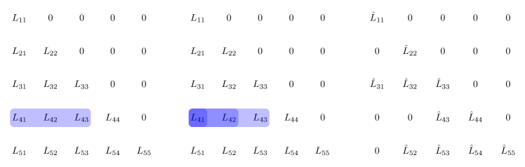
Figure 1: There are $p\choose 2$ groups used in the penalty, with each row $r$ having $r-1$ nested groups $g_{r,1}\subset g_{r,2}\subset\cdots\subset g_{r,r-1}$. Left: the group $g_{4,3}$. Middle: the nested group structure $g_{4,1}\subset g_{4,2}\subset g_{4,3}$. Right: A possible sparsity pattern in $\hat{L}$, where elements in $g_{2,1},g_{4,2}$ (and thus $g_{4,1}$) and $g_{5,1}$ are set to zero.

Problem (5) is convex in $L$. While $-\log\det(\cdot)$ is strictly convex, $-\sum_{r}\log(L_{rr})$ is not strictly convex in $L$. Thus, the $\operatorname*{arg\,min}$ in (5) may not be unique. In Section 4, we provide sufficient conditions to ensure uniqueness with high probability.

In Appendix A, we show that (5) decouples into $p$ independent subproblems, each of which estimates one row of $L$. More specifically, let $\mathbf{X}\in\mathbb{R}^{n\times p}$ be a sample matrix with independent rows $x_{i}\sim N(0,\Sigma)$, $\hat{L}_{11}=n^{1/2}(\mathbf{X}_{1}^{T}\mathbf{X}_{1})^{-1/2}$ and for $r=2,\ldots,p$,

$$\hat{L}_{r,1:r}=\operatorname*{arg\,min}_{\beta\in\mathbb{R}^{r}:\beta_{r}>0}\left\{-2\log\beta_{r}+\frac{1}{n}\left\lVert\mathbf{X}_{1:r}\beta\right\rVert_{2}^{2}+\lambda\sum_{\ell=1}^{r-1}\left(\sum_{m=1}^{\ell}w_{\ell m}^{2}\beta_{m}^{2}\right)^{1/2}\right\}.$$ (8)

This observation means that the computation can be easily parallelized, which potentially can achieve a linear speed up with the number of CPU cores. Theoretically, to analyze the properties of $\hat{L}$ it is easier to start by studying an estimator of each row, i.e., a solution to (8). We will see in Section 4 that problem (8) has connections to a penalized regression problem, meaning that both the assumptions and results we can derive are better than if we were working with a penalty based on $\Omega$.

In light of the regression interpretation of (1), $\hat{L}$ provides an interpretable notion of local dependence; however, we can of course also use our estimate of $L$ to estimate $\Omega$: $\hat{\Omega}=\hat{L}^{T}\hat{L}$. By construction, this estimator is both symmetric and positive definite. Unlike a lasso penalty, which would induce unstructured sparsity in the estimate of $L$ and thus would not be guaranteed to produce a sparse estimate of $\Omega$, the adaptively banded structure in our estimator of $L$ can yield a generally banded $\hat{\Omega}$ with sparsity pattern determined by (3) (See the top-left and bottom-left panels in Figure 10 for an example).

3 Computation

As observed above, we can compute $\hat{L}$ by solving (in parallel across $r$) problem (8). Consider an alternating direction method of multipliers (ADMM) approach that solves the equivalent problem

$$\min_{\beta,\gamma\in\mathbb{R}^{r}:\beta_{r}>0}\left\{-2\log\beta_{r}+\frac{1}{n}\left\lVert\mathbf{X}_{1:r}\beta\right\rVert_{2}^{2}+\lambda\sum_{\ell=1}^{r-1}\left({\sum_{m=1}^{\ell}w_{\ell m}^{2}\gamma_{m}^{2}}\right)^{1/2}\mathrm{\quad s.t.\quad}\beta=\gamma\right\}.$$

Algorithm 1 presents the ADMM algorithm, which repeatedly minimizes this problem’s augmented Lagrangian over $\beta$, then over $\gamma$, and then updates the dual variable $u\in\mathbb{R}^{r}$.

Algorithm 1 ADMM algorithm to solve (8)

1:$\beta^{(0)}$, $\gamma^{(0)}$, $u^{(0)}$, $\rho>0$, $t=1$.

2:repeat

3:     

$$\beta^{(t)} \leftarrow\operatorname*{arg\,min}_{\beta\in\mathbb{R}^{r}:\beta_{r}>0}\left\{-2\log\beta_{r}+\frac{1}{n}\left\lVert\mathbf{X}_{1:r}\beta\right\rVert_{2}^{2}+\left(\beta-\gamma^{(t-1)}\right)^{T}u^{(t-1)}+\frac{\rho}{2}\left\lVert\beta-\gamma^{(t-1)}\right\rVert_{2}^{2}\right\}$$ (9)

4:     

$$\gamma^{(t)} \leftarrow\operatorname*{arg\,min}_{\gamma\in\mathbb{R}^{r}}\left\{\frac{\rho}{2}\left\lVert\gamma-\beta^{(t)}-\rho^{-1}u^{(t-1)}\right\rVert_{2}^{2}+\lambda\sum_{\ell=1}^{r-1}\left(\sum_{m=1}^{\ell}w_{\ell m}^{2}\gamma_{m}^{2}\right)^{1/2}\right\}$$ (10)

5:     $u^{(t)}\leftarrow u^{(t-1)}+\rho\left(\beta^{(t)}-\gamma^{(t)}\right)$ 

6:     $t\leftarrow t+1$ 

7:until convergence

8:return $\gamma^{(t)}$

The main computational effort in the algorithm is in solving (9) and (10). Note that (9) has a smooth objective function. Straightforward calculus gives the closed-form solution (see Appendix B for detailed derivation),

$$\beta^{(t+1)}_{r}=\frac{-B-\sqrt{B^{2}-8A}}{2A}>0$$

$$\beta^{(t+1)}_{-r}=-\left(2S^{(r)}_{-r,-r}+\rho I\right)^{-1}\left(2S^{(r)}_{-r,r}\beta^{(t+1)}_{r}+u^{(t)}_{-r}-\rho\gamma^{(t)}_{-r}\right),$$

where

$$S^{(r)}=\frac{1}{n}\mathbf{X}_{1:r}^{T}\mathbf{X}_{1:r}$$

$$A=4S^{(r)}_{r,-r}\left(2S^{(r)}_{-r,-r}+\rho I\right)^{-1}S^{(r)}_{-r,r}-2S^{(r)}_{r,r}-\rho<0$$

$$B=2S^{(r)}_{r,-r}\left(2S^{(r)}_{-r,-r}+\rho I\right)^{-1}\left(u^{(t)}_{-r}-\rho\gamma^{(t)}_{-r}\right)-u^{(t)}_{r}+\rho\gamma^{(t)}_{r}.$$

The closed-form update above involves matrix inversion. With $\rho>0$, the matrix $2S^{(r)}_{-r,-r}+\rho I$ is invertible even when $r>n$. Since determining a good choice for the ADMM parameter $\rho$ is in general difficult, we adapt the dynamic $\rho$ updating scheme described in Section 3.4.1 of Boyd et al. (2011).

Solving (10) requires evaluating the proximal operator of the hierarchical group lasso with general weights. We adopt the strategy developed in Bien et al. (2016) (based on a result of Jenatton et al. 2011), which solves the dual problem of (10) by performing Newton’s method on at most $r-1$ univariate functions. The detailed implementation is given in Algorithm 3 in Appendix C. Each application of Newton’s method corresponds to performing an elliptical projection, which is a step of blockwise coordinate ascent on the dual of (10) (see Appendix D for details). Finally we observe in Algorithm 2 that for the unweighted case ($w_{\ell m}=1$), solving (10) is remarkably efficient.

Algorithm 2 Algorithm for solving (10) for unweighted estimator

1:$\beta^{(t)},u^{(t-1)}\in\mathbb{R}^{r}$, $\lambda,\rho>0$.

2:Initialize $\gamma^{(t)}=\beta^{(t)}+u^{(t-1)}/\rho$ and $\tau=\lambda/\rho$ 

3:for $\ell=1,\ldots,r-1$ do

$$\left(\gamma^{(t)}\right)_{1:\ell}\leftarrow\left(1-\frac{\tau}{\left\lVert\left(\gamma^{(t)}\right)_{1:\ell}\right\rVert_{2}}\right)_{+}\left(\gamma^{(t)}\right)_{1:\ell}$$

4:return $\gamma^{(t)}$.

The R package varband provides C++ implementations of Algorithms 1 and 2.

4 Statistical Properties

In this section we study the statistical properties of our estimator. In what follows, we consider a lower triangular matrix $L$ having row-specific bandwidths, $K_{r}$. The first $J_{r}=r-1-K_{r}$ elements of row $r$ are zero, and the band of non-zero off-diagonals (of size $K_{r}$) is denoted $\mathcal{I}_{r}=\left\{J_{r}+1,\dots,r-1\right\}$. We also denote $\mathcal{I}_{r}^{c}=\left\{1,2,\dots,r\right\}\setminus\mathcal{I}_{r}$. See Figure 2 for a graphical example of $K_{5},J_{5},\mathcal{I}_{4}$, and $\mathcal{I}_{4}^{c}$.

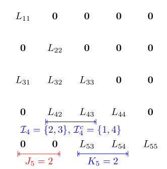
Figure 2: Schematic showing $J_{r},K_{r},\mathcal{I}_{r}$, and $\mathcal{I}_{r}^{c}$.

Our theoretical analysis is built on the following assumptions:

1. Gaussian assumption: The sample matrix $\mathbf{X}\in\mathbb{R}^{n\times p}$ has $n$ independent rows with each row $x_{i}$ drawn from $N(\mathbf{0},\Sigma)$.

2. Sparsity assumption: The true Cholesky factor $L\in\mathbb{R}^{p\times p}$ is the lower triangular matrix with positive diagonal elements such that the precision matrix $\Omega=\Sigma^{-1}=L^{T}L$. The matrix $L$ has row-specific bandwidths $K_{r}$ such that $L_{rj}=0$ for $0<j<r-K_{r}$.

3. Irrepresentable condition: There exists some $\alpha\in(0,1]$ such that

   $$\max_{2\leq r\leq p}\max_{\ell\in\mathcal{I}^{c}_{r}}\left\lVert\Sigma_{\ell\mathcal{I}_{r}}\left(\Sigma_{\mathcal{I}_{r}\mathcal{I}_{r}}\right)^{-1}\right\rVert_{1}\leq\frac{6}{\pi^{2}}\left(1-\alpha\right)$$

4. Bounded singular values: There exists a constant $\kappa$ such that

   $$0<\kappa^{-1}\leq\sigma_{\min}\left(L\right)\leq\sigma_{\max}\left(L\right)\leq\kappa$$

When $\max_{r}K_{r}<n$, the Gaussianity assumption A1 implies that $\mathbf{X}_{\mathcal{I}_{r}}$ has full column rank for all $r$ with probability one. Our analysis applies to the general high-dimensional scaling scheme where $K_{r}=K_{r}(n)$ and $p=p(n)$ can grow with $n$.

For $r=2,\ldots,p$ and $\ell\in{\mathcal{I}}_{r}^{c}=\left\{1,\ldots,J_{r},r\right\}$, let

$$\theta^{(\ell)}_{r}:=\mathrm{Var}\left(X_{\ell}|X_{\mathcal{I}_{r}}\right)\quad\text{and}\quad\theta_{r}:=\max_{\ell\in\mathcal{I}_{r}^{c}}\theta^{(\ell)}_{r}.$$

By Assumption A1, $\theta_{r}^{(\ell)}=\Sigma_{\ell\ell}-\Sigma_{\ell\mathcal{I}_{r}}\left(\Sigma_{\mathcal{I}_{r}\mathcal{I}_{r}}\right)^{-1}\Sigma_{\mathcal{I}_{r}\ell}$ represents the noise variance when regressing $X_{\ell}$ on $X_{\mathcal{I}_{r}}$, i.e., for $\ell=1,\ldots,J_{r},r$,

$$X_{\ell}=\Sigma_{\ell\mathcal{I}_{r}}(\Sigma_{\mathcal{I}_{r}\mathcal{I}_{r}})^{-1}X_{\mathcal{I}_{r}}^{T}+E_{\ell}\qquad\text{with}\qquad E_{\ell}\sim N\left(0,\theta_{r}^{(\ell)}\right).$$ (11)

In words, $\theta_{r}^{(\ell)}$ measures the degree to which $X_{\ell}$ cannot be explained by the variables in the support and $\theta_{r}$ is the maximum such value over all $\ell$ outside of the support $\mathcal{I}_{r}$ in the $r$-th row. Intuitively, the difficulty of the estimation problem increases with $\theta_{r}$. Note that for $r=1,\ldots,p$, (1) implies $\theta^{(r)}_{r}=1/L_{rr}^{2}$.

Assumption A3 (along with the $\beta_{\min}$ condition) is essentially a necessary and sufficient condition for support recovery of lasso-type methods (see, e.g., Zhao and Yu, 2006; Meinshausen and Bühlmann, 2006; Wainwright, 2009; Van de Geer and Bühlmann, 2009; Ravikumar et al., 2011). The constant $\alpha\in(0,1]$ is usually referred to as the irrepresentable (incoherence) constant (Wainwright, 2009). Intuitively, the irrepresentable condition requires low correlations between signal and noise predictors, and thus a value of $\alpha$ that is close to 1 implies that recovering the support is easier to achieve. The constant $6\pi^{-2}$ is determined by the choice of weight (7) and can be eliminated by absorbing its reciprocal into the definition of the weights $w_{\ell m}$. Doing so, one finds that our irrepresentable condition is essentially the same as the one found in the regression setting (Wainwright, 2009) despite the fact that our goal is estimating a precision matrix.

Assumption A4 is a bounded singular value condition. Recalling that $\Omega=L^{T}L$,

$$0<\kappa^{-2}\leq\sigma_{\min}\left(\Sigma\right)\leq\sigma_{\max}\left(\Sigma\right)\leq\kappa^{2},$$ (12)

which is equivalent to the commonly used bounded eigenvalue condition in other literatures.

4.1 Row-Specific Results

We start by analyzing support recovery properties of our estimator for each row, i.e., the solution to the subproblem (8). For $r>n$, the Hessian of the negative log-likelihood is not positive definite, meaning that the objective function may not be strictly convex in $\beta$ and the solution not necessarily unique. Intuitively, if the tuning parameter $\lambda$ is large, the resulting row estimate $\hat{L}_{r\cdot}$ is sparse and thus includes most variation in a small subset of the $r$ variables. More specifically, for large $\lambda$, $\hat{\mathcal{I}}_{r}\subseteq\mathcal{I}_{r}$ and thus by Assumption A1, $\mathbf{X}_{\hat{\mathcal{I}}_{r}}$ has full rank, which implies that $\hat{L}_{r\cdot}$ is unique. The series of technical lemmas in Appendix E precisely characterizes the solution.

The first part of the theorem below shows that with an appropriately chosen tuning parameter $\lambda$ the solution to (8) is sparse enough to be unique and that we will not over-estimate the true bandwidth. Knowing that the support of the unique row estimator $\hat{L}_{r\cdot}$ is contained in the true support reduces the dimension of the parameter space, and thus leads to a reasonable error bound. Of course, if our goal were simply to establish the uniqueness of $\hat{L}_{r\cdot}$ and that $\hat{K}_{r}\leq K_{r}$, we could trivially take $\lambda=\infty$ (resulting in $\hat{K}_{r}=0$). The latter part of the theorem thus goes on to provide a choice of $\lambda$ that is sufficiently small to guarantee that $\hat{K}_{r}=K_{r}$ (and, furthermore, that the signs of all non-zeros are correctly recovered).

Theorem 1.

Consider the family of tuning parameters

$$\lambda=\frac{8}{\alpha}\sqrt{\frac{\theta_{r}\log r}{n}}$$ (13)

and weights given by (7). Under Assumptions A1–A4, if the tuple $\left(n,J_{r},K_{r}\right)$ satisfies

$$n>\alpha^{-2}\left(3\pi^{2}K_{r}+8\right)\theta_{r}\kappa^{2}\log J_{r},$$ (14)

then with probability greater than $1-c_{1}\exp\left\{-c_{2}\min(K_{r},\log J_{r})\right\}-7\exp\left(-c_{3}n\right)$ for some constants $c_{1},c_{2},c_{3}$ independent of $n$ and $J_{r}$, the following properties hold:

1. The row problem (8) has a unique solution $\hat{L}_{r\cdot}$ and $\hat{K}_{r}\leq K_{r}$.

2. The estimate $\hat{L}_{r\cdot}$ satisfies the element-wise $\ell_{\infty}$ bound,

   $$\left\lVert\hat{L}_{r\cdot}-L_{r\cdot}\right\rVert_{\infty}\leq\lambda\left(4{\left|\kern-1.07639pt\left|\kern-1.07639pt\left|\left(\Sigma_{\mathcal{I}_{r}\mathcal{I}_{r}}\right)^{-1}\right|\kern-1.07639pt\right|\kern-1.07639pt\right|}_{\infty}+5\kappa^{2}\right).$$ (15)

3. If in addition,

   $$\min_{j\geq J_{r}+1}\left|L_{rj}\right|>\lambda\left(4{\left|\kern-1.07639pt\left|\kern-1.07639pt\left|\left(\Sigma_{\mathcal{I}_{r}\mathcal{I}_{r}}\right)^{-1}\right|\kern-1.07639pt\right|\kern-1.07639pt\right|}_{\infty}+5\kappa^{2}\right),$$ (16)

   then exact signed support recovery holds: For all $j\leq r$, $\mathrm{sign}(\hat{L}_{rj})=\mathrm{sign}(L_{rj})$.

Proof.

See Appendix F. ∎

In the classical setting where the ambient dimension $r$ is fixed and the sample size $n$ is allowed to go to infinity, $\lambda\rightarrow 0$ and the above scaling requirement is satisfied. By (15) the row estimator $\hat{L}_{r\cdot}$ is consistent as is the classical maximum likelihood estimator. Moreover, it recovers the true support since (16) holds automatically. In high-dimensional scaling, however, both $n$ and $r$ are allowed to change, and we are interested in the case where $r$ can grow much faster than $n$. Theorem 1 shows that, if ${\left|\kern-1.07639pt\left|\kern-1.07639pt\left|\left(\Sigma_{\mathcal{I}_{r}\mathcal{I}_{r}}\right)^{-1}\right|\kern-1.07639pt\right|\kern-1.07639pt\right|}_{\infty}=\mathcal{O}(1)$ and if $n$ can grow as fast as $K_{r}\log J_{r}$, then the row estimator $\hat{L}_{r\cdot}$ still recovers the exact support of $L_{r\cdot}$ when the signal is at least $\mathcal{O}(\sqrt{\frac{\log r}{n}})$ in size, and the estimation error $\max_{j}|\hat{L}_{rj}-L_{rj}|$ is $\mathcal{O}(\sqrt{\frac{\log r}{n}})$. Intuitively, for the row estimator to detect the true support, we require that the true signal be sufficiently large. The condition (16) imposes limitations on how fast the signal is allowed to decay, which is the analogue to the commonly known “$\beta_{\min}$ condition” that is assumed for establishing support recovery of the lasso.

Remark 2.

Both the choice of tuning parameter (13) and the error bound (15) depend on the true covariance matrix via $\theta_{r}$. This quantity can be bounded by $\kappa^{2}$ as in (12) using the fact that $\left(\Sigma_{\mathcal{I}_{r}\mathcal{I}_{r}}\right)^{-1}$ is positive definite:

$$\theta_{r}=\max_{\ell\in\mathcal{I}_{r}^{c}}\theta_{r}^{(\ell)}=\max_{\ell\in\mathcal{I}_{r}^{c}}\left\{\Sigma_{\ell\ell}-\Sigma_{\ell\mathcal{I}_{r}}\left(\Sigma_{\mathcal{I}_{r}\mathcal{I}_{r}}\right)^{-1}\Sigma_{\mathcal{I}_{r}\ell}\right\}\leq\max_{\ell\in\mathcal{I}_{r}^{c}}\Sigma_{\ell\ell}\leq\kappa^{2}.$$

The proof of Theorem 1 shows that the results in this theorem still hold true if we replace $\theta_{r}$ by $\kappa^{2}$. This observation leads to the fact that we can select a tuning parameter having the properties of the theorem that does not depend on the unknown sparsity level $K_{r}$. Therefore, our estimator is adaptive to the underlying unknown bandwidths.

4.1.1 Connections to the regression setting

In (1) we showed that estimation of the $r$-th row of $L$ can be interpreted as a regression of $X_{r}$ on its predecessors. It is thus very interesting to compare Theorem 1 to the standard high-dimensional regression results. Consider the following linear model of a vector $\mathbf{y}\in\mathbb{R}^{n}$ of the form

$$\mathbf{y}=\mathbf{Z}\eta+\mathbf{\omega}\quad\quad\quad\omega\sim N(\mathbf{0},\sigma^{2}I_{n})$$ (17)

where $\eta\in\mathbb{R}^{p}$ is the unknown but fixed parameter to estimate, $\mathbf{Z}\in\mathbb{R}^{n\times p}$ is the design matrix with each row an observation of $p$ predictors, $\sigma^{2}$ is the variance of the zero-mean additive noise $\mathbf{\omega}$. A standard approach in the high-dimensional setting where $p\gg n$ is the lasso (Tibshirani, 1996), which solves the convex optimization problem,

$$\min_{\eta\in\mathbb{R}^{p}}\frac{1}{2n}\left\lVert\mathbf{y}-\mathbf{Z}\eta\right\rVert_{2}^{2}+\lambda\left\lVert\eta\right\rVert_{1},$$ (18)

where $\lambda>0$ is a regularization parameter. In the setting where $\eta$ is assumed to be sparse, the lasso solution is known to be able to successfully recover the signed support of the true $\eta$ with high probability when $\lambda$ is of the scale $\sigma\sqrt{\frac{\log p}{n}}$ and certain technical conditions are satisfied (Wainwright, 2009).

Despite the added complications of working with the $\log$ term in the objective of (8), Theorem 1 gives a clear indication that, in terms of difficulty of support recovery, the row estimate problem (8) is essentially the same as a lasso problem with random design, i.e., with each row $z_{i}\sim N(\mathbf{0},\Sigma)$ (Theorem 3, Wainwright, 2009). Indeed, a comparison shows that the two irrepresentable conditions are equivalent. Moreover, $\theta_{r}$ plays the same role as Wainwright (2009)’s $\max_{i}\left(\Sigma_{S^{c}S^{c}}-\Sigma_{S^{c}S}\left(\Sigma_{SS}\right)^{-1}\Sigma_{SS^{c}}\right)_{ii}$, a threshold constant of the conditional covariance, where $S$ is the support of the true $\eta$.

Städler et al. (2010) introduce an alternative approach to the lasso, in the context of penalized mixture regression models, that solves the optimization problem,

$$(\hat{\phi},\hat{\rho})=\operatorname*{arg\,min}_{\phi,\rho}\left\{-2\log\rho+\frac{1}{n}\left\lVert\rho\mathbf{y}+\mathbf{Z}\phi\right\rVert_{2}^{2}+\lambda\left\lVert\phi\right\rVert_{1}\right\},$$ (19)

where $\hat{\sigma}=\hat{\rho}^{-1}$ and $\hat{\eta}=-\hat{\phi}/\hat{\rho}$. Note that (19) basically coincides with (8) except for the penalty.

In Städler et al. (2010), the authors study the asymptotic and non-asymptotic properties of the $\ell_{1}$-penalized estimator for the general mixture regression models where the loss functions are non-convex. The theoretical properties of (19) are studied in Sun and Zhang (2010), which partly motivates the scaled lasso (Sun and Zhang, 2012).

The theoretical work of Sun and Zhang (2010) differs from ours both in that they study the $\ell_{1}$ penalty (instead of the hierarchical group lasso) and in their assumptions. The nature of our problem requires the sample matrix to be random (as in A1), while Sun and Zhang (2010) considers the fixed design setting, which does not apply in our context. Moreover, they provide prediction consistency and a deviation bound of the regression parameters estimation in $\ell_{1}$ norm. We give exact signed support recovery results for the regression parameters as well as estimation deviation bounds in various norm criteria. Also, they take an asymptotic point of view while we give finite sample results.

4.2 Matrix Bandwidth Recovery Result

With the properties of the row estimators in place, we are ready to state results about estimation of the matrix $L$. The following theorem gives an analogue to Theorem 1 in the matrix setting. Under similar conditions, with one particular choice of tuning parameter, the estimator recovers the true bandwidth for all rows adaptively with high probability.

Theorem 3.

Let $\theta=\max_{r}\theta_{r}$ and $K=\max_{r}K_{r}$, and take

$$\lambda=\frac{8}{\alpha}\sqrt{\frac{2\theta\log p}{n}}$$ (20)

and weights given by (7). Under Assumptions A1–A4, if $\left(n,p,K\right)$ satisfies

$$n>\alpha^{-2}\theta\kappa^{2}\left(12\pi^{2}K+32\right)\log p,$$ (21)

then with probability greater than $1-cp^{-1}$ for some constant $c$ independent of $n$ and $p$, the following properties hold:

1. The estimator $\hat{L}$ is unique, and it is at least as sparse as $L$, i.e., $\hat{K}_{r}\leq K_{r}$ for all $r$.

2. The estimator $\hat{L}$ satisfies the element-wise $\ell_{\infty}$ bound,

   $$\left\lVert\hat{L}-L\right\rVert_{\infty}\leq\lambda\left(4\max_{r}{\left|\kern-1.07639pt\left|\kern-1.07639pt\left|\left(\Sigma_{\mathcal{I}_{r}\mathcal{I}_{r}}\right)^{-1}\right|\kern-1.07639pt\right|\kern-1.07639pt\right|}_{\infty}+5\kappa^{2}\right).$$ (22)

3. If in addition,

   $$\min_{r}\min_{j\geq J_{r}+1}\left|L_{rj}\right|>\lambda\left(4\max_{r}{\left|\kern-1.07639pt\left|\kern-1.07639pt\left|\left(\Sigma_{\mathcal{I}_{r}\mathcal{I}_{r}}\right)^{-1}\right|\kern-1.07639pt\right|\kern-1.07639pt\right|}_{\infty}+5\kappa^{2}\right),$$ (23)

   then exact signed support recovery holds: $\mathrm{sign}(\hat{L}_{rj})=\mathrm{sign}(L_{rj})$ for all $r$ and $j$.

Proof.

See Appendix G. ∎

As discussed in Remark 2, we can replace $\theta$ with its upper bound $\kappa^{2}$, and the results remain true. This theorem shows that one can properly estimate the sparsity pattern across all rows exactly using only one tuning parameter chosen without any prior knowledge of the true bandwidths. In Section 4.1.1, we noted that the conditions required for support recovery and the element-wise $\ell_{\infty}$ error bound for estimating a row of $L$ is similar to those of the lasso in the regression setting. A union bound argument allows us to translate this into exact bandwidth recovery in the matrix setting and to derive a reasonable convergence rate under conditions as mild as that of a lasso problem with random design. This technique is similar in spirit to neighborhood selection (Meinshausen and Bühlmann, 2006), though our approach is likelihood-based.

Comparing (21) to (14), we see that the sample size requirement for recovering $L$ is determined by the least sparse row. While intuitively one would expect the matrix problem to be harder than any single row problem, we see that in fact the two problems are basically of the same difficulty (up to a multiplicative constant).

In the setting where variables exhibit a natural ordering, Shojaie and Michailidis (2010) proposed a penalized likelihood framework like ours to estimate the structure of directed acyclic graphs (DAGs). Their method focuses on variables which are standardized to have unit variance. In this special case, penalized likelihood does not involve the log-determinant term and under similar assumptions to ours, they proved support recovery consistency. However, they use lasso and adaptive lasso (Zou, 2006) penalties, which do not have the built-in notion of local dependence. Since these $\ell_{1}$-type penalties do not induce structured sparsity in the Cholesky factor, the resulting precision matrix estimate is not necessarily sparse. By contrast, our method does not assume unit variances and learns an adaptively banded structure for $\hat{L}$ that leads to a sparse $\hat{\Omega}$ (thereby encoding conditional dependencies).

To study the difference between the ordered and non-ordered problems, we compare our method with Ravikumar et al. (2011), who studied the graphical lasso estimator in a general setting where variables are not necessarily ordered. Let $\mathcal{S}$ index the edges of the graph specified by the sparsity pattern of $\Omega=\Sigma^{-1}$. The sparsity recovery result and convergence rate are established under an irrepresentable condition imposed on $\Gamma=\Sigma\otimes\Sigma\in\mathbb{R}^{p^{2}\times p^{2}}$:

$$\max_{e\in\mathcal{S}^{c}}\left\lVert\Gamma_{e\mathcal{S}}\left(\Gamma_{\mathcal{S}\mathcal{S}}\right)^{-1}\right\rVert_{1}\leq\left(1-\alpha\right)$$ (24)

for some $\alpha\in(0,1]$. Our Assumption A3 is on each variable through the entries of the true covariance $\Sigma$ while (24) imposes such a condition on the edge variables $Y_{(j,k)}=X_{j}X_{k}-\mathrm{E}\left(X_{j}X_{k}\right)$, resulting in a vector $\ell_{1}$-norm restriction on a much larger matrix $\Gamma$, which can be more restrictive for large $p$. More specifically, condition (24) arises in Ravikumar et al. (2011) to tackle the analysis of the $\log\det\Omega$ term in the graphical lasso problem. By contrast, in our setting the parameterization in terms of $L$ means that the $\log\det$ term is simply a sum of $\log$ terms on diagonal elements and is thus easier to deal with, leading to the milder irrepresentable assumption. Another difference is that they require the sample size $n>c\kappa_{\Gamma}^{2}d^{2}\log p$ for some constant $c$. The quantity $d$ measures the maximum number of non-zero elements in each row of the true $\Sigma$, which in our case is $2K+1$, and $\kappa_{\Gamma}={\left|\kern-1.07639pt\left|\kern-1.07639pt\left|\left(\Gamma_{\mathcal{S}\mathcal{S}}\right)^{-1}\right|\kern-1.07639pt\right|\kern-1.07639pt\right|}_{\infty}$ can be much larger than $\kappa^{2}$. Thus, comparing to (21), one finds that their sample size requirement is much more restrictive. A similar comparison could also be made with the lasso penalized D-trace estimator (Zhang and Zou, 2014), whose irrepresentable condition involves $\Gamma=(\Sigma\otimes I+I\otimes\Sigma)/2\in\mathbb{R}^{p^{2}\times p^{2}}$. Of course, the results in both Ravikumar et al. (2011) and Zhang and Zou (2014) apply to estimators invariant to permutation of variables; additionally, the random vector only needs to satisfy an exponential-type tail condition.

4.3 Precision Matrix Estimation Consistency

Although our primary target of interest is $L$, the parameterization $\Omega=L^{T}L$ makes it natural for us to try to connect our results of estimating $L$ with the vast literature in directly estimating $\Omega$, which is the standard estimation target when the known ordering is not available. In this section, we consider the estimation consistency of $\Omega$ using the results we obtained for $L$. The following theorem gives results of how well $\hat{\Omega}=\hat{L}^{T}\hat{L}$ performs in estimating the true precision matrix $\Omega=L^{T}L$ in terms of various matrix norm criteria.

Theorem 4.

Let $\theta=\max_{r}\theta_{r}$, $K=\max_{r}K_{r}$ and $s=\sum_{r}K_{r}$ denote the total number of non-zero off-diagonal elements in $L$. Define $\zeta_{\Sigma}=\frac{8\sqrt{2\theta}}{\alpha}\left(4\max_{r}{\left|\kern-1.07639pt\left|\kern-1.07639pt\left|\left(\Sigma_{\mathcal{I}_{r}\mathcal{I}_{r}}\right)^{-1}\right|\kern-1.07639pt\right|\kern-1.07639pt\right|}_{\infty}+5\kappa^{2}\right)$. Under the assumptions in Theorem 3, the following deviation bounds hold with probability greater than $1-cp^{-1}$ for some constant $c$ independent of $n$ and $p$:

$$\left\lVert\hat{\Omega}-\Omega\right\rVert_{\infty} \leq 2\zeta_{\Sigma}{\left|\kern-1.07639pt\left|\kern-1.07639pt\left|L\right|\kern-1.07639pt\right|\kern-1.07639pt\right|}_{\infty}\sqrt{\frac{\log p}{n}}+\zeta_{\Sigma}^{2}\left(K+1\right)\frac{\log p}{n},$$

$${\left|\kern-1.07639pt\left|\kern-1.07639pt\left|\hat{\Omega}-\Omega\right|\kern-1.07639pt\right|\kern-1.07639pt\right|}_{\infty} \leq 2\zeta_{\Sigma}{\left|\kern-1.07639pt\left|\kern-1.07639pt\left|L\right|\kern-1.07639pt\right|\kern-1.07639pt\right|}_{\infty}\left(K+1\right)\sqrt{\frac{\log p}{n}}+\zeta_{\Sigma}^{2}\left(K+1\right)^{2}\frac{\log p}{n},$$

$${\left|\kern-1.07639pt\left|\kern-1.07639pt\left|\hat{\Omega}-\Omega\right|\kern-1.07639pt\right|\kern-1.07639pt\right|}_{2} \leq 2\zeta_{\Sigma}{\left|\kern-1.07639pt\left|\kern-1.07639pt\left|L\right|\kern-1.07639pt\right|\kern-1.07639pt\right|}_{\infty}\left(K+1\right)\sqrt{\frac{\log p}{n}}+\zeta_{\Sigma}^{2}\left(K+1\right)^{2}\frac{\log p}{n},$$

$$\left\lVert\hat{\Omega}-\Omega\right\rVert_{F} \leq 2\kappa\zeta_{\Sigma}\sqrt{\frac{\left(s+p\right)\log p}{n}}+\zeta_{\Sigma}^{2}\left(K+1\right)\sqrt{s+p}\frac{\log p}{n}.$$

When the quantities $\zeta_{\Gamma}$, ${\left|\kern-1.07639pt\left|\kern-1.07639pt\left|L\right|\kern-1.07639pt\right|\kern-1.07639pt\right|}_{\infty}$, and $\kappa$ are treated as constants, these bounds can be summarized more succinctly as follows:

Proof.

See Appendix H. ∎

Corollary 5.

Using the notation and conditions in Theorem 4, if $\zeta_{\Gamma}$, ${\left|\kern-1.07639pt\left|\kern-1.07639pt\left|L\right|\kern-1.07639pt\right|\kern-1.07639pt\right|}_{\infty}$, and $\kappa$ remain constant, then the scaling $(K+1)^{2}\log p=o(n)$ is sufficient to guarantee the following estimation error bounds:

$$\left\lVert\hat{\Omega}-\Omega\right\rVert_{\infty} =\mathcal{O}_{P}\left(\sqrt{\frac{\log p}{n}}\right),$$

$${\left|\kern-1.07639pt\left|\kern-1.07639pt\left|\hat{\Omega}-\Omega\right|\kern-1.07639pt\right|\kern-1.07639pt\right|}_{\infty} =\mathcal{O}_{P}\left((K+1)\sqrt{\frac{\log p}{n}}\right),$$

$${\left|\kern-1.07639pt\left|\kern-1.07639pt\left|\hat{\Omega}-\Omega\right|\kern-1.07639pt\right|\kern-1.07639pt\right|}_{2} =\mathcal{O}_{P}\left((K+1)\sqrt{\frac{\log p}{n}}\right),$$

$$\left\lVert\hat{\Omega}-\Omega\right\rVert_{F} =\mathcal{O}_{P}\left(\sqrt{\frac{\left(s+p\right)\log p}{n}}\right).$$

The conditions for these deviation bounds to hold are those required for support recovery as in Theorem 3. In many cases where estimation consistency is more of interest than support recovery, we can still deliver the desired error rate in Frobenius norm, matching the rate derived in Rothman et al. (2008). In particular, we can drop the strong irrepresentable assumption (A3) and weaken the Gaussian assumption (A1) to the following marginal sub-Gaussian assumption:

1. Marginal sub-Gaussian assumption: The sample matrix $\mathbf{X}\in\mathbb{R}^{n\times p}$ has $n$ independent rows with each row drawn from the distribution of a zero-mean random vector $X=(X_{1},\cdots,X_{p})^{T}$ with covariance $\Sigma$ and sub-Gaussian marginals, i.e.,

   $$\mathrm{E}\exp\left(tX_{j}/\sqrt{\Sigma_{jj}}\right)\leq\exp\left(Ct^{2}\right)$$

   for all $j=1,\ldots,p$, $t\geq 0$ and for some constant $C>0$ that does not depend on $j$.

Theorem 6.

Under Assumption A2, A4 and A4, with tuning parameter $\lambda$ of scale $\sqrt{\frac{\log p}{n}}$ and weights as in (7), the scaling $\left(s+p\right)\log p=o(n)$ is sufficient for the following estimation error bounds in Frobenius norm to hold:

$$\left\lVert\hat{L}-L\right\rVert_{F} =\mathcal{O}_{P}\left(\sqrt{\frac{\left(s+p\right)\log p}{n}}\right),$$

$$\left\lVert\hat{\Omega}-\Omega\right\rVert_{F} =\mathcal{O}_{P}\left(\sqrt{\frac{\left(s+p\right)\log p}{n}}\right).$$

Proof.

See Appendix I. ∎

The rates in Corollary 5 (and Theorem 6) essentially match the rates obtained in methods that directly estimate $\Omega$ (e.g., the graphical lasso estimator, studied in Rothman et al. 2008, Ravikumar et al. 2011, and the column-by-column methods as in Cai et al. 2011, Liu and Wang 2012, and Sun and Zhang 2013). However, the exact comparison in rates with these methods is not straightforward. First, the targets of interest are different. In the setting where the variables have a known ordering, we are more interested in the structural information among variables that is expressed in $L$, and thus accurate estimation of $L$ is more important. When such ordering is not available as considered in Rothman et al. (2008); Cai et al. (2011); Liu and Wang (2012) and so on, however, the conditional dependence structure encoded by the sparsity pattern in $\Omega$ is more of interest, and the accuracy of directly estimating $\Omega$ is the focus. Moreover, deviation bounds of different methods are built upon assumptions that treat different quantities as constants. Quantities that are assumed to remain constant in the analysis of one method might actually be allowed to scale with ambient dimension in a nontrivial manner in another method, which makes direct rate comparison among different methods complicated and less illuminating.

Our analysis can be extended to the unweighted version of our estimator, i.e., with weight $w_{\ell m}=1$, but under more restrictive conditions and with slower rates of convergence. Specifically, Assumption A3 becomes $\max_{\ell\in\mathcal{I}^{c}_{r}}\left\lVert\Sigma_{\ell\mathcal{I}_{r}}\left(\Sigma_{\mathcal{I}_{r}\mathcal{I}_{r}}\right)^{-1}\right\rVert_{1}\leq\left(1-\alpha\right)/K_{r}$ for each $r=2,\ldots,p$. With the same tuning parameter choice (13) and (20), the terms of $K_{r}$ and $K$ in sample size requirements (14) and (21) are replaced with $K_{r}^{2}$ and $K^{2}$, respectively. The estimation error bounds in all norms are multiplied by an extra factor of $K$. All of the above indicates that in highly sparse situations (in which $K$ is very small), the unweighted estimator has very similar theoretical performance to the weighted estimator.

5 Simulation Study

In this section we study the empirical performance of our estimators (both with weights as in (7) and with no weights, i.e., $w_{\ell m}=1$) on simulated data. For comparison, we include two other sparse precision matrix estimators designed for the ordered-variable case:

• Non-Adaptive Banding (Bickel and Levina, 2008): This method estimates $L$ as a lower-triangular matrix with a fixed bandwidth $K$ applying across all rows. The regularization parameter used in this method is the fixed bandwidth $K$.

• Nested Lasso (Levina et al., 2008): This method yields an adaptive banded structure by solving a set of penalized least-squares problems (both the loss function and the nested-lasso penalty are non-convex). The regularization parameter controls the amount of penalty and thus the sparsity level of the resulting estimate.

All simulations are run at a sample size of $n=100$, where each sample is drawn independently from the $p$-dimensional normal distribution $N(\mathbf{0},(L^{T}L)^{-1})$. We compare the performance of our estimators with the methods above both in terms of support recovery (in Section 5.1) and in terms of how well $\hat{L}$ estimates $L$ (in Section 5.2). For support recovery, we consider $p=200$ and for estimation accuracy, we consider $p=50,100,200$, which corresponds to settings where $p<n$, $p=n$, and $p>n$, respectively.

We simulate under the following models for $L$. We adapt the parameterization $L=D^{-1}T$ as in Khare et al. (2016), where $D$ is a diagonal matrix with diagonal elements drawn randomly from a uniform distribution on the interval $[2,5]$, and $T$ is a lower-triangular matrix with ones on its diagonal and off-diagonal elements defined as follows:

• Model 1: Model 1 is at one extreme of bandedness of the Cholesky factor $L$, in which we take the lower triangular matrix $L\in\mathbb{R}^{p\times p}$ to have a strictly banded structure, with each row having the same bandwidth $K_{r}=K=1$ for all $r$. Specifically, we take $T_{r,r}=1$, $T_{r,r-1}=0.8$ and $T_{r,j}=0$ for $j<r-1$.

• Model 2: Model 2 is at the other extreme, in which we allow $K_{r}$ to vary with $r$. We take $T$ to be a block diagonal matrix with 5 blocks, each of size $p/5$. Within each block, with probability 0.5 each row $r$ is assigned with a non-zero bandwidth that is randomly drawn from a uniform distribution on $\left\{1,\ldots,r-1\right\}$ (for $r>1$). Each non-zero element in $T$ is then drawn independently from a uniform distribution on the interval $[0.1,0.4]$, and is assigned with a positive/negative sign with probability 0.5.

• Model 3: Model 3 is a denser and thus more challenging version of Model 2, with $T$ a block diagonal matrix with only 2 blocks. Each of the blocks is of size $p/2$ but is otherwise generated as in Model 2.

• Model 4: Model 4 is a dense block diagonal model. The matrix $T$ has a completely dense lower-triangular block from the $p/4$-th row to the $3p/4$-th row and is zero everywhere else. Within this block, all off-diagonal elements are drawn uniformly from $[0.1,0.2]$, and positive/negative signs are then assigned with probability 0.5.

Model 1 is a stationary autoregressive model of order 1. By the regression interpretation (1), for each $r$, it can be verified that the autoregressive polynomial of the $r$-th row of Models 2, 3, and 4 has all roots outside the unit circle, which characterizes stationary autoregressive models of orders equal to the corresponding row-wise bandwidths. See Figure 3 for examples of the four sparsity patterns for $p=100$. The non-adaptive banding method should benefit from Model 1 while the nested lasso and our estimators are expected to perform better in the other three models where each row has its own bandwidth.

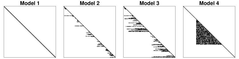
Figure 3: Schematic of four simulation scenarios with $p=100$: (from left to right) Model 1 is strictly banded, Model 2 has small variable bandwidth, Model 3 has large variable bandwidth, and Model 4 is block-diagonal. Black, gray, and white stand for positive, negative, and zero entries, respectively. The proportion of elements that are non-zero is 4%, 6%, 15%, and 26%, respectively.

For all four models and every value of $p$ considered, we verified that Assumptions A3 and A4 hold and then simulated $n=100$ observations according to each of the four models based on Assumption A1.

5.1 Support Recovery

We first study how well the different estimators identify zeros in the four models above. We generate $n=100$ random samples from each model with $p=200$. The tuning parameter $\lambda\geq 0$ in (5) measures the amount of regularization and determines the sparsity level of the estimator. We use 100 tuning parameter values for each estimator and repeat the simulation 10 times.

Figure 4 shows the sensitivity (fraction of true non-zeros that are correctly recovered) and specificity (fraction of true zeros that are correctly set to zero) of each method parameterized by its tuning parameter (in the case of non-adaptive banding, the parameter is the bandwidth itself, ranging from $0$ to $p-1$). Each set of 10 curves of the same color corresponds to the results of one estimator, and each curve within the set corresponds to the result of one draw from 10 simulations. Curves closer to the upper-right corner indicate better classification performance (the $x+y=1$ line corresponds to random guessing).

The sparsity level of the non-adaptive banding estimator depends only on the pre-specified bandwidth (which is the method’s tuning parameter) and not on the data itself. Consequently, the sensitivity-specificity curves for the non-adaptive banding do not vary across replications when simulating from a particular underlying model. The sparsity levels of the nested lasso and our methods, by contrast, hinge on the data, thus giving a different curve for each replication.

Figure 4: ROC curves showing support recovery when the true $L$ (top-left) is strictly banded, (top-right) has small variable bandwidth, (bottom-left) has large variable bandwidth, and (bottom-right) is block-diagonal, over 10 replications.

In practice, we find that our methods and the nested lasso sometimes produce entries with very small, but non-zero, absolute values. To study support recovery, we set all estimates whose absolute values are below $10^{-10}$ to zero, both in our estimators and the nested lasso.

In Model 1, we observe that all methods considered attain perfect classification accuracy for some value of their tuning parameter. While the non-adaptive approach is guaranteed to do so in this scenario, it is reassuring to see that the more flexible methods can still perfectly recover this sparsity pattern.

In Model 2, we observe that our two methods outperform the nested lasso, which itself, as expected, outperforms the non-adaptive banding method. As the model becomes more challenging (from Model 2 to Model 4), the performances of all four methods start deteriorating. Interestingly, the nested lasso no longer retains its advantage over non-adaptive banding in Models 3 and 4, while the performance advantage of our methods become even more substantial.

The fact that the unweighted version of our method outperforms the weighted version stems from the fact that all models are comparatively sparse for $p=200$, and so the heavier penalty on each row delivered by the unweighted approach recovers the support more easily than the weighted version.

5.2 Estimation Accuracy

We proceed by comparing the estimators in terms of how far $\hat{L}$ is from $L$. To this end, we generate $n=100$ random samples from the four models with $p=50$, $p=100$, and $p=200$. Each method is computed with its tuning parameter selected to maximize the Gaussian likelihood on the validation data in a 5-fold cross-validation. For comparison, we report the estimation accuracy of each estimate in terms of the scaled Frobenius norm $\frac{1}{p}\left\lVert\hat{L}-L\right\rVert_{F}^{2}$, the matrix infinity norm ${\left|\kern-1.07639pt\left|\kern-1.07639pt\left|\hat{L}-L\right|\kern-1.07639pt\right|\kern-1.07639pt\right|}_{\infty}$, the spectral norm ${\left|\kern-1.07639pt\left|\kern-1.07639pt\left|\hat{L}-L\right|\kern-1.07639pt\right|\kern-1.07639pt\right|}_{2}$, and the (scaled) Kullback-Leibler loss $\frac{1}{p}\left[\text{tr}(\Omega^{-1}\hat{\Omega})-\log\det(\Omega^{-1}\hat{\Omega})-p\right]$ (Levina et al., 2008).

The simulation is repeated 50 times, and the results are summarized in Figure 5 through Figure 8. Each figure corresponds to a model, and consists of a 4-by-3 panel layout. Each row corresponds to an error measure, and each column corresponds to a value of $p$.

Figure 5: Estimation accuracy when data are generated from Model 1, which is strictly banded.

Figure 6: Estimation accuracy when data are generated from Model 2, which has small variable bandwidth.

Figure 7: Estimation accuracy when data are generated from Model 3, which has large variable bandwidth.

Figure 8: Estimation accuracy when data are generated from Model 4, which is block-diagonal.

As expected, the non-adaptive banding estimator does better than the other estimators in Model 1. In Models 2, 3, and 4, where bandwidths vary with row, our estimators and the nested lasso outperform non-adaptive banding.

A similar pattern is observed as in support recovery. As the model becomes more complex and $p$ gets larger, the performance of the nested lasso degrades and gradually becomes worse than non-adaptive banding. By contrast, as the estimation problem becomes more difficult, the advantage in performance of our methods becomes more obvious.

We again observe that the unweighted estimator performs better than the weighted one. As shown in Section 4, the overall performance of our method hinges on the underlying model complexity (measured in terms of $\max_{r}K_{r}$) as well as the relative size of $n$ and $p$. When $n$ is relatively small, usually a more constrained method (like the unweighted estimator) is preferred over a more flexible method (like the weighted estimator). So in our simulation setting, it is reasonable to observe that the unweighted method works better. Note that as the underlying $L$ becomes denser (from Model 1 to Model 4), the performance difference between the weighted and the unweighted estimator diminishes. This corroborates our discussion in the end of Section 4 that the performance of the unweighted estimator becomes worse when the underlying model is dense.

6 Applications to Data Examples

In this section, we illustrate the practical merits of our proposed method by applying it to two data examples. We start with an application to genomic data where our method can help model the local correlations along the genome. In Section 6.2 we compare our method with other estimators within the context of a sound recording classification problem.

6.1 An Application to Genomic Data

We consider an application of our estimator to modeling correlation along the genome. Genetic mutations that occur close together on a chromosome are more likely to be co-inherited than mutations that are located far apart (or on separate chromosomes). This leads to local correlations between genetic variants in a population. Biologists refer to this local dependence as linkage disequilibrium (LD). The width of this dependence is known to vary along the genome due to the variable locations of recombination hotspots, which suggests that adaptively banded estimators may be quite suitable in these contexts.

We study HapMap phase 3 data from the International HapMap project (Consortium et al., 2010). The data consist of $n=167$ humans from the YRI (Yoruba in Ibadan, Nigeria) population, and we focus on $p=201$ consecutive tag SNPs on chromosome 22 (after filtering out infrequent sites with minor allele frequency $\leq 10\%$).

While tag SNP data, which take discrete values $\{0,1,2\}$, are non-Gaussian, we argue that our estimator is still sensible to use in this case. First, the parameterization $\Omega=L^{T}L$ does not depend on the Gaussian assumption. Moreover the estimator corresponds to minimizing a penalized Bregman divergence of the log-determinant function (Ravikumar et al., 2011). Furthermore, the least-squares term in (5) can be interpreted as minimizing the prediction error in the linear models (1) while the log terms act as log-barrier functions to impose positive diagonal entries (which ensures that the resulting $\hat{L}$ is a valid Cholesky factor).

To gauge the performance of our estimator on modeling LD, we randomly split the $167$ samples into training and testing sets of sizes $84$ and $83$, respectively. Along a path of tuning parameters with decreasing values, estimators $\hat{L}$ are computed on the training data. To evaluate $\hat{L}$ on a vector $\tilde{x}$ from the test data set, we can compute the error in predicting $\hat{L}_{rr}\tilde{x}_{r}$ using $-\sum_{k=1}^{r-1}\hat{L}_{r,k}\tilde{x}_{k}$ via (1) for each $r$, giving the error

$$\mathrm{err}(\tilde{x})=\frac{1}{p-1}\sum_{r=2}^{p}\left(\hat{L}_{rr}\tilde{x}_{r}+\sum_{k=1}^{r-1}\hat{L}_{rj}\tilde{x}_{k}\right)^{2}.$$ (25)

This quantity (with mean and the standard deviation over test samples) is reported in Figure 9 for our estimator under the two weighting schemes. Recall that the quadratically decaying weights (7) act essentially like the $\ell_{1}$ penalty. For numerical comparison, we also include the result of the estimator with $\ell_{1}$ penalty, which is the CSCS (Convex Sparse Cholesky Selection) method proposed in Khare et al. (2016). For both the non-adaptive banding and the nested lasso methods, we found that their implementations fail to work due to the collinearity of the columns of $\mathbf{X}$.

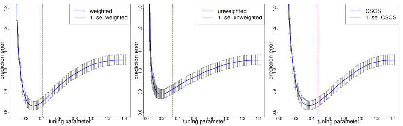
Figure 9: Prediction error (computed on an independent test set) of the weighted (left), unweighted (middle), and CSCS (right) estimators.

Figure 9 shows that our estimators are effective in improving modeling performance over a diagonal estimator (attained when $\lambda$ is sufficiently large) and strongly outperform the plain MLE (as evidenced by the sharp increase in prediction error as $\lambda\to 0$). As expected, the weighted estimator performs very similarly to the CSCS estimator, which uses the $\ell_{1}$ penalty. Both of these perform better than the unweighted one. However, the sparsity pattern obtained by the two penalties are different (as shown in Figure 10).

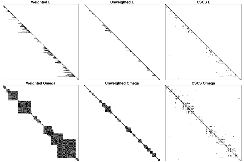
Figure 10: Estimates of linkage disequilibrium with tuning parameters selected by the one-standard-error rule and their corresponding precision matrix estimates.

In Figure 10 we show the recovered signed support of the weighted, unweighted, and CSCS estimators and their corresponding precision matrices. Black, gray, and white stand for positive, negative, and zero entries, respectively. Tuning parameters are chosen using the one-standard-error rule (see, e.g., Hastie et al., 2009). The $r$-th row of the estimated matrix $\hat{L}$ reveals the number of neighboring SNPs necessary for reliably predicting the state of the $r$-th SNP. Interestingly, we see some evidence of small block-like structures in $\hat{L}$, consistent with the hotspot model of recombination as previously described. This regression-based perspective to modeling LD may be a useful complement to the more standard approach, which focuses on raw marginal correlations. Finally, the sparsity recovered by the CSCS estimator, which uses the $\ell_{1}$ penalty, is less easily interpretable, since some entries far from the diagonal are non-zero, losing the notion of ‘local’.

6.2 An Application to Phoneme Classification

In this section, we develop an application of our method to a classification problem described in Hastie et al. (2009). The data contain $n=1717$ continuous speech recordings, which are categorized into two vowel sounds: ‘aa’ ($n_{1}=695$) and ‘ao’ ($n_{2}=1022$). Each observation $(x_{i},y_{i})$ has a predictor $x_{i}\in\mathbb{R}^{p}$ representing the (log) intensity of the sound across $p=256$ frequencies and a class label $y_{i}\in\{1,-1\}$. It may be reasonable to apply our method in this problem since the features are frequencies, which come with a natural ordering

In linear discriminant analysis (LDA), one models the features as multivariate Gaussian conditional on the class: $x_{i}|y_{i}=k\sim N_{p}(\mu^{(k)},\Sigma)$ for $k\in\{1,-1\}$; in quadratic discriminant analysis (QDA), one allows each class to have its own covariance matrix: $x_{i}|y_{i}=k\sim N_{p}(\mu^{(k)},\Sigma^{(k)})$. The LDA/QDA classification rules assign an observation $x\in\mathbb{R}^{p}$ to class $k$ that maximizes $\hat{P}(y=k|x)\propto\hat{P}(x|y=k)\hat{P}(y=k)$, where the estimated probability $\hat{P}(x|y=k)$ is calculated using maximum likelihood estimates $\hat{\mu}^{(k)}$, $\hat{\Sigma}$, and $\hat{\Sigma}^{(k)}$. More precisely, in the ordered case, the resulting class $k$ maximizes the LDA/QDA scores:

$$\delta^{(k)}_{\mathrm{LDA}}(x) =x^{T}\hat{\Omega}\hat{\mu}^{(k)}-\frac{1}{2}(\hat{\mu}^{(k)})^{T}\hat{\Omega}\hat{\mu}^{(k)}+\log\hat{\pi}^{(k)}$$

$$=(\hat{L}x)^{T}\hat{L}\hat{\mu}^{(k)}-\frac{1}{2}\left\lVert\hat{L}\hat{\mu}^{(k)}\right\rVert_{2}^{2}+\log\hat{\pi}^{(k)}$$ (26)

$$\delta^{(k)}_{\mathrm{QDA}}(x) =x^{T}\hat{\Omega}^{(k)}\hat{\mu}^{(k)}-\frac{1}{2}(\hat{\mu}^{(k)})^{T}\hat{\Omega}^{(k)}\hat{\mu}^{(k)}+\log\hat{\pi}^{(k)}$$

$$=(\hat{L}^{(k)}x)^{T}\hat{L}^{(k)}\hat{\mu}^{(k)}-\frac{1}{2}\left\lVert\hat{L}^{(k)}\hat{\mu}^{(k)}\right\rVert_{2}^{2}+\log\hat{\pi}^{(k)}.$$ (27)

Note that it is the precision matrix, not the covariance matrix, that is used in the above scores. In the setting where $p>n$, the MLE of $\Omega$ or $\Omega^{(k)}$ does not exist. A regularized estimate of precision matrix that exploits the natural ordering information can be helpful in this setting.

To demonstrate the use of our estimator in the high-dimensional setting, we randomly split the data into two parts, with $10\%$ of the data assigned to the training set and the remaining $90\%$ of the data assigned to the test set. On the training set, we use 5-fold cross-validation to select the tuning parameter minimizing misclassification error on the validation data. The estimates $\hat{L}$ and $\hat{L}^{(k)}$ are then plugged into (26) and (27) along with $\hat{\mu}^{(k)}=\sum_{i\in{\mathrm{class}\,k}}x_{i}/n^{(k)}$ and $\hat{\pi}^{(k)}=n^{(k)}/n_{\mathrm{train}}$ to calculate the misclassification error in the test set. For comparison, we also include non-adaptive banding, the nested lasso, and CSCS. We compute the classification error (summarized in Table 1), averaged over 10 random train-test splits.

We first observe that, in general, the adaptive methods perform better than the non-adaptive one (which assumes a fixed bandwidth). It is again found that the performance of the weighted estimator is very similar to the one using $\ell_{1}$ penalty (i.e., the CSCS method). And our results are comparable to the nested lasso both in LDA and QDA. Interestingly, we find that the weighted estimator does better in LDA while the unweighted estimator performs better in QDA. The reason, we suspect, is that QDA requires the estimation of more parameters than LDA and therefore favors more constrained methods like the unweighted estimator, which more strongly discourages non-zeros from being far from the diagonal than the weighted one.

	Unweighted	Weighted	Nested Lasso	Non-adaptive	CSCS
LDA	0.271	0.246	0.250	0.268	0.245
QDA	0.232	0.256	0.221	0.246	0.267

Table 1: Average test data classification error rate of discriminant analysis of phoneme data

An R (R Core Team, 2016) package, named varband, is available on CRAN, implementing our estimator. The estimation is very fast with core functions coded in C++, allowing us to solve large-scale problems in substantially less time than is possible with the R-based implementation of the nested lasso.

7 Conclusion

We have presented a new flexible method for learning local dependence in the setting where the elements of a random vector have a known ordering. The model amounts to sparse estimation of the inverse of the Cholesky factor of the covariance matrix with variable bandwidth. Our method is based on a convex formulation that allows it to simultaneously yield a flexible adaptively-banded sparsity pattern, enjoy efficient computational algorithms, and be studied theoretically. To our knowledge, no previous method has all these properties. We show how the matrix estimation problem can be decomposed into independent row estimation problems, each of which can be solved via an ADMM algorithm having efficient updates. We prove that our method recovers the signed support of the true Cholesky factor and attains estimation consistency rates in several matrix norms under assumptions as mild as those in linear regression problems. Simulation studies show that our method compares favorably to two pre-existing estimators in the ordered setting, both in terms of support recovery and in terms of estimation accuracy. Through a genetic data example, we illustrate how our method may be applied to model the local dependence of genetic variations in genes along a chromosome. Finally, we illustrate that our method has favorable performance in a sound recording classification problem.

Appendix A Decoupling Property

Let $S=\frac{1}{n}\mathbf{X}^{T}\mathbf{X}\in\mathbb{R}^{p\times p}$ be the sample covariance matrix. Then the estimator (5) is the solution to the following minimization problem:

$$\min_{\begin{subarray}{c}L:L_{rr}>0\\ L_{rk}=0\text{ for }r<k\end{subarray}}\left\{-2\sum_{r=1}^{p}\log L_{rr}+\operatorname{tr}(SL^{T}L)+\lambda\sum_{r=2}^{p}\sum_{\ell=1}^{r-1}\sqrt{\sum_{m=1}^{\ell}w_{\ell m}^{2}L_{rm}^{2}}\right\}.$$

First note that under the lower-triangular constraint

$$\operatorname{tr}\left(SL^{T}L\right)=\frac{1}{n}\sum_{r=1}^{p}\operatorname{tr}\left(\mathbf{X}L_{\cdot r}^{T}L_{r\cdot}\mathbf{X}^{T}\right)=\frac{1}{n}\sum_{r=1}^{p}\left\lVert\mathbf{X}L_{\cdot r}^{T}\right\rVert_{2}^{2}=\frac{1}{n}\sum_{r=1}^{p}\left\lVert\mathbf{X}_{1:r}L_{1:r,r}^{T}\right\rVert_{2}^{2},$$

where $\mathbf{X}_{1:r}$ is a matrix of the first $r$ columns of $\mathbf{X}$. Thus

$$-2\sum_{r=1}^{p}\log L_{rr}+\operatorname{tr}(SL^{T}L)+\lambda\sum_{r=2}^{p}\sum_{\ell=1}^{r-1}\sqrt{\sum_{m=1}^{\ell}w_{\ell m}^{2}L_{rm}^{2}}$$

$$= -2\log L_{11}+\frac{1}{n}\left\lVert\mathbf{X}_{1}L_{11}\right\rVert_{2}^{2}+\sum_{r=2}^{p}\left(-2\log L_{rr}+\frac{1}{n}\left\lVert\mathbf{X}_{1:r}L_{1:r,r}^{T}\right\rVert_{2}^{2}+\lambda\sum_{\ell=1}^{r-1}\sqrt{\sum_{m=1}^{\ell}w_{\ell m}^{2}L_{rm}^{2}}\right).$$

Therefore the original problem can be decoupled into $p$ separate problems. In particular, a solution $\hat{L}$ can be written in a row-wise form with

$$\hat{L}_{11}=\operatorname*{arg\,min}_{L_{11}>0}\left\{-2\log L_{11}+\frac{1}{n}\left\lVert\mathbf{X}_{1}L_{11}\right\rVert_{2}^{2}\right\}=\frac{1}{\sqrt{S_{11}}},$$

and for $r=2,\ldots,p$,

$$\hat{L}^{T}_{1:r,r}=\operatorname*{arg\,min}_{\beta\in\mathbb{R}^{r}:\beta_{r}>0}\left\{-2\log\beta_{r}+\frac{1}{n}\left\lVert\mathbf{X}_{1:r}\beta\right\rVert_{2}^{2}+\lambda\sum_{\ell=1}^{r-1}\sqrt{\sum_{m=1}^{\ell}w_{\ell m}^{2}\beta_{m}^{2}}\right\}.$$

Appendix B A Closed-Form Solution to (9)

The objective function in (9) is a smooth function. Taking the derivative with respect to $\beta$ and setting to zero gives the following system of equations:

$$-2\frac{1}{\beta_{r}}\mathbf{e}_{r}+\frac{2}{n}\mathbf{X}_{1:r}^{T}\mathbf{X}_{1:r}\beta+u^{(t-1)}+\rho\left(\beta-\gamma^{(t-1)}\right)=\mathbf{0}.$$

Letting $S^{(r)}=\frac{1}{n}\mathbf{X}_{1:r}^{T}\mathbf{X}_{1:r}$, then the equations above can be further decomposed into

$$-\frac{2}{\beta_{r}}+\left(2S^{(r)}_{rr}+\rho\right)\beta_{r}+2S^{(r)}_{r,-r}\beta_{-r}+u^{(t-1)}_{r}-\rho\gamma^{(t-1)}_{r}=0,$$

$$\left(2S^{(r)}_{-r,-r}+\rho I\right)\beta_{-r}+2S^{(r)}_{-r,r}\beta_{r}+u^{(t-1)}_{-r}-\rho\gamma^{(t-1)}_{-r}=\mathbf{0}.$$

Solving for $\beta_{-r}$ in the second system of equations gives

$$\beta_{-r}=-\left(2S^{(r)}_{-r,-r}+\rho I\right)^{-1}\left(2S^{(r)}_{-r,r}\beta_{r}+u^{(t-1)}_{-r}-\rho\gamma^{(t-1)}_{-r}\right),$$

which is then plugged back in the first equation to give

$$2\frac{1}{\beta_{r}}+A\beta_{r}+B=0,$$

where

$$A=4S^{(r)}_{r,-r}\left(2S^{(r)}_{-r,-r}+\rho I\right)^{-1}S^{(r)}_{-r,r}-2S^{(r)}_{r,r}-\rho,$$

$$B=2S^{(r)}_{r,-r}\left(2S^{(r)}_{-r,-r}+\rho I\right)^{-1}\left(u^{(t-1)}_{-r}-\rho\gamma^{(t-1)}_{-r}\right)-u^{(t-1)}_{r}+\rho\gamma^{(t-1)}_{r}.$$

Solving for $\beta_{r}$ gives the closed-form update.

Appendix C Dual Problem of (10)

Lemma 7.

A dual problem of (10) is

$$\min_{a^{(\ell)}\in\mathbb{R}^{r}}\left\{\left\lVert y^{(t)}-\frac{\lambda}{\rho}\sum_{\ell=1}^{r-1}W^{(\ell)}\ast a^{(\ell)}\right\rVert_{2}^{2}\mathrm{\quad s.t.\quad}\left\lVert\left(a^{(\ell)}\right)_{g_{r,\ell}}\right\rVert_{2}\leq 1,\quad\left(a^{(\ell)}\right)_{g_{r,\ell}^{c}}=0\right\},$$ (28)

where $y^{(t)}=\beta^{(t)}+\frac{1}{\rho}u^{(t-1)}$. Also, given a solution $\hat{a}^{(1)},\dots,\hat{a}^{(r-1)}$, the solution to (10) can be written as

$$\gamma^{(t)}=y^{(t)}-\frac{\lambda}{\rho}\sum_{\ell=1}^{r-1}W^{(\ell)}\ast\hat{a}^{(\ell)}.$$ (29)

Proof.

Note that

$$\sqrt{\sum_{m=1}^{\ell}w_{\ell m}^{2}\gamma_{m}^{2}} =\left\lVert\left(W^{(\ell)}\ast\gamma\right)_{g_{r,\ell}}\right\rVert_{2}$$

$$=\max\left\{\left<W^{(\ell)}\ast a^{(\ell)},\gamma\right>,\mathrm{\quad s.t.\quad}\left\lVert\left(a^{(\ell)}\right)_{g_{r,\ell}}\right\rVert_{2}\leq 1,\quad\left(a^{(\ell)}\right)_{g_{r,\ell}^{c}}=0\right\}.$$

Thus, the minimization problem in (10) becomes

$$\min_{\gamma}\left\{\frac{1}{2}\left\lVert\gamma-y^{(t)}\right\rVert_{2}^{2}+\frac{\lambda}{\rho}\sum_{\ell=1}^{r-1}\left\lVert\left(W^{(\ell)}\ast\gamma\right)_{g_{r,\ell}}\right\rVert_{2}\right\}$$

$$= \min_{\gamma}\left\{\max_{a^{(\ell)}}\left\{\frac{1}{2}\left\lVert\gamma-y^{(t)}\right\rVert_{2}^{2}+\frac{\lambda}{\rho}\sum_{\ell=1}^{r-1}\left<W^{(\ell)}\ast a^{(\ell)},\gamma\right>,\left\lVert\left(a^{(\ell)}\right)_{g_{r,\ell}}\right\rVert_{2}\leq 1,\left(a^{(\ell)}\right)_{g_{r,\ell}^{c}}=0\right\}\right\}$$

$$= \max_{a^{(\ell)}}\left\{\min_{\gamma}\left\{\frac{1}{2}\left\lVert\gamma-y^{(t)}\right\rVert_{2}^{2}+\frac{\lambda}{\rho}\sum_{\ell=1}^{r-1}\left<W^{(\ell)}\ast a^{(\ell)},\gamma\right>,\left\lVert\left(a^{(\ell)}\right)_{g_{r,\ell}}\right\rVert_{2}\leq 1,\left(a^{(\ell)}\right)_{g_{r,\ell}^{c}}=0\right\}\right\},$$

where $y^{(t)}=\beta^{(t)}+\frac{1}{\rho}u^{(t-1)}$. We solve the inner minimization problem by setting the derivative to zero,

$$\gamma-y^{(t)}+\frac{\lambda}{\rho}\sum_{\ell=1}^{r-1}W^{(\ell)}\ast a^{(\ell)}=0,$$

which gives the primal-dual relation,

$$\gamma=-\frac{\lambda}{\rho}\sum_{\ell=1}^{r-1}W^{(\ell)}\ast a^{(\ell)}+y^{(t)}.$$

Using this gives

$$\min_{\gamma} \left\{\frac{1}{2}\left\lVert\gamma-y^{(t)}\right\rVert_{2}^{2}+\frac{\lambda}{\rho}\sum_{\ell=1}^{r-1}\left\lVert\left(W^{(\ell)}\ast\gamma\right)_{g_{r,\ell}}\right\rVert_{2}\right\}$$

$$=\max_{a^{(\ell)}} \left\{\frac{1}{2}\left\lVert-\frac{\lambda}{\rho}\sum_{\ell=1}^{r-1}W^{(\ell)}\ast a^{(\ell)}\right\rVert_{2}^{2}+\frac{\lambda}{\rho}\sum_{\ell=1}^{r-1}\left<W^{(\ell)}\ast a^{(\ell)},-\frac{\lambda}{\rho}\sum_{\ell=1}^{r-1}W^{(\ell)}\ast a^{(\ell)}+y^{(t)}\right>\right.$$

$$\left.\mathrm{\quad s.t.\quad}\left\lVert\left(a^{(\ell)}\right)_{g_{r,\ell}}\right\rVert_{2}\leq 1,\quad\left(a^{(\ell)}\right)_{g_{r,\ell}^{c}}=0\right\}$$

$$=\min_{a^{(\ell)}} \left\{\left\lVert y^{(t)}-\frac{\lambda}{\rho}\sum_{\ell=1}^{r-1}W^{(\ell)}\ast a^{(\ell)}\right\rVert_{2}^{2}\mathrm{\quad s.t.\quad}\left\lVert\left(a^{(\ell)}\right)_{g_{r,\ell}}\right\rVert_{2}\leq 1,\quad\left(a^{(\ell)}\right)_{g_{r,\ell}^{c}}=0\right\}.$$

∎

Algorithm 3 BCD on the dual problem (28)

1:Let $y^{(t)}=\beta^{(t)}+\frac{1}{\rho}u^{(t-1)}$

2:Initialize $\hat{a}^{(\ell)}\leftarrow 0$ for all $\ell=1,\cdots,r-1$  

3:for $\ell=1,\cdots,r-1$ do

4:     $\hat{z}^{(\ell)}\leftarrow y^{(t)}-\frac{\lambda}{\rho}\sum_{k=1}^{r-1}W^{(k)}\ast\hat{a}^{(k)}$  Find a root $\hat{\nu}_{\ell}$ that satisfies

$$h_{\ell}(\nu):=\sum_{m=1}^{\ell}\frac{w_{\ell m}^{2}}{\left(w_{\ell m}^{2}+\nu\right)^{2}}\left(\hat{z}^{(\ell)}_{m}\right)^{2}=\frac{\lambda^{2}}{\rho^{2}}$$ (30)

5:     for $m=1,\cdots,\ell$ do

6:         $\hat{a}^{(\ell)}_{m}\leftarrow\frac{w_{\ell m}}{\frac{\lambda}{\rho}\left(w_{\ell m}^{2}+\left[\hat{\nu}_{\ell}\right]_{+}\right)}\hat{z}^{(\ell)}_{m}$        

7:return $\left\{\hat{a}^{(\ell)}\right\}$ as a solution to (28)  

8:return $\gamma^{(t)}=y^{(t)}-\frac{\lambda}{\rho}\sum_{\ell=1}^{r-1}W^{(\ell)}\ast\hat{a}^{(\ell)}$ as a solution to (10)  

Appendix D Elliptical Projection

We adapt the same procedure as in Appendix B of Bien et al. (2016) to update one $a^{(\ell)}$ in Algorithm (3). By (10) we need to solve a problem of the form

$$\min_{a\in\mathbb{R}^{\ell}}\left\lVert\hat{z}^{(\ell)}-\tau Da\right\rVert_{2}^{2}\mathrm{\quad s.t.\quad}\left\lVert a\right\rVert_{2}\leq 1,$$

where $\tau=\frac{\lambda}{\rho}$ and $D=\mathrm{diag}(w_{\ell m})_{m\leq\ell}\in\mathbb{R}^{\ell\times\ell}$. If $\left\lVert D^{-1}\hat{z}^{(\ell)}\right\rVert_{2}\leq\tau$, then clearly $\hat{a}=\frac{1}{\tau}D^{-1}\hat{z}^{(\ell)}$. Otherwise, we use the Lagrangian multiplier method to solve the constrained minimization problem above. Specifically, we find a stationary point of

$$\mathcal{L}\left(a,\nu\right)=\left\lVert\hat{z}^{(\ell)}-\tau Da\right\rVert_{2}^{2}+\nu\tau^{2}\left(\left\lVert a\right\rVert_{2}^{2}-1\right).$$

Taking the derivative with respect to $a$ and set it equal to zero, we have

$$\hat{a}_{m}=\frac{w_{\ell m}}{\tau(w_{\ell m}^{2}+\hat{\nu})}\hat{z}^{(\ell)}_{m},$$

for each $m\leq\ell$, and $\hat{\nu}$ is such that $\left\lVert\hat{a}\right\rVert_{2}=1$, which means it satisfies (30). By observing that $h_{\ell}(\nu)$ is a decreasing function of $\nu$ and $w_{\ell\ell}=\max_{m\leq\ell}w_{\ell m}$, following Appendix B of Bien et al. (2016), we obtain lower and upper bounds for $\hat{\nu}$:

$$\left[\frac{1}{\tau}\left\lVert D\hat{z}^{(\ell)}\right\rVert_{2}-w_{\ell\ell}^{2}\right]_{+}\leq\hat{\nu}\leq\frac{1}{\tau}\left\lVert D\hat{z}^{(\ell)}\right\rVert_{2},$$

which can be used as an initial interval for finding $\hat{\nu}$ using Newton’s method. In practice, we usually find $\hat{\nu}$ from the equation $\frac{1}{h(\nu)}=\tau^{-2}$ for better numerical stability.

We end this section with a characterization of the solution to (10), which says that the solution can be written as $\gamma^{(t)}=y^{(t)}\ast\hat{t}$, where $\hat{t}$ is some data-dependent vector in $\mathbb{R}^{r}$.

Theorem 8.

A solution to (10) can be written as $\gamma^{(t)}=y^{(t)}\ast\hat{g}$, where the data-dependent vector $\hat{g}\in\mathbb{R}^{r}$ is given by

$$\hat{g}_{m}=\prod_{\ell=m}^{r-1}\frac{\left[\hat{\nu}_{\ell}\right]_{+}}{w_{\ell m}^{2}+\left[\hat{\nu}_{\ell}\right]_{+}}$$

and $\hat{g}_{r}=1$, where $\hat{\nu}_{\ell}$ satisfies $\tau^{2}=\sum_{m=1}^{\ell}\frac{w_{\ell m}^{2}}{\left(w_{\ell m}^{2}+\nu\right)^{2}}\left(\hat{z}^{(\ell)}_{m}\right)^{2}$.

Proof.

By Jenatton et al. (2011), we can get a solution to (10) in a single pass as described in Algorithm 3. If we start from $\hat{z}^{(1)}=y^{(t)}$, then for $\ell=1,\cdots,r-1$ and each $m\leq\ell$,

$$\hat{z}^{(\ell+1)}_{m}=\hat{z}^{(\ell)}_{m}-\tau w_{\ell m}\hat{a}^{(\ell)}_{m}=\frac{\left[\hat{\nu}_{\ell}\right]_{+}}{w_{\ell m}^{2}+\left[\hat{\nu}_{\ell}\right]_{+}}\hat{z}^{(\ell)}_{m}.$$

By (29), $\gamma^{(t)}=\hat{z}^{(r-1)}$, and the result follows. ∎

A key observation from this characterization is that a banded sparsity pattern is induced in solving (10), which in turn implies the same property of the output of Algorithm 1.

Corollary 9.

A solution $\gamma^{(t)}$ to (10) has banded sparsity, i.e., $\left(\gamma^{(t)}\right)_{1:\hat{J}}=0$ for $\hat{J}=\max\left\{\ell:\hat{\nu}_{\ell}\leq 0\right\}$.

Appendix E Uniqueness of the Sparse Row Estimator

Lemma 10.

(Optimality condition) For any $\lambda>0$ and a $n$-by-$p$ sample matrix $\mathbf{X}$, $\hat{\beta}$ is a solution to the problem

$$\min_{\beta\in\mathbb{R}^{r}}\left\{-2\log\beta_{r}+\frac{1}{n}\left\lVert\mathbf{X}_{1:r}\beta\right\rVert_{2}^{2}+\lambda\sum_{\ell=1}^{r-1}\sqrt{\sum_{m=1}^{\ell}w_{\ell m}^{2}\beta_{m}^{2}}\right\}$$

if and only if there exist $\hat{a}^{(\ell)}\in\mathbb{R}^{r}$ for $\ell=1,\dots,r-1$ such that

$$-\frac{2}{\hat{\beta}_{r}}\mathbf{e}_{r}+\frac{2}{n}\mathbf{X}_{1:r}^{T}\mathbf{X}_{1:r}\hat{\beta}+\lambda\sum_{\ell=1}^{r-1}W^{(\ell)}\ast\hat{a}^{(\ell)}=0$$ (31)

with $\left(\hat{a}^{(\ell)}\right)_{g_{r,\ell}^{c}}=0$, $\left(\hat{a}^{(\ell)}\right)_{g_{r,\ell}}=\frac{\left(W^{(\ell)}\ast\hat{\beta}\right)_{g_{r,\ell}}}{\left\|\left(W^{(\ell)}\ast\hat{\beta}\right)_{g_{r,\ell}}\right\|_{2}}$ for $\hat{\beta}_{g_{r,\ell}}\neq 0$ and $\left\|\left(\hat{a}^{(\ell)}\right)_{g_{r,\ell}}\right\|_{2}\leq 1$ for $\hat{\beta}_{g_{r,\ell}}=0$.

Lemma 11.

Take $\hat{\beta}$ and $\hat{a}^{(\ell)}$ as in the previous lemma. Suppose that

$$\left\|\left(\hat{a}^{(\ell)}\right)_{g_{r,\ell}}\right\|_{2}<1\quad\quad\text{ for }\quad\ell=1,\dots,J(\hat{\beta})$$

then for any other solution $\tilde{\beta}$ to (8), it is as sparse as $\hat{\beta}$ if not more. In other words,

$$K(\tilde{\beta})\leq\hat{K}_{r}.$$

Lemma 12.

(Uniqueness) Under the conditions of the previous lemma, let $\hat{\mathcal{S}}=\left\{i:\hat{\beta}_{i}\neq 0\right\}$. If $\mathbf{X}_{\hat{\mathcal{S}}}$ has full column rank (i.e., $\operatorname{rank}\left(\mathbf{X}_{\hat{\mathcal{S}}}\right)=|\hat{\mathcal{S}}|$) then $\hat{\beta}$ is unique.

Proof.

See Appendices J, K, and L. ∎

Appendix F Proof of Theorem 1

We start with introducing notation. From now on we suppress the dependence on $r$ in notation for simplicity. We denote the group structure $g_{\ell}=\left\{1,\cdots,\ell\right\}$ for $\ell\leq r$ for each $r=1,\dots,p$. For any vector $\beta\in\mathbb{R}^{r}$, we let $\beta_{g_{\ell}}\in\mathbb{R}^{\ell}$ be the vector with elements $\left\{\beta_{m}:m\leq\ell\right\}$. We also introduce the weight vector $W^{(\ell)}\in\mathbb{R}^{p}$ with $\left(W^{(\ell)}\right)_{m}=w_{\ell m}$ where $w_{\ell m}$ can be defined as in (7) or $w_{\ell m}=1$. Finally recalling from Section 4 the definition of $\mathcal{I}$, we denote $\mathcal{S}=\mathcal{I}\cup\{r\}=\left\{J+1,\dots,r\right\}$ and $\mathcal{S}^{c}=\left\{1,2,\ldots,J\right\}$.

The general idea of the proof depends on the primal-dual witness procedure in Wainwright (2009) and Ravikumar et al. (2011). Considering the original problem (8) for any $r=2,\dots,p$, we construct the primal-dual witness solution pairs $\left(\tilde{\beta},\sum_{\ell=1}^{r-1}W^{(\ell)}\ast\tilde{a}^{(\ell)}\right)$ as follows:

1. Solve the restricted subproblem with the true bandwidth $K=r-1-J$:

   $$\tilde{\beta}=\operatorname*{arg\,min}_{\begin{subarray}{c}\beta_{r}>0\\ \beta_{\mathcal{S}^{c}}=0\end{subarray}}\left\{-2\log\beta_{r}+\frac{1}{n}\left\lVert\mathbf{X}_{1:r}\beta\right\rVert_{2}^{2}+\lambda\sum_{\ell=1}^{r-1}\left\|\left(W^{(\ell)}\ast\beta\right)_{g_{\ell}}\right\|_{2}\right\}.$$

   The solution above can be written as

   $$\tilde{\beta}=\begin{pmatrix}\mathbf{0}_{J}\\ \tilde{\gamma}\end{pmatrix},$$

   where

   $$\tilde{\gamma}=\operatorname*{arg\,min}_{\gamma\in\mathbb{R}^{K+1}}\left\{-2\log\gamma_{K+1}+\frac{1}{n}\left\lVert\mathbf{X}_{\mathcal{S}}\gamma\right\rVert_{2}^{2}+\lambda\sum_{\ell=1}^{K}\left\lVert\left(\tilde{W}^{(\ell)}\ast\gamma\right)_{g_{\ell}}\right\rVert_{2}\right\},$$

   with

   $$\tilde{W}^{(\ell)}=\left(W^{(\ell+J)}\right)_{\mathcal{S}}\quad\iff\quad\sum_{\ell=1}^{K}\left\lVert\left(\tilde{W}^{(\ell)}\ast\gamma\right)_{g_{\ell}}\right\rVert_{2}=\sum_{\ell=J+1}^{r-1}\sqrt{\sum_{m=J+1}^{r-1}w_{\ell m}^{2}\gamma_{m-J}^{2}}.$$

2. By Lemma 10, there exist $\tilde{b}^{(\ell)}\in\mathbb{R}^{K+1}$ for $\ell=1,\dots,K$, such that $\left(\tilde{b}^{(\ell)}\right)_{g_{\ell}^{c}}=0$ and

   $$\left(\tilde{b}^{(\ell)}\right)_{g_{r\ell}}=\frac{\left(\tilde{W}^{(\ell)}\ast\tilde{\gamma}\right)_{g_{\ell}}}{\left\|\left(\tilde{W}^{(\ell)}\ast\tilde{\gamma}\right)_{g_{\ell}}\right\|_{2}},$$

   satisfying

   $$-\frac{2}{\tilde{\gamma}_{K+1}}\mathbf{e}_{K+1}+\frac{2}{n}\mathbf{X}_{\mathcal{S}}^{T}\mathbf{X}_{\mathcal{S}}\tilde{\gamma}+\lambda\sum_{\ell=1}^{K}\tilde{W}^{(\ell)}\ast\tilde{b}^{(\ell)}=0.$$

3. For $\ell=J+1,\dots,r-1$, we let

   $$\tilde{a}^{(\ell)}=\begin{pmatrix}\mathbf{0}_{J}\\ \tilde{b}^{(\ell-J)}\end{pmatrix}.$$

   Then we have $\left(\tilde{a}^{(\ell)}\right)_{g_{\ell}^{c}}=0$, $\left\|\left(\tilde{a}^{(\ell)}\right)_{g_{\ell}}\right\|_{2}\leq 1$, $\left(\tilde{a}^{(\ell)}\right)_{g_{\ell}}=\frac{\left(W^{(\ell)}\ast\tilde{\beta}\right)_{g_{\ell}}}{\left\|\left(W^{(\ell)}\ast\tilde{\beta}\right)_{g_{\ell}}\right\|_{2}}$ for $\tilde{\beta}_{g_{\ell}}\neq 0$.

4. For each $\ell=1,...,J$, we choose $\tilde{a}^{(\ell)}\in\mathbb{R}^{r}$ satisfying

   $$\left(\tilde{a}^{(\ell)}\right)_{\ell^{\prime}}=0\quad\text{ for any }\ell^{\prime}\neq\ell\quad\text{and}\quad\left(\tilde{a}^{(\ell)}\right)_{\ell}=-\frac{2}{\lambda w_{\ell\ell}}\left(S\tilde{\beta}\right)_{\ell}=-\frac{2}{n\lambda}\mathbf{X}^{T}_{\ell}\mathbf{X}_{\mathcal{S}}\tilde{\beta}_{\mathcal{S}}.$$

   By construction and the fact that $w_{\ell\ell}=1$,

   $$\lambda\left(W^{(\ell)}\ast\tilde{a}^{(\ell)}\right)_{\ell}=\lambda w_{\ell\ell}\left(\tilde{a}^{(\ell)}\right)_{\ell}=-2\left(S\tilde{\beta}\right)_{\ell}.$$

   By Lemma 10, $\left\{\tilde{a}^{(\ell)}\right\}$ satisfies the optimality condition (31):

   $$-\frac{2}{\tilde{\beta}_{r}}\mathbf{e}_{r}+\frac{2}{n}\mathbf{X}_{1:r}^{T}\mathbf{X}_{1:r}\tilde{\beta}+\lambda\sum_{\ell=1}^{r-1}W^{(\ell)}\ast\tilde{a}^{(\ell)}=0$$ (32)

5. Verify the strict dual feasibility condition for $\ell=1,...,J$

   $$\left|\frac{2}{n\lambda}\mathbf{X}^{T}_{\ell}\mathbf{X}_{\mathcal{S}}\tilde{\beta}_{\mathcal{S}}\right|=\left|\left(\tilde{a}^{(\ell)}\right)_{\ell}\right|=\left\|\left(\tilde{a}^{(\ell)}\right)_{g_{\ell}}\right\|_{2}<1.$$ (33)

At a high level, steps (a) through (d) construct a pair $\left(\tilde{\beta},\left\{\tilde{a}^{(\ell)}\right\}\right)$ that satisfies the optimality condition (31), but the $\left\{\tilde{a}^{(\ell)}\right\}$ is not necessarily guaranteed to be a member of $\partial\left(P(\tilde{\beta})\right)$. Step (e) does more than verifying the necessary conditions for it to belong to $\partial\left(P(\tilde{\beta})\right)$. The strict dual feasibility condition, once verified, ensures the uniqueness of the solution. Note that by construction in Step (b), $\left\{\tilde{a}^{(\ell)}\right\}$ satisfies dual feasibility conditions for $\ell=J+1,...,r-1$ since $\left\{\tilde{b}^{(\ell)}\right\}$ does, so it remains to verify for $\ell=1,...,J$ (see Step (c)).

For each $\ell=1,...,J$, by the construction in Step (d), $\left(\tilde{a}^{(\ell)}\right)_{g_{\ell}^{c}}=0$. Note that $\tilde{\beta}_{g_{J}}=0$ implies $\tilde{\beta}_{g_{\ell}}=0$. Thus, for $\tilde{a}^{(\ell)}$ to satisfy conditions in Lemma 10, it suffices to show (33).

If the primal-dual witness procedure succeeds, then by construction, the solution $\tilde{\beta}$, whose support is contained in the support of the true $L_{r\cdot}$, is a solution to (8). Moreover, by strict dual feasibility and Lemma 12, we know that $\tilde{\beta}$ is the unique solution $\hat{\beta}$ to the unconstrained problem (8). Therefore, the support of $\hat{\beta}$ is contained in the support of $L_{r\cdot}$.

In the following we adapt the same proof technique as Wainwright (2009) to show that the primal-dual witness succeeds with high probability, from which we first conclude that $K(\hat{\beta})\leq K$.

F.1 Proof of Property 1 in Theorem 1

Proof.

We need to verify the strict dual feasibility (33). By (32),

$$-\frac{2}{\tilde{\beta}_{r}}+\frac{2}{n}\mathbf{X}_{r}^{T}\mathbf{X}_{r}\tilde{\beta}_{r}+\frac{2}{n}\mathbf{X}_{r}^{T}\mathbf{X}_{\mathcal{I}}\tilde{\beta}_{\mathcal{I}}=0,$$ (34)

$$\frac{2}{n}\mathbf{X}_{\mathcal{I}}^{T}\mathbf{X}_{r}\tilde{\beta}_{r}+\frac{2}{n}\mathbf{X}_{\mathcal{I}}^{T}\mathbf{X}_{\mathcal{I}}\tilde{\beta}_{\mathcal{I}}+\lambda\left(\sum_{\ell=1}^{r-1}W^{(\ell)}\ast\tilde{a}^{(\ell)}\right)_{\mathcal{I}}=0.$$ (35)

From (35),

$$\tilde{\beta}_{\mathcal{I}}=-\left(\mathbf{X}_{\mathcal{I}}^{T}\mathbf{X}_{\mathcal{I}}\right)^{-1}\left[\mathbf{X}_{\mathcal{I}}^{T}\mathbf{X}_{r}\tilde{\beta}_{r}+\frac{\lambda n}{2}\left(\sum_{\ell=1}^{r-1}W^{(\ell)}\ast\tilde{a}^{(\ell)}\right)_{\mathcal{I}}\right].$$ (36)

Plugging (36) back into (34) and denoting $\mathbf{C}_{\mathcal{I}}=\mathbf{X}_{\mathcal{I}}\left(\mathbf{X}_{\mathcal{I}}^{T}\mathbf{X}_{\mathcal{I}}\right)^{-1}\left(\sum_{\ell=1}^{r-1}W^{(\ell)}\ast\tilde{a}^{(\ell)}\right)_{\mathcal{I}}$ and $\mathbf{O}_{\mathcal{I}}=\mathbf{I}-\mathbf{X}_{\mathcal{I}}\left(\mathbf{X}_{\mathcal{I}}^{T}\mathbf{X}_{\mathcal{I}}\right)^{-1}\mathbf{X}_{\mathcal{I}}^{T}$ as the orthogonal projection matrix onto the orthogonal complement of the column space of $\mathbf{X}_{\mathcal{I}}$, we have

$$-\frac{2}{\tilde{\beta}_{r}}+\frac{2}{n}\mathbf{X}_{r}^{T}\mathbf{O}_{\mathcal{I}}\mathbf{X}_{r}\tilde{\beta}_{r}-\lambda\mathbf{X}_{r}^{T}\mathbf{C}_{\mathcal{I}}=0,$$

which implies that

$$\tilde{\beta}_{r}=\frac{\frac{\lambda}{2}\mathbf{X}^{T}_{r}\mathbf{C}_{\mathcal{I}}+\sqrt{\frac{\lambda^{2}}{4}\left(\mathbf{X}^{T}_{r}\mathbf{C}_{\mathcal{I}}\right)^{2}+\frac{4}{n}\mathbf{X}_{r}^{T}\mathbf{O}_{\mathcal{I}}\mathbf{X}_{r}}}{\frac{2}{n}\mathbf{X}_{r}^{T}\mathbf{O}_{\mathcal{I}}\mathbf{X}_{r}}$$ (37)

and that

$$\left(\tilde{a}^{(\ell)}\right)_{\ell} =-\frac{2}{n\lambda}\mathbf{X}^{T}_{\ell}\mathbf{X}_{\mathcal{S}}\tilde{\beta}_{\mathcal{S}}=-\frac{2}{n\lambda}\mathbf{X}^{T}_{\ell}\mathbf{X}_{r}\tilde{\beta}_{r}-\frac{2}{n\lambda}\mathbf{X}^{T}_{\ell}\mathbf{X}_{\mathcal{I}}\tilde{\beta}_{\mathcal{I}}$$

$$=-\frac{2}{n\lambda}\mathbf{X}^{T}_{\ell}\mathbf{X}_{r}\tilde{\beta}_{r}+\frac{2}{n\lambda}\mathbf{X}^{T}_{\ell}\mathbf{X}_{\mathcal{I}}\left(\mathbf{X}_{\mathcal{I}}^{T}\mathbf{X}_{\mathcal{I}}\right)^{-1}\left[\mathbf{X}_{\mathcal{I}}^{T}\mathbf{X}_{r}\tilde{\beta}_{r}+\frac{\lambda n}{2}\left(\sum_{\ell=1}^{r-1}W^{(\ell)}\ast\tilde{a}^{(\ell)}\right)_{\mathcal{I}}\right]$$

$$=-\frac{2}{n\lambda}\mathbf{X}^{T}_{\ell}\left[\mathbf{I}-\mathbf{X}_{\mathcal{I}}\left(\mathbf{X}_{\mathcal{I}}^{T}\mathbf{X}_{\mathcal{I}}\right)^{-1}\mathbf{X}_{\mathcal{I}}^{T}\right]\mathbf{X}_{r}\tilde{\beta}_{r}+\mathbf{X}^{T}_{\ell}\mathbf{X}_{\mathcal{I}}\left(\mathbf{X}_{\mathcal{I}}^{T}\mathbf{X}_{\mathcal{I}}\right)^{-1}\left(\sum_{\ell=1}^{r-1}W^{(\ell)}\ast\tilde{a}^{(\ell)}\right)_{\mathcal{I}}$$

$$=\mathbf{X}_{\ell}^{T}\left[\mathbf{C}_{\mathcal{I}}-\mathbf{O}_{\mathcal{I}}\left(\frac{2}{n\lambda}\mathbf{X}_{r}\tilde{\beta}_{r}\right)\right].$$ (38)

Conditioning on $\mathbf{X}_{\mathcal{I}}$, we can decompose $\mathbf{X}_{r}$ and $\mathbf{X}_{\ell}$ as

$$\mathbf{X}_{r}^{T}=\Sigma_{r\mathcal{I}}\left(\Sigma_{\mathcal{I}\mathcal{I}}\right)^{-1}\mathbf{X}^{T}_{\mathcal{I}}+E^{T}_{r},$$ (39)

$$\mathbf{X}_{\ell}^{T}=\Sigma_{\ell\mathcal{I}}\left(\Sigma_{\mathcal{I}\mathcal{I}}\right)^{-1}\mathbf{X}^{T}_{\mathcal{I}}+E^{T}_{\ell},$$

where $E_{r}\sim N\left(\mathbf{0}_{n},\theta^{(r)}_{r}\mathbf{I}_{n\times n}\right)$ and $E_{\ell}\sim N\left(\mathbf{0}_{n},\theta^{(\ell)}_{r}\mathbf{I}_{n\times n}\right)$, and $\theta_{r}^{(\ell)}$ and $\theta_{r}^{(r)}$ are defined in Section 4. Then

$$\mathbf{X}^{T}_{\ell}\mathbf{O}_{\mathcal{I}}=E_{\ell}^{T}\mathbf{O}_{\mathcal{I}}\quad\text{ and }\quad\mathbf{O}_{\mathcal{I}}\mathbf{X}_{r}=\mathbf{O}_{\mathcal{I}}E_{r},$$

and from (38)

$$\left(\tilde{a}^{(\ell)}\right)_{\ell} =E_{\ell}^{T}\left[\mathbf{C}_{\mathcal{I}}-\mathbf{O}_{\mathcal{I}}\left(\frac{2}{n\lambda}E_{r}\tilde{\beta}_{r}\right)\right]+\Sigma_{\ell\mathcal{I}}\left(\Sigma_{\mathcal{I}\mathcal{I}}\right)^{-1}\left(\sum_{\ell=1}^{r-1}W^{(\ell)}\ast\tilde{a}^{(\ell)}\right)_{\mathcal{I}}$$

$$:=R^{(\ell)}+F^{(\ell)}.$$ (40)

We first bound $\max_{\ell}\left|F^{(\ell)}\right|$. Note that

$$\left\|\left(\sum_{\ell=1}^{r-1}W^{(\ell)}\ast\tilde{a}^{(\ell)}\right)_{\mathcal{I}}\right\|_{\infty}=\left\|\left(\sum_{\ell=J+1}^{r-1}W^{(\ell)}\ast\tilde{a}^{(\ell)}\right)_{\mathcal{I}}\right\|_{\infty}=\max_{m\in\mathcal{I}}\left|\sum_{\ell=m}^{r-1}w_{\ell m}\left(\tilde{a}^{(\ell)}\right)_{m}\right|$$

$$\leq \max_{m\in\mathcal{I}}\sum_{\ell=m}^{r-1}w_{\ell m}\left|\left(\tilde{a}^{(\ell)}\right)_{m}\right|\leq\max_{m\in\mathcal{I}}\sum_{\ell=m}^{r-1}\frac{1}{\left(\ell-m+1\right)^{2}}\leq\sum_{k=1}^{\infty}\frac{1}{k^{2}}=\frac{\pi^{2}}{6},$$ (41)

where we used $\left\lVert\tilde{a}^{(\ell)}\right\rVert_{\infty}\leq\left\lVert\tilde{a}^{(\ell)}\right\rVert_{2}\leq 1$. Therefore, by Assumption A3,

$$\max_{1\leq\ell\leq J}\left|\Sigma_{\ell\mathcal{I}}\left(\Sigma_{\mathcal{I}\mathcal{I}}\right)^{-1}\left(\sum_{\ell=1}^{r-1}W^{(\ell)}\ast\tilde{a}^{(\ell)}\right)_{\mathcal{I}}\right|\leq 1-\alpha.$$

To give a bound on the random quantity $\left|R^{(\ell)}\right|$, we first state a general result that will be used multiple times later in the proof.

Lemma 13.

Consider the term $E_{j}^{T}\eta$ where $\eta\in\mathbb{R}^{n}$ is a random vector depending on $\mathbf{X}_{\mathcal{I}}$ and $\mathbf{X}_{r}$ and $E_{j}\sim N\left(\mathbf{0}_{n},\theta_{r}^{(j)}\mathbf{I}_{n\times n}\right)$ for $j=1,\dots,J,r$. If for some $\bar{Q}\geq 0$

$$\mathrm{P}\left[\mathrm{Var}\left(E_{j}^{T}\eta\Big{|}\mathbf{X}_{\mathcal{I}},\mathbf{X}_{r}\right)\geq\bar{Q}\right]\leq\bar{p}$$

then for any $a>0$,

$$\mathrm{P}\left[\left|E_{j}^{T}\eta\right|\geq a\right]\leq 2\exp\left(-\frac{a^{2}}{2\bar{Q}}\right)+\bar{p}$$

Proof.

Define the event

$$\bar{\mathcal{B}}=\left\{\mathrm{Var}\left(E_{j}^{T}\eta\Big{|}\mathbf{X}_{\mathcal{I}}\right)\geq\bar{Q}\right\}.$$

Now for any $a$ and conditioned on $\mathbf{X}_{\mathcal{I}}$ and $\mathbf{X}_{r}$,

$$\mathrm{P}\left[E_{j}^{T}\eta\geq a\right]\leq\mathrm{P}\left[E_{j}^{T}\eta\geq a\Big{|}\bar{\mathcal{B}}^{c}\right]+\mathrm{P}\left[\bar{\mathcal{B}}\right]\leq\mathrm{P}\left[E_{j}^{T}\eta\geq a\Big{|}\bar{\mathcal{B}}^{c}\right]+\bar{p}.$$

Conditioned on $\bar{\mathcal{B}}^{c}$, the variance of $E_{j}^{T}\eta$ is at most $\bar{Q}$. So by standard Gaussian tail bounds, we have

$$\mathrm{P}\left[E_{j}^{T}\eta\geq a\Big{|}\bar{\mathcal{B}}^{c}\right]=\mathrm{E}\left[\mathrm{P}\left(E_{j}^{T}\eta\geq a\Big{|}\mathbf{X}_{\mathcal{I}},\mathbf{X}_{r}\right)\Big{|}\bar{\mathcal{B}}^{c}\right]\leq\mathrm{E}\left[2\exp\left(-\frac{a^{2}}{2\bar{Q}}\right)\Big{|}\bar{\mathcal{B}}^{c}\right]\leq 2\exp\left(-\frac{a^{2}}{2\bar{Q}}\right).$$

∎

Then note that $\mathrm{Var}\left(E_{i\ell}\right)=\theta_{r}^{(\ell)}\leq\theta_{r}$ for $i=1,\dots,n$. Now conditioned on both $\mathbf{X}_{\mathcal{I}}$ and $\mathbf{X}_{r}$, $R^{(\ell)}$ is zero-mean with variance at most

$$\mathrm{Var} \left(R^{(\ell)}\Big{|}\mathbf{X}_{\mathcal{I}}\right)$$

$$\leq \theta_{r}\left\lVert\mathbf{C}_{\mathcal{I}}-\mathbf{O}_{\mathcal{I}}\left(\frac{2}{n\lambda}E_{r}\tilde{\beta}_{r}\right)\right\rVert^{2}_{2}=\theta_{r}\left\{\mathbf{C}_{\mathcal{I}}^{T}\mathbf{C}_{\mathcal{I}}+\left\lVert\mathbf{O}_{\mathcal{I}}\left(\frac{2}{n\lambda}E_{r}\tilde{\beta}_{r}\right)\right\rVert^{2}_{2}\right\}$$

$$= \theta_{r}\left\{\frac{1}{n}\left(\sum_{\ell=1}^{r-1}W^{(\ell)}\ast\tilde{a}^{(\ell)}\right)^{T}_{\mathcal{I}}\left(\frac{1}{n}\mathbf{X}_{\mathcal{I}}^{T}\mathbf{X}_{\mathcal{I}}\right)^{-1}\left(\sum_{\ell=1}^{r-1}W^{(\ell)}\ast\tilde{a}^{(\ell)}\right)_{\mathcal{I}}+\frac{4\tilde{\beta}^{2}_{r}\left\lVert\mathbf{O}_{\mathcal{I}}E_{r}\right\rVert^{2}_{2}}{n^{2}\lambda^{2}}\right\}$$

$$:= \theta_{r}M_{n},$$

where the first equality holds from Pythagorean identity. The next lemma bounds the random scaling $M_{n}$.

Lemma 14.

For $\varepsilon\in\left(0,\frac{1}{2}\right)$, denote

$$\bar{M}_{n}\left(\varepsilon\right):=\frac{3\kappa^{2}\pi^{2}}{2}\frac{K}{n}+\frac{1}{\theta_{r}^{(r)}\left(n-K\right)\left(1-\varepsilon\right)}+\frac{16}{n\lambda^{2}},$$

then

$$\mathrm{P}\left[M_{n}\geq\bar{M}_{n}\left(\varepsilon\right)\Big{|}\mathbf{X}_{\mathcal{I}}\right]\leq 7\exp\left(-n\min\left\{\frac{\alpha^{2}}{3\theta_{r}^{(r)}\kappa^{2}\pi^{2}K},\frac{\varepsilon^{2}}{4}\left(1-\frac{K}{n}\right)\right\}\right).$$

Proof.

See Appendix M. ∎

Now by Lemma 13 and the union bound,

$$\mathrm{P}\left[\max_{1\leq\ell\leq J}\left|R^{(\ell)}\right|\geq\alpha\right]\leq 2J\exp\left(-\frac{\alpha^{2}}{2\theta_{r}\bar{M}_{n}\left(\varepsilon\right)}\right)+7\exp\left(-c_{3}n\right),$$ (42)

for some constant $c_{3}$ independent of $n$ and $J$. By the assumption that $\frac{K}{n}=o(1)$, we have that $\frac{K}{n}\leq 1-\varepsilon$ for $n$ large enough, thus

$$\bar{M}_{n}\left(\varepsilon\right)\leq\frac{K}{n}\left(\frac{3\kappa^{2}\pi^{2}}{2}+\frac{1}{K\theta_{r}^{(r)}\left(1-\varepsilon\right)^{2}}+\frac{16}{K\lambda^{2}}\right)\leq\frac{K}{n}\left(\frac{3\kappa^{2}\pi^{2}}{2}+\frac{4}{K\theta_{r}^{(r)}}+\frac{16}{K\lambda^{2}}\right).$$

For the exponential term in (42) to have faster decaying rate than the $J$ term, we need

$$\frac{n}{K\log J}>\frac{\theta_{r}}{\alpha^{2}}\left(3\kappa^{2}\pi^{2}+\frac{8}{K\theta_{r}^{(r)}}+\frac{32}{K\lambda^{2}}\right).$$

∎

F.2 Proof of Property 2 in Theorem 1

Next we study the $\ell_{\infty}$ error bound. The following theorem gives an $\ell_{\infty}$ error bound of $\tilde{\beta}$.

Proof.

Let $\delta=\tilde{\beta}-\beta^{\ast}=\tilde{\beta}-\left({L}^{T}\right)_{1:r,r}$ and $\mathcal{W}=S{L}^{T}-\left(L\right)^{-1}$, then from (35) and the fact that $L^{-1}$ is lower-triangular,

$$\delta_{\mathcal{I}}= -\left(\mathbf{X}_{\mathcal{I}}^{T}\mathbf{X}_{\mathcal{I}}\right)^{-1}\left[\mathbf{X}_{\mathcal{I}}^{T}\mathbf{X}_{r}\tilde{\beta}_{r}+\left(\mathbf{X}_{\mathcal{I}}^{T}\mathbf{X}_{\mathcal{I}}\right)\left(L\right)^{T}_{\mathcal{I},r}\right]-\frac{n\lambda}{2}\left(\mathbf{X}_{\mathcal{I}}^{T}\mathbf{X}_{\mathcal{I}}\right)^{-1}\left(\sum_{\ell=1}^{r-1}W^{(\ell)}\ast\tilde{a}^{(\ell)}\right)_{\mathcal{I}}$$

$$= -\left(\frac{1}{n}\mathbf{X}_{\mathcal{I}}^{T}\mathbf{X}_{\mathcal{I}}\right)^{-1}\left[\frac{1}{n}\mathbf{X}_{\mathcal{I}}^{T}\mathbf{X}_{r}\left(\delta_{r}+\beta^{\ast}_{r}\right)+\left(\frac{1}{n}\mathbf{X}_{\mathcal{I}}^{T}\mathbf{X}_{\mathcal{I}}\right)\left(L\right)^{T}_{\mathcal{I},r}\right]$$

$$- \frac{\lambda}{2}\left(\frac{1}{n}\mathbf{X}_{\mathcal{I}}^{T}\mathbf{X}_{\mathcal{I}}\right)^{-1}\left(\sum_{\ell=1}^{r-1}W^{(\ell)}\ast\tilde{a}^{(\ell)}\right)_{\mathcal{I}}$$

$$= -\left(\mathbf{X}_{\mathcal{I}}^{T}\mathbf{X}_{\mathcal{I}}\right)^{-1}\mathbf{X}_{\mathcal{I}}^{T}\mathbf{X}_{r}\delta_{r}-\left(\frac{1}{n}\mathbf{X}_{\mathcal{I}}^{T}\mathbf{X}_{\mathcal{I}}\right)^{-1}\left(S{L}^{T}\right)_{\mathcal{I},r}$$

$$- \frac{\lambda}{2}\left(\frac{1}{n}\mathbf{X}_{\mathcal{I}}^{T}\mathbf{X}_{\mathcal{I}}\right)^{-1}\left(\sum_{\ell=1}^{r-1}W^{(\ell)}\ast\tilde{a}^{(\ell)}\right)_{\mathcal{I}}$$

$$= -\left(\mathbf{X}_{\mathcal{I}}^{T}\mathbf{X}_{\mathcal{I}}\right)^{-1}\mathbf{X}_{\mathcal{I}}^{T}\mathbf{X}_{r}\delta_{r}-\left(\frac{1}{n}\mathbf{X}_{\mathcal{I}}^{T}\mathbf{X}_{\mathcal{I}}\right)^{-1}\mathcal{W}_{\mathcal{I},r}-\frac{\lambda}{2}\left(\frac{1}{n}\mathbf{X}_{\mathcal{I}}^{T}\mathbf{X}_{\mathcal{I}}\right)^{-1}\left(\sum_{\ell=1}^{r-1}W^{(\ell)}\ast\tilde{a}^{(\ell)}\right)_{\mathcal{I}}.$$ (43)

From (34) and the fact that $\left(L^{-1}\right)_{rr}=\frac{1}{L_{rr}}$,

$$-\frac{1}{\tilde{\beta}_{r}}+\frac{1}{n}\mathbf{X}_{r}^{T}\mathbf{X}_{r}\delta_{r}+\frac{1}{n}\mathbf{X}_{r}^{T}\mathbf{X}_{\mathcal{I}}\delta_{\mathcal{I}}+\frac{1}{n}\mathbf{X}_{r}^{T}\mathbf{X}_{r}\beta^{\ast}_{r}+\frac{1}{n}\mathbf{X}_{r}^{T}\mathbf{X}_{\mathcal{I}}\beta^{\ast}_{\mathcal{I}}$$

$$=-\frac{1}{\tilde{\beta}_{r}}+\frac{1}{n}\mathbf{X}_{r}^{T}\mathbf{X}_{r}\delta_{r}+\frac{1}{n}\mathbf{X}_{r}^{T}\mathbf{X}_{\mathcal{I}}\delta_{\mathcal{I}}+\left(S{L}^{T}\right)_{rr}$$

$$=\left(L^{-1}\right)_{rr}-\frac{1}{\tilde{\beta}_{r}}+\frac{1}{n}\mathbf{X}_{r}^{T}\mathbf{X}_{r}\delta_{r}+\frac{1}{n}\mathbf{X}_{r}^{T}\mathbf{X}_{\mathcal{I}}\delta_{\mathcal{I}}+\mathcal{W}_{rr}$$

$$=\frac{\delta_{r}}{L_{rr}\tilde{\beta}_{r}}+\frac{1}{n}\mathbf{X}_{r}^{T}\mathbf{X}_{r}\delta_{r}+\frac{1}{n}\mathbf{X}_{r}^{T}\mathbf{X}_{\mathcal{I}}\delta_{\mathcal{I}}+\mathcal{W}_{rr}=0.$$ (44)

Plugging (43) into (44), we have

$$\frac{\delta_{r}}{L_{rr}\tilde{\beta_{r}}}+\frac{1}{n}\mathbf{X}_{r}^{T}\mathbf{O}_{\mathcal{I}}\mathbf{X}_{r}\delta_{r}=\mathbf{X}_{r}^{T}\mathbf{X}_{\mathcal{I}}\left(\mathbf{X}_{\mathcal{I}}^{T}\mathbf{X}_{\mathcal{I}}\right)^{-1}\mathcal{W}_{\mathcal{I},r}+\frac{\lambda}{2}\mathbf{X}_{r}\mathbf{C}_{\mathcal{I}}-\mathcal{W}_{rr},$$

which implies

$$\delta_{r}=\left(\frac{1}{L_{rr}\tilde{\beta}_{r}}+\frac{1}{n}\mathbf{X}_{r}^{T}\mathbf{O}_{\mathcal{I}}\mathbf{X}_{r}\right)^{-1}\left[\mathbf{X}_{r}^{T}\mathbf{X}_{\mathcal{I}}\left(\mathbf{X}_{\mathcal{I}}^{T}\mathbf{X}_{\mathcal{I}}\right)^{-1}\mathcal{W}_{\mathcal{I},r}+\frac{\lambda}{2}\mathbf{X}_{r}\mathbf{C}_{\mathcal{I}}-\mathcal{W}_{rr}\right].$$

Since $L_{rr}>0$ and $\tilde{\beta}_{r}>0$,

$$|\delta_{r}|\leq \left|\left(\frac{1}{L_{rr}\tilde{\beta}_{r}}+\frac{1}{n}{\mathbf{X}_{r}^{T}\mathbf{O}_{\mathcal{I}}\mathbf{X}_{r}}\right)^{-1}\right|\left(\left|\mathbf{X}_{r}^{T}\mathbf{X}_{\mathcal{I}}\left(\mathbf{X}_{\mathcal{I}}^{T}\mathbf{X}_{\mathcal{I}}\right)^{-1}\mathcal{W}_{\mathcal{I},r}\right|+\left|\frac{\lambda}{2}\mathbf{X}_{r}\mathbf{C}_{\mathcal{I}}\right|+\left|\mathcal{W}_{rr}\right|\right)$$

$$\leq \left|\left(\frac{1}{n}{\mathbf{X}_{r}^{T}\mathbf{O}_{\mathcal{I}}\mathbf{X}_{r}}\right)^{-1}\right|\left(\left|\mathbf{X}_{r}^{T}\mathbf{X}_{\mathcal{I}}\left(\mathbf{X}_{\mathcal{I}}^{T}\mathbf{X}_{\mathcal{I}}\right)^{-1}\mathcal{W}_{\mathcal{I},r}\right|+\left|\frac{\lambda}{2}\mathbf{X}_{r}\mathbf{C}_{\mathcal{I}}\right|+\left|\mathcal{W}_{rr}\right|\right).$$

Now conditioned on $\mathbf{X}_{\mathcal{I}}$, by the decomposition (39), $\left(\frac{1}{n}\mathbf{X}_{r}^{T}\mathbf{O}_{\mathcal{I}}\mathbf{X}_{r}\right)^{-1}=\left(\frac{1}{n}E_{r}^{T}\mathbf{O}_{\mathcal{I}}E_{r}\right)^{-1}=\frac{n}{\left\lVert\mathbf{O}_{\mathcal{I}}E_{r}\right\rVert_{2}^{2}}$. From Lemma 20, it follows that

$$\mathrm{P}\left[\left(\frac{1}{n}\mathbf{X}_{r}^{T}\mathbf{O}_{\mathcal{I}}\mathbf{X}_{r}\right)^{-1}\geq\frac{1}{\theta_{r}^{(r)}}\frac{n}{n-K}\frac{1}{1-\varepsilon}\right]\leq\exp\left(-\frac{1}{4}\left(n-K\right)\varepsilon^{2}\right).$$

Also, by Lemma 19,

$$\mathrm{P}\left[\left|\mathbf{X}_{r}^{T}\mathbf{C}_{\mathcal{I}}\right|\geq 1\right]\leq 2\exp\left(-\frac{n\alpha^{2}}{3\theta_{r}^{(r)}\kappa^{2}\pi^{2}K}\right)+2\exp\left(-\frac{n}{2}\right).$$

To deal with the rest of terms in (44) that involve $\mathcal{W}$, we introduce the following concentration inequality to control its element-wise infinity norm.

Lemma 15.

Let $\mathcal{W}=S{L}^{T}-L^{-1}$. Under Assumptions A4 and A4, there exist constants $C_{1},C_{2},C_{3}>0$ such that for any $0<t\leq 2\kappa$,

$$\mathrm{P}\left[\left\lVert\mathcal{W}\right\rVert_{\infty}>t\right]\leq 2p^{2}\exp\left(-\frac{C_{3}nt^{2}}{\kappa^{2}}\right)+4p\exp\left(-\frac{C_{1}nt}{\kappa^{2}}\right)+4p\exp\left(-C_{2}nt\right).$$

Proof.

See Appendix N. ∎

In terms of the event

$$\mathcal{A}=\left\{\left\lVert\mathcal{W}\right\rVert_{\infty}\leq\lambda\right\},$$

Lemma 15 states that

$$\mathrm{P}\left[\mathcal{A}^{c}\right]\leq 2p^{2}\exp\left(-\frac{C_{3}n\lambda^{2}}{\kappa^{2}}\right)+4p\exp\left(-\frac{C_{1}n\lambda}{\kappa^{2}}\right)+4p\exp\left(-C_{2}n\lambda\right).$$

The next lemma shows that, on the event $\mathcal{A}$ and with the assumption that $\frac{\lambda^{2}}{n}=o(1)$, the term $\left|\mathbf{X}_{r}^{T}\mathbf{X}_{\mathcal{I}}\left(\mathbf{X}_{\mathcal{I}}^{T}\mathbf{X}_{\mathcal{I}}\right)^{-1}\mathcal{W}_{\mathcal{I},r}\right|$ can be bounded by $\lambda$ with high probability.

Lemma 16.

Using the general weigthing scheme (7), we have

$$\mathrm{P}\left[\left|\mathbf{X}_{r}^{T}\mathbf{X}_{\mathcal{I}}\left(\mathbf{X}_{\mathcal{I}}^{T}\mathbf{X}_{\mathcal{I}}\right)^{-1}\mathcal{W}_{\mathcal{I},r}\right|\geq\lambda\Big{|}\mathcal{A}\right]\leq 2\exp\left(-\frac{2n\alpha^{2}}{9\theta_{r}^{(r)}\kappa^{2}K\lambda^{2}}\right)+2\exp\left(-\frac{n}{2}\right).$$

Proof.

Recall that by conditioning on $\mathbf{X}_{\mathcal{I}}$, the decomposition (39) gives

$$\mathbf{X}_{r}^{T}\mathbf{X}_{\mathcal{I}}\left(\mathbf{X}_{\mathcal{I}}^{T}\mathbf{X}_{\mathcal{I}}\right)^{-1}\mathcal{W}_{\mathcal{I},r}=\Sigma_{r\mathcal{I}}\left(\Sigma_{\mathcal{I}\mathcal{I}}\right)^{-1}\mathcal{W}_{\mathcal{I},r}+E^{T}_{r}\mathbf{X}_{\mathcal{I}}\left(\mathbf{X}_{\mathcal{I}}^{T}\mathbf{X}_{\mathcal{I}}\right)^{-1}\mathcal{W}_{\mathcal{I},r}.$$

On the event $\mathcal{A}$, by A3 and (41),

$$\left|\Sigma_{r\mathcal{I}}\left(\Sigma_{\mathcal{I}\mathcal{I}}\right)^{-1}\mathcal{W}_{\mathcal{I},r}\right|\leq{\left|\kern-1.07639pt\left|\kern-1.07639pt\left|\Sigma_{r\mathcal{I}}\left(\Sigma_{\mathcal{I}\mathcal{I}}\right)^{-1}\right|\kern-1.07639pt\right|\kern-1.07639pt\right|}_{\infty}\left\lVert\mathcal{W}_{\mathcal{I},r}\right\rVert_{\infty}\leq\lambda.$$

Note that $\mathrm{Var}\left(E_{ir}\right)=\theta_{r}^{(r)}$ for $i=1,\dots,n$. Let $B^{(r)}:=E_{r}^{T}\mathbf{X}_{\mathcal{I}}\left(\mathbf{X}^{T}_{\mathcal{I}}\mathbf{X}_{\mathcal{I}}\right)^{-1}\mathcal{W}_{\mathcal{I},r}$, then $B^{(r)}$ has mean zero and variance at most

$$\mathrm{Var}\left(B^{(r)}\Big{|}\mathbf{X}_{\mathcal{I}}\right)=\frac{\theta_{r}^{(r)}}{n}\mathcal{W}_{\mathcal{I},r}^{T}\left(\frac{1}{n}\mathbf{X}_{\mathcal{I}}^{T}\mathbf{X}_{\mathcal{I}}\right)^{-1}\mathcal{W}_{\mathcal{I},r}\leq\frac{9\theta_{r}^{(r)}\kappa^{2}K\lambda^{2}}{n},$$

with probability greater than $1-2\exp\left(\frac{n}{2}\right)$. The result follows from Lemma 13. ∎

Putting everything together and choosing the tuning parameter from (13), with a union bound argument and some algebra, we have shown that conditioned on $\mathbf{X}_{\mathcal{I}}$,

$$\mathrm{P}\left[|\delta_{r}|\geq\frac{1}{\theta_{r}^{(r)}}\frac{n}{n-K}\frac{1}{1-\varepsilon}\frac{5}{2}\lambda\right]\leq\mathrm{P}\left[|\delta_{r}|\geq\frac{5}{2\theta_{r}^{(r)}}\lambda\right]\leq\mathrm{P}\left[|\delta_{r}|\geq\frac{5}{2\theta_{r}^{(r)}}\lambda\Big{|}\mathcal{A}\right]+\mathrm{P}\left[\mathcal{A}^{c}\right]$$

$$\leq\exp\left(-\frac{1}{4n}\left(1-\frac{K}{n}\right)\varepsilon^{2}\right)+2\exp\left(-\frac{n\alpha^{2}}{3\theta_{r}\kappa^{2}\pi^{2}K}\right)+2\exp\left(-\frac{2n\alpha^{2}}{9\theta_{r}\kappa^{2}K\lambda^{2}}\right)+4\exp\left(-\frac{n}{2}\right)$$

$$+2p^{2}\exp\left(-\frac{C_{3}n\lambda^{2}}{\kappa^{2}}\right)+4p\exp\left(-\frac{C_{1}n\lambda}{\kappa^{2}}\right)+4p\exp\left(-C_{2}n\lambda\right)$$

$$\leq c_{4}\exp\left(-c_{5}n\right)+\frac{c_{6}}{p},$$ (45)

for some constants $c_{4},c_{5},c_{6},x>0$ that do not depend on $n$ and $p$.

We now consider a bound for $\delta_{\mathcal{I}}$. Recall from (43) that

$$\delta_{\mathcal{I}}=F_{1}+F_{2}$$

where

$$F_{1}= -\left(\mathbf{X}_{\mathcal{I}}^{T}\mathbf{X}_{\mathcal{I}}\right)^{-1}\mathbf{X}_{\mathcal{I}}^{T}\mathbf{X}_{r}\delta_{r},$$

$$F_{2}= -\left(\frac{1}{n}\mathbf{X}_{\mathcal{I}}^{T}\mathbf{X}_{\mathcal{I}}\right)^{-1}\left(\mathcal{W}_{\mathcal{I},r}+\frac{\lambda}{2}\mathbf{D}\right)\quad\text{ with }\quad\mathbf{D}=\left(\sum_{\ell=1}^{r-1}W^{(\ell)}\ast\tilde{a}^{(\ell)}\right)_{\mathcal{I}}.$$

An $\ell_{\infty}$ bound of $F_{2}$ is given by

$$\left\lVert F_{2}\right\rVert_{\infty}\leq\left\lVert\left(\left(\frac{1}{n}\mathbf{X}_{\mathcal{I}}^{T}\mathbf{X}_{\mathcal{I}}\right)^{-1}-\left(\Sigma_{\mathcal{I}\mathcal{I}}\right)^{-1}\right)\left(\mathcal{W}_{\mathcal{I},r}+\frac{\lambda}{2}\mathbf{D}\right)\right\rVert_{\infty}+\left\lVert\left(\Sigma_{\mathcal{I}\mathcal{I}}\right)^{-1}\left(\mathcal{W}_{\mathcal{I},r}+\frac{\lambda}{2}\mathbf{D}\right)\right\rVert_{\infty}.$$ (46)

On the event $\mathcal{A}$, by (41),

$$\left\lVert\left(\Sigma_{\mathcal{I}\mathcal{I}}\right)^{-1}\left(\mathcal{W}_{\mathcal{I},r}+\frac{\lambda}{2}\mathbf{D}\right)\right\rVert_{\infty}\leq{\left|\kern-1.07639pt\left|\kern-1.07639pt\left|\left(\Sigma_{\mathcal{I}\mathcal{I}}\right)^{-1}\right|\kern-1.07639pt\right|\kern-1.07639pt\right|}_{\infty}\left(\left\lVert\mathcal{W}_{\mathcal{I},r}\right\rVert_{\infty}+\frac{\lambda}{2}\left\lVert\mathbf{D}\right\rVert_{\infty}\right)$$

$$\leq{\left|\kern-1.07639pt\left|\kern-1.07639pt\left|\left(\Sigma_{\mathcal{I}\mathcal{I}}\right)^{-1}\right|\kern-1.07639pt\right|\kern-1.07639pt\right|}_{\infty}\left(1+\frac{\pi^{2}}{12}\right)\lambda\leq 2\lambda{\left|\kern-1.07639pt\left|\kern-1.07639pt\left|\left(\Sigma_{\mathcal{I}\mathcal{I}}\right)^{-1/2}\right|\kern-1.07639pt\right|\kern-1.07639pt\right|}^{2}_{\infty}$$

To deal with the first term in (46), note that $X_{\mathcal{I}}=W_{\mathcal{I}}\left(\Sigma_{\mathcal{I}\mathcal{I}}\right)^{1/2}$, where $W_{\mathcal{I}}\in\mathbb{R}^{n\times K}$ is a standard Gaussian random matrix, i.e., $\left(W_{\mathcal{I}}\right)_{ij}\sim N(0,1)$. Thus we can write it as

$$\left\lVert\left(\Sigma_{\mathcal{I}\mathcal{I}}\right)^{-1/2}\left[\left(\frac{1}{n}W_{\mathcal{I}}^{T}W_{\mathcal{I}}\right)^{-1}-\mathbf{I}_{K}\right]\left(\Sigma_{\mathcal{I}\mathcal{I}}\right)^{-1/2}\left(\mathcal{W}_{\mathcal{I},r}+\frac{\lambda}{2}\mathbf{D}\right)\right\rVert_{\infty}\leq{\left|\kern-1.07639pt\left|\kern-1.07639pt\left|\left(\Sigma_{\mathcal{I}\mathcal{I}}\right)^{-1/2}\right|\kern-1.07639pt\right|\kern-1.07639pt\right|}_{\infty}G,$$

where

$$G=\left\lVert\left[\left(\frac{1}{n}W_{\mathcal{I}}^{T}W_{\mathcal{I}}\right)^{-1}-\mathbf{I}_{K}\right]\left(\Sigma_{\mathcal{I}\mathcal{I}}\right)^{-1/2}\left(\mathcal{W}_{\mathcal{I},r}+\frac{\lambda}{2}\mathbf{D}\right)\right\rVert_{\infty}.$$

By Lemma 5 in Wainwright (2009), we have, for some constant $c_{7}>0$.

$$\mathrm{P}\left[G\geq\left\lVert\left(\Sigma_{\mathcal{I}\mathcal{I}}\right)^{-1/2}\left(\mathcal{W}_{\mathcal{I},r}+\frac{\lambda}{2}\mathbf{D}\right)\right\rVert_{\infty}\Big{|}\mathbf{X}_{\mathcal{I}}\right]\leq 4\exp\left(-c_{7}\min\left\{K,\log J\right\}\right)$$

Note that conditioning on $\mathcal{A}$, $\left\lVert\left(\Sigma_{\mathcal{I}\mathcal{I}}\right)^{-1/2}\left(\mathcal{W}_{\mathcal{I},r}+\frac{\lambda}{2}\mathbf{D}\right)\right\rVert_{\infty}$ is upper bounded by
$2\lambda{\left|\kern-1.07639pt\left|\kern-1.07639pt\left|\left(\Sigma_{\mathcal{I}\mathcal{I}}\right)^{-1/2}\right|\kern-1.07639pt\right|\kern-1.07639pt\right|}_{\infty}$. Thus,

$$\mathrm{P}\left[G\geq 2\lambda{\left|\kern-1.07639pt\left|\kern-1.07639pt\left|\left(\Sigma_{\mathcal{I}\mathcal{I}}\right)^{-1/2}\right|\kern-1.07639pt\right|\kern-1.07639pt\right|}^{2}_{\infty}\Big{|}\mathcal{A}\right]\leq 4\exp\left(-c_{7}\min\left\{K,\log J\right\}\right),$$

and

$$\mathrm{P}\left[\left\lVert F_{2}\right\rVert_{\infty}\geq 4\lambda{\left|\kern-1.07639pt\left|\kern-1.07639pt\left|\left(\Sigma_{\mathcal{I}\mathcal{I}}\right)^{-1/2}\right|\kern-1.07639pt\right|\kern-1.07639pt\right|}^{2}_{\infty}\right]\leq\mathrm{P}\left[\left\lVert F_{2}\right\rVert_{\infty}\geq 4\lambda{\left|\kern-1.07639pt\left|\kern-1.07639pt\left|\left(\Sigma_{\mathcal{I}\mathcal{I}}\right)^{-1/2}\right|\kern-1.07639pt\right|\kern-1.07639pt\right|}^{2}_{\infty}\Big{|}\mathcal{A}\right]+\mathrm{P}\left[\mathcal{A}^{c}\right]$$

$$\leq 4\exp\left(-c_{7}\min\left\{K,\log J\right\}\right)+\frac{c_{6}}{p}.$$ (47)

Turning to $F_{1}$, conditioned on $\mathbf{X}_{\mathcal{I}}$, by decomposition (39), we have that

$$\left\lVert F_{1}\right\rVert_{\infty}\leq\left\lVert\left(\Sigma_{\mathcal{I}\mathcal{I}}\right)^{-1}\Sigma_{\mathcal{I}r}\right\rVert_{\infty}|\delta_{r}|+\left\lVert\left(\mathbf{X}_{\mathcal{I}}^{T}\mathbf{X}_{\mathcal{I}}\right)^{-1}\mathbf{X}_{\mathcal{I}}^{T}E_{r}\delta_{r}\right\rVert_{\infty}.$$

By (45) and A3,

$$\mathrm{P}\left[\left\lVert\left(\Sigma_{\mathcal{I}\mathcal{I}}\right)^{-1}\Sigma_{\mathcal{I}r}\right\rVert_{\infty}|\delta_{r}|\geq\frac{5}{2\theta_{r}^{(r)}}\lambda\right]\leq c_{4}\exp\left(-c_{5}n\right)+\frac{c_{6}}{p}.$$

Consider each coordinate $j\in\mathcal{I}$ of the random term whose variance is bounded by

$$\mathrm{Var}\left[\mathbf{e}_{j}^{T}\left(\mathbf{X}_{\mathcal{I}}^{T}\mathbf{X}_{\mathcal{I}}\right)^{-1}\mathbf{X}_{\mathcal{I}}^{T}E_{r}\delta_{r}\Big{|}\mathbf{X}_{\mathcal{I}}\right]\leq\theta_{r}{\left|\kern-1.07639pt\left|\kern-1.07639pt\left|\left(\frac{1}{n}\mathbf{X}_{\mathcal{I}}^{T}\mathbf{X}_{\mathcal{I}}\right)^{-1}\right|\kern-1.07639pt\right|\kern-1.07639pt\right|}_{2}\frac{\delta_{r}^{2}}{n}.$$

By Lemma 18 and (45),

$$\mathrm{P}\left[\mathrm{Var}\left[\mathbf{e}_{j}^{T}\left(\mathbf{X}_{\mathcal{I}}^{T}\mathbf{X}_{\mathcal{I}}\right)^{-1}\mathbf{X}_{\mathcal{I}}^{T}E_{r}\delta_{r}\Big{|}\mathbf{X}_{\mathcal{I}}\right]\geq\frac{235}{4}\frac{\kappa^{2}}{\theta_{r}}\frac{\lambda^{2}}{n}\right]\leq 2\exp\left(-\frac{n}{2}\right)+c_{4}\exp\left(-c_{5}n\right)+\frac{c_{6}}{p}.$$

Thus by Lemma 13,

$$\mathrm{P}\left[\left\lVert\left(\mathbf{X}_{\mathcal{I}}^{T}\mathbf{X}_{\mathcal{I}}\right)^{-1}\mathbf{X}_{\mathcal{I}}^{T}E_{r}\delta_{r}\right\rVert_{\infty}\geq\frac{5}{2\theta_{r}^{(r)}}\lambda\right]\leq 2\exp\left(-\frac{n}{18\theta_{r}\kappa^{2}}\right)+2\exp\left(-\frac{n}{2}\right)$$

$$+ c_{4}\exp\left(-c_{5}n\right)+\frac{c_{6}}{p},$$

and

$$\mathrm{P}\left[\left\lVert F_{1}\right\rVert_{\infty}\geq\frac{5}{\theta_{r}^{(r)}}\lambda\right]\leq 2\exp\left(-\frac{n}{18\theta_{r}\kappa^{2}}\right)+2\exp\left(-\frac{n}{2}\right)+c_{4}\exp\left(-c_{5}n\right)+\frac{c_{6}}{p}.$$

Combining with (45) and (47), we have

$$\mathrm{P}\left[\left\lVert\delta\right\rVert_{\infty}\geq 4\lambda{\left|\kern-1.07639pt\left|\kern-1.07639pt\left|\left(\Sigma_{\mathcal{I}\mathcal{I}}\right)^{-1/2}\right|\kern-1.07639pt\right|\kern-1.07639pt\right|}^{2}_{\infty}+\frac{5}{\theta_{r}^{(r)}}\lambda\right]\leq c_{8}\exp\left(-c_{9}n\right)+2\frac{c_{6}}{p}+4\exp\left(-c_{7}\min\left\{K,\log J\right\}\right),$$

for some constants $c_{8},c_{9}>0$ that do not depend on $n$ and $J$. ∎

F.3 Proof of Property 3 in Theorem 1

Finally we establish a $\beta_{\text{min}}$ condition, which, combined with the $\ell_{\infty}$ rate, gives the other direction of the support recovery, i.e., $K(\hat{\beta})\geq K$.

By the triangle inequality

$$\left|\tilde{\beta}_{j}\right|\geq\left|\beta_{j}\right|-\left|\tilde{\beta}_{j}-\beta_{j}\right|.$$

So if we have

$$\max_{j\geq J+1}\left\{\left|\beta_{j}\right|-\left|\tilde{\beta}_{j}-\beta_{j}\right|\right\}>0,$$

then $K(\tilde{\beta})\geq K$.

Appendix G Proof of Theorem 3

Proof.

The overall proof techniques are the same as the proof of Theorem 1. The first part of the theorem holds if $\max_{2\leq r\leq p}\max_{1\leq\ell\leq J_{r}}|\tilde{a}^{(r\ell)}|<1$. Now for each $r=2,\dots,p$ we proceed with the same primal-dual witness procedure and end up with the same decomposition (40).

Assumption A3 ensures that $\max_{2\leq r\leq p}\max_{1\leq\ell\leq J_{r}}|F^{(r\ell)}|\leq 1-\alpha$. Following the same line of proof to deal with random term $R^{(r\ell)}$, we have that $R^{(r\ell)}$ is zero-mean Gaussian with conditional variance bounded above by the scaling

$$\theta_{r}\bar{M}^{(r)}_{n}\left(\varepsilon\right) =\frac{3\kappa^{2}\pi^{2}\theta_{r}}{2}\frac{K_{r}^{\ast}}{n}+\frac{\theta_{r}}{\theta^{(r)}_{r}}\frac{1}{\left(n-K_{r}^{\ast}\right)\left(1-\varepsilon\right)}+\frac{16\theta_{r}}{n\lambda^{2}}$$

$$\leq \frac{3\kappa^{2}\pi^{2}\theta_{r}}{2}\left(\frac{K}{n}+\frac{\kappa^{2}}{n\theta_{r}^{(r)}\left(1-\varepsilon\right)^{2}}+\frac{16}{n\lambda^{2}}\right),$$

for $\varepsilon\in\left(0,\frac{1}{2}\right)$ with high probability, where we use the fact that $K=o(n)$ implies that $\frac{K}{n}\leq\varepsilon$ for $n$ large. And

$$\mathrm{P}\left[\left|R^{(r\ell)}\right|\geq\alpha\right]\leq 2\exp\left(-\frac{\alpha^{2}}{2\theta_{r}\bar{M}^{(r)}_{n}\left(\varepsilon\right)}\right)+7\exp\left(-c_{3}n\right).$$

Thus,

$$\mathrm{P}\left[\max_{2\leq r\leq p}\max_{1\leq\ell\leq J_{r}}\left|R^{(r\ell)}\right|\geq\alpha\right] \leq 2\sum_{r=2}^{p}J_{r}\exp\left(-\frac{\alpha^{2}}{2\theta_{r}\bar{M}^{(r)}_{n}\left(\varepsilon\right)}\right)+7\sum_{r=2}^{p}J_{r}\exp\left(-c_{3}n\right)$$

$$\leq p^{2}\exp\left(-\frac{\alpha^{2}}{3\kappa^{2}\pi^{2}\theta\frac{K}{n}+\frac{8\theta\kappa^{2}}{n}+\frac{32\theta}{n\lambda^{2}}}\right)+\frac{7}{2}p^{2}\exp\left(-c_{3}n\right).$$

For the exponential term to decay faster than $p^{2}$, we need

$$\frac{n}{\log p}>\max\left\{\frac{2}{\alpha^{2}}\left(3\kappa^{2}\pi^{2}\theta K+8\kappa^{2}\theta+\frac{32\theta}{\lambda^{2}}\right),\frac{2}{c_{3}}\right\}.$$

∎

Appendix H Proof of Theorem 4

Lemma 17.

Using the notation and conditions in Theorem 4, the following deviation bounds hold with high probability:

$${\left|\kern-1.07639pt\left|\kern-1.07639pt\left|\hat{L}-L\right|\kern-1.07639pt\right|\kern-1.07639pt\right|}_{\infty}\leq\zeta_{\Gamma}\left(K+1\right)\sqrt{\frac{\log p}{n}},$$

$${\left|\kern-1.07639pt\left|\kern-1.07639pt\left|\hat{L}-L\right|\kern-1.07639pt\right|\kern-1.07639pt\right|}_{1}\leq\zeta_{\Gamma}\left(K+1\right)\sqrt{\frac{\log p}{n}},$$

$${\left|\kern-1.07639pt\left|\kern-1.07639pt\left|\hat{L}-L\right|\kern-1.07639pt\right|\kern-1.07639pt\right|}_{2}\leq\zeta_{\Gamma}\left(K+1\right)\sqrt{\frac{\log p}{n}},$$

$$\left\lVert\hat{L}-L\right\rVert_{F}\leq\zeta_{\Gamma}\sqrt{\frac{\left(s+p\right)\log p}{n}}.$$

Proof.

By Theorem 3, with high probability, the support of $\hat{L}$ is contained in the true support and

$$\left\lVert\hat{L}-L\right\rVert_{\infty}\leq\zeta_{\Gamma}\sqrt{\frac{\log p}{n}}.$$

Note that

$${\left|\kern-1.07639pt\left|\kern-1.07639pt\left|\hat{L}-L\right|\kern-1.07639pt\right|\kern-1.07639pt\right|}_{\infty}=\max_{2\leq r\leq p}\sum_{c=1}^{r}\left|\hat{L}_{rc}-L_{rc}\right|\leq\max_{2\leq r\leq p}\left(K_{r}+1\right)\left\lVert\hat{L}-L\right\rVert_{\infty}\leq\left(K+1\right)\left\lVert\hat{L}-L\right\rVert_{\infty}.$$

Denote $D=\max_{1\leq c\leq p-1}D_{c}$ where $D_{c}=\left|\left\{r=c,\dots,p:L_{rc}\neq 0\right\}\right|$. Observing that $D\leq K$, we have

$${\left|\kern-1.07639pt\left|\kern-1.07639pt\left|\hat{L}-L\right|\kern-1.07639pt\right|\kern-1.07639pt\right|}_{1} =\max_{1\leq c\leq p-1}\sum_{r=1}^{c}\left|\hat{L}_{rc}-L_{rc}\right|\leq\max_{1\leq c\leq p-1}\left(D_{c}+1\right)\left\lVert\hat{L}-L\right\rVert_{\infty}$$

$$\leq\left(D+1\right)\left\lVert\hat{L}-L\right\rVert_{\infty}\leq\left(K+1\right)\left\lVert\hat{L}-L\right\rVert_{\infty}.$$

By Hölder’s inequality

$${\left|\kern-1.07639pt\left|\kern-1.07639pt\left|\hat{L}-L\right|\kern-1.07639pt\right|\kern-1.07639pt\right|}_{2}\leq\sqrt{{\left|\kern-1.07639pt\left|\kern-1.07639pt\left|\hat{L}-L\right|\kern-1.07639pt\right|\kern-1.07639pt\right|}_{1}{\left|\kern-1.07639pt\left|\kern-1.07639pt\left|\hat{L}-L\right|\kern-1.07639pt\right|\kern-1.07639pt\right|}_{\infty}}.$$

Finally for Frobenius norm,

$$\left\lVert\hat{L}-L\right\rVert_{F}^{2}=\sum_{r=2}^{p}\sum_{c=J_{r}+1}^{r}\left(\hat{L}_{rc}-L_{rc}\right)^{2}\leq\sum_{r=2}^{p}\sum_{c=J_{r}+1}^{r}\left\lVert\hat{L}-L\right\rVert_{\infty}^{2}\leq\zeta_{\Gamma}^{2}\left(\sum_{r}K_{r}+p\right)\frac{\log p}{n}.$$

∎

of Theorem 4.

First note that

$$\hat{L}^{T}\hat{L}-L^{T}L =\left(\hat{L}-L\right)^{T}\left(\hat{L}-L\right)+\hat{L}^{T}L+L^{T}\hat{L}-2L^{T}L$$

$$=\left(\hat{L}-L\right)^{T}\left(\hat{L}-L\right)+\left(\hat{L}-L\right)^{T}L+L^{T}\left(\hat{L}-L\right).$$

Thus,

$$\left\lVert\hat{L}^{T}\hat{L}-{L}^{T}L\right\rVert_{\infty} \leq{\left|\kern-1.07639pt\left|\kern-1.07639pt\left|\hat{L}-L\right|\kern-1.07639pt\right|\kern-1.07639pt\right|}_{\infty}\left\lVert\hat{L}-L\right\rVert_{\infty}+2{\left|\kern-1.07639pt\left|\kern-1.07639pt\left|L\right|\kern-1.07639pt\right|\kern-1.07639pt\right|}_{\infty}\left\lVert\hat{L}-L\right\rVert_{\infty},$$

$${\left|\kern-1.07639pt\left|\kern-1.07639pt\left|\hat{L}^{T}\hat{L}-{L}^{T}L\right|\kern-1.07639pt\right|\kern-1.07639pt\right|}_{1} ={\left|\kern-1.07639pt\left|\kern-1.07639pt\left|\hat{L}^{T}\hat{L}-{L}^{T}L\right|\kern-1.07639pt\right|\kern-1.07639pt\right|}_{\infty}\leq 2{\left|\kern-1.07639pt\left|\kern-1.07639pt\left|L\right|\kern-1.07639pt\right|\kern-1.07639pt\right|}_{\infty}{\left|\kern-1.07639pt\left|\kern-1.07639pt\left|\hat{L}-L\right|\kern-1.07639pt\right|\kern-1.07639pt\right|}_{\infty}+{\left|\kern-1.07639pt\left|\kern-1.07639pt\left|\hat{L}-L\right|\kern-1.07639pt\right|\kern-1.07639pt\right|}_{\infty}^{2}.$$

By Hölder’s inequality

$${\left|\kern-1.07639pt\left|\kern-1.07639pt\left|\hat{L}^{T}\hat{L}-L^{T}L\right|\kern-1.07639pt\right|\kern-1.07639pt\right|}_{2}\leq\sqrt{{\left|\kern-1.07639pt\left|\kern-1.07639pt\left|\hat{L}^{T}\hat{L}-L^{T}L\right|\kern-1.07639pt\right|\kern-1.07639pt\right|}_{1}{\left|\kern-1.07639pt\left|\kern-1.07639pt\left|\hat{L}^{T}\hat{L}-L^{T}L\right|\kern-1.07639pt\right|\kern-1.07639pt\right|}_{\infty}}.$$

Finally, for Frobenius norm, observe that

$$\left\lVert L^{T}\left(\hat{L}-L\right)\right\rVert_{F} =\left\lVert\operatorname{vec}\left(L^{T}\left(\hat{L}-L\right)\right)\right\rVert_{2}=\left\lVert\left(I_{p}\otimes L^{T}\right)\operatorname{vec}\left(\hat{L}-L\right)\right\rVert_{2}$$

$$\leq{\left|\kern-1.07639pt\left|\kern-1.07639pt\left|I_{p}\otimes L^{T}\right|\kern-1.07639pt\right|\kern-1.07639pt\right|}_{2}\left\lVert\hat{L}-L\right\rVert_{F}={\left|\kern-1.07639pt\left|\kern-1.07639pt\left|L\right|\kern-1.07639pt\right|\kern-1.07639pt\right|}_{2}\left\lVert\hat{L}-L\right\rVert_{F}.$$

Applying the same strategy to $\left\lVert\left(\hat{L}-L\right)\left(\hat{L}-L\right)\right\rVert_{F}$, we have

$$\left\lVert\hat{L}^{T}\hat{L}-L^{T}L\right\rVert_{F}\leq\left({\left|\kern-1.07639pt\left|\kern-1.07639pt\left|\hat{L}-L\right|\kern-1.07639pt\right|\kern-1.07639pt\right|}_{2}+2{\left|\kern-1.07639pt\left|\kern-1.07639pt\left|L\right|\kern-1.07639pt\right|\kern-1.07639pt\right|}_{2}\right)\left\lVert\hat{L}-L\right\rVert_{F},$$

then the results follow from Corollary 17. ∎

Appendix I Proof of Theorem 6

Proof.

We adapt the proof technique of Rothman et al. (2008). Let

$$G(\Delta)= -2\log\det\left(L+\Delta\right)+\operatorname{tr}\left(S\left(L+\Delta\right)^{T}\left(L+\Delta\right)\right)+\lambda\left\|\left(\Delta+L\right)\right\|_{2,1}^{\ast}$$

$$+2\log\det L-\operatorname{tr}\left(SL^{T}L\right)-\lambda\left\|L\right\|_{2,1}^{\ast},$$ (48)

where $L$ is the inverse of the Cholesky factor of the true covariance matrix, and the penalty is defined above as

$$\|L\|^{\ast}_{2,1}=\sum_{r=2}^{p}\sum_{\ell=1}^{r-1}\sqrt{\sum_{m=1}^{\ell}w_{\ell m}^{2}L_{rm}^{2}}.$$

Since the estimator $\hat{L}$ is defined as

$$\hat{L}=\operatorname*{arg\,min}_{L_{jk}=0:j<k}\left\{-2\log\det L+\operatorname{tr}\left(SL^{T}L\right)+\lambda\left\lVert L\right\rVert_{2,1}^{\ast}\right\},$$

it follows that $G(\Delta)$ is minimized at $\hat{\Delta}=\hat{L}-L$. Consider the value of $G(\Delta)$ on the set defined as

$$\Theta_{n}(M)=\left\{\Delta:\,\,\Delta_{jk}=0\text{ for all}\,\,k>j,\,\,\,\,\left(\Delta+L\right)_{jj}>0\,\,\text{for all}\,\,j\,\,,\left\|\Delta\right\|_{F}=Mr_{n}\right\},$$

where $M>0$ and

$$r_{n}=\sqrt{\frac{\left(\sum_{r=2}^{p}K_{r}+p\right)\log p}{n}}.$$

The assumed scaling implies that $r_{n}\to 0$. We aim at showing that $\inf\left\{G(\Delta):\,\,\Delta\in\Theta_{n}(M)\right\}>0$. If it holds, then the convexity of $G\left(\Delta\right)$ and the fact that $G(\hat{\Delta})\leq G(\mathbf{0})=0$ implies

$$\|\hat{\Delta}\|_{F}=\|\hat{L}-L\|_{F}\leq Mr_{n}.$$

We start with analyzing the logarithm terms in (48). First let $f(t)=\log\det(L+t\Delta)$. Using a Taylor expansion of $f(t)$ at $t=0$ with $f^{\prime}(t)=\operatorname{tr}[(L+t\Delta)^{-1}\Delta]$ and $f^{\prime\prime}(t)=-{\operatorname{vec}\Delta}^{T}(L+t\Delta)^{-1}\otimes(L+t\Delta)^{-1}\operatorname{vec}\Delta$, we have

$$\log\det(L+\Delta)-\log\det(L)$$

$$= \operatorname{tr}(L^{-1}\Delta)-(\operatorname{vec}\Delta)^{T}\left[\int_{0}^{1}(1-\nu)(L+\nu\Delta)^{-1}\otimes(L+\nu\Delta)^{-1}d\nu\right](\operatorname{vec}\Delta).$$

The trace term in (48) can be written as

$$\operatorname{tr}\left(S\left(L+\Delta\right)^{T}\left(L+\Delta\right)\right)-\operatorname{tr}\left(SL^{T}L\right) =\operatorname{tr}\left(SL^{T}\Delta+S\Delta^{T}L+S\Delta^{T}\Delta\right)$$

$$=2\operatorname{tr}\left(SL^{T}\Delta\right)+\operatorname{tr}\left(S\Delta^{T}\Delta\right)$$

$$\geq 2\operatorname{tr}\left(SL^{T}\Delta\right),$$

where the last inequality comes from the fact that the sample covariance matrix $S$ is positive semidefinite. Combining these with (48) gives

$$G(\Delta)\geq 2(\operatorname{vec}\Delta)^{T}\left[\int_{0}^{1}(1-\nu)(L+\nu\Delta)^{-1}\otimes(L+\nu\Delta)^{-1}d\nu\right](\operatorname{vec}\Delta)$$

$$+2\operatorname{tr}[(SL^{T}-L^{-1})\Delta]+\lambda\left(\left\|L+\Delta\right\|_{2,1}^{\ast}-\left\|L\right\|_{2,1}^{\ast}\right)$$

$$\equiv (a)+(b)+(c).$$ (49)

The integral term $(a)$ above has a positive lower bound. Recalling that
$\sigma_{\text{min}}(M)=\min_{\|x\|=1}x^{T}Mx$ is a concave function of $M$ (the minimum of linear functions of $M$ is concave), we have

$$(a) =2\|\operatorname{vec}\Delta\|^{2}\frac{{\operatorname{vec}\Delta}^{T}}{\|\operatorname{vec}\Delta\|}\left[\int_{0}^{1}(1-\nu)(L+\nu\Delta)^{-1}\otimes(L+\nu\Delta)^{-1}d\nu\right]\frac{\operatorname{vec}\Delta}{\|\operatorname{vec}\Delta\|}$$

$$\geq 2\|\Delta\|_{F}^{2}\sigma_{\text{min}}\left[\int_{0}^{1}(1-\nu)(L+\nu\Delta)^{-1}\otimes(L+\nu\Delta)^{-1}d\nu\right]$$

$$\geq 2\|\Delta\|_{F}^{2}\left[\int_{0}^{1}(1-\nu)\sigma_{\text{min}}\left((L+\nu\Delta)^{-1}\otimes(L+\nu\Delta)^{-1}\right)d\nu\right]$$

$$\geq 2\|\Delta\|_{F}^{2}\int_{0}^{1}(1-\nu)\sigma_{\text{min}}^{2}(L+\nu\Delta)^{-1}d\nu$$

$$\geq\|\Delta\|_{F}^{2}\min_{0\leq\nu\leq 1}\sigma_{\text{min}}^{2}(L+\nu\Delta)^{-1}$$

$$\geq\|\Delta\|_{F}^{2}\min\left\{\sigma_{\text{min}}^{2}(L+\tilde{\Delta})^{-1}:\,\,\|\tilde{\Delta}\|_{F}\leq Mr_{n}\right\}.$$ (50)

The second inequality uses Jenson’s inequality of the concave function $\sigma_{\text{min}}(\cdot)$, and the third inequality uses the fact that $\sigma_{\min}\left(A\otimes A\right)=\sigma_{\min}\left(A\right)^{2}$ for any positive (semi)definite matrix $A$. Using triangle inequality on the matrix operator norm, we have

$$\sigma_{\text{min}}^{2}(L+\tilde{\Delta})^{-1}=\sigma_{\text{max}}^{-2}(L+\tilde{\Delta})\geq\left({\left|\kern-1.07639pt\left|\kern-1.07639pt\left|L\right|\kern-1.07639pt\right|\kern-1.07639pt\right|}_{2}+{\left|\kern-1.07639pt\left|\kern-1.07639pt\left|\tilde{\Delta}\right|\kern-1.07639pt\right|\kern-1.07639pt\right|}_{2}\right)^{-2}\geq\frac{1}{2{\left|\kern-1.07639pt\left|\kern-1.07639pt\left|L\right|\kern-1.07639pt\right|\kern-1.07639pt\right|}_{2}^{2}}\geq\frac{\kappa^{2}}{2},$$

where the second inequality holds with high probability since ${\left|\kern-1.07639pt\left|\kern-1.07639pt\left|\tilde{\Delta}\right|\kern-1.07639pt\right|\kern-1.07639pt\right|}_{2}\leq\|\tilde{\Delta}\|_{F}\leq Mr_{n}\leq{\left|\kern-1.07639pt\left|\kern-1.07639pt\left|L\right|\kern-1.07639pt\right|\kern-1.07639pt\right|}_{2}$ as $r_{n}\rightarrow 0$ and the last inequality follows from Assumption A4. This gives the lower bound for the first term in (49):

$$(a)\geq\frac{1}{2}\kappa^{2}\|\Delta\|_{F}^{2}=\frac{1}{2}\kappa^{2}M^{2}r_{n}^{2}.$$ (51)

To deal with $(b)$, we start by recalling some notation. We let $\mathcal{S}=\left\{\left(r,j\right):L_{rj}\neq 0\right\}$ denote the support of $L$, and $s=\sum_{r=2}^{p}K_{r}$ be the number of non-zero off-diagonal elements. We also define

$$\left\lVert L\right\rVert_{2,1}=\sum_{r=2}^{p}\sum_{\ell=1}^{r-1}w_{\ell\ell}|L_{r\ell}|=\sum_{r=2}^{p}\sum_{\ell=1}^{r-1}|L_{r\ell}|,$$

where the last equality holds since $w_{\ell\ell}=1$ by (7). Then, by the Cauchy-Schwarz inequality,

$$\left|\operatorname{tr}[(SL^{T}-L^{-1})\Delta]\right| =\left|\sum_{r=1}^{p}\sum_{j=1}^{r}\left(SL^{T}-L^{-1}\right)_{rj}\Delta_{rj}\right|$$

$$\leq\left|\sum_{r=1}^{p}\sum_{j\in\mathcal{I}_{r}}(SL^{T}-L^{-1})_{rj}\Delta_{rj}\right|+\left|\sum_{r=1}^{p}\sum_{j\notin\mathcal{I}_{r}}(SL^{T}-L^{-1})_{rj}\Delta_{rj}\right|$$

$$\leq\sqrt{s+p}\left\lVert SL^{T}-L^{-1}\right\rVert_{\infty}\left\lVert\Delta_{\mathcal{S}}\right\rVert_{F}+\left\lVert SL^{T}-L^{-1}\right\rVert_{\infty}\left\lVert\Delta_{\mathcal{S}^{c}}\right\rVert_{2,1}$$

$$\leq C_{1}\sqrt{s+p}\sqrt{\frac{\log p}{n}}\left\lVert\Delta_{\mathcal{S}}\right\rVert_{F}+C_{1}\sqrt{\frac{\log p}{n}}\left\lVert\Delta_{\mathcal{S}^{c}}\right\rVert_{2,1},$$ (52)

where the last inequality comes from Lemma 15 with probability tending to 1. To bound the penalty terms, we note that

$$\left\lVert L+\Delta\right\rVert_{2,1}^{\ast}-\left\lVert L\right\rVert_{2,1}^{\ast}$$

$$= \sum_{r=2}^{p}\sum_{\ell=1}^{r-1}\sqrt{\sum_{m=1}^{\ell}w_{\ell m}^{2}(L_{rm}+\Delta_{rm})^{2}}-\left\lVert L_{\mathcal{S}}\right\rVert_{2,1}^{\ast}$$

$$= \sum_{r=2}^{p}\sum_{\ell=1}^{r-1}\sqrt{\sum_{m:(r,m)\in\mathcal{S}}w_{\ell m}^{2}(L_{rm}+\Delta_{rm})^{2}+\sum_{m:(r,m)\notin\mathcal{S}}w_{\ell m}^{2}(L_{rm}+\Delta_{rm})^{2}}-\left\lVert L_{\mathcal{S}}\right\rVert_{2,1}^{\ast}$$

$$\geq \sum_{r=2}^{p}\sum_{\ell=1}^{r-1}\sqrt{\sum_{m:(r,m)\in\mathcal{S}}w_{\ell m}^{2}(L_{rm}+\Delta_{rm})^{2}}+\sum_{r=2}^{p}\sum_{\ell:(r,\ell)\notin\mathcal{S}}|L_{r\ell}+\Delta_{r\ell}|-\left\lVert L_{\mathcal{S}}\right\rVert_{2,1}^{\ast}$$

$$= \left\lVert L_{\mathcal{S}}+\Delta_{\mathcal{S}}\right\rVert_{2,1}^{\ast}+\left\lVert L_{\mathcal{S}^{c}}+\Delta_{\mathcal{S}^{c}}\right\rVert_{2,1}-\left\lVert L_{\mathcal{S}}\right\rVert_{2,1}^{\ast}$$

$$= \left\lVert L_{\mathcal{S}}+\Delta_{\mathcal{S}}\right\rVert_{2,1}^{\ast}+\left\lVert\Delta_{\mathcal{S}^{c}}\right\rVert_{2,1}-\left\lVert L_{\mathcal{S}}\right\rVert_{2,1}^{\ast}$$

$$\geq \left\lVert\Delta_{\mathcal{S}^{c}}\right\rVert_{2,1}-\left\lVert\Delta_{\mathcal{S}}\right\rVert_{2,1}^{\ast},$$

where the last inequality comes from triangle inequality. To give an upper bound on $\left\lVert L_{\mathcal{S}}\right\rVert_{2,1}^{\ast}$, we observe that $2\lambda b\leq a\lambda^{2}+b^{2}/a$ holds for any $a>0$, and obtain

$$2\lambda\left\|\Delta_{\mathcal{S}}\right\|_{2,1}^{\ast} =\sum_{r=2}^{p}2\lambda\sum_{\ell=J_{r}+1}^{r-1}\sqrt{\sum_{m=J_{r}+1}^{\ell}w_{\ell m}^{2}\Delta_{rm}^{2}}$$

$$\leq\left(\sum_{r=2}^{p}K_{r}\right)\lambda^{2}a+\sum_{r=2}^{p}\sum_{\ell=J_{r}+1}^{r-1}\sum_{m=J_{r}+1}^{\ell}w_{\ell m}^{2}\Delta_{rm}^{2}/a$$

$$=\left(\sum_{r=2}^{p}K_{r}\right)\lambda^{2}a+\sum_{r=2}^{p}\sum_{m=J_{r}+1}^{r-1}\left(\sum_{\ell=m}^{r-1}w_{\ell m}^{2}\right)\Delta_{rm}^{2}/a.$$

Now let

$$a =\frac{4}{\kappa^{2}}\max_{r}\max_{J_{r}+1\leq m\leq r-1}\sum_{\ell=m}^{r-1}w_{\ell m}^{2}$$

$$=\frac{4}{\kappa^{2}}\max_{r}\max_{J_{r}+1\leq m\leq r-1}\sum_{\ell=m}^{r-1}\frac{1}{\left(\ell-m+1\right)^{4}}\leq\sum_{k=1}^{\infty}\frac{4}{k^{4}\kappa^{2}}\leq\frac{C_{2}}{\kappa^{2}},$$

for some constant $C_{2}>0$, it follows that

$$\lambda\left\|\Delta_{\mathcal{S}}\right\|_{2,1}^{\ast} \leq\frac{C_{2}}{\kappa^{2}}s\lambda^{2}+\left\lVert\Delta_{\mathcal{S}}\right\rVert_{F}^{2}\frac{\kappa^{2}}{4}\leq\frac{C_{2}}{\kappa^{2}}s\lambda^{2}+\left\lVert\Delta\right\rVert_{F}^{2}\frac{\kappa^{2}}{4}.$$

Therefore,

$$\lambda\left(\left\lVert L+\Delta\right\rVert_{2,1}^{\ast}-\left\lVert L\right\rVert_{2,1}^{\ast}\right)\geq\lambda\left\lVert\Delta_{\mathcal{S}^{c}}\right\rVert_{2,1}-\frac{C_{2}}{\kappa^{2}}s\lambda^{2}-\frac{\kappa^{2}}{4}\left\lVert\Delta\right\rVert_{F}^{2}.$$ (53)

Finally, combining (51), (52), and (53), we have

$$G(\Delta) \geq\frac{\kappa^{2}}{4}\left\|\Delta\right\|_{F}^{2}-C_{1}\sqrt{\frac{(s+p)\log p}{n}}\left\|\Delta\right\|_{F}+\left(\lambda-C_{1}\sqrt{\frac{\log p}{n}}\right)\left\lVert\Delta_{\mathcal{S}^{c}}\right\rVert_{2,1}-\frac{C_{2}}{\kappa^{2}}s\lambda^{2}.$$

For any $\varepsilon<1$, choose

$$\lambda=\frac{C_{1}}{\varepsilon}\sqrt{\frac{\log p}{n}}.$$

Since $\left\lVert\Delta\right\rVert_{F}=Mr_{n}$, we have

$$G(\Delta)\geq \frac{\kappa^{2}}{4}M^{2}r_{n}^{2}-C_{1}Mr_{n}^{2}+C_{1}\sqrt{\frac{\log p}{n}}\left(\frac{1}{\varepsilon}-1\right)\left\|\Delta_{\mathcal{S}^{c}}\right\|_{2,1}-\frac{C_{2}C_{1}^{2}}{\kappa^{2}\varepsilon^{2}}\frac{s\log p}{n}$$

$$\geq \left(\frac{\kappa^{2}}{4}M^{2}-C_{1}M-\frac{C_{2}C_{1}^{2}}{\kappa^{2}\varepsilon^{2}}\right)r_{n}^{2}>0,$$

for $M$ sufficiently large. ∎

Appendix J Proof of Lemma 10

Proof.

Denote

$$\mathcal{L}\left(\tau,z,\beta;\nu,\phi,a^{(\ell)}\right)$$

$$= -2\log\tau+\frac{1}{n}\left\|z\right\|_{2}^{2}+\nu\left(\tau-\beta_{r}\right)+\frac{1}{n}\left\langle\phi,z-\mathbf{X}_{1:r}\beta\right\rangle+\lambda\sum_{\ell=1}^{r-1}\left\langle W^{(\ell)}\ast a^{(\ell)},\beta\right\rangle.$$

Then the primal (8) can be written equivalently as

$$\min_{\tau,z,\beta}\left\{\max_{\nu,\phi,a^{(\ell)}}\left\{\mathcal{L}\left(\tau,z,\beta;\nu,\phi,a^{(\ell)}\right):\left\|\left(a^{(\ell)}\right)_{g_{r,\ell}}\right\|_{2}\leq 1,\left(a^{(\ell)}\right)_{g_{r,\ell}^{c}}=0\right\}\right\}.$$

The dual function can then be written as

$$g\left(\nu,\phi,a^{(\ell)}\right)= \inf_{\tau,z,\beta}\mathcal{L}\left(\tau,z,\beta;\nu,\phi,a^{(\ell)}\right)$$

$$= \inf_{\tau}\left\{-2\log\tau+\nu\tau\right\}+\inf_{z}\left\{\frac{1}{n}\left\|z\right\|_{2}^{2}+\frac{1}{n}\left\langle\phi,z\right\rangle\right\}$$

$$+\inf_{\beta}\left\{-\nu\beta_{r}-\frac{1}{n}\left\langle\mathbf{X}_{1:r}^{T}\phi,\beta\right\rangle+\lambda\sum_{\ell=1}^{r-1}\left\langle W^{(\ell)}\ast a^{(\ell)},\beta\right\rangle\right\}$$

$$= 2\log\nu-2\log 2+2-\mathbb{1}_{\infty}\left\{\nu>0\right\}-\frac{1}{4n}\left\|\phi\right\|_{2}^{2}$$

$$-\mathbb{1}_{\infty}\left\{-\nu\mathbf{e}_{r}-\frac{1}{n}\mathbf{X}_{1:r}^{T}\phi+\lambda\sum_{\ell=1}^{r-1}W^{(\ell)}\ast a^{(\ell)}=0\right\},$$

where $\mathbf{e}_{r}\in\mathbb{R}^{r}$ is such that $(\mathbf{e}_{r})_{r}=1$ and $(\mathbf{e}_{r})_{j}=0$ for all $j\neq r$. Thus the dual problem (up to a constant) is

$$\max_{\nu,\phi,a^{(\ell)}} g\left(\nu,\phi,a^{(\ell)}\right)$$

$$=\min_{\nu,\phi,a^{(\ell)}} \left\{-2\log\nu+\frac{1}{4n}\left\|\phi\right\|_{2}^{2}\mathrm{\quad s.t.\quad}\nu>0,\quad\left\|\left(a^{(\ell)}\right)_{g_{r,\ell}}\right\|_{2}\leq 1,\left(a^{(\ell)}\right)_{g_{r,\ell}^{c}}=0,\right.$$

$$\left.\nu\mathbf{e}_{r}+\frac{1}{n}\mathbf{X}_{1:r}^{T}\phi=\lambda\sum_{\ell=1}^{r-1}W^{(\ell)}\ast a^{(\ell)}\right\}.$$

The primal-dual relation is

$$\hat{\beta}_{r}=\hat{\tau}=\frac{2}{\hat{\nu}}\quad\quad\hat{\phi}=-2\hat{z}=-2\mathbf{X}_{1:r}\hat{\beta}.$$

This implies that at optimal points

$$-\frac{2}{\hat{\beta}_{r}}\mathbf{e}_{r}+2S_{1:r,1:r}\hat{\beta}+\lambda\sum_{\ell=1}^{r-1}W^{(\ell)}\ast\hat{a}^{(\ell)}=0,$$

with $\left\|\left(\hat{a}^{(\ell)}\right)_{g_{r,\ell}}\right\|_{2}\leq 1,\left(\hat{a}^{(\ell)}\right)_{g_{r,\ell}^{c}}=0$.

If we denote the objective function as

$$f\left(\beta\right)=-2\log\beta_{r}+\left\langle S_{1:r,1:r},\beta\beta^{T}\right\rangle+\lambda P(\beta),$$

then from the equality $f(\hat{\beta})=\mathcal{L}\left(\hat{\tau},\hat{z},\hat{\beta};\hat{\nu},\hat{\phi},\hat{a}^{(\ell)}\right)$ together with the primal-dual relation, we have

$$P(\hat{\beta})=\sum_{\ell=1}^{r-1}\left\langle W^{(\ell)}\ast\hat{a}^{(\ell)},\hat{\beta}\right\rangle=\sum_{\ell=1}^{r-1}\left\langle W^{(\ell)}\ast\hat{\beta},\hat{a}^{(\ell)}\right\rangle.$$

Suppose there exists some $\ell$ with $\hat{\beta}_{g_{r,\ell}}\neq 0$ but $\left(\hat{a}^{(\ell)}\right)_{g_{r,\ell}}\neq\frac{\left(W^{(\ell)}\ast\hat{\beta}\right)_{g_{r,\ell}}}{\left\|\left(W^{(\ell)}\ast\hat{\beta}\right)_{g_{r,\ell}}\right\|_{2}}$,
then $\left\langle W^{(\ell)}\ast\hat{\beta},\hat{a}^{(\ell)}\right\rangle<\left\|\left(W^{(\ell)}\ast\hat{\beta}\right)_{g_{r,\ell}}\right\|_{2}$ while for other $\ell^{\prime}$ by Cauchy-Schwarz inequality we have $\left\langle W^{(\ell^{\prime})}\ast\hat{\beta},\hat{a}^{(\ell^{\prime})}\right\rangle\leq\left\|\left(W^{(\ell^{\prime})}\ast\hat{\beta}\right)_{g_{r,\ell^{\prime}}}\right\|_{2}$. Therefore, summing over all $\ell=1,\dots,r-1$ would give

$$P(\hat{\beta})=\sum_{\ell=1}^{r-1}\left\|\left(W^{(\ell)}\ast\hat{\beta}\right)_{g_{r,\ell}}\right\|_{2}>\sum_{r=2}^{p}\sum_{\ell=1}^{r-1}\left\langle W^{(\ell)}\ast\hat{\beta},\hat{a}^{(\ell)}\right\rangle,$$

which leads to a contradiction. Thus $\left(\hat{a}^{(\ell)}\right)_{g_{r,\ell}}=\frac{\left(W^{(\ell)}\ast\hat{\beta}\right)_{g_{r,\ell}}}{\left\|\left(W^{(\ell)}\ast\hat{\beta}\right)_{g_{r,\ell}}\right\|_{2}}$ for $\hat{\beta}_{g_{r,\ell}}\neq 0$ and $\left\|\hat{a}^{(\ell)}_{g_{r,\ell}}\right\|_{2}\leq 1$ for $\hat{\beta}_{g_{r,\ell}}=0$. ∎

Appendix K Proof of Lemma 11

Proof.

In this proof, we continue to use the notation in Appendix J. Observe that $\mathcal{L}\left(\tau,z,\beta;\nu,\phi,a^{(\ell)}\right)$ is jointly convex in $\tau$, $z$ and $\beta$, and it is strictly convex in $\tau$ and $z$. Thus, the minimizers $\hat{z}$ and $\hat{\tau}$ are unique.

To see this in a more general setting, without loss of generality, suppose $f(x,y)$ is convex in $y$ and is strictly convex in $x$. Then for $x_{1}\neq x_{2}$ and $\theta\in\left(0,1\right)$ we have

$$f\left(\theta x_{1}+\left(1-\theta\right)x_{2},y\right)<\theta f\left(x_{1},y\right)+\left(1-\theta\right)f\left(x_{2},y\right)$$

Now suppose $\left(\hat{x}_{1},\hat{y}\right)$ and $\left(\hat{x}_{2},\hat{y}_{2}\right)$ are both minima of $f$, then taking $\theta=1/2$ we have $f\left(\frac{\hat{x}_{1}+\hat{x}_{2}}{2},\hat{y}\right)<f\left(\hat{x}_{1},\hat{y}\right)=f\left(\hat{x}_{2},\hat{y}\right)$, which leads to a contradiction.

By the primal-dual relation, we know that if $\hat{\beta}$ and $\tilde{\beta}$ are two solutions to (8), then $\hat{\beta}_{r}=\tilde{\beta}_{r}$ and $\mathbf{X}_{1:r}\hat{\beta}=\mathbf{X}_{1:r}\tilde{\beta}$. So from the equality $f(\hat{\beta})=f(\tilde{\beta})$ we know that $P(\tilde{\beta})=P(\hat{\beta})$. Also by

$$f\left(\hat{\beta}\right)=\mathcal{L}\left(\hat{\tau},\hat{z},\hat{\beta};\hat{\nu},\hat{\phi},\hat{a}^{(\ell)}\right)\leq\mathcal{L}\left(\hat{\tau},\hat{z},\tilde{\beta};\hat{\nu},\hat{\phi},\hat{a}^{(\ell)}\right)\leq\mathcal{L}\left(\tilde{\tau},\tilde{z},\tilde{\beta};\tilde{\nu},\tilde{\phi},\tilde{a}^{(\ell)}\right)=f\left(\tilde{\beta}\right),$$

we have

$$\mathcal{L}\left(\hat{\tau},\hat{z},\hat{\beta};\hat{\nu},\hat{\phi},\hat{a}^{(\ell)}\right)=\mathcal{L}\left(\hat{\tau},\hat{z},\tilde{\beta};\hat{\nu},\hat{\phi},\hat{a}^{(\ell)}\right),$$

and thus

$$\sum_{\ell=1}^{r-1}\left\langle W^{(\ell)}\ast\hat{a}^{(\ell)},\tilde{\beta}\right\rangle=\sum_{\ell=1}^{r-1}\left\langle W^{(\ell)}\ast\hat{a}^{(\ell)},\hat{\beta}\right\rangle=P(\hat{\beta})=P(\tilde{\beta})=\sum_{\ell=1}^{r-1}\left\|\left(W^{(\ell)}\ast\tilde{\beta}\right)_{g_{r,\ell}}\right\|_{2}.$$

Now for any $\ell\leq r-1$ suppose $\left\|\left(\hat{a}^{(\ell)}\right)_{g_{r,\ell}}\right\|_{2}<1$, then for the equality above to hold, we must have $\tilde{\beta}_{g_{r,\ell}}=0$. Therefore, by Lemma 10, $\hat{\beta}_{g_{r,\ell}}=0\implies\tilde{\beta}_{g_{r,\ell}}=0$, so any other solutions to (8) cannot be less sparse than $\hat{\beta}$. ∎

Appendix L Proof of Lemma 12

Proof.

By Lemma 11, any other solution $\beta$ to (8) must have $\beta_{g_{J(\hat{\beta})}}=0$. Recall that $J(\hat{\beta})=r-1-K(\hat{\beta})$. The original problem (8) can thus be written equivalently as

$$\min_{\gamma\in\mathbb{R}^{K(\hat{\beta})+1}}-2\log\gamma_{K(\hat{\beta})+1}+\frac{1}{n}\left\lVert\mathbf{X}_{\hat{\mathcal{S}}}\gamma\right\rVert_{2}^{2}+\lambda\sum_{\ell=1}^{K(\hat{\beta})}\left\lVert\left(\hat{W}^{(\ell)}\ast\gamma\right)_{g_{r,\ell}}\right\rVert_{2},$$

where $\hat{W}^{(\ell)}=\left(W^{(\ell+\hat{J})}\right)_{\hat{S}}$.

Note that the penalty term is a convex function of $\gamma$. The Hessian matrix of the first term is a diagonal matrix of dimension $|\hat{\mathcal{S}}|=K(\hat{\beta})+1$ with non-negative entries in the diagonal. The Hessian matrix of the second term is $2S_{\hat{\mathcal{S}}\hat{\mathcal{S}}}$. Then by Assumption A1, the uniqueness follows from strict convexity. ∎

Appendix M Proof of Lemma 14

Proof.

Recall that

$$M_{n}=\frac{1}{n}\left(\sum_{\ell=1}^{r-1}W^{(\ell)}\ast\tilde{a}^{(\ell)}\right)^{T}_{\mathcal{I}}\left(\frac{1}{n}\mathbf{X}_{\mathcal{I}}^{T}\mathbf{X}_{\mathcal{I}}\right)^{-1}\left(\sum_{\ell=1}^{r-1}W^{(\ell)}\ast\tilde{a}^{(\ell)}\right)_{\mathcal{I}}+\frac{4}{n^{2}\lambda^{2}}\tilde{\beta}^{2}_{r}\left\lVert\mathbf{O}_{\mathcal{I}}E_{r}\right\rVert^{2}_{2}.$$

We cite Lemma $9$ (specifically in the form (60)) in Wainwright (2009) here for completeness.

Lemma 18 (Wainwright 2009).

For $k\leq n$, let $\mathbf{X}_{\mathcal{I}}\in\mathbb{R}^{n\times k}$ have i.i.d. rows from a multivariate Gaussian distribution with mean $\mathbf{0}$ and covariance matrix $\Sigma$. If $\Sigma$ has minimum eigenvalue $\kappa>0$, then

$$\mathrm{P}\left[{\left|\kern-1.07639pt\left|\kern-1.07639pt\left|\left(\frac{1}{n}X_{\mathcal{I}}^{T}X_{\mathcal{I}}\right)^{-1}\right|\kern-1.07639pt\right|\kern-1.07639pt\right|}_{2}\geq\frac{9}{\kappa}\right]\leq 2\exp\left(-\frac{n}{2}\right).$$

By the lemma above, Assumption A4, and (41)

$$\frac{1}{n}\left(\sum_{\ell=1}^{r-1}W^{(\ell)}\ast\tilde{a}^{(\ell)}\right)_{\mathcal{I}}^{T}\left(\frac{1}{n}\mathbf{X}_{\mathcal{I}}^{T}\mathbf{X}_{\mathcal{I}}\right)^{-1}\left(\sum_{\ell=1}^{r-1}W^{(\ell)}\ast\tilde{a}^{(\ell)}\right)_{\mathcal{I}} \leq\frac{9\kappa^{2}}{n}\left\lVert\left(\sum_{\ell=1}^{r-1}W^{(\ell)}\ast\tilde{a}^{(\ell)}\right)_{\mathcal{I}}\right\rVert^{2}$$

$$\leq\frac{3\pi^{2}\kappa^{2}}{2}\frac{K}{n},$$

with probability greater than $1-2\exp\left(-\frac{n}{2}\right)$.

Next we deal with the second term in $M_{n}$. Recall from (37) that

$$\frac{4}{n^{2}\lambda^{2}}\tilde{\beta}^{2}_{r}\left\lVert\mathbf{O}_{\mathcal{I}}E_{r}\right\rVert^{2}_{2} =\frac{4}{n^{2}}\left(\frac{\frac{1}{2}\mathbf{X}_{r}^{T}\mathbf{C}_{\mathcal{I}}+\sqrt{\frac{1}{4}\left(\mathbf{X}^{T}_{r}\mathbf{C}_{\mathcal{I}}\right)^{2}+\frac{4}{\lambda^{2}n}\left\lVert\mathbf{O}_{\mathcal{I}}E_{r}\right\rVert^{2}_{2}}}{\frac{2}{n}\left\lVert\mathbf{O}_{\mathcal{I}}E_{r}\right\rVert^{2}_{2}}\right)^{2}\left\lVert\mathbf{O}_{\mathcal{I}}E_{r}\right\rVert^{2}_{2}$$

$$\leq\frac{4}{n^{2}}\frac{\frac{1}{4}\left(\mathbf{X}^{T}_{r}\mathbf{C}_{\mathcal{I}}\right)^{2}+\frac{4}{\lambda^{2}n}\left\lVert\mathbf{O}_{\mathcal{I}}E_{r}\right\rVert^{2}_{2}}{\frac{1}{n^{2}}\left\lVert\mathbf{O}_{\mathcal{I}}E_{r}\right\rVert^{4}_{2}}\left\lVert\mathbf{O}_{\mathcal{I}}E_{r}\right\rVert^{2}_{2}$$

$$=\frac{\left(\mathbf{X}^{T}_{r}\mathbf{C}_{\mathcal{I}}\right)^{2}}{\left\lVert\mathbf{O}_{\mathcal{I}}E_{r}\right\rVert^{2}_{2}}+\frac{16}{\lambda^{2}n}.$$

The next lemma gives us a handle on the numerator of the first term.

Lemma 19.

Using the general weight (7), we have

$$\mathrm{P}\left[\left|\mathbf{X}_{r}^{T}\mathbf{C}_{\mathcal{I}}\right|\geq 1\right]\leq 2\exp\left(-\frac{n\alpha^{2}}{3\theta\kappa^{2}\pi^{2}K}\right)+2\exp\left(-\frac{n}{2}\right).$$

Proof.

Conditioned on $\mathbf{X}_{\mathcal{I}}$, from the decomposition (39) and the definition of $\mathbf{C}_{\mathcal{I}}$

$$\mathbf{X}^{T}_{r}\mathbf{C}_{\mathcal{I}}=\Sigma_{r\mathcal{I}}\left(\Sigma_{\mathcal{I}\mathcal{I}}\right)^{-1}\left(\sum_{\ell=1}^{r-1}W^{(\ell)}\ast\tilde{a}^{(\ell)}\right)_{\mathcal{I}}+E_{r}^{T}\mathbf{X}_{\mathcal{I}}\left(\mathbf{X}^{T}_{\mathcal{I}}\mathbf{X}_{\mathcal{I}}\right)^{-1}\left(\sum_{\ell=1}^{r-1}W^{(\ell)}\ast\tilde{a}^{(\ell)}\right)_{\mathcal{I}}.$$

By the irrepresentable assumption (A3) and (41),

$$\Sigma_{r\mathcal{I}}\left(\Sigma_{\mathcal{I}\mathcal{I}}\right)^{-1}\left(\sum_{\ell=1}^{r-1}W^{(\ell)}\ast\tilde{a}^{(\ell)}\right)_{\mathcal{I}}\leq 1-\alpha.$$

Note that $\mathrm{Var}\left(E_{ir}\right)=\theta_{r}^{(r)}$ for $i=1,\dots,n$. Let $B^{(r)}=E_{r}^{T}\mathbf{X}_{\mathcal{I}}\left(\mathbf{X}^{T}_{\mathcal{I}}\mathbf{X}_{\mathcal{I}}\right)^{-1}\left(\sum_{\ell=1}^{r-1}W^{(\ell)}\ast\tilde{a}^{(\ell)}\right)_{\mathcal{I}}$. By Lemma 18, $B^{(r)}$ has mean zero and variance at most

$$\mathrm{Var}\left(B^{(r)}\Big{|}\mathbf{X}_{\mathcal{I}}\right)=\frac{\theta^{(r)}_{r}}{n}\left(\sum_{\ell=1}^{r-1}W^{(\ell)}\ast\tilde{a}^{(\ell)}\right)_{\mathcal{I}}^{T}\left(\frac{1}{n}\mathbf{X}_{\mathcal{I}}^{T}\mathbf{X}_{\mathcal{I}}\right)^{-1}\left(\sum_{\ell=1}^{r-1}W^{(\ell)}\ast\tilde{a}^{(\ell)}\right)_{\mathcal{I}}\leq\frac{3\theta_{r}^{(r)}\kappa^{2}\pi^{2}K}{2n},$$

with probability greater than $1-2\exp\left(\frac{n}{2}\right)$. By Lemma 13, we have that

$$\mathrm{P}\left[B^{(r)}\geq\alpha\right]\leq 2\exp\left(-\frac{n\alpha^{2}}{3\theta_{r}^{(r)}\kappa^{2}\pi^{2}K}\right)+2\exp\left(-\frac{n}{2}\right).$$

∎

Since $\frac{\left\lVert\mathbf{O}_{\mathcal{I}}E_{r}\right\rVert^{2}_{2}}{\theta^{(r)}_{r}}\sim\chi^{2}\left(n-K\right)$. To bound it, we cite a concentration inequality from Wainwright (2009) (specifically (54b)) as the following lemma:

Lemma 20 (Tail Bounds for $\chi^{2}$-variates, Wainwright 2009).

For a centralized $\chi^{2}$-variate $X$ with $d$ degrees of freedom, for all $\varepsilon\in\left(0,1/2\right)$, we have

$$\mathrm{P}\left[X\leq d(1-\varepsilon)\right]\leq\exp\left(-\frac{1}{4}d\varepsilon^{2}\right).$$

From Lemma 20 it follows that

$$\mathrm{P}\left[\left\lVert\mathbf{O}_{\mathcal{I}}E_{r}\right\rVert^{2}_{2}\leq\theta_{r}^{(r)}\left(n-K\right)\left(1-\varepsilon\right)\right]\leq\exp\left(-\frac{1}{4}\left(n-K\right)\varepsilon^{2}\right),$$

which together with Lemma 19 implies that

$$\mathrm{P}\left[\frac{\left(\mathbf{X}^{T}_{r}\mathbf{C}_{\mathcal{I}}\right)^{2}}{\left\lVert\mathbf{O}_{\mathcal{I}}E_{r}\right\rVert^{2}_{2}}\geq\frac{1}{\theta_{r}^{(r)}\left(n-K\right)\left(1-\varepsilon\right)}\right]$$

$$\leq 2\exp\left(-\frac{n\alpha^{2}}{3\theta_{r}^{(r)}\kappa^{2}\pi^{2}K}\right)+2\exp\left(-\frac{n}{2}\right)+\exp\left(-\frac{1}{4}\left(n-K\right)\varepsilon^{2}\right).$$

The result follows from a union bound. ∎

Appendix N Proof of Lemma 15

Proof.

The proof strategy is based on the proof of Lemma 2 in Bien et al. (2016).

For the design matrix $\mathbf{X}_{n\times p}$ with independent rows, denote $X_{i}=\left(\mathbf{X}_{i\cdot}\right)^{T}\in\mathbb{R}^{p}$. Then $X_{i}$ are i.i.d with mean 0 and true covariance matrix $\Sigma=\left({L}^{T}L\right)^{-1}$ for $i=1,...,n$. And $\bar{X}=\frac{1}{n}\sum_{i=1}^{n}X_{i}$ has mean 0 and true covariance matrix $\frac{1}{n}\Sigma$.

Let $Y_{i}=LX_{i}\in\mathbb{R}^{p}$. Then $Y_{i}$ are i.i.d with mean 0 and true covariance matrix $L{\Sigma}{L}^{T}=L\left({L}^{T}L\right)^{-1}{L}^{T}=\mathbf{I}_{p}$. And $\bar{Y}=\frac{1}{n}\sum_{i=1}^{n}Y_{i}=\frac{1}{n}\sum_{i=1}^{n}LX_{i}=L\bar{X}$ has mean zero and covariance matrix $\frac{1}{n}\mathbf{I}_{p}$. Also the corresponding design matrix $\mathbf{Y}=\mathbf{X}{L}^{T}$ has independent rows.

$$S{L^{T}} =\frac{1}{n}\sum_{i=1}^{n}\left(X_{i}-\bar{X}\right)\left(X_{i}-\bar{X}\right)^{T}{L}^{T}$$

$$=\frac{1}{n}\sum_{i=1}^{n}\left(X_{i}-\bar{X}\right)\left(LX_{i}-L\bar{X}\right)^{T}=\frac{1}{n}\sum_{i=1}^{n}\left(X_{i}-\bar{X}\right)\left(Y_{i}-\bar{Y}\right)^{T}.$$

So we have

$$\left(S{L}^{T}\right)_{ij}=n^{-1}\sum_{k=1}^{p}X_{ki}Y_{kj}-\bar{X}_{i}\bar{Y}_{j}.$$

Letting

$$\mathcal{W}=S{L}^{T}-L^{-1},$$

we have that

$$\left|\mathcal{W}_{ij}\right|\leq\left|n^{-1}\sum_{k=1}^{p}X_{ki}Y_{kj}-\left(L^{-1}\right)_{ij}\right|+\left|\bar{X}_{i}\bar{Y}_{j}\right|.$$

$$\mathrm{P}\left[\max_{ij}\left|\mathcal{W}\right|_{ij}>t\right]$$

$$\leq \mathrm{P}\left[\max_{ij}\left|n^{-1}\sum_{k=1}^{p}X_{ki}Y_{kj}-\left({L}^{-1}\right)_{ij}\right|>\frac{t}{2}\right]+\mathrm{P}\left[\max_{ij}\left|\bar{X}_{i}\bar{Y}_{j}\right|>\frac{t}{2}\right]$$

$$\leq \mathrm{P}\left[\left|n^{-1}\sum_{k=1}^{p}X_{ki}Y_{kj}-\left({L}^{-1}\right)_{ij}\right|>\frac{t}{2}\,\,\text{for some }\,i,j\right]$$

$$+\mathrm{P}\left[\max_{i}\left|\bar{X}_{i}\right|>\sqrt{\frac{t}{2}}\right]+\mathrm{P}\left[\max_{j}\left|\bar{Y}_{j}\right|>\sqrt{\frac{t}{2}}\right]$$

$$\leq \sum_{ij}\mathrm{P}\left[\left|n^{-1}\sum_{k=1}^{p}X_{ki}Y_{kj}-\left({L}^{-1}\right)_{ij}\right|>\frac{t}{2}\right]+\sum_{i}\mathrm{P}\left[\left|\bar{X}_{i}\right|>\sqrt{\frac{t}{2}}\right]+\sum_{j}\mathrm{P}\left[\left|\bar{Y}_{j}\right|>\sqrt{\frac{t}{2}}\right]$$

$$\leq p^{2}\max_{ij}\mathrm{P}\left[\left|n^{-1}\sum_{k=1}^{p}X_{ki}Y_{kj}-\left({L}^{-1}\right)_{ij}\right|>\frac{t}{2}\right]$$

$$+p\max_{i}\mathrm{P}\left[\left|\bar{X}_{i}\right|>\sqrt{\frac{t}{2}}\right]+p\max_{j}\mathrm{P}\left[\left|\bar{Y}_{j}\right|>\sqrt{\frac{t}{2}}\right]$$

$$:= p^{2}\max_{ij}I_{ij}+p\max_{i}I^{X}_{i}+p\max_{j}I^{Y}_{j}.$$

Consider $I^{X}_{i}$ first. Since $X_{ki}$ are independent sub-Gaussian with variance $\Sigma_{ii}$ for $k=1,..,n$, we have

$$\mathrm{E}\exp\left(t\frac{\bar{X}_{i}}{\sqrt{{\Sigma}_{ii}/n}}\right) =\prod_{k=1}^{n}\mathrm{E}\exp\left(t\frac{X_{ki}}{\sqrt{n{\Sigma}_{ii}}}\right)\quad\text{by independence}$$

$$\leq\prod_{k=1}^{n}\exp\left(\tilde{C}_{1}t^{2}/n\right)=\exp(\tilde{C}_{1}t^{2})\quad\text{by the definition of sub-Gaussian},$$

so $\bar{X}_{i}$ is sub-Gaussian with variance $\Sigma_{ii}/n$.

By Lemma 5.5 in Vershynin (2010), we have

$$\mathrm{P}\left[\left|\bar{X}_{i}\right|/\sqrt{\Sigma_{ii}^{\ast}}>t\right)\leq\exp\left(1-t^{2}/K_{1}^{2}\right],$$

where $K_{1}$ is a constant that does not depend on $i$.

Following the same argument we have

$$\mathrm{E}\exp\left(t\bar{Y}_{i}/\sqrt{1/n}\right)=\prod_{k=1}^{n}\mathrm{E}\exp\left(tY_{ki}/\sqrt{n}\right)\leq\exp\left(\tilde{C}_{2}t^{2}\right),$$

thus

$$\mathrm{P}\left[\left|\bar{Y}_{i}\right|/\sqrt{1/n}>t\right)\leq\exp\left(1-t^{2}/K_{2}^{2}\right],$$

where $K_{2}$ is a constant that does not depend on $i$. And we have

$$I_{i}^{X}+I_{i}^{Y} =\mathrm{P}\left[\left|\bar{X}_{i}\right|>\sqrt{t/2}\right]+\mathrm{P}\left[\left|\bar{Y}_{i}\right|>\sqrt{t/2}\right]$$

$$=\mathrm{P}\left[\frac{\left|\bar{X}_{i}\right|}{\sqrt{\Sigma_{ii}/n}}>\frac{\sqrt{t/2}}{\sqrt{\Sigma_{ii}/n}}\right]+\mathrm{P}\left[\left|\frac{\bar{Y}_{i}}{\sqrt{1/n}}\right|>\frac{\sqrt{t/2}}{\sqrt{1/n}}\right]$$

$$\leq\exp\left(1-\frac{nt}{2K_{1}^{2}\Sigma_{ii}^{\ast}}\right)+\exp\left(1-\frac{nt}{2K_{2}^{2}}\right).$$

Thus

$$\max_{i}{\left(I_{i}^{X}+I_{i}^{Y}\right)}\leq 4\exp\left(-\frac{C_{1}nt}{\max_{i}\Sigma_{ii}^{\ast}}\right)+4\exp\left(-C_{2}nt\right)$$

for some constant $C_{1}$.

Now consider the term $I_{ij}$. We have shown that both $\mathbf{X}$ and $\mathbf{Y}$ have independent rows. So for any $i,j$, $Z_{k}^{(ij)}=X_{ki}Y_{kj}$ are independent for $k=1,\dots,n$. Let $X\sim N\left(\textbf{0},\Sigma\right)$ and $Y\sim N\left(\text{0},\mathbf{I}_{p}\right)$, then

$$\mathrm{E}\left(X_{ki}Y_{kj}\right)=\mathrm{Cov}\left(X,{L}X\right)_{ij}-0=\left[\mathrm{Cov}\left(X,X\right){L^{T}}\right]_{ij}=\left(\Sigma{L^{T}}\right)_{ij}=\left({L}^{-1}\right)_{ij}.$$

If there exist $\nu_{ij}$ and $c_{ij}$ such that

$$\sum_{k=1}^{n}\mathrm{E}\left(X_{ki}^{2}Y_{kj}^{2}\right)\leq\nu_{ij}$$

$$\sum_{k=1}^{n}\mathrm{E}\left\{\left(X_{ki}Y_{kj}\right)_{+}^{q}\right\}\leq\frac{q!}{2}\nu_{ij}c_{ij}^{q-2}\quad\text{for some}\quad q\geq 3\in\mathbb{N},$$

then by Theorem 2.10 (Corollary 2.11) in Boucheron et al. (2013), $\forall t>0$, we have

$$\mathrm{P}\left[\left|\sum_{k=1}^{n}\left(X_{ki}Y_{kj}-\left({L}\right)^{-1}_{ij}\right)\right|>t\right]\leq 2\exp\left(-\frac{t^{2}}{2\left(\nu_{ij}+c_{ij}t\right)}\right).$$

The rest of the proof focuses on characterizing $\nu_{ij}$ and $c_{ij}$. First, Lemma 5.5 in Vershynin (2010) shows that, for some constant $K_{3}$ that does not depend on $j$,

$$\left(\mathrm{E}\left|X_{ij}/\sqrt{\Sigma_{jj}}\right|^{q}\right)^{1/q}\leq K_{3}\sqrt{q}$$

holds for all $q\geq 1$. Thus,

$$\mathrm{E}\left|X_{ij}\right|^{q}\leq K_{3}^{q}q^{q/2}\left(\Sigma_{jj}\right)^{q/2}.$$

Following the same argument, there exists some constant $K_{4}$ that does not depend on $j$ such that

$$\mathrm{E}\left|Y_{ij}\right|^{q}\leq K_{4}^{q}q^{q/2}$$

for all $q\geq 1$.

Therefore,

$$\sum_{k=1}^{n}\mathrm{E}\left(X_{ki}^{2}Y_{kj}^{2}\right)\leq\sum_{k=1}^{n}\sqrt{\mathrm{E}X_{ki}^{4}\mathrm{E}Y_{kj}^{4}}\leq n\sqrt{K_{3}^{4}2^{4}K_{4}^{4}2^{4}{\Sigma_{ii}}^{2}}=16nK_{3}^{2}K_{4}^{2}\Sigma_{ii},$$

and

$$\sum_{k=1}^{n}\mathrm{E}\left\{\left(X_{ki}Y_{kj}\right)_{+}^{q}\right\}\leq\sum_{k=1}^{n}\sqrt{\mathrm{E}X_{ki}^{2q}\mathrm{E}Y_{kj}^{2q}}\leq n\sqrt{K_{3}^{2q}\left(2q\right)^{2q}K_{4}^{2q}\left(\Sigma_{ii}\right)^{2}}=nK_{3}^{q}K_{4}^{q}\left(2q\right)^{q}\left(\Sigma_{ii}\right)^{q/2}.$$

So taking

$$\nu_{ij}=K_{5}n\Sigma_{ii}^{\ast},$$

$$c_{ij}=K_{5}\sqrt{\Sigma_{ii}^{\ast}}$$

for some $K_{5}$ large enough and does not depend on $i,j$.

Now we have

$$I_{ij}\leq 2\exp\left(-\frac{n^{2}t^{2}}{4\left(2\nu_{ij}+c_{ij}tn\right)}\right)=2\exp\left(-\frac{nt^{2}}{4\left(2K_{5}\Sigma_{ii}^{\ast}+K_{5}\sqrt{\Sigma_{ii}}t\right)}\right).$$

If $t\leq 2\max_{i}\sqrt{\Sigma_{ii}^{\ast}}$, then with $C_{3}=\left(16K_{5}\right)^{-1}$ we have

$$I_{ij}\leq 2\exp\left(-\frac{C_{2}nt^{2}}{\max_{i}\Sigma_{ii}^{\ast}}\right).$$

To sum up, for any $0<t\leq 2\max_{i}\sqrt{\Sigma_{ii}^{\ast}}$,

$$\mathrm{P}\left[\max_{ij}\left|\mathcal{W}_{ij}\right|>t\right]\leq 2p^{2}\exp\left(-\frac{C_{2}nt^{2}}{\max_{i}\Sigma_{ii}^{\ast}}\right)+4p\exp\left(-\frac{C_{1}nt}{\max_{i}\Sigma_{ii}^{\ast}}\right)+4p\exp\left(-C_{2}nt\right).$$

∎

References

- Aragam and Zhou [2015] Bryon Aragam and Qing Zhou. Concave penalized estimation of sparse gaussian bayesian networks. Journal of Machine Learning Research, 16:2273–2328, 2015.
- Banerjee et al. [2008] Onureena Banerjee, Laurent El Ghaoui, and Alexandre d’Aspremont. Model selection through sparse maximum likelihood estimation for multivariate gaussian or binary data. The Journal of Machine Learning Research, 9:485–516, 2008.
- Bickel and Levina [2008] Peter J Bickel and Elizaveta Levina. Regularized estimation of large covariance matrices. The Annals of Statistics, 36(1):199–227, 2008.
- Bien et al. [2016] Jacob Bien, Florentina Bunea, and Luo Xiao. Convex banding of the covariance matrix. Journal of the American Statistical Association, 111(514):834–845, 2016.
- Boucheron et al. [2013] Stéphane Boucheron, Gábor Lugosi, and Pascal Massart. Concentration inequalities: A nonasymptotic theory of independence. OUP Oxford, 2013.
- Boyd et al. [2011] Stephen Boyd, Neal Parikh, Eric Chu, Borja Peleato, and Jonathan Eckstein. Distributed optimization and statistical learning via the alternating direction method of multipliers. Foundations and Trends in Machine Learning, 3(1):1–122, 2011.
- Cai et al. [2011] Tony Cai, Weidong Liu, and Xi Luo. A constrained minimization approach to sparse precision matrix estimation. Journal of the American Statistical Association, 106(494):594–607, 2011.
- Consortium et al. [2010] International HapMap 3 Consortium et al. Integrating common and rare genetic variation in diverse human populations. Nature, 467(7311):52–58, 2010.
- Friedman et al. [2008] Jerome Friedman, Trevor Hastie, and Robert Tibshirani. Sparse inverse covariance estimation with the graphical lasso. Biostatistics, 9(3):432–441, 2008.
- Hastie et al. [2009] T. Hastie, R. Tibshirani, and J. Friedman. The Elements of Statistical Learning; Data Mining, Inference and Prediction, Second Edition. Springer Verlag, New York, 2009.
- Huang et al. [2006] Jianhua Z Huang, Naiping Liu, Mohsen Pourahmadi, and Linxu Liu. Covariance matrix selection and estimation via penalised normal likelihood. Biometrika, 93(1):85–98, 2006.
- Jenatton et al. [2011] Rodolphe Jenatton, Jean-Yves Audibert, and Francis Bach. Structured variable selection with sparsity-inducing norms. The Journal of Machine Learning Research, 12:2777–2824, 2011.
- Khare et al. [2016] K. Khare, S. Oh, S. Rahman, and B. Rajaratnam. A convex framework for high-dimensional sparse Cholesky based covariance estimation. ArXiv e-prints, October 2016.
- Khare et al. [2014] Kshitij Khare, Sang-Yun Oh, and Bala Rajaratnam. A convex pseudolikelihood framework for high dimensional partial correlation estimation with convergence guarantees. Journal of the Royal Statistical Society: Series B (Statistical Methodology), 77(4):803–825, 2014.
- Levina et al. [2008] Elizaveta Levina, Adam Rothman, and Ji Zhu. Sparse estimation of large covariance matrices via a nested lasso penalty. The Annals of Applied Statistics, 2(1):245–263, 2008.
- Liu and Wang [2012] Han Liu and Lie Wang. Tiger: A tuning-insensitive approach for optimally estimating gaussian graphical models. arXiv preprint arXiv:1209.2437, 2012.
- Liu and Luo [2012] Weidong Liu and Xi Luo. High-dimensional sparse precision matrix estimation via sparse column inverse operator. arXiv preprint arXiv:1203.3896, 2012.
- Meinshausen and Bühlmann [2006] Nicolai Meinshausen and Peter Bühlmann. High-dimensional graphs and variable selection with the lasso. The Annals of Statistics, pages 1436–1462, 2006.
- Peng et al. [2009] Jie Peng, Pei Wang, Nengfeng Zhou, and Ji Zhu. Partial correlation estimation by joint sparse regression models. Journal of the American Statistical Association, 104(486):735–746, 2009.
- Pourahmadi [1999] Mohsen Pourahmadi. Joint mean-covariance models with applications to longitudinal data: Unconstrained parameterisation. Biometrika, 86(3):677–690, 1999.
- Pourahmadi [2013] Mohsen Pourahmadi. High-dimensional covariance estimation: with high-dimensional data. John Wiley & Sons, 2013.
- R Core Team [2016] R Core Team. R: A Language and Environment for Statistical Computing. R Foundation for Statistical Computing, Vienna, Austria, 2016. URL https://www.R-project.org/.
- Ravikumar et al. [2011] Pradeep Ravikumar, Martin J Wainwright, Garvesh Raskutti, and Bin Yu. High-dimensional covariance estimation by minimizing -penalized log-determinant divergence. Electronic Journal of Statistics, 5:935–980, 2011.
- Rothman et al. [2008] Adam J Rothman, Peter J Bickel, Elizaveta Levina, and Ji Zhu. Sparse permutation invariant covariance estimation. Electronic Journal of Statistics, 2:494–515, 2008.
- Shojaie and Michailidis [2010] Ali Shojaie and George Michailidis. Penalized likelihood methods for estimation of sparse high-dimensional directed acyclic graphs. Biometrika, 97(3):519–538, 2010.
- Städler et al. [2010] Nicolas Städler, Peter Bühlmann, and Sara van de Geer. l1-penalization for mixture regression models (with discussion). Test, 19:209–285, 2010.
- Sun and Zhang [2010] Tingni Sun and Cun-Hui Zhang. Comments on: l1-penalization for mixture regression models. Test, 19(2):270–275, 2010.
- Sun and Zhang [2012] Tingni Sun and Cun-Hui Zhang. Scaled sparse linear regression. Biometrika, 99(4):879–898, 2012.
- Sun and Zhang [2013] Tingni Sun and Cun-Hui Zhang. Sparse matrix inversion with scaled lasso. The Journal of Machine Learning Research, 14(1):3385–3418, 2013.
- Tibshirani [1996] Robert Tibshirani. Regression shrinkage and selection via the lasso. Journal of the Royal Statistical Society. Series B (Methodological), 58(1):267–288, 1996.
- Van de Geer and Bühlmann [2009] Sara A. Van de Geer and Peter Bühlmann. On the conditions used to prove oracle results for the lasso. Electronic Journal of Statistics, 3:1360–1392, 2009.
- Vershynin [2010] Roman Vershynin. Introduction to the non-asymptotic analysis of random matrices. arXiv preprint arXiv:1011.3027, 2010.
- Wainwright [2009] Martin J Wainwright. Sharp thresholds for high-dimensional and noisy sparsity recovery using-constrained quadratic programming (lasso). Information Theory, IEEE Transactions on, 55(5):2183–2202, 2009.
- Wu and Pourahmadi [2003] Wei Biao Wu and Mohsen Pourahmadi. Nonparametric estimation of large covariance matrices of longitudinal data. Biometrika, 90(4):831–844, 2003.
- Yan and Bien [2015] Xiaohan Yan and Jacob Bien. Hierarchical sparse modeling: A choice of two regularizers. arXiv preprint arXiv:1512.01631, 2015.
- Yuan [2010] Ming Yuan. High dimensional inverse covariance matrix estimation via linear programming. The Journal of Machine Learning Research, 11:2261–2286, 2010.
- Yuan and Lin [2007] Ming Yuan and Yi Lin. Model selection and estimation in the gaussian graphical model. Biometrika, 94(1):19–35, 2007.
- Zhang and Zou [2014] Teng Zhang and Hui Zou. Sparse precision matrix estimation via lasso penalized d-trace loss. Biometrika, 101(1):103–120, 2014.
- Zhao and Yu [2006] Peng Zhao and Bin Yu. On model selection consistency of lasso. The Journal of Machine Learning Research, 7:2541–2563, 2006.
- Zhao et al. [2009] Peng Zhao, Guilherme Rocha, and Bin Yu. The composite absolute penalties family for grouped and hierarchical variable selection. The Annals of Statistics, 37(6A):3468–3497, 2009.
- Zimmerman and Nunez-Anton [2009] Dale L Zimmerman and Vicente A Nunez-Anton. Antedependence models for longitudinal data. CRC Press, 2009.
- Zou [2006] Hui Zou. The adaptive lasso and its oracle properties. Journal of the American Statistical Association, 101(476):1418–1429, 2006.