Entropy in adiabatic regions of convection simulations

Abstract

One of the largest sources of uncertainty in stellar models is caused by the treatment of convection in stellar envelopes. One dimensional stellar models often make use of the mixing length or equivalent approximations to describe convection, all of which depend on various free parameters. There have been attempts to rectify this by using 3D radiative-hydrodynamic simulations of stellar convection, and in trying to extract an equivalent mixing length from the simulations. In this paper we show that the entropy of the deeper, adiabatic layers in these simulations can be expressed as a simple function of $\log g$ and $\log T_{\rm eff}$ which holds potential for calibrating stellar models in a simple and more general manner.

1 Introduction

The treatment of convection in stellar envelopes is one of the largest sources of uncertainty in the interior modeling of late-type stars. Convection in stellar models is usually described by the mixing length theory (MLT; Böhm-Vitense 1958), which represents convection with a single characteristic length that is proportional to the local pressure scale height $l=\alpha H_{p}$, where $\alpha$ is a free parameter. There are other 1D formulations (e.g., Arnett et al. 2010), but these are not devoid of free parameters either. MLT and other formulations define the thermal stratification of the convective envelope, which is essentially adiabatic, and the primary weakness affecting these formulations is that the existence of the freely adjustable scale factors, like $\alpha$, permits a wide range of adiabatic structures.

The mixing length parameter is usually held at a constant value for stars at all phases of evolution. Most frequently, this value is the one needed to model the Sun such that it has the correct radius and luminosity at the solar age. An issue with the mixing length parameter is that it is not unique, even for calibrated solar models. While calibrated models all have the correct radius, even with chemical composition constrained, the value of $\alpha$ depends on the atmospheric model (the $T$-$\tau$ relation) used, the equation of state, and also on whether or not diffusion and gravitational settling of helium and heavy elements are included in the models. Clearly, $\alpha$ alone does not contain intrinsic information about convective dynamics, and a value that is suitable for one model may not be appropriate for another.

The mixing length parameter determines the radius of a stellar model, and hence predictions of stellar radii can be incorrect. Additionally, since the parameter is usually held constant in stellar model calculations, the dependence of convection on the properties of stars, such as surface gravity, effective temperature and metallicity are eliminated. This is the case despite the fact that data suggest that the mixing length parameter should depend on stellar properties such as metallicity (e.g. Bonaca et al. 2012) and other properties (Yıldız 2006; Lebreton et al. 2001). The limitations of the mixing length approximation have led to studies of stellar convection using three-dimensional radiative hydrodynamic (3D RHD) simulations. Simulations have been applied to dwarf stars (e.g., Ramírez et al. 2009), giants (e.g., Ludwig & Kuc̆inskas 2012), and several targeted studies of individual stars (e.g., Robinson et al. 2004, 2005; Straka et al. 2006, 2007; Ludwig et al. 2009; Behara et al. 2010).

Efforts to systematically study the variation of stellar convection have been carried out by Ludwig et al. (1995, 1998, 1999), Freytag et al. (1999), Trampedach & Stein (2011), Tanner et al. (2013a,b), Magic et al. (2013), Trampedach et al. (2013). The current focus of research in the community is to determine how the properties of convection from 3D simulations can be applied to 1D models of stars. For example, one of the properties that can be extracted from 3D simulations of convection is the $T$-$\tau$ relation, which can be used as the outer boundary condition of 1D stellar models. Tanner et al. (2014) have shown that the $T$-$\tau$ relation depends on the properties of a star and is generally quite different from the approximate models, such as the Eddington $T$-$\tau$ approximation (see e.g. Mihalas 1978), or even semi-empirical ones, such as the Krishna Swamy relation (1966) or the VAL models (Vernazza et al. 1981). Trampedach et al. (2014) have made available a suite of $T$-$\tau$ relations derived from 3D simulations, and codes to use them easily. The second, crucial, parameter that is the focus of research is the mixing length parameter itself.

The idea of determining an effective mixing length parameter from simulations of convection is not new. Early efforts to derive a relationship between $\alpha$ and stellar parameters include the use of 2D simulations by Ludwig et al. (1999) to map out the envelope specific entropy in the $\log g$-$\log T_{\rm eff}$ plane, and translate it into a mixing length parameter. However, this was not widely adopted. More recently, Trampedach et al. (2014) calibrated the mixing length parameter by matching averages of 3D simulations to 1D stellar envelope models. They found that this led to $\alpha$ varying from 1.6 for the warmest dwarf, which is just cool enough to have a convective envelope, and up to 2.05 for the coolest dwarf in their grid. Magic et al. (2015) used a different approach and used the entropy profiles to determine values of the mixing length, from this they provide a functional form for the mixing length that depends on $\log g$, $\log T_{\rm eff}$, and metallicity.

In this letter, we use the simulations from Tanner et al. (2013a,b; 2014), as well as published results of Magic et al. (2013) and Trampedach et al. (2013) to show that the entropy in the adiabatic regions of 3D simulations can be expressed more conveniently in a single-valued functional form when projected on a rotated $\log g$-$\log T_{\rm eff}$ plane. The method proposed in this letter builds upon the pioneering work of others, but offers a few advantages. First, a single-valued functional form is convenient from a modelling perspective. For example, in stellar evolution codes, the desired stellar model entropy can be evaluated as the model evolves without the need for multidimensional interpolation in the $\log g$-$\log T_{\rm eff}$ plane. Second, and more importantly, calibrating against thermodynamic quantities is not dependent on particular modelling codes. In the absence of an improved model that accurately describes convective dynamics in stars, the most direct route to improving stellar models through calibration may be to leverage existing parameterized convection models such as MLT. While thermodynamic quantities (in this case the entropy adiabat, $s_{\rm ad}$) can always be related to parameters like the mixing length, the translation renders the calibration model-dependent. This is indeed useful if one wishes to calibrate models with a particular stellar evolution code, but it cannot be applied generally since the interpretation of parameters such as $\alpha$ is specific to the model. Instead, we choose to look at how fundamental physical quantities, such as the specific entropy, vary in the $\log g$-$\log T_{\rm eff}$plane.

2 Mixing Length Theory and Convection Zone Entropy

One of the major weakness affecting models constructed using the MLT is the freely adjustable scale factor $\alpha$, which permits a wide range of adiabatic structures. This, and three other free parameters (see e.g., Ludwig et al., 1999; Arnett et al., 2010) in the MLT formalism to account for geometric properties of convection, set the entropy profile below the photosphere, and determine the asymptotic limit of the entropy (or $s_{\rm ad}$) that is reached when convection is efficient, and the stratification is very near to adiabatic. This is in turn reflected in a large uncertainty in the calculated radii.

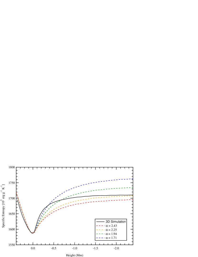
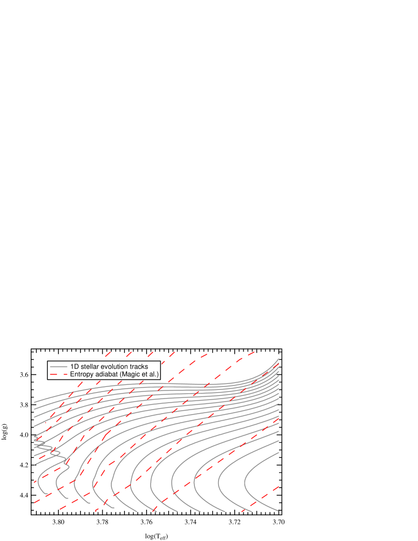
Figure 1: Top panel: Specific entropy near the surface of several 1D stellar models and one 3D RHD simulation. The models and simulation all share the same surface parameters ($\log g=4.30$, and $\log T_{\rm eff}=3.76$) and chemical composition ($Z=0.001$, $X=0.754$), but the 1D models are computed with different mixing length parameters, and so have different envelope entropy ($s_{\rm ad}$). The simulation does not contain a mixing length parameter, so the specific entropy is determined self-consistently and uniquely. Bottom panel: Contours of adiabatic entropy ($s_{\rm ad}$) in the $\log g$-$\log T_{\rm eff}$  plane, as determined by the 3D simulations of Magic et al.. The contours of $s_{\rm ad}$ (ranging from $16\cdot 10^{8}$ to $24\cdot 10^{8}$ erg $\mbox{s}^{-1}$ $\mbox{K}^{-1}$ from the lower-left to upper-right) are equivalent to contours of constant polytropic K (see e.g. Kippenhahn & Weigert 1990) and denote the convective envelope adiabats. Evolutionary tracks for a range of stellar masses ($M_{\odot}=0.75$ - $1.40$), all with the same composition parameters, and with the same constant value of the mixing length parameter $\alpha$, are shown for reference

With MLT models alone, there is no way to determine which asymptotic entropy, or adiabat, is correct. To illustrate this, in Figure 1 we show the specific entropy profiles of four 1D stellar models with identical stellar atmosphere parameters, each computed with a different value of $\alpha$. The specific entropy in both 1D models and 3D simulations was calculated with the OPAL (Rogers & Nayfonov, 2002) equation of state tables. Near the surface there exists a steep entropy gradient where radiative transfer of energy dominates, and the stratification is convectively stable. Further down, the entropy reaches a minimum and the entropy gradient switches sign, indicating that the region is convectively unstable. The entropy gradient continues to flatten with depth, with the entropy approaching a near-constant value $s_{\rm ad}$ that depends on $\alpha$, and remains roughly constant throughout the convective region until the effect of overshoot near the interior edge of the convective envelope changes the profile again.

One advantage of 3D simulations over 1D models is that simulations do not have an arbitrarily set mixing length parameter, and instead converge to a thermal structure that self-consistently links the deep adiabatic layers to the radiative atmosphere. Also shown in the upper panel of Figure 1 is the mean entropy profile for a 3D simulation with the same $\log g$ and $\log T_{\rm eff}$ as the 1D models. There are no free parameters (beyond factors for artificial viscosity and the subgrid scale model), so the resulting entropy profile is unique to the surface gravity, effective temperature and chemical composition of the simulation. Comparing the simulated entropy profile to the MLT models, we see that there is a value of $\alpha$ that can reproduce the simulated $s_{\rm ad}$. However, the complete entropy profile in the simulation cannot be matched by any of the MLT models, and this can be for a number of reasons, such as the use of an inconsistent $T$-$\tau$ relation or more likely, the absence of dynamical effects in the 1D models. We shall concentrate only on $s_{\rm ad}$ in our approach to mixing length calibration. This is similar to the recent work of Magic et al. (2015), where the entropy adiabat is related to the mixing length parameter; what we show here, is that the evolution of $s_{\rm ad}$ could potentially be described as a function of a single variable, which would be simpler to implement in 1D stellar evolution codes.

3 The entropy calibration

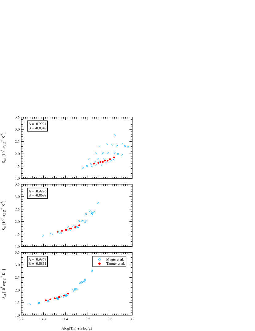
Figure 2: Adiabatic entropy ($s_{\rm ad}$) from 3D simulations of a particular chemical composition, presented along different projections of the $\log g$-$\log T_{\rm eff}$ plane. Variation in simulated entropy follows a single value functional form when presented against a particular projection that is aligned with the adiabats. The lower panel is the projection that shows the least scatter in a regression model, which is the projection that is aligned with the adiabats (i.e. the contours in the lower panel of Figure 1).

In the lower panel of Figure 1, we show contours of constant $s_{\rm ad}$ as obtained from 3D simulations by Magic et al. (2015) plotted on the $\log g$-$\log T_{\rm eff}$ plane. Also shown on the plot for reference are evolutionary tracks (computed with the Grevesse and Sauval (1998) mixture and metallicity $Z=0.018$), which are included to show the region of main-sequence stellar evolution. One striking feature of the $s_{\rm ad}$ contours is that they are nearly parallel, and for a particular chemical composition, $s_{\rm ad}$ appears to be a smooth function of $\log g$ and $\log T_{\rm eff}$. The smoothly-varying nature of the $s_{\rm ad}$ contours leads us to believe that a simple projection of the $\log g$-$\log T_{\rm eff}$ plane may sufficient to exploit the fundamental relationship between $s_{\rm ad}$, $\log g$, and $\log T_{\rm eff}$. We show that this is indeed possible in Figure 2, where simulations performed independently by Tanner et al. (2013a,b; 2014) and Magic et al. (2013) are presented on different projections of the $\log g$-$\log T_{\rm eff}$ plane. These simulations were performed with different codes and with different radiative transfer schemes, and while the simulations had similar equations of state and metallicities, they differed in their atmospheric structures: the Tanner et al. simulations assume gray atmospheres while Magic et al. do not. For all these simulations, the envelope entropy, $s_{\rm ad}$, can be projected on to a one-dimensional curve when plotted against a linear combination of $\log T_{\rm eff}$ and $\log g$  (i.e. the $\log g$-$\log T_{\rm eff}$ plane becomes $A\log T_{\rm eff}+B\log g$).

In this work, the precise values of the constants $A$ and $B$ for each metallicity were selected with a non-linear least squares minimization to a pre-determined function. First, a function of the form $(s_{\rm ad}-s_{0})=\beta\exp\left((x-x_{0})/\tau\right);x=A\log T_{\rm eff}+B\log g$ was selected by visual inspection to represent the dimensionally-reduced dataset. The choice of function is arbitrary, but the authors note that the resulting parameters $A$ and $B$ are not particularly sensitive to this, provided that the function can adequately reproduce the variation of $s_{\rm ad}$. This function function comprises six parameters that define the relationship of $s_{\rm ad}$ across the $\log g$-$\log T_{\rm eff}$ plane, and the least-squares minimization algorithm of Markwardt (2009) was then used to determine their values (listed in Table 1). The process is repeated for different convective envelope compositions (see Figure 3), each of which require a unique projection of the $\log g$-$\log T_{\rm eff}$ plane. This fitting process effectively reduces the dimensionality of the initial variation of $s_{\rm ad}$ by projecting the $\log g$-$\log T_{\rm eff}$  plane onto an axis that is aligned with the convective envelope adiabats. The process used in this work is only one possible method for reducing the dimensionality of the problem, and further study using other statistical tools, such as principle components analysis, may yield additional insights into the fundamental relationship between convection zone entropy and the stellar surface parameters.

[Fe/H]	$A$	$B$	$s_{0}$	$x_{0}$	$\beta$	$\tau$
0.5	0.9961	-0.0884	1.396	3.435	0.929	0.1009
0.0	0.9967	-0.0811	1.336	3.485	1.051	0.1056
-1.0	0.9974	-0.0720	1.304	3.540	1.127	0.0973
-2.0	0.9981	-0.0623	1.254	3.603	1.439	0.0899
-4.0	0.9985	-0.0553	1.104	3.606	1.216	0.0985

Table 1: Parameters for the function fit to $s_{\rm ad}$ from Magic et al. simulations in the projected $\log g$-$\log T_{\rm eff}$ plane ($A\log T_{\rm eff}+B\log g$).

Since the convection zone adiabatic entropy value in a stellar model is determined by the mixing length parameter, the curves in Figure 3 basically show how we need to change $\alpha$ as a function of $\log g$ and $\log T_{\rm eff}$. Of course, the first step would be to determine which numerical value of $\alpha$ yields a particular $s_{\rm ad}$  given the rest of the physics to set the mixing length scale, and thus determine how $s_{\rm ad}$ changes with $\alpha$. After setting the relationship between $s_{\rm ad}$ and $\alpha$, all that is required is to follow this relationship (i.e. the curve in Figure 3) as the star evolves. Since each time step in a stellar evolution calculation changes $\log g$ and $T_{\rm eff}$  we will need to keep changing $\alpha$ as we evolve a model.

The two panels of Figure 4 outline in principle the steps that must be taken to translate the adiabatic specific entropy derived from a 3D simulation into the corresponding entropy calibrated value of $\alpha$ to be used in the 1D MLT stellar model. Figure 4(left) shows, in the same entropy calibration plane as Figure 3, the locus of a set of 3D simulations, all with the same chemical composition, but with different values of $s_{\rm ad}$  in the deep part. Also in the left panel, are three 1D MLT models, all with the same metallicity and surface conditions as the 3D simulations. Presented relative to the projected $\log g$ and $\log T_{\rm eff}$ coordinates in this way, the evolution tracks begin on the zero-age main sequence with a relatively low $s_{\rm ad}$, which increases as the model approaches the terminal age. For the purpose of demonstrating our calibration method, we will focus only on the main-sequence phase of the evolution tracks. Because in the 1D MLT models, for a given composition, we have $s_{\rm max}=f(g,T_{\rm eff},\alpha)$, all three models were chosen, for the sake of clarity in plotting, to share the same values of $\log g$ and $\log T_{\rm eff}$, and to differ from each other only in the assumed $\alpha$.

In order to have $s_{\rm ad}$ in 1D models match that of 3D simulations, the MLT parameter $\alpha$ must be selected (and varied with evolution) so that the evolution track matches the locus of the 3D simulations. To illustrate this, we will consider a particular $\log g$ and $\log T_{\rm eff}$ represented by the vertical dashed line in the left panel of the figure. The three example main-sequence MLT models (identified on each evolution track with circles) do not match the $s_{\rm ad}$ predicted by 3D simulations, but it is clear that a value for $\alpha$ could be selected to reproduce the 3D simulated $s_{\rm ad}$ in the 1D MLT model. The intersection of the vertical line with the locus of the 3D simulations thus yields the correct entropy calibrated value of $s_{\rm ad}$ for the model with this particular $\log g$ and $\log T_{\rm eff}$. The corresponding value of $\alpha$ that will result in the desired $s_{\rm ad}$ can then be read off the plot on the right hand panel of Figure 4.

As we emphasized earlier, a mapping between the entropy calibrated $\alpha$ and $s_{\rm ad}$ will not be general. It depends sensitively on various aspects of the stellar surface conditions, some of which are imperfectly understood, and are treated differently by various researchers. The specific calibrated value of $\alpha$ is thus model dependent, as it depends on the details of the inputs used in the stellar evolution calculations. The calibration process described above cannot be carried out once (for each chemical composition) to determine a value of $\alpha$ that can applied to all other stellar models. Instead, the procedure illustrated in Fig. 4 would need to be applied as part of the stellar evolution calculation. The calibration is also particularly sensitive to the details of the $T$-$\tau$ relation. This effect is well-known in solar model construction, where, for example a larger value of $\alpha$ is needed to match the solar radius using a Krishna-Swamy model atmosphere than an Eddington approximation model atmosphere. This is an important distinction between previous attempts at mixing-length calibration, and the technique we present in this letter. For the calibration to remain generally applicable to stellar models, it must relate to the thermal structure of the convective envelope, and for the purpose of improving the accuracy of stellar radii, calibrating against $s_{\rm ad}$ is appropriate. Our method shows that the evolution of $s_{\rm ad}$ in the $\log g$ - $\log T_{\rm eff}$ plane can be presented in a convenient functional form, and we leave the final step of mapping from $s_{\rm ad}$ to $\alpha$ to the modeller.

4 Conclusion

We have provided a simple prescription of how 3D simulations can be used to calibrate the mixing length parameter in 1D stellar models. The calibration procedure based on the specific entropy adiabat presented in this paper provides a reliable way, based on simple and well established physical principles, of evaluating theoretically stellar radii of late-type stars. In this respect, the method is very general, since it depends only on the chemical composition and the well understood thermodynamic properties of deep convective stellar envelopes.

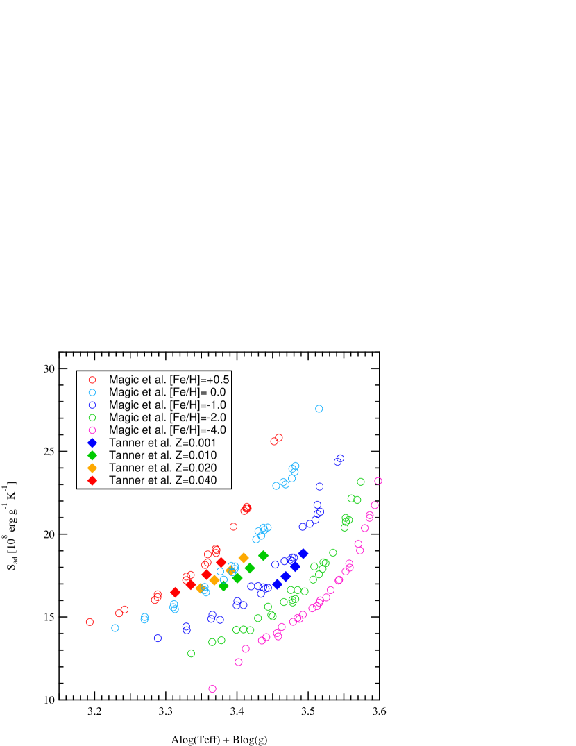
Figure 3: Adiabatic entropy from sets of 3D simulations with varied chemical compositions (similar to lowermost panel in Figure 2) presented along projections in the $\log g$-$\log T_{\rm eff}$ plane. Each metallicity requires different coefficients for $A$ and $B$, which correspond to different adiabatic contours in the $\log g$-$\log T_{\rm eff}$ plane.

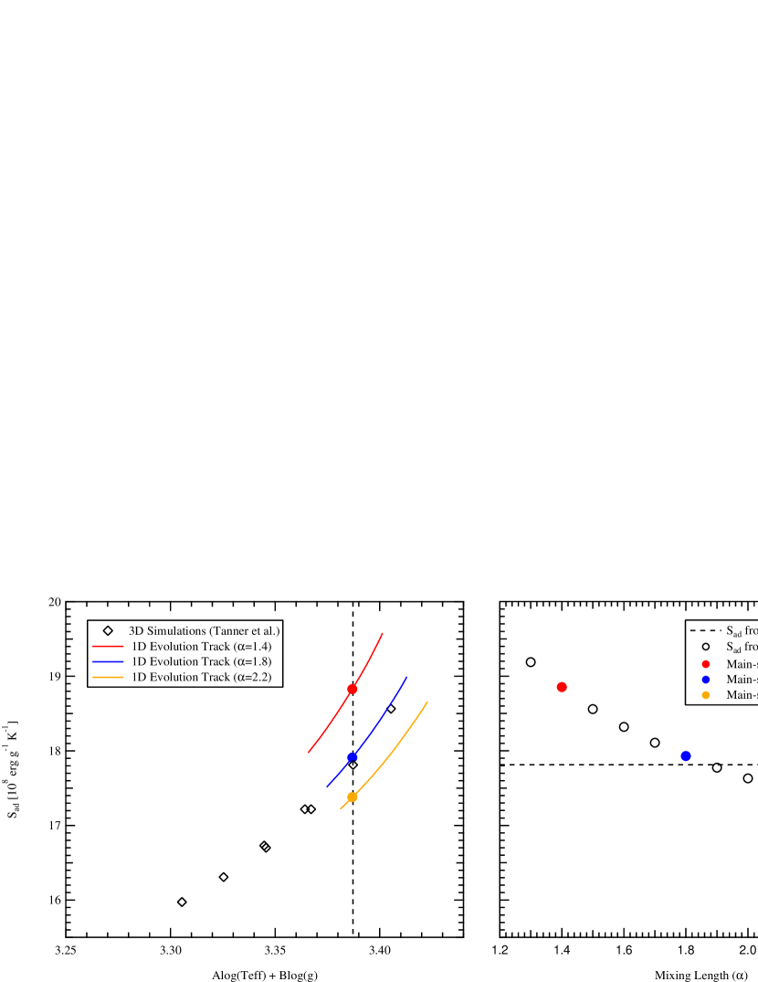
Figure 4: Stellar envelope specific entropy $s_{\rm ad}$  from 3D RHD simulations and 1D MLT stellar models. Left: Simulations and evolution tracks have the same convective envelope chemical composition, and $s_{\rm ad}$ has been plotted in a manner similar to Figure 3. The three evolution tracks are $1.1\mbox{M}_{\odot}$ models evolved to approximately $8.6\;\mbox{Gyr}$, and were constructed with different values of the mixing length parameter, $\alpha$. Right: variation of $s_{\rm ad}$ in 1D main-sequence stellar models as a function of ${\alpha}$. The stellar models have the same surface conditions, but only one value of $\alpha$ produces a stellar model matching the specific entropy from a 3D simulation (dashed line) with the same surface conditions. Note that this calibration mapping of $\alpha$ into $s_{\rm ad}$ depends on the choice of the $T$-$\tau$ relation.

References

- Arnett et al. (2010) Arnett, D. , Meakin, C., & Young, P.A. 2010, ApJ, 710, 1619
- Behara et al. (2010) Behara, N.T. , Bonifacio, P. , Ludwig, H-G., Sbordone, I., Gonzàles Hernàndez, J.I. & Caffau, E., 2010, A&A, 513, 72
- Böhm-Vitense (1958) Böhm-Vitense, E. 1958, ZAp, 46, 108
- Bonaca et al. (2012) Bonaca, A., Tanner, J.D., Basu, S. et al., 2012, ApJ, 755, 12
- Freytag & Salaris (1999) Freytag, B. & Salaris, M. 1999, ApJ, 513, 49
- Grevesse & Sauval (1998) Grevesse, N. and Sauval, A. J., 1998
- Kippenhahn & Weigert (1990) Kippenhahn, R. and Weigert, A. 1990, Stellar Structure and Evolution, Springer-Verlag, Berlin, Heidelberg & New York
- Krisnaswamy (1966) Krishna Swamy, K.S. 1966, ApJ, 145, 174
- Lebreton et al. (2001) Lebreton, Y. , Fernandes, J. & Lejeune, T. 2001, A&A, 374, 540
- Ludwig et al. (1995) Ludwig, H.-G. , Freytag, B., Steffen, M. & Wagenhuber, J. 1995, LIACo, 32, 213
- Ludwig et al. (1998) Ludwig, H-G. , Freytag, B. & Steffen, M. 1998, IAUS, 185, 115
- Ludwig et al. (1999) Ludwig, H.-G. , Freytag, B. & Steffen, M. 1999, A&A, 346, 1111
- Ludwig et al. (2009) Ludwig H.-G. , Samadi, R., Steffen, M. et al. 2009, A&A, 506, 167
- Ludwig & Kuc̆inskas (2012) Ludwig , H.-G. & Kuc̆inskas, A. 2012, A&A, 547. 118
- Markwardt (2009) Markwardt, C. B., 2009, ASPCS, 411, 251
- Magic et al. (2013) Magic, Z., Collet, R., Asplund, M. et al. 2013, A&A, 557, 26
- Magic et al. (2015) Magic, Z., Weiss, A. & Asplund, M. 2015, A&A, 573, 89
- Mihalas (1978) Mihalas, D. 1978, Stellar Atmospheres, 2nd. ed. W.H. Freeman and Company, San Francisco
- Ramírez et al. (2009) Ramírez, I., Allende Prieto, C., Koesterke, L., Lambert, D.L. & Asplund, M. 2009, A&A, 501, 1087
- Robinson et al. (2004) Robinson, F.J., Demarque,P., Li, L.H., et al. 2004, MNRAS, 347, 1208
- Robinson et al. (2005) Robinson, F.J. , Demarque, P., Guenther, D.B., Kim, Y.-C. & Chan, K.L. 2005, MNRAS, 362, 1031
- Rogers & Nayfonov (2002) Rogers, F. J. and Nayfonov, A., 2002
- Straka et al. (2006) Straka, C.W., Demarque, P., Guenther, D.B., Li. L. & Robinson, F.J. 2006, ApJ, 636, 1078
- Straka et al. (2007) Straka, C.W., Demarque, P. & Robinson, F.J. 2007, IAUS, 239, 388
- Tanner et al. (2013a) Tanner, J.D., Basu, S. & Demarque, P. 2013a, ApJ, 767, 78
- Tanner et al. (2013b) Tanner, J.D., Basu, S. & Demarque, P. 2013b, ApJ, 778, 117
- Tanner (2014a) Tanner, J.D. 2014a, Chapter 7, PhD Thesis, Yale University
- Tanner (2014b) Tanner, J.D., Basu, S. & Demarque, P. 2014b, ApJ, 785, 13
- Trampedach & Stein (2011) Trampedach, R. & Stein,R.F. 2011, ApJ, 731, 78
- Trampedach et al. (2013) Trampedach, R., Asplund, M., Collet, R., Nordlund, Å. & Stein, R. F. 2013, ApJ, 769, 18
- Trampedach et al. (2014a) Trampedach, R. , Stein, R.F., Christensen-Dalsgaard, J., Nordlund,Å. & Asplund, M. 2014a, MNRAS, 442, 805
- Trampedach et al. (2014b) Trampedach, R. , Stein, R.F., Christensen-Dalsgaard, J., Nordlund,Å. & Asplund, M. 2014b, MNRAS, 445, 4366
- Vernazza et al. (1981) Vernazza, J.E., Avrett, E.H. & Loeser, R. 1981, ApJ, 45, 635
- Yıldız et al. (2006) Yıldız, M., Yakut, K., Bakiş, H. & Noels, A. 2006, MNRAS, 368, 1941