Towards Real-time Simulation of Hyperelastic Materials

Abstract

We present a new method for real-time physics-based simulation supporting many different types of hyperelastic materials. Previous methods such as Position Based or Projective Dynamics are fast, but support only limited selection of materials; even classical materials such as the Neo-Hookean elasticity are not supported. Recently, Xu et al. [2015] introduced new “spline-based materials” which can be easily controlled by artists to achieve desired animation effects. Simulation of these types of materials currently relies on Newton’s method, which is slow, even with only one iteration per timestep. In this paper, we show that Projective Dynamics can be interpreted as a quasi-Newton method. This insight enables very efficient simulation of a large class of hyperelastic materials, including the Neo-Hookean, spline-based materials, and others. The quasi-Newton interpretation also allows us to leverage ideas from numerical optimization. In particular, we show that our solver can be further accelerated using L-BFGS updates (Limited-memory Broyden-Fletcher-Goldfarb-Shanno algorithm). Our final method is typically more than 10 times faster than one iteration of Newton’s method without compromising quality. In fact, our result is often more accurate than the result obtained with one iteration of Newton’s method. Our method is also easier to implement, implying reduced software development costs.

1 Introduction

Physics-based animation is an important tool in computer graphics even though creating visually compelling simulations often requires a lot of patience. Waiting for results is not an option in real-time simulations, which are necessary in applications such as computer games and training simulators, e.g., surgery simulators. Previous methods for real-time physics such as Position Based Dynamics [Müller et al. 2007] or Projective Dynamics [Bouaziz et al. 2014] have been successfully used in many applications and commercial products, despite the fact that these methods support only a restricted set of material models. Even classical models from continuum mechanics, such as the Neo-Hookean, St. Venant-Kirchoff, or Mooney-Rivlin materials, are not supported by Projective Dynamics. We tried to emulate their behavior with Projective Dynamics, but despite our best efforts, there are still obvious visual differences when compared to simulations with the original non-linear materials.

The advantages of more general material models were nicely demonstrated in the recent work of Xu et al. xu2015nonlinear, who proposed a new class of spline-based materials particularly suitable for physics-based animation. Their user-friendly spline interface enables artists to easily modify material properties in order to achieve desired animation effects. However, their system relies on Newton’s method, which is slow, even if the number of Newton’s iterations per frame is limited to one. Our method enables fast simulation of spline-based materials, combining the benefits of artist-friendly material interfaces with the advantages of fast simulation, such as rapid iterations and/or higher resolutions.

Physics-based simulation can be formulated as an optimization problem where we minimize a multi-variate function $g$. Newton’s method minimizes $g$ by performing descent along direction $-(\nabla^{2}g)^{-1}\nabla g$, where $\nabla^{2}g$ is the Hessian matrix, and $\nabla g$ is the gradient. One problem of Newton’s method is that the Hessian $\nabla^{2}g$ can be indefinite, in which case the Newton’s direction could erroneously increase $g$. This undesired behavior can be prevented by so-called “definiteness fixes” [Teran et al. 2005, Nocedal and Wright 2006]. While definiteness fixes require some computational overheads, the slow speed of Newton’s method is mainly caused by the fact that the Hessian changes at every iteration, i.e., we need to solve a new linear system for every Newton step.

The point of departure for our method is the insight that Projective Dynamics can be interpreted as a special type of quasi-Newton method. In general, quasi-Newton methods [Nocedal and Wright 2006] work by replacing the Hessian $\nabla^{2}g$ with a linear operator $\mathbf{A}$, where $\mathbf{A}$ is positive definite and solving linear systems $\mathbf{A}\mathbf{x}=\mathbf{b}$ is fast. The descent directions are then computed as $-\mathbf{A}^{-1}\nabla g$ (where the inverse is of course not explicitly evaluated, in fact, $\mathbf{A}$ is often not even represented with a matrix). The trade-off is that if $\mathbf{A}$ is a poor approximation of the Hessian, the quasi-Newton method may converge slowly. Unfortunately, coming up with an effective approximation of the Hessian is not easy. We tried many previous quasi-Newton methods, but even after boosting their performance with L-BFGS [Nocedal and Wright 2006], we were unable to obtain an effective method for real-time physics. We show that Projective Dynamics can be re-formulated as a quasi-Newton method with some remarkable properties, in particular, the resulting $\mathbf{A}_{\mathtt{our}}$ matrix is constant and positive definite. This re-formulation enables us to generalize the method to hyperelastic materials not supported by Projective Dynamics, such as the Neo-Hookean or spline-based materials. Even though the resulting solver is slightly more complicated than Projective Dynamics (in particular, we must employ a line search to ensure stability), the computational overhead required to support more general materials is rather small.

The quasi-Newton formulation also allows us to further improve convergence of our solver. We propose using L-BFGS, which uses curvature information estimated from a certain number of previous iterates to improve the accuracy of our Hessian approximation $\mathbf{A}_{\mathtt{our}}$. Adding the L-BFGS Hessian updates introduces only a small computational overhead while accelerating the convergence of our method. However, this is not a silver bullet, because the performance of L-BFGS highly depends on the quality of the initial Hessian approximation. With previous quasi-Newton methods, we observed rather disappointing convergence properties (see Figure 6). However, the combination of our Hessian approximation $\mathbf{A}_{\mathtt{our}}$ with L-BFGS is quite effective and can be interpreted as a generalization of the recently proposed Chebyshev Semi-Iterative method for accelerating Projective Dynamics [Wang 2015].

The L-BFGS convergence boosting is compatible with our first contribution, i.e., fast simulation of complex non-linear materials. Specifically, we can simulate any materials satisfying the Valanis-Landel assumption [Valanis and Landel 1967] which includes many classical materials, such as St. Venant-Kirchhoff, Neo-Hookean, Mooney-Rivlin, and also the recently proposed spline-based materials [Xu et al. 2015] (none of which is supported by Projective Dynamics). In summary, our final method achieves faster convergence than Projective Dynamics while being able to simulate a large variety of hyperelastic materials.

2 Related Work

The work of Terzopoulos et al. terzopoulos1987elastically pioneered physics-based animation, nowadays an indispensable tool in feature animation and visual effects. Real-time physics became widespread only more recently, with first success stories represented by real-time rigid body simulators, commercially offered by companies such as Havok since early 2000s. Fast simulation of deformable objects is more challenging because they feature many more degrees of freedom than rigid bodies. Fast simulations of deformable objects using shape matching [Müller et al. 2005, Rivers and James 2007] paved the way towards more general Position Based Dynamics methods [Müller et al. 2007, Stam 2009]. The past decade witnessed rapid development of Position Based methods, including improvements of the convergence [Müller 2008, Kim et al. 2012], robust simulation of elastic models [Müller and Chentanez 2011], generalization to fluids [Macklin and Müller 2013] and continuum-based materials [Müller et al. 2014, Bender et al. 2014a], unified solvers including multiple phases of matter [Macklin et al. 2014], and most recently, methods to avoid element inversion [Müller et al. 2015]. We refer to a recent survey [Bender et al. 2014b] for a more detailed summary of Position Based methods.

A new interpretation of Position Based methods was offered by Liu et al. liu2013fast, observing that Position Based Dynamics can be interpreted as an approximate solver for Implicit Euler time-stepping. The same paper introduces a fast local/global solver for mass-spring systems integrated using Implicit Euler. This method was later generalized to Projective Dynamics [Bouaziz et al. 2014] by combining the ideas of [Liu et al. 2013] with a shape editing system “Shape-Up” [Bouaziz et al. 2012]. Recently, a Chebyshev Semi-Iterative method [Wang 2015] has been proposed to accelerate convergence of Projective Dynamics, while exploring also highly parallel GPU implementations of real-time physics.

Multi-grid methods represent another approach to accelerate physics-based simulations [Georgii and Westermann 2006, Müller 2008, Wang et al. 2010, McAdams et al. 2011, Tamstorf et al. 2015]. Multi-grid methods are attractive especially for highly detailed meshes where sparse direct solvers become hindered by high memory requirements. However, constructing multi-resolution data structures and picking suitable parameters is not a trivial task. Another way to speed up FEM is by using subspace simulation where the nodal degrees of freedom are replaced with a low-dimensional linear subspace [Barbič and James 2005, An et al. 2008, Li et al. 2014]. These methods can be very efficient; however, deformations that were not accounted for during the subspace construction may not be well represented. A variety of approaches have been designed to address this limitation while trying to preserve efficiency [Harmon and Zorin 2013, Teng et al. 2014, Teng et al. 2015]. Simulating at coarser resolutions is also possible, while crafting special data-driven materials which avoid the loss of accuracy typically associated with lower resolutions [Chen et al. 2015].

The concept of constraint projection, which appears in both Position Based and Projective Dynamics, is also central to the Fast Projection method [Goldenthal et al. 2007] and strain-limiting techniques [Thomaszewski et al. 2009, Narain et al. 2012]. The Fast Projection method and Position Based Dynamics formulate physics simulation as a constrained optimization problem that is solved by linearizing the constraints in the spirit of sequential quadratic programming [Macklin et al. 2014]. The resulting Karush-Kuhn-Tucker (KKT) equation system is then solved using a direct solver [Goldenthal et al. 2007] or an iterative method such as Gauss-Seidel [Müller et al. 2007, Stam 2009, Fratarcangeli and Pellacini 2015], Jacobi [Macklin and Müller 2013], or their under/over-relaxation counterparts [Macklin et al. 2014]. By using a constrained optimization formulation the Fast Projection method and Position Based Dynamics are designed for solving infinitely stiff systems but are not appropriate to handle soft materials. This problem can be overcome by regularizing the KKT system [Servin et al. 2006, Tournier et al. 2015], leading to approaches that can accurately handle extremely high tensile forces (e.g., string of a bow) but also support soft (compliant) constraints. However, these methods are slower than Projective Dynamics because a new linear system has to be solved at each iteration.

The idea of quasi-Newton methods in elasticity is not new and has been studied long time before real-time simulations were feasible. Several research papers have been done to accelerate Newton’s method in FEM simulations by updating the Hessian approximation only once every frame [Bathe and Cimento 1980, Fish et al. 1995]. However, even one Hessian update is usually so computationally expensive that can not fit into the computing time limit of real-time applications. Deuflhard deuflhard2011newton minimizes the number of Hessian factorizations by carefully scheduled Hessian updates. But the update rate will heavily depend on the deformation. A good Hessian approximation suitable for realtime applications should be easy to refactorize or capable of prefactorization. One straightforward constant approximation which is good for prefactorization is the Hessian evaluated at the rest-pose (undeformed configuration). The rest-pose is positive semi-definite and its use at any configuration enables pre-factorization. Unfortunately, the actual Hessian of deformed configurations is often very different from the rest-pose Hessian and this approximation is therefore not satisfactory for larger deformations [Müller et al. 2002].

To improve upon this, Müller et al. Muller2002vertexwarp introduced per-vertex “stiffness warping” of the rest-pose Hessian, which is more accurate and can still leverage pre-factorized rest-pose Hessian. Unfortunately, the per-vertex stiffness warping approach can introduce non-physical ghost forces which violate momentum conservation and can lead to instabilities [Müller and Gross 2004]. This problem was addressed by per-element stiffness warping [Müller and Gross 2004] which avoids the ghost forces but, unfortunately, the per-element-warped stiffness matrices need to be re-factorized, introducing computational overheads which are prohibitive in real-time simulation. For corotated elasticity, Hecht et al. Hecht:2012:USC proposed an improved method which can re-use previously computed Hessian factorization. Specifically, the sparse Cholesky factors are updated only when necessary and also only where necessary. This spatio-temporal staging of Cholesky updates improves run-time performance, however, the Cholesky updates are still costly and their scheduling can be problematic especially in real-time applications, which require approximately constant per-frame computing costs. Also, the frequency of Cholesky updates depends on the simulation: fast motion with large deformations will require more frequent updates and thus more computation, or risking ghost forces and potential instabilities. Neither is an option in real-time simulators.

Our re-formulation of Projective Dynamics as a quasi-Newton method reveals relationships to so called “Sobolev gradient methods”, which have been studied since the 1980s in the continuous setting [Neuberger 1983]; see also the more recent monograph [Neuberger 2009]. The idea of quasi-Newton methods appears already in [Desbrun et al. 1999, Hauth and Etzmuss 2001] in the context of mass-spring systems and, more recently, in [Martin et al. 2013] in the context of geometry processing. Martin et al. martin2013efficient also propose multi-scale extensions and discuss an application in physics-based simulation, but consider only the case of thin shells and their numerical method alters the physics of the simulated system. Quasi-Newton methods are also useful in situations where computation of the Hessian would be expensive or impractical [Nocedal and Wright 2006]. In character animation, Hahn et al. Hahn2012 used BFGS to simulate physics in “Rig Space”, which is challenging because the rig is a black box function and its derivatives are approximated using finite differences.

3 Background

Projective Dynamics. We start by introducing our notation and recapitulating the key concepts of Projective Dynamics. Let $\mathbf{x}\in\mathbb{R}^{n\times 3}$ be the current (deformed) state of our system containing $n$ nodes, each with three spatial dimensions. Projective Dynamics requires a special form of elastic potential energies, based on the concept of constraint projection. Specifically, Projective Dynamics energy for element number $i$ is defined as:

$$E_{i}(\mathbf{x})=\min_{\mathbf{p}_{i}\in{\cal{M}}_{i}}\tilde{E}_{i}(\mathbf{x},\mathbf{p}_{i}),\ \ \tilde{E}_{i}(\mathbf{x},\mathbf{z})=\|\mathbf{G}_{i}\mathbf{x}-\mathbf{z}\|^{2}_{F}$$ (1)

where $\|\cdot\|_{F}$ is the Frobenius norm, ${\cal{M}}_{i}$ is a constraint manifold, $\mathbf{p}_{i}$ is an auxiliary “projection variable”, and $\mathbf{G}_{i}$ is a discrete differential operator represented, e.g., by a sparse matrix. For example, if element number $i$ is a tetrahedron, ${\cal{M}}_{i}$ is $SO(3)$, and $\mathbf{G}_{i}$ is deformation gradient operator [Sifakis and Barbič 2012], we obtain the well-known as-rigid-as-possible material model [Chao et al. 2010]. Another elementary example is a spring, where the element is an edge, ${\cal{M}}_{i}$ is a sphere, and $\mathbf{G}_{i}$ subtracts two endpoints of the spring. If all elements are springs, Projective Dynamics becomes equivalent to the work of Liu et al. liu2013fast. The key property of $\mathbf{G}_{i}$ is that constant vectors are in its nullspace, which makes $E_{i}$ translation invariant. The total energy of the system is:

$$E(\mathbf{x})=\sum_{i}w_{i}E_{i}(\mathbf{x})$$ (2)

where $i$ indexes elements and $w_{i}>0$ is a positive weight, typically defined as the product of undeformed volume and stiffness.

Time integration. As discussed by Martin et al. martin2011example, Backward Euler time integration can be expressed as a minimization of:

$$g(\mathbf{x})=\frac{1}{2h^{2}}\underbrace{\mathop{\text{tr}}((\mathbf{x}-\mathbf{y})^{\mathsf{T}}\mathbf{M}(\mathbf{x}-\mathbf{y}))}_{\mathrm{inertia}}+\ \!\!\!\!\underbrace{E(\mathbf{x})}_{\mathrm{elasticity}}$$ (3)

where $\mathbf{y}$ is a constant depending only on previously computed states, $\mathbf{M}$ is a positive definite mass matrix (typically diagonal – mass lumping), and $h>0$ is the time step (we use fixed $h$ corresponding to the frame rate of $30fps$, i.e., $h=1/30s$). The trace ($\mathop{\text{tr}}$) reflects the fact that there are no dependencies between the $x,y,z$ coordinates, which enables us to work only with $n\times n$ matrices (as opposed to more general $3n\times 3n$ matrices). This is somewhat moot in the context of the mass matrix $\mathbf{M}$, but it will be more important in the following. The constant $\mathbf{y}$ is defined as $\mathbf{y}:=2\mathbf{q}_{l}-\mathbf{q}_{l-1}+h^{2}\mathbf{M}^{-1}\mathbf{f}_{\text{ext}}$, where $\mathbf{q}_{l}\in\mathbb{R}^{n\times 3}$ is the current state, $\mathbf{q}_{l-1}$ the previous state, and $\mathbf{f}_{\text{ext}}\in\mathbb{R}^{n\times 3}$ are external forces such as gravity. The minimizer of $g(\mathbf{x})$ will become the next state, $\mathbf{q}_{l+1}$. Intuitively, the first term in Eq. 3 can be interpreted as “inertial potential,” attracting $\mathbf{x}$ towards $\mathbf{y}$, where $\mathbf{y}$ corresponds to state predicted by Newton’s first law – motion without the presence of any internal forces. The second term penalizes states $\mathbf{x}$ with large elastic deformations. Minimization of $g(\mathbf{x})$ corresponds to finding balance between the two terms. Note that many other implicit integration schemes can also be expressed as minimization problems similar to Eq. 3. In particular, we have implemented Implicit Midpoint, which has the desirable feature of being symplectic [Hairer et al. 2002, Kharevych et al. 2006]. Unfortunately, in our experiments we found Implicit Midpoint to be markedly less stable than Backward Euler and, therefore, we continue to use Backward Euler despite its numerical damping.

Local/global solver. The key idea of Projective Dynamics is to expose the auxiliary projection variables $\mathbf{p}_{i}$, taking advantage of the special energy form according to Eq. 1. To simplify notation, we stack all projection variables into $\mathbf{p}\in\mathbb{R}^{c\times 3}$ and define binary selector matrices $\mathbf{S}_{i}$ such that $\mathbf{p}_{i}=\mathbf{S}_{i}\mathbf{p}$. Projective Dynamics uses the augmented objective:

$$\tilde{g}(\mathbf{x},\mathbf{p})=\frac{1}{2h^{2}}{\mathop{\text{tr}}((\mathbf{x}-\mathbf{y})^{\mathsf{T}}\mathbf{\mathbf{M}}(\mathbf{x}-\mathbf{y}))}+\sum_{i}w_{i}\tilde{E}(\mathbf{x},\mathbf{S}_{i}\mathbf{p})$$ (4)

which is minimized over both $\mathbf{x}$ and $\mathbf{p}$, subject to the constraint $\mathbf{p}\in{\cal{M}}$, where ${\cal{M}}$ is a cartesian product of the individual constraint manifolds. The optimization is solved using an alternating (local/global) solver. In the local step, $\mathbf{x}$ is assumed to be fixed; the optimal $\mathbf{p}$ are given by projections on individual constraint manifolds, e.g., projecting each deformation gradient (a $3\times 3$ matrix) on $SO(3)$. In the global step, $\mathbf{p}$ is assumed to be fixed and we rewrite the objective $\tilde{g}(\mathbf{x},\mathbf{p})$ in matrix form:

$$\frac{1}{2h^{2}}{\mathop{\text{tr}}((\mathbf{x}-\mathbf{y})^{\mathsf{T}}\mathbf{\mathbf{M}}(\mathbf{x}-\mathbf{y}))}+\frac{1}{2}\mathop{\text{tr}}(\mathbf{x}^{\mathsf{T}}\mathbf{L}\mathbf{x})-\mathop{\text{tr}}(\mathbf{x}^{\mathsf{T}}\mathbf{J}\mathbf{p})+C$$ (5)

where $\mathbf{L}:=\sum w_{i}\mathbf{G}_{i}^{\mathsf{T}}\mathbf{G}_{i}$, $\mathbf{J}:=\sum w_{i}\mathbf{G}_{i}^{\mathsf{T}}\mathbf{S}_{i}$, and the constant $C$ is irrelevant for optimization. For a fixed $\mathbf{p}$, the minimization of $\tilde{g}(\mathbf{x},\mathbf{p})$ can be accomplished by finding $\mathbf{x}$ with a vanishing gradient, i.e., $\nabla_{\mathbf{x}}\tilde{g}(\mathbf{x},\mathbf{p})=0$. Computing the gradient yields some convenient simplifications (the traces disappear):

$$\nabla_{\mathbf{x}}\tilde{g}(\mathbf{x},\mathbf{p})=\frac{1}{h^{2}}\mathbf{M}(\mathbf{x}-\mathbf{y})+\mathbf{L}\mathbf{x}-\mathbf{J}\mathbf{p}$$ (6)

Equating the gradient to zero leads to the solution:

$$\mathbf{x}^{*}=(\mathbf{M}/h^{2}+\mathbf{L})^{-1}(\mathbf{J}\mathbf{p}+\mathbf{M}\mathbf{y}/h^{2})$$ (7)

The matrix $\mathbf{M}/h^{2}+\mathbf{L}$ is symmetric positive definite and therefore $\mathbf{x}^{*}$ is a global minimum (for fixed $\mathbf{p}$). The key computational advantage of Projective Dynamics is that $\mathbf{M}/h^{2}+\mathbf{L}$ does not depend on $\mathbf{x}$, which allows us to pre-compute and repeatedly reuse its sparse Cholesky factorization to quickly solve for $\mathbf{x}^{*}$, which is the result after one local and global step. The local and global steps are repeated for a fixed number of iterations (typically 10 or 20).

4 Method

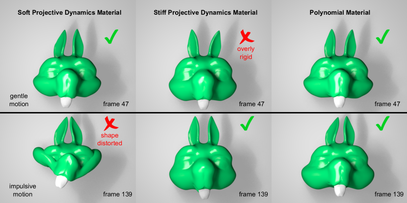
Figure 1: Animating jiggly squirrel head. The squirrel head is driven by a gentle keyframed motion in the top row, and by a faster, impulsive motion in the bottom row. Soft Projective Dynamics material (left column) creates nice secondary motion, but does not prevent large distortions of the shape. If we stiffen the Projective Dynamics material (middle column), we prevent the distortions, but also kill the secondary motion. Our polynomial material $a(x)=\mu(x-1)^{4},b(x)=0,c(x)=0$ (right column) achieves the desired effect of jiggling without large shape distortions.

As described in the previous section, Projective Dynamics relies on the special type of elastic energies according to Eq. 1. Let us now describe how Projective Dynamics can be interpreted as a quasi-Newton method. The first step is to compute the gradient of the objective $g(\mathbf{x})$ from Eq. 3. The energy $E(\mathbf{x})$ used in this objective contains constrained minimization over the projection variables $\mathbf{p}_{i}\in{\cal{M}}_{i}$ (see Eq. 1 and Eq. 2). Equivalently, we can interpret the $\mathbf{p}_{i}$ as functions of $\mathbf{x}$ realizing the projections, according to Eq. 1. Nevertheless, the gradient $\nabla g(\mathbf{x})$ can still be computed easily – in fact, it is exactly equivalent to $\nabla_{\mathbf{x}}\tilde{g}(\mathbf{x},\mathbf{p})$ from Eq. 6 where we assumed that $\mathbf{p}$ is constant. This at first surprising fact has been observed in previous work [Chao et al. 2010, Bouaziz et al. 2012]. Intuitively, the reason is that if we infinitesimally perturb $\mathbf{x}$, its projection $\mathbf{p}_{i}(\mathbf{x})$ can move only in the tangent space of ${\cal{M}}_{i}$ and therefore, the differential $\delta\mathbf{p}_{i}(\mathbf{x})$ has no effect on $\delta\|\mathbf{x}-\mathbf{p}_{i}(\mathbf{x})\|^{2}$. As an intuitive explanation, imagine that $\mathbf{x}$ is a space shuttle projected to its closest point on Earth $\mathbf{p}_{i}(\mathbf{x})$; to first order, the distance of the space shuttle from Earth does not depend on the tangent motion $\delta\mathbf{p}_{i}(\mathbf{x})$. Please see the Appendix for a more formal discussion. In summary, the gradient of Eq. 3 is:

$$\nabla{g}(\mathbf{x})=\frac{1}{h^{2}}\mathbf{M}(\mathbf{x}-\mathbf{y})+\mathbf{L}\mathbf{x}-\mathbf{J}\mathbf{p}(\mathbf{x})$$ (8)

where $\mathbf{p}(\mathbf{x})$ is a function stacking all of the individual projections $\mathbf{p}_{i}(\mathbf{x})$. Newton’s method would proceed by computing second derivatives, i.e, the Hessian matrix $\nabla^{2}g(\mathbf{x})$, and use it to compute a descent direction $-(\nabla^{2}g(\mathbf{x}))^{-1}\nabla g(\mathbf{x})$. Note that definiteness fixes may be necessary to guarantee this will really be a descent direction [Gast et al. 2015].

What happens if we modify Newton’s method by using $\mathbf{M}/h^{2}+\mathbf{L}$ instead of the Hessian $\nabla^{2}g(\mathbf{x})$? Simple algebra reveals:

$$(\mathbf{M}/h^{2}+\mathbf{L})^{-1}\nabla{g}(\mathbf{x})=\mathbf{x}-(\mathbf{M}/h^{2}+\mathbf{L})^{-1}(\mathbf{J}\mathbf{p}(\mathbf{x})+\mathbf{M}\mathbf{y}/h^{2})$$

However, the latter term is equivalent to the result of one iteration of the local/global steps of Projective Dynamics, see Eq. 7. Therefore, $(\mathbf{M}/h^{2}+\mathbf{L})^{-1}\nabla{g}(\mathbf{x})=\mathbf{x}-\mathbf{x}^{*}$ and we can interpret $\mathbf{d}_{\mathrm{PD}}:=-(\mathbf{M}/h^{2}+\mathbf{L})^{-1}\nabla{g}(\mathbf{x})$ as a descent direction (this time there is no need for any definiteness fixes). Projective Dynamics can be therefore understood as a quasi-Newton method which computes the next iterate as $\mathbf{x}+\mathbf{d}_{\mathrm{PD}}$. Typically, quasi-Newton methods use line search techniques [Nocedal and Wright 2006] to find parameter $\alpha>0$ such that $\mathbf{x}+\alpha\mathbf{d}_{\mathrm{PD}}$ reduces the objective as much as possible. However, with Projective Dynamics energies according to Eq. 1, the optimal value is always $\alpha=1$.

4.1 More general materials

The interpretation of Projective Dynamics as a quasi-Newton method suggests that a similar optimization strategy might be effective for more general elastic potential energies. First, let us focus on isotropic materials, deferring the discussion of anisotropy to Section 4.4. The assumption of isotropy (material-space rotation invariance) together with world-space rotation invariance means that we can express elastic energy density function $\Psi$ as a function of singular values of the deformation gradient [Irving et al. 2004, Sifakis and Barbič 2012]. In the volumetric case, we have three singular values $\sigma_{1},\sigma_{2},\sigma_{3}\in\mathbb{R}$, also known as “principal stretches”. The function $\Psi(\sigma_{1},\sigma_{2},\sigma_{3})$ must be invariant to any permutation of the principal stretches, e.g., $\Psi(\sigma_{1},\sigma_{2},\sigma_{3})=\Psi(\sigma_{2},\sigma_{1},\sigma_{3})$ etc. Because directly working with such functions $\Psi$ could be cumbersome, we instead use the Valanis-Landel hypothesis [Valanis and Landel 1967], which assumes that:

$$\begin{split}\Psi(\sigma_{1},\sigma_{2},\sigma_{3})=a(\sigma_{1})+a(\sigma_{2})+a(\sigma_{3})+\\ b(\sigma_{1}\sigma_{2})+b(\sigma_{2}\sigma_{3})+b(\sigma_{1}\sigma_{3})+c(\sigma_{1}\sigma_{2}\sigma_{3})\end{split}$$ (9)

where $a,b,c:\mathbb{R}\rightarrow\mathbb{R}$. Many material models can be written in the Valanis-Landel form, including linear corotated material [Sifakis and Barbič 2012], St. Venant-Kirchhoff, Neo-Hookean, and Mooney-Rivlin. The recently proposed spline-based materials [Xu et al. 2015] are also based on the Valanis-Landel assumption. How can we generalize Projective Dynamics to these types of materials? Invoking the quasi-Newton interpretation discussed above, our method will minimize the objective $g$ by performing descent along direction $\mathbf{d}(\mathbf{x}):=-(\mathbf{M}/h^{2}+\mathbf{L})^{-1}\nabla{g}(\mathbf{x})$. The mass matrix $\mathbf{M}$ and step size $h$ are defined as before, and computing $\nabla{g}(\mathbf{x})$ is straightforward. But how to define a matrix $\mathbf{L}$ for a given material model? This matrix can still have the form $\mathbf{L}:=\sum w_{i}\mathbf{G}_{i}^{\mathsf{T}}\mathbf{G}_{i}$, but the question is how to choose the weights $w_{i}$. In Projective Dynamics, we assumed the weights are given as $w_{i}=V_{i}k_{i}$, where $V_{i}>0$ is rest-pose volume of $i$-th element, and $k_{i}>0$ is a stiffness parameter provided by the user. In our case, the user instead specifies a material model according to Eq. 9 from which we have to infer the appropriate $k_{i}$ value. In the following we drop the subscript $i$ for ease of notation.

For linear materials (Hooke’s law), stiffness is given as the second derivative of elastic energy. Therefore, it would be tempting to set $k$ equal to the second derivative of $\Psi$ at the rest pose (corresponding to $\sigma_{1}=\sigma_{2}=\sigma_{3}=1$), which evaluates to $a^{\prime\prime}(1)+2b^{\prime\prime}(1)+c^{\prime\prime}(1)$, regardless of whether we differentiate with respect to $\sigma_{1}$, $\sigma_{2}$, or $\sigma_{3}$. Even though this method would produce suitable $k$ for some materials (such as corotated elasticity), it does not work e.g. for a polynomial material defined as $a(x)=\mu(x-1)^{4},b(x)=0,c(x)=0$. Already this relatively simple material can facilitate certain animation tasks, such as creating a cartoon squirrel head which jiggles, but does not overly distort its shape, see Figure 1. However, with this material, the second derivatives at $x=1$ evaluates to zero regardless of the value of $\mu$, which would lead to zero stiffness which is obviously not a good approximation. The problem is the second derivative takes into account only infinitesimally small neighborhood of $x=1$, i.e., the rest pose. However, we need a single value of $k$ which will work well in the entire range of deformations expected in our simulations. To capture this requirement, we define an interval $[x_{\mathrm{start}},x_{\mathrm{end}}]$ where we expect our principal stretches to be. We consider the following stress function:

$$\begin{split}\left.\frac{\partial\Psi}{\partial\sigma_{1}}\right|_{\sigma_{2}=1,\sigma_{3}=1}=a^{\prime}(\sigma_{1})+2b^{\prime}(\sigma_{1})+c^{\prime}(\sigma_{1})\end{split}$$ (10)

and define our $k$ as the slope of the best linear approximation of Eq. 10 for $\sigma_{1}\in[x_{\mathrm{start}},x_{\mathrm{end}}]$. Note that due to the symmetry of the Valanis-Landel assumption, we would obtain exactly the same result if we differentiated with respect to $\sigma_{2}$ or $\sigma_{3}$ (instead of $\sigma_{1}$ as above). We study different choices of $[x_{\mathrm{start}},x_{\mathrm{end}}]$ intervals in Section 5. In summary, the results are not very sensitive on the particular choice of $x_{\mathrm{start}}$ and $x_{\mathrm{end}}$. The key fact is that regardless of the specific setting of $x_{\mathrm{start}}$ and $x_{\mathrm{end}}$, spatial variations of $\mu$ are correctly taken into account, i.e., softer and stiffer parts of the simulated object will have different $\mu$ coefficients (e.g., in our squirrel head we made the teeth more stiff). Even though all elements have the same $[x_{\mathrm{start}},x_{\mathrm{end}}]$ interval, the resulting matrices $\mathbf{L}$ and $\mathbf{J}$ properly reflect the spatially varying stiffness.

1 $\mathbf{x}_{1}:=\mathbf{y}$; $g(\mathbf{x}_{1}):=\mathtt{evalObjective}(\mathbf{x}_{1})$

2 for $k=1,\dots,\mathrm{numIterations}$ do

3       $\nabla g(\mathbf{x}_{k}):=\mathtt{evalGradient}(\mathbf{x}_{k})$

4       $\mathbf{d}(\mathbf{x}_{k}):=-(\mathbf{M}/h^{2}+\mathbf{L})^{-1}\nabla{g}(\mathbf{x}_{k})$

5       $\alpha:=2$

6       repeat

7             $\alpha:=\alpha/2$

8             $\mathbf{x}_{k+1}:=\mathbf{x}_{k}+\alpha\mathbf{d}(\mathbf{x}_{k})$

9             $g(\mathbf{x}_{k+1}):=\mathtt{evalObjective}(\mathbf{x}_{k+1})$

10            

11      until $g(\mathbf{x}_{k+1})\leq g(\mathbf{x}_{k})+\gamma\alpha\ \mathrm{tr}((\nabla g(\mathbf{x}_{k}))^{\mathsf{T}}\mathbf{d}(\mathbf{x}_{k}))$;

12 end for

Algorithm 1 Quasi-Newton Solver

Line search. With Projective Dynamics materials (Eq. 1), the line search parameter $\alpha=1$ is always guaranteed to decrease the objective $g$ (Eq. 3). Unfortunately, this is no longer true in our generalized quasi-Newton setting, where it is easy to find examples where $g(\mathbf{x}+\mathbf{d}(\mathbf{x}))>g(\mathbf{x})$, i.e., taking a step of size one actually increases the objective. This can lead to erroneous energy accumulation, potentially resulting in catastrophic failure of the simulation (“explosions”), as shown in Figure 2. Fortunately, thanks to the fact that $\mathbf{M}/h^{2}+\mathbf{L}$ is positive definite, $\mathbf{d}(\mathbf{x})$ is guaranteed to be a descent direction. Therefore, there exists $\alpha>0$ such that $g(\mathbf{x}+\alpha\mathbf{d}(\mathbf{x}))\leq g(\mathbf{x})$ (unless we are already at a critical point $\nabla g(\mathbf{x})=\mathbf{0}$, at which point the optimization is finished). In fact, we can ask for even more, i.e., we can always find $\alpha>0$ such that $g(\mathbf{x}+\alpha\mathbf{d}(\mathbf{x}))\leq g(\mathbf{x})+\gamma\alpha\mathop{\text{tr}}((\nabla g(\mathbf{x}))^{\mathsf{T}}\mathbf{d}(\mathbf{x}))$ for some constant $\gamma\in(0,1)$ (we use $\gamma=0.3$). This is known as the Armijo condition which expresses the requirement of “sufficient decrease” [Nocedal and Wright 2006], preventing the line search algorithm from reducing the objective only by a negligible amount. Another requirement for robust line search is to avoid too small steps $\alpha$ (even though they might satisfy the Armijo condition). We tested two possibilities: Wolfe conditions, which impose an additional “curvature condition”, and backtracking line search, which starts from large $\alpha$ and progressively decreases it until the Armijo condition is satisfied. We found that in our setting both approaches lead to comparable error reduction, but the backtracking line search is less computationally expensive. Also, $\alpha=1$ is an excellent initial guess for the backtracking strategy. Therefore, in our final algorithm we implement the backtracking line search; after a failed attempt, we multiply alpha by 0.5. This value worked well in our experiments, even though, in theory, any constant $\in(0,1)$ could be used instead.

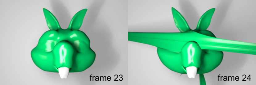
Figure 2: Without line search, the squirrel head animation using our polynomial material (as in Figure 1) quickly becomes unstable.

Alg. 1 summarizes the process of computing one frame of our simulation. The outer loop (lines 2-11) performs quasi-Newton iterations and the inner loop (lines 6-10) implements the line search. What is the extra computational cost required to support more general materials? With Projective Dynamics energies (Eq. 1), we do not need the line search, because $\alpha=1$ always works. Indeed, if we drop the line search from Alg. 1, the algorithm becomes equivalent to a generalized local/global process, as discussed in Section 3 (which is unstable for non-Projective-Dynamics energies). Rejected line search attempts, i.e., additional iterations of the line search, represent the main computational overhead of our method. Fortunately, we found that in practical simulations the number of extra line search iterations is relatively small. For example, in the squirrel head example in Figure 1 using the polynomial material, we need only 4280 line search iterations for the entire sequence with 400 frames, 10 quasi-Newton iterations per frame, i.e., the average number of line search iterations per quasi-Newton iteration is only $1.07$. Even though in most cases the full step ($\alpha=1$) succeeds, the Armijo safeguard is essential for stability; if we drop it, the simulation can quickly explode, as shown in Figure 2.

4.2 Accelerating convergence

The connection between Projective Dynamics and quasi-Newton methods allows us to take advantage of further mathematical optimization techniques. In this section, we discuss how to accelerate convergence of our method using L-BFGS (Limited-memory BFGS). The BFGS algorithm (Broyden-Fletcher-Goldfarb-Shanno) is one of the most popular general purpose quasi-Newton methods; its key idea is to approximate the Hessian using curvature information calculated from previous iterates, i.e., $\mathbf{x}_{1},\dots,\mathbf{x}_{k-1}$. The L-BFGS modification means that we will use only the most recent $m$ iterates, i.e., $\mathbf{x}_{k-m},\dots,\mathbf{x}_{k-1}$; the rationale being that too distant iterates are less relevant in estimating the Hessian at $\mathbf{x}_{k}$.

In Alg. 1, the matrix $\mathbf{M}/h^{2}+\mathbf{L}$ in line 4 can be interpreted as our initial approximation of the Hessian. This matrix is constant which on one hand enables its pre-factorization, but on the other hand, $\mathbf{M}/h^{2}+\mathbf{L}$ may be far from the Hessian $\nabla^{2}g(\mathbf{x}_{k})$, which is the reason for slower convergence compared to Newton’s method [Bouaziz et al. 2014]. L-BFGS allows us to develop a more accurate, state-dependent Hessian approximation, leading to faster convergence without too much computational overhead (in our experiments the overhead is typically less than 1% of the simulation time, see Table 1). The key to fast iterations of L-BFGS is the fact that the progressively updated approximate Hessian $\mathbf{A}_{k}$ is not stored explicitly, which would require us to solve a new linear system $\mathbf{A}_{k}\mathbf{d}(\mathbf{x}_{k})=-\nabla g(\mathbf{x}_{k})$ each iteration, implying high computational costs. Instead, L-BFGS implicitly represents the inverse of $\mathbf{A}_{k}$, i.e., linear operator $\mathbf{B}_{k}$ such that the desired descent direction can be computed simply as $\mathbf{d}(\mathbf{x}_{k})=-\mathbf{B}_{k}\nabla g(\mathbf{x}_{k})$. The linear operator $\mathbf{B}_{k}$ is not represented using a matrix (which would have been dense), but instead as a sequence of dot products, known as the L-BFGS two-loop recursion, see Alg. 2. For a more detailed discussion of BFGS and its variants we refer to Chapters 6 and 7 of [Nocedal and Wright 2006].

1 $\mathbf{q}:=-\nabla g(\mathbf{x}_{k})$

2 for $i=k-1,\dots,k-m$ do

3       $\mathbf{s}_{i}:=\mathbf{x}_{i+1}-\mathbf{x}_{i};\mathbf{t}_{i}:=\nabla g(\mathbf{x}_{i+1})-\nabla g(\mathbf{x}_{i})$; $\rho_{i}:=\mathop{\text{tr}}(\mathbf{t}_{i}^{\mathsf{T}}\mathbf{s}_{i})$

4       $\zeta_{i}:=\mathop{\text{tr}}(\mathbf{s}_{i}^{\mathsf{T}}\mathbf{q})/\rho_{i}$

5       $\mathbf{q}:=\mathbf{q}-\zeta_{i}\mathbf{t}_{i}$

6      

7 end for

8$\mathbf{r}:=\mathbf{A}_{0}^{-1}\mathbf{q}$ // $\mathbf{A}_{0}$ is initial Hessian approximation

9 for $i=k-m,\dots,k-1$ do

10       $\eta:=\mathop{\text{tr}}(\mathbf{t}_{i}^{\mathsf{T}}\mathbf{r})/\rho_{i}$

11       $\mathbf{r}:=\mathbf{r}+\mathbf{s}_{i}(\zeta_{i}-\eta)$

12      

13 end for

14$\mathbf{d}(\mathbf{x}_{k}):=\mathbf{r}$ // resulting descent direction

Algorithm 2 Descent direction computation with L-BFGS

Alg. 2 requires us to provide an initial Hessian approximation $\mathbf{A}_{0}$, ideally such that the linear system $\mathbf{A}_{0}\mathbf{r}=\mathbf{q}$ can be solved efficiently (line 7). In our method, we use our old friend: $\mathbf{M}/h^{2}+\mathbf{L}$. At first, it may seem the initialization of the Hessian is perhaps not too important and the L-BFGS iterations quickly approach the exact Hessian. However, this intuition is not true. In Section 5 we experiment with different possible initializations of the Hessian and show that our particular choice of $\mathbf{M}/h^{2}+\mathbf{L}$ outperforms alternatives such Hessian of the rest-pose and many others. In short, the reason is that the L-BFGS updates use only a very few gradient samples, which provide only a limited amount of information about the exact Hessian. The appeal of the L-BFGS strategy is that it is very fast – the compute cost of the two for-loops in Alg. 2 is negligible compared to the cost of solving the linear system in line 7 with our choice of $\mathbf{A}_{0}=\mathbf{M}/h^{2}+\mathbf{L}$. This is true even for high values of $m$. In other words, the linear solve using $\mathbf{M}/h^{2}+\mathbf{L}$ (line 7) is still doing the “heavy lifting”, while the L-BFGS updates provide additional convergence boost at the cost of minimal computational overheads.

Upgrading our method with L-BFGS is simple: we only need to replace line 4 in Alg. 1 with a call of Alg. 2. Note that for $m=0$, Alg. 2 returns exactly the same descent direction as before, i.e., $\mathbf{d}(\mathbf{x}_{k}):=-(\mathbf{M}/h^{2}+\mathbf{L})^{-1}\nabla{g}(\mathbf{x}_{k})$. What is the optimal $m$, i.e., the size of the history window? Too small $m$ will not allow us to unlock the full potential of L-BFGS. The main problem with too high $m$ is not the higher computational cost of the two loops in Alg. 2, but the fact that too distant iterates (such as $\mathbf{x}_{k-100}$) may contain information irrelevant for the Hessian at $\mathbf{x}_{k}$ and the result can be even worse than with a shorter window. We found that $m=5$ is typically a good value in our experiments.

The recently proposed Chebyshev Semi-Iterative methods for Projective Dynamics [Wang 2015] can also be interpreted as a special type of a quasi-Newton method which utilizes two previous iterates, i.e., corresponding to $m=2$. Indeed, in our experiments L-BFGS with $m=2$ exhibits similar convergence rate as the Chebyshev method, see Figure 6 and further discussion in Section 5. Finally, we note that even though the Wolfe conditions are the recommended line search strategy for L-BFGS, we did not observe any significant convergence benefit compared to our backtracking strategy. However, evaluating the Wolfe conditions increases the computational cost per iteration and therefore, we continue to rely on the backtracking strategy as described in Alg. 1.

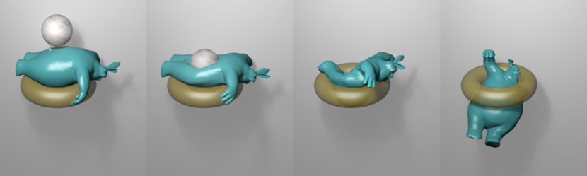
Figure 3: Our method is capable of simulating complex collision scenarios, such as squeezing the Big Bunny through a torus. The Big Bunny uses corotated elasticity with $\mu=5$ and $\lambda=200$.

4.3 Collisions

A classical approach to enforcing non-penetration constraints between deformable solids is to 1) detect collisions and 2) resolve them using temporarily instanced repulsion springs, which bring the volume of undesired overlaps to zero [McAdams et al. 2011, Harmon et al. 2011]. However, in Projective Dynamics the primary emphasis is on computational efficiency and therefore only simplified collision resolution strategies have been proposed by Bouaziz et al. Bouaziz2014Projective. Specifically, Projective Dynamics offers two possible strategies. The first strategy is a two-phase method, where collisions are resolved in a separate post-processing step using projections, similar to Position Based Dynamics. The same strategy was employed also by Liu et al. liu2013fast. The drawback of this approach is the fact the collision projections are oblivious to elasticity and inertia of the simulated objects. The second approach used in Projective Dynamics is more physically realistic, but introduces additional computational overheads. Specifically, temporarily-instanced repulsion springs are added to the total energy. This leads to physically realistic results, but the drawback is that the matrix $\mathbf{M}/h^{2}+\mathbf{L}$ needs to be re-factorized whenever the set of repulsion springs is updated – typically, at the beginning of each frame.

Our quasi-Newton interpretation invites a new approach to collision response which is physically realistic, but avoids expensive re-factorizations. Specifically, for each inter-penetration found by collision detection, we introduce an energy term $E_{\textrm{collision}}(\mathbf{x})=((\mathbf{S}\mathbf{x}-\mathbf{t})^{\mathsf{T}}\mathbf{n})^{2}$, where $\mathbf{S}$ is a selector matrix of the collided vertex, $\mathbf{t}$ is its projection on the surface and $\mathbf{n}$ is the surface normal. This constraint pushes the collided vertex to the tangent plane. It is important to add this term to our total energy $E(\mathbf{x})$ only if the vertex is in collision or contact. Whenever the relative velocity between the vertex and the collider indicates separation, the $E_{\textrm{collision}}(\mathbf{x})$ term is discarded (otherwise it would correspond to unrealistic “glue” forces). This is done once at the beginning of each iteration (just before line 3 in Alg. 1). The line search (lines 6-10 of Alg. 1) is unaffected by these updates, i.e., the unilateral nature of the collision constraints is handled correctly without any further processing.

The key idea of our approach is to leverage the quasi-Newton approximation for collision processing. In particular, we account for the $E_{\textrm{collision}}(\mathbf{x})$ terms when evaluating the energy and its gradients, but we ignore their contributions to the $\mathbf{M}/h^{2}+\mathbf{L}$ matrix. This means that we form a somewhat more aggressive approximation of the Hessian, with the benefit that the system matrix will never need to be re-factorized. The line search process (lines 6-10 in Alg. 1) guarantees that energy will decrease in spite of this more aggressive approximation. The only trade-off we observed in our experiments is that the number of line search iterations may increase, which is a small cost to pay for avoiding re-factorizations. We observed that even in challenging collision scenarios, such as when squeezing a Big Bunny through a torus, the approach behaves robustly and successfully resolves all collisions, see Figure 3.

4.4 Anisotropy

Our numerical methods, including the L-BFGS acceleration, can be directly applied also to anisotropic material models. We verified this on an elastic cube model with corotated base material ($\mu=10$, $\lambda=100$, referring to the notation of Sifakis and Barbič Sifakis2012FEM) enhanced with additional anisotropic stiffness term $\frac{\kappa}{2}(\|\mathbf{F}\mathbf{d}\|-1)^{2}$, where $\mathbf{F}$ is the deformation gradient and $\mathbf{d}$ is the (rest-pose) direction of anisotropy. This corresponds to the directional reinforcement of the material which is common, e.g., in biological soft tissues containing collagenous fibers. The result of our method with $\kappa=50$ can be seen in Figure 4.

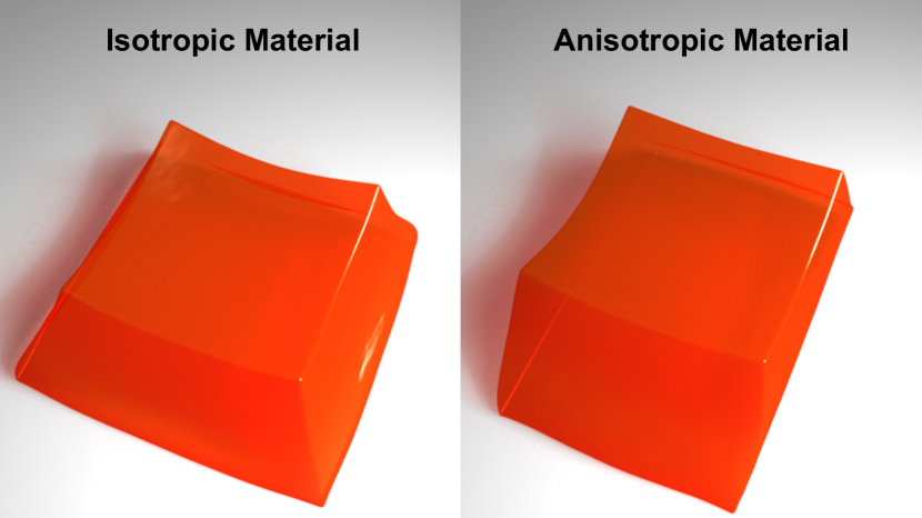
Figure 4: Dropping an elastic cube on the ground. Left: deformation using isotropic elasticity (linear corotated model). Right: the result after adding anisotropic stiffness.

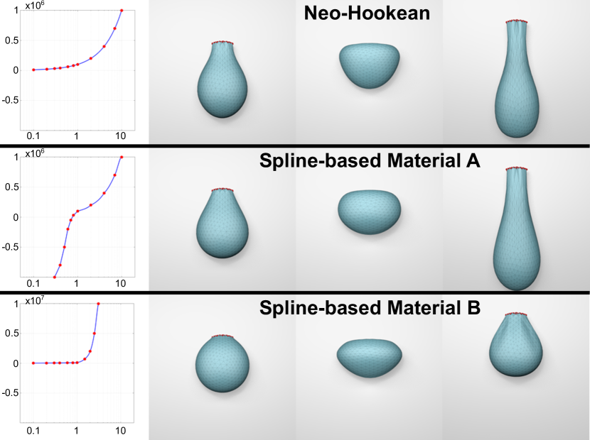
Figure 5: Elastic sphere with spline-based materials [Xu et al. 2015], simulated using our method. Spline-based material A is a modified Neo-Hookean material that resists compression more; material B is a modified Neo-Hookean material that resists tension more. The strain-stress curves are shown on the left.

5 Results

model	#ver.	#ele.	material model	our method (10 iterations)				Newton (1 iteration)
				linesearch	L-BFGS	per-frame	relative	per-frame	relative
				iterations	overhead	time	error	time	error
Thin sheet	660	1932	Polynomial	10.8	0.026 ms	4.4 ms	$2.7\times 10^{-8}$	184 ms	$8.8\times 10^{-4}$
Sphere	889	1821	Spline-based A	24.5†	0.155 ms	21.2 ms	$2.7\times 10^{-7}$	188 ms	$6.9\times 10^{-4}$
Sphere	889	1821	Spline-based B	21.8	0.156 ms	19.7 ms	$6.9\times 10^{-6}$	187 ms	$2.5\times 10^{-4}$
Shaking bar	574	1647	Corotated	10.1	0.193 ms	7.2 ms	$1.6\times 10^{-4}$	171 ms	$4.4\times 10^{-3}$
Ditto	1454	4140	Neo-Hookean	11.7	0.203 ms	17.8 ms	$3.0\times 10^{-5}$	305 ms	$1.6\times 10^{-3}$
Hippo	2387	8406	Corotated	11.9	0.555 ms	40.6 ms	$2.2\times 10^{-3}$	640 ms	$3.7\times 10^{-2}$
Twisting bar	3472	10441	Neo-Hookean	10.6	0.945 ms	45.6 ms	$9.4\times 10^{-5}$	681 ms	$7.9\times 10^{-3}$
Cloth	6561	32160	Mass-Springs	10.0	1.20 ms	42.3 ms	$9.3\times 10^{-4}$	798 ms	$1.2\times 10^{-2}$
Big Bunny	6308	26096	Corotated	49.2‡	2.19 ms	623 ms	$9.8\times 10^{-2}$	2700 ms	$2.8\times 10^{-1}$
Squirrel	8395	23782	Polynomial	10.7	1.41 ms	153 ms	$8.3\times 10^{-8}$	2400 ms	$9.1\times 10^{-6}$
Squirrel	33666	125677	Polynomial	10.5	6.38 ms	706 ms	$1.5\times 10^{-5}$	15800 ms	$5.4\times 10^{-5}$

Table 1: In all examples, we execute 10 iterations of our method per frame, accelerated with L-BFGS with history window $m=5$. Newton’s method uses 1 iteration per frame. The “linesearch iterations” reports the average number of line search iterations per frame. The “L-BFGS overhead” is the runtime overhead of L-BFGS, i.e., timing of Alg. 2 without line 7 ($m=5$). The reported per-frame time for our method accounts for all 10 iterations. One iteration of our method is approximately 100 times faster than one iteration of Newton’s method. We use 10 iterations of our method which reduce the error more than one iteration of Newton’s method, while being about 10 times faster. ^†The higher number of line search iterations is due to the high nonlinearity of the spline-based materials and large deformations of the sphere. ^‡In this case, the higher number of line search iterations is caused by nonlinearities due to collisions (Section 4.3).

Figure 6: Convergence of our method with different L-BFGS history settings, compared to Chebyshev Semi-Iterative method and Newton’s method (baseline). The model is “Twisting bar” with Neo-Hookean elasticity.

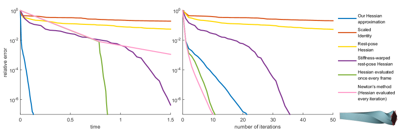
Figure 7: Convergence comparison of L-BFGS methods (all using $m=5$) initialized with different Hessian approximations, along with Newton’s method (baseline). The model is “Twisting bar” with Neo-Hookean elasticity.

Our method supports standard elastic materials, such as corotated linear elasticity, St. Venant-Kirchhoff and the Neo-Hookean model, see Figure Towards Real-time Simulation of Hyperelastic Materials. None of these materials is supported by Projective Dynamics (note that Projective Dynamics supports a special sub-class of corotated linear materials, specifically, ones with $\lambda=0$). Our method also supports the recently introduced spline-based materials proposed by Xu et al. xu2015nonlinear, as shown in Figure Towards Real-time Simulation of Hyperelastic Materials and Figure 5.

Table 1 reports our testing scenarios and compares the run time of our method with Newton’s method, both executed on an Intel i7-4910MQ CPU at 2.90GHz. All scenarios are produced with a fixed timestep of $1/30$ seconds. Because Newton’s method is not guaranteed to work with indefinite Hessians, we employ the standard definiteness fix [Teran et al. 2005], i.e., we project the Hessian of each element to its closest positive definite component. We found this method works better than other definiteness fixes, such as adding a multiple of the identity matrix [Martin et al. 2011], which affects the entire simulation even if there are just a few problematic elements. The approximately 100 times faster run-time of one iteration of our method compared to one iteration of Newton’s method is due to the following facts: 1) we use pre-computed sparse Cholesky factorization, because our matrix $\mathbf{M}/h^{2}+\mathbf{L}$ is constant, 2) the size of our matrix is $n\times n$, whereas the Hessian used in Newton’s method is a $3n\times 3n$ matrix, i.e., the $x,y,z$ coordinates are no longer decoupled, 3) the computation of SVD derivatives, necessary to evaluate the Hessians of materials based on principal stretches [Xu et al. 2015], is expensive. Note that our method is also simpler to implement, as no SVD derivatives or definiteness fixes are necessary.

Comparison to Chebyshev Semi-Iterative method. We compared the convergence of our method with various lengths of the L-BFGS window to the recently introduced Chebyshev Semi-Iterative method [Wang 2015]. We also plot results obtained with Newton’s method as a baseline, see Figure 6.

Even though the Chebyshev method was originally proposed only for Projective Dynamics energies, our generalization to arbitrary materials is compatible with the Chebyshev Semi-Iterative acceleration, see Alg. 3. The Alg. 3 computes a descent direction which can be used in line 4 of Alg. 1. As discussed by Wang wang2015chebyshev, the Chebyshev acceleration should be disabled during the first $S$ iterations, where the recommended value is $S=10$. Another parameter which is essential for the Chebyshev method is an estimate of spectral radius $\rho$, which is calculated from training simulations [Wang 2015]. This parameter must be estimated carefully, because under-estimated $\rho$ can lead to the Chebyshev method producing ascent directions (as opposed to descent directions). Without line search, the ascent directions manifest themselves as oscillations [Wang 2015]. For the purpose of comparisons, we implemented the Chebyshev method with direct solver which is the fastest method on the CPU [Wang 2015].

1 // $S$ …Chebyshev disabled for the first $S$ iterates, default $S$ = 10

2 // $\rho$ …approximated spectral radius

3 $\mathbf{q}:=-(\mathbf{M}/h^{2}+\mathbf{L})^{-1}\nabla{g}(\mathbf{x}_{k})$

4 $\hat{\mathbf{x}}_{k+1}:=\mathbf{x}_{k}+\mathbf{q}$

5 if $k<S$ then $\omega_{k+1}:=1$;

6 if $k=S$ then $\omega_{k+1}:=2/(2-\rho^{2})$;

7 if $k>S$ then $\omega_{k+1}:=4/(4-\rho^{2}\omega_{k})$;

8 $\mathbf{d}(\mathbf{x}_{k}):=\omega_{k+1}(\hat{\mathbf{x}}_{k+1}-\mathbf{x}_{k-1})+\mathbf{x}_{k-1}-\mathbf{x}_{k}$

Algorithm 3 Descent direction computation using Chebyshev Semi-Iterative Method [Wang 2015]

We compare the convergence of all methods using relative error, defined as:

$$\frac{{g}(\mathbf{x}_{k})-{g}(\mathbf{x}^{*})}{{g}(\mathbf{x}_{0})-{g}(\mathbf{x}^{*})}$$ (11)

where $\mathbf{x}_{0}$ is the initial guess (we use $\mathbf{x}_{0}:=\mathbf{y}$ for all methods), $\mathbf{x}_{k}$ is the $k$-th iterate, and $\mathbf{x}^{*}$ is the exact solution computed using Newton’s method (iterated until convergence). The decrease of relative error for one example frame is shown in Figure 6, where all methods are using the backtracking line search outlined in Alg. 1. As expected, descent directions computed using Newton’s method are the most effective ones, as can be seen in Figure 6 (right). However, each iteration of Newton’s method is computationally expensive, and therefore other methods can realize faster error reduction with respect to computational time, as shown in Figure 6 (left). All of the remaining methods are based on the constant Hessian approximation $\mathbf{M}/h^{2}+\mathbf{L}$ which leads to much faster convergence. Out of these methods, classical Projective Dynamics converges slowest. The Chebyshev Semi-Iterative method improves the convergence; we also confirmed that disabling the Chebyshev method during the first 10 iterations indeed helps, as recommended by Wang  wang2015chebyshev. Our method aided with L-BFGS improves convergence even further. Already with $m=2$ (where $m$ is the size of the history window), we obtain slightly faster convergence than with the Chebyshev method. One reason is that it is not necessary to disable L-BFGS in the first several iterates, because L-BFGS is effective as soon as the previous iterates become available. Also, we do not have to estimate the spectral radius which is required by the Chebyshev method. With L-BFGS, we can also increase the history window, e.g., to $m=5$, obtaining even more rapid convergence.

L-BFGS with different initial Hessian estimates. Our method can be interpreted as providing a particularly good initial estimate of the Hessian for L-BFGS. Therefore, it is important to compare to other possible Hessian initializaitons. In a general setting, Nocedal and Wright nocedal2006book recommend to bootstrap L-BFGS using a scaled identity matrix:

$$\mathbf{A}_{0}:=\frac{\mathop{\text{tr}}(\mathbf{s}_{k-1}^{\mathsf{T}}\mathbf{y}_{k-1})}{\mathop{\text{tr}}(\mathbf{y}_{k-1}^{\mathsf{T}}\mathbf{y}_{k-1})}\mathbf{I}$$ (12)

We experimented with this approach, but we found that our choice $\mathbf{A}_{0}:=\mathbf{M}/h^{2}+\mathbf{L}$ leads to much faster convergence, trumping the computational overhead associated with solving the pre-factorized system $\mathbf{A}_{0}\mathbf{r}=\mathbf{q}$ (see Figure 7, red graph).

Another possibility would be to set $\mathbf{A}_{0}$ equal to the rest pose Hessian, which can of course also be pre-factorized. As shown in Figure 7 (yellow graph), this is a slightly better approximation than scaled identity, but still not very effective. This is because the actual Hessian depends on world-space rotations of the model, deviating significantly from the rest-pose Hessian. This issue was observed by Müller et al. Muller2002vertexwarp, who proposed per-vertex stiffness warping as a possible remedy. Per-vertex stiffness warping still allows us to leverage pre-factorization of the rest-pose Hessian and results in better convergence than pure rest-pose Hessian, see Figure 7 (purple graph). However, per-vertex stiffness warping may introduce ghosts forces, because stiffness warping uses different rotation matrices for each vertex, which means that internal forces in one element no longer have to sum to zero. The ghost forces disappear in a fully converged solution, however, this would require a prohibitively high number of iterations.

Yet another possibility is to completely re-evaluate the Hessian at the beginning of each frame. This requires re-factorization, however, the remaining 10 (or so) iterations can reuse the factorization, relying only on L-BFSG updates. When measuring convergence with respect to number of iterations, this approach is very effective, as shown in Figure 7 (right, green graph). However, the cost of the initial Hessian factorization is significant, as obvious from Figure 7 (left, green graph). Our method uses the same Hessian factorization for all frames, avoiding the per-frame factorization costs, while featuring excellent convergence properties, see Figure 7 (blue graph).

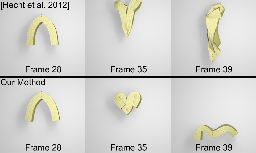
Figure 8: Simulation of a bar with corotated elasticity, constrained in the middle and rapidly shaken. The method of Hecht et al. Hecht:2012:USC with full Hessian updates every other frame explodes due to large ghost forces (top). Our method does not introduce any ghost forces and remains stable (bottom).

The overheads of per-frame Hessian factorizations can be mitigated by carefully scheduled Hessian updates. In particular, the Hessian can be reused for multiple subsequent frames if the state is not changing too much [Deuflhard 2011]. Assuming the corotated elastic model, Hecht et al Hecht:2012:USC push this idea even further by proposing a warp-cancelling form of the Hessian which allows not only for temporal schedule, but also for spatially localized updates. Specifically, a nested dissection tree allows for recomputing only parts of the mesh, which is particularly advantageous in situations where only small part of the object is undergoing large deformations. However, the updates are still costly, and the frequency of the updates depends on the simulation. Similarly to per-vertex stiffness warping, insufficiently frequent update may produce ghost forces and consequent instabilities. This can be a problem when simulating quickly moving elastic objects. To illustrate this, in Figure 8 we show a simulation of shaking an elastic bar. Even if we schedule the Hessian updates every other frame and recompute the entire domain, this method still generates too large ghost forces and becomes unstable. In contrast, our method remains stable and does not require any run-time Hessian updates.

Comparison to Projective Dynamics. One possible alternative to our method would be to apply regular Projective Dynamics with additional strain-limiting constraints [Bouaziz et al. 2014], enabling us to construct piece-wise linear approximations of the strain-stress curves of more general materials. We tried to use this approach to approximate the polynomial material ($a(x)=\mu(x-1)^{4},b(x)=0,c(x)=0$) discussed in Section 4.1, see Figure 9. Even though we obtain similar overall behavior, there are two types of artifacts associated with this approximation. First, the strain-limiting constraints introduce damping when they are not activated. This is because the projection terms still exist in our constant matrix $\mathbf{M}/h^{2}+\mathbf{L}$; if the strain-limiting is not activated, the deformation gradients project to their current values, which produces the undesired damping. The second problem is due to the non-smooth nature of the piece-wise linear approximation, i.e., the stiffness of the simulated object is abruptly changed when the strain-limiting constraints become activated. As shown in the accompanying video, our method avoids both of these issues.

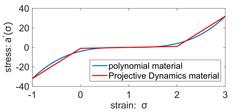
Figure 9: The strain-stress curve of a polynomial material can be approximated piece-wise linearly with two Projective Dynamics constraints.

The L-BFGS acceleration benefits also simulations which use only Projective Dynamics materials (Eq. 1). The most elementary example of these materials are mass-spring systems. In Figure 10, we can see that the L-BFGS acceleration applied to a mass-spring system simulation results in more realistic wrinkles.

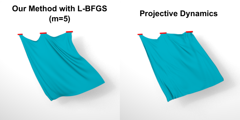
Figure 10: Mass-spring system simulation using our method with L-BFGS (left) and without, i.e., using pure Projective Dynamics (right). The L-BFGS acceleration results in more realistic wrinkles.

Figure 11: Convergence comparison of various methods using sparse direct solvers and conjugate gradients. The model is “Twisting bar” with Neo-Hookean elasticity.

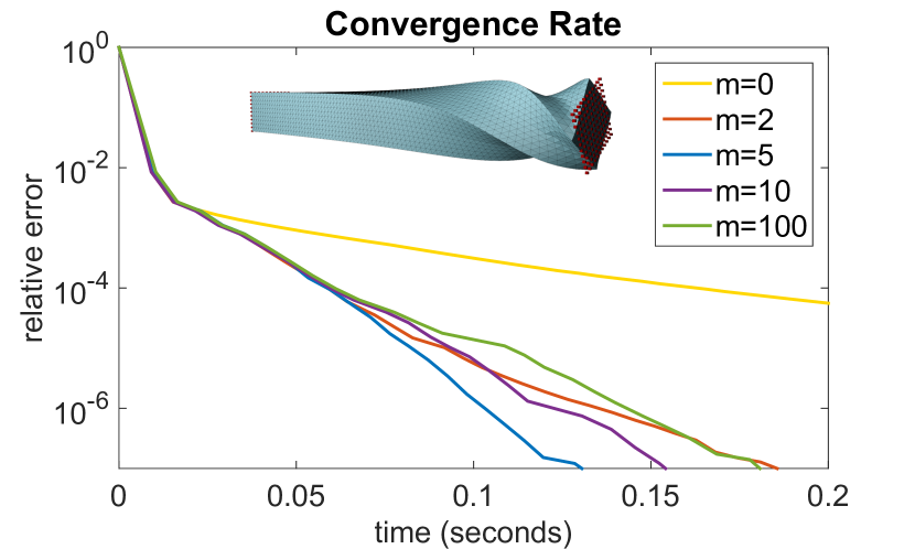
Figure 12: Comparison of L-BFGS convergence rate with different history window sizes ($m$).

Choice of L-BFGS history window size. Which history window ($m$) is the best? We experimented with different values of $m$, see Figure 12. Too large $m$ takes into account too distant iterates which can lead to worse approximation of the Hessian. In Figure 12, we see the optimal value is $m=5$, which is also our recommended default setting. However, it is comforting that the algorithm is not particularly sensitive to the setting of $m$ – even large values such as $m=100$ produce only slightly worse convergence. In Figure 6 we can notice that the convergence rate of the Chebyshev method is similar to our method with L-BFGS using $m=2$. We believe this is not a coincidence, because the Chebyshev method uses two previous iterates, just like L-BFGS with $m=2$.

Figure 13: The convergence rate for different stiffness parameters chosen from different regions.

Choice of stiffness parameters. As discussed in Section 4.1, we Eq. 10 and define our stiffness parameter $k$ as the slope of the best linear approximation of Eq. 10 for $\sigma_{1}\in[x_{\mathrm{start}},x_{\mathrm{end}}]$. What is the best $[x_{\mathrm{start}},x_{\mathrm{end}}]$ interval to use? In the limit, with $[x_{\mathrm{start}},x_{\mathrm{end}}]\rightarrow[1,1]$, our $k$ would converge to the second derivative. However, a finite interval $[x_{\mathrm{start}},x_{\mathrm{end}}]$ guarantees that our $k$ is meaningful even for materials such as the polynomial material $a(x)=\mu(x-1)^{4},b(x)=0,c(x)=0$; in this case, we obtain a $k$ which depends linearly on $\mu$. We argue the convergence of our algorithm is not very sensitive to a particular choice of the $[x_{\mathrm{start}},x_{\mathrm{end}}]$ interval. In Figure 13, we show convergence graphs of a twisting bar with Neo-Hookean material using different intervals to compute the stiffness parameter $k$. Although Neo-Hookean material is highly non-linear, the convergence rates for different interval choices are quite similar. Therefore, we decided not to investigate more sophisticated strategies and we set $x_{\mathrm{start}}=0.5,x_{\mathrm{end}}=1.5$ in all of our simulations.

Comparison with iterative solvers. Sparse iterative solvers do not require expensive factorizations and are therefore attractive in interactive applications. A particularly popular iterative method are Conjugate gradients (CG) [Shewchuk 1994]. An additional advantage is that CG can be implemented in a matrix-free fashion, i.e., without explicitly forming the sparse system matrix. Gast et al. gast2015optimization further accelerate the CG solver used in Newton’s method by proposing a CG-friendly definiteness fix. Specifically, the CG iterations are terminated whenever the maximum number of iteration is reached or indefiniteness of the Hessian matrix is detected.

While iterative methods can be the only possible choice in high-resolution simulations (e.g., in scientific computing), in real-time simulation scales, sparse direct solvers with pre-computed factorization are hard to beat, as we show in Figure 11. Specifically, we test Newton’s method with linear systems solved using CG with 5 and 15 iterations, using Jacobi preconditioner. Even with 15 CG iterations, the accuracy is still not the same as with the direct solver the computational cost becomes high. If we use only five CG iterations the running time improves, but the convergence rate suffers because the descent directions are not sufficiently effective. The method of Gast et al. gast2015optimization initially outperforms Newton with CG, however, the convergence slows down in subsequent iterations. We also tried to apply CG to our method, in lieu of the direct solver. With 15 CG iterations the convergence is competitive, however, the CG solver is slower.

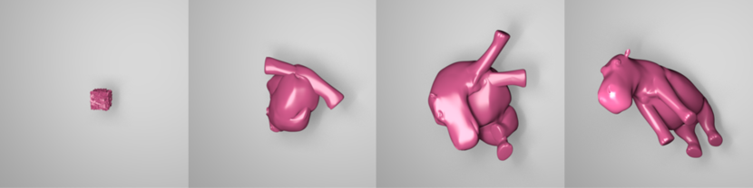
Figure 14: Our method is robust despite extreme initial conditions: a randomly initialized hippo returns back to its rest pose.

Robustness. We demonstrate that our proposed extensions to more general materials and the L-BFGS solver upgrade do not compromise simulation robustness. In Figure 14, we show an elastic hippo which recovers from an extreme (randomized) deformation with many inverted elements. Specifically, the hippo model uses L-BFGS with $m=5$ and corotated linear elasticity with $\mu=20$ and $\lambda=100$ (note that Projective Dynamics supports only corotated materials with $\lambda=0$).

6 Limitations and Future Work

Our method is currently limited only to hyperelastic materials satisfying the Valanis-Landel assumption. Even though this assumption covers many practical models, including the recently proposed spline-based materials [Xu et al. 2015], it would be interesting to study the further generalization of our method. Perhaps even more interesting would be to remove the assumption of hyperelasticity. Can we develop fast algorithms for simulating non-hyperelastic materials, including the effects such as relaxation, creep, and hysteresis [Bargteil et al. 2007]? Inspired by the recent work of Wang wang2015chebyshev, we would like to explore GPU implementations of physics-based simulations. Our current method is derived from the Implicit Euler time integration method and therefore inherits its artificial damping drawbacks. We experimented with Implicit Midpoint – a symplectic integrator which does not suffer from this problem. However, we found that Implicit Midpoint is much less stable. In the future we would like to explore fast numerical solvers for symplectic yet stable integration methods. Finally, we plan to investigate specific physics-based applications which require both high accuracy and speed, such as interactive surgery simulation.

7 Conclusions

We have presented a method for fast physics-based simulation of a large class of hyperelastic materials. The key to our approach is the insight that Projective Dynamics [Bouaziz et al. 2014] can be re-formulated as a quasi-Newton method. Aided with line search, we obtain a robust simulator supporting many practical material models. Our quasi-Newton formulation also allows us to further accelerate convergence by combining our method with L-BFGS. Even though L-BFGS is sensitive to initial Hessian approximation, our method suggests a particularly effective Hessian initialization which yields fast convergence. Most of our experiments use ten iterations of our method which is typically more accurate than one iteration of Newton’s method, while being about ten times faster and easier to implement. Traditionally, real-time physics is considered to be approximate but fast, while off-line physics is accurate but slow. We hope that our method will help to blur the boundaries between real-time and off-line physics-based animation.

Appendix

In this Appendix we compute the gradient $\nabla_{\mathbf{x}}E_{i}(\mathbf{x})$, where $E_{i}(\mathbf{x})$ is defined according to Eq. 1. Dropping the subscript $i$ for clarity, we define the projection:

$$\mathbf{p}(\mathbf{x})=\mathop{\text{argmin }}_{\mathbf{z}\in{\cal{M}}}\|\mathbf{G}\mathbf{x}-\mathbf{z}\|^{2}$$ (13)

where $\mathbf{G}$ represents a discrete differential operator and ${\cal{M}}$ is a constraint manifold. We need to compute the differential:

$$\!\!\!\!\!\!\!\!\!\frac{1}{2}\delta\|\mathbf{G}\mathbf{x}-\mathbf{p}(\mathbf{x})\|^{2} = (\mathbf{G}\mathbf{x}-\mathbf{p}(\mathbf{x}))^{\mathsf{T}}(\mathbf{G}\delta\mathbf{x}-\delta\mathbf{p}(\mathbf{x}))$$ (14)

$$= (\mathbf{G}\mathbf{x}-\mathbf{p}(\mathbf{x}))^{\mathsf{T}}\mathbf{G}\delta\mathbf{x}$$ (15)

because the second term $(\mathbf{G}\mathbf{x}-\mathbf{p}(\mathbf{x}))^{\mathsf{T}}\delta\mathbf{p}(\mathbf{x})$ vanishes. This is due to the fact that $\delta\mathbf{p}(\mathbf{x})\in T_{\mathbf{p}(\mathbf{x})}{\cal{M}}$, where $T_{\mathbf{p}(\mathbf{x})}{\cal{M}}$ denotes the tangent space at point $\mathbf{p}(\mathbf{x})\in{\cal{M}}$. The vector $\mathbf{G}\mathbf{x}-\mathbf{p}(\mathbf{x})$ must be orthogonal to $T_{\mathbf{p}(\mathbf{x})}{\cal{M}}$, otherwise $\mathbf{p}(\mathbf{x})$ could not be the minimizer according to Eq. 13.

References

- [\citenameAn et al. 2008] An, S. S., Kim, T., and James, D. L. 2008. Optimizing cubature for efficient integration of subspace deformations. ACM Trans. Graph..
- [\citenameBarbič and James 2005] Barbič, J., and James, D. L. 2005. Real-time subspace integration for st. venant-kirchhoff deformable models. ACM Trans. Graph..
- [\citenameBargteil et al. 2007] Bargteil, A. W., Wojtan, C., Hodgins, J. K., and Turk, G. 2007. A finite element method for animating large viscoplastic flow. ACM Trans. Graph..
- [\citenameBathe and Cimento 1980] Bathe, K. J., and Cimento, A. P. 1980. Some practical procedures for the solution of nonlinear finite element equations. Computer Methods in Applied Mechanics and Engineering.
- [\citenameBender et al. 2014a] Bender, J., Koschier, D., Charrier, P., and Weber, D. 2014. Position-based simulation of continuous materials. Computers & Graphics.
- [\citenameBender et al. 2014b] Bender, J., Müller, M., Otaduy, M. A., Teschner, M., and Macklin, M. 2014. A survey on position-based simulation methods in computer graphics. In Comput. Graph. Forum.
- [\citenameBouaziz et al. 2012] Bouaziz, S., Deuss, M., Schwartzburg, Y., Weise, T., and Pauly, M. 2012. Shape-up: Shaping discrete geometry with projections. In Comput. Graph. Forum.
- [\citenameBouaziz et al. 2014] Bouaziz, S., Martin, S., Liu, T., Kavan, L., and Pauly, M. 2014. Projective dynamics: Fusing constraint projections for fast simulation. ACM Trans. Graph..
- [\citenameChao et al. 2010] Chao, I., Pinkall, U., Sanan, P., and Schröder, P. 2010. A simple geometric model for elastic deformations. ACM Trans. Graph..
- [\citenameChen et al. 2015] Chen, D., Levin, D., Sueda, S., and Matusik, W. 2015. Data-driven finite elements for geometry and material design. ACM Trans. Graph..
- [\citenameDesbrun et al. 1999] Desbrun, M., Schröder, P., and Barr, A. 1999. Interactive animation of structured deformable objects. Graphics Interface.
- [\citenameDeuflhard 2011] Deuflhard, P. 2011. Newton methods for nonlinear problems: affine invariance and adaptive algorithms. Springer Science & Business Media.
- [\citenameFish et al. 1995] Fish, J., Pandheeradi, M., and Belsky, V. 1995. An efficient multilevel solution scheme for large scale non-linear systems. International Journal for Numerical Methods in Engineering.
- [\citenameFratarcangeli and Pellacini 2015] Fratarcangeli, M., and Pellacini, F. 2015. Scalable partitioning for parallel position based dynamics. Comput. Graph. Forum.
- [\citenameGast et al. 2015] Gast, T. F., Schroeder, C., Stomakhin, A., Jiang, C., and Teran, J. M. 2015. Optimization integrator for large time steps. Visualization and Comp. Graph., IEEE Transactions on.
- [\citenameGeorgii and Westermann 2006] Georgii, J., and Westermann, R. 2006. A multigrid framework for real-time simulation of deformable bodies. Computers & Graphics 30, 3, 408–415.
- [\citenameGoldenthal et al. 2007] Goldenthal, R., Harmon, D., Fattal, R., Bercovier, M., and Grinspun, E. 2007. Efficient simulation of inextensible cloth. ACM Trans. Graph..
- [\citenameHahn et al. 2012] Hahn, F., Martin, S., Thomaszewski, B., Sumner, R., Coros, S., and Gross, M. 2012. Rig-space physics. ACM Trans. Graph..
- [\citenameHairer et al. 2002] Hairer, E., Lubich, C., and Wanner, G. 2002. Geometric Numerical Integration: Structure-Preserving Algorithms for Ordinary Differential Equations. Springer.
- [\citenameHarmon and Zorin 2013] Harmon, D., and Zorin, D. 2013. Subspace integration with local deformations. ACM Trans. Graph..
- [\citenameHarmon et al. 2011] Harmon, D., Panozzo, D., Sorkine, O., and Zorin, D. 2011. Interference-aware geometric modeling. In ACM Trans. Graph.
- [\citenameHauth and Etzmuss 2001] Hauth, M., and Etzmuss, O. 2001. A high performance solver for the animation of deformable objects using advanced numerical methods. In Comput. Graph. Forum.
- [\citenameHecht et al. 2012] Hecht, F., Lee, Y. J., Shewchuk, J. R., and O’Brien, J. F. 2012. Updated sparse cholesky factors for corotational elastodynamics. ACM Trans. Graph..
- [\citenameIrving et al. 2004] Irving, G., Teran, J., and Fedkiw, R. 2004. Invertible finite elements for robust simulation of large deformation. In Proc. EG Symp. Computer Animation.
- [\citenameKharevych et al. 2006] Kharevych, L., Yang, W., Tong, Y., Kanso, E., Marsden, J. E., Schröder, P., and Desbrun, M. 2006. Geometric, variational integrators for computer animation. In Proc. EG Symp. Computer Animation.
- [\citenameKim et al. 2012] Kim, T.-Y., Chentanez, N., and Müller-Fischer, M. 2012. Long range attachments-a method to simulate inextensible clothing in computer games. In Proc. EG Symp. Computer Animation.
- [\citenameLi et al. 2014] Li, S., Huang, J., de Goes, F., Jin, X., Bao, H., and Desbrun, M. 2014. Space-time editing of elastic motion through material optimization and reduction. ACM Trans. Graph..
- [\citenameLiu et al. 2013] Liu, T., Bargteil, A. W., O’Brien, J. F., and Kavan, L. 2013. Fast simulation of mass-spring systems. ACM Trans. Graph..
- [\citenameMacklin and Müller 2013] Macklin, M., and Müller, M. 2013. Position based fluids. ACM Trans. Graph..
- [\citenameMacklin et al. 2014] Macklin, M., Müller, M., Chentanez, N., and Kim, T.-Y. 2014. Unified particle physics for real-time applications. ACM Trans. Graph..
- [\citenameMartin et al. 2011] Martin, S., Thomaszewski, B., Grinspun, E., and Gross, M. 2011. Example-based elastic materials. In ACM Trans. Graph.
- [\citenameMartin et al. 2013] Martin, T., Joshi, P., Bergou, M., and Carr, N. 2013. Efficient non-linear optimization via multi-scale gradient filtering. In Comput. Graph. Forum.
- [\citenameMcAdams et al. 2011] McAdams, A., Zhu, Y., Selle, A., Empey, M., Tamstorf, R., Teran, J., and Sifakis, E. 2011. Efficient elasticity for character skinning with contact and collisions. ACM Trans. Graph..
- [\citenameMüller and Chentanez 2011] Müller, M., and Chentanez, N. 2011. Solid simulation with oriented particles. In ACM Trans. Graph.
- [\citenameMüller and Gross 2004] Müller, M., and Gross, M. 2004. Interactive virtual materials. In Proceedings of Graphics Interface.
- [\citenameMüller et al. 2002] Müller, M., Dorsey, J., McMillan, L., Jagnow, R., and Cutler, B. 2002. Stable real-time deformations. In Proc. EG Symp. Computer Animation.
- [\citenameMüller et al. 2005] Müller, M., Heidelberger, B., Teschner, M., and Gross, M. 2005. Meshless deformations based on shape matching. In ACM Trans. Graph.
- [\citenameMüller et al. 2007] Müller, M., Heidelberger, B., Hennix, M., and Ratcliff, J. 2007. Position based dynamics. J. Vis. Comun. Image Represent..
- [\citenameMüller et al. 2014] Müller, M., Chentanez, N., Kim, T.-Y., and Macklin, M. 2014. Strain based dynamics. In Proc. EG Symp. Computer Animation, vol. 2.
- [\citenameMüller et al. 2015] Müller, M., Chentanez, N., Kim, T.-Y., and Macklin, M. 2015. Air meshes for robust collision handling. ACM Trans. Graph..
- [\citenameMüller 2008] Müller, M. 2008. Hierarchical Position Based Dynamics. In Workshop in Virtual Reality Interactions and Physical Simulation "VRIPHYS" (2008), The Eurographics Association.
- [\citenameNarain et al. 2012] Narain, R., Samii, A., and O’Brien, J. F. 2012. Adaptive anisotropic remeshing for cloth simulation. ACM Trans. Graph..
- [\citenameNeuberger 1983] Neuberger, J. 1983. Steepest descent for general systems of linear differential equations in hilbert space. In Ordinary differential equations and operators. Springer.
- [\citenameNeuberger 2009] Neuberger, J. 2009. Sobolev gradients and differential equations. Springer Science & Business Media.
- [\citenameNocedal and Wright 2006] Nocedal, J., and Wright, S. J. 2006. Numerical optimization. Springer Verlag.
- [\citenameRivers and James 2007] Rivers, A., and James, D. 2007. FastLSM: fast lattice shape matching for robust real-time deformation. ACM Trans. Graph..
- [\citenameServin et al. 2006] Servin, M., Lacoursière, C., and Melin, N. 2006. Interactive simulation of elastic deformable materials. In SIGRAD.
- [\citenameShewchuk 1994] Shewchuk, J. R., 1994. An introduction to the conjugate gradient method without the agonizing pain.
- [\citenameSifakis and Barbič 2012] Sifakis, E., and Barbič, J. 2012. Fem simulation of 3d deformable solids: A practitioner’s guide to theory, discretization and model reduction. In ACM SIGGRAPH Courses.
- [\citenameStam 2009] Stam, J. 2009. Nucleus: towards a unified dynamics solver for computer graphics. In IEEE Int. Conf. on CAD and Comput. Graph.
- [\citenameTamstorf et al. 2015] Tamstorf, R., Jones, T., and McCormick, S. F. 2015. Smoothed aggregation multigrid for cloth simulation. ACM Trans. Graph..
- [\citenameTeng et al. 2014] Teng, Y., Otaduy, M. A., and Kim, T. 2014. Simulating articulated subspace self-contact. ACM Trans. Graph..
- [\citenameTeng et al. 2015] Teng, Y., Meyer, M., DeRose, T., and Kim, T. 2015. Subspace condensation: Full space adaptivity for subspace deformations. ACM Trans. Graph..
- [\citenameTeran et al. 2005] Teran, J., Sifakis, E., Irving, G., and Fedkiw, R. 2005. Robust quasistatic finite elements and flesh simulation. In Proc. EG Symp. Computer Animation.
- [\citenameTerzopoulos et al. 1987] Terzopoulos, D., Platt, J., Barr, A., and Fleischer, K. 1987. Elastically deformable models. In Computer Graphics (Proceedings of SIGGRAPH).
- [\citenameThomaszewski et al. 2009] Thomaszewski, B., Pabst, S., and Straßer, W. 2009. Continuum-based strain limiting. In Comput. Graph. Forum.
- [\citenameTournier et al. 2015] Tournier, M., Nesme, M., Gilles, B., and Faure, F. 2015. Stable constrained dynamics. ACM Trans. Graph..
- [\citenameValanis and Landel 1967] Valanis, K., and Landel, R. 1967. The strain-energy function of a hyperelastic material in terms of the extension ratios. Journal of Applied Physics.
- [\citenameWang et al. 2010] Wang, H., O’Brien, J., and Ramamoorthi, R. 2010. Multi-resolution isotropic strain limiting. ACM Trans. Graph..
- [\citenameWang 2015] Wang, H. 2015. A chebyshev semi-iterative approach for accelerating projective and position-based dynamics. ACM Trans. Graph..
- [\citenameXu et al. 2015] Xu, H., Sin, F., Zhu, Y., and Barbič, J. 2015. Nonlinear material design using principal stretches. ACM Trans. Graph..