Bayesian Modelling and Quantification of Raman Spectroscopy

Abstract

Raman spectroscopy can be used to identify molecules such as DNA by the characteristic scattering of light from a laser. It is sensitive at very low concentrations and can accurately quantify the amount of a given molecule in a sample. The presence of a large, nonuniform background presents a major challenge to analysis of these spectra. To overcome this challenge, we introduce a sequential Monte Carlo (SMC) algorithm to separate each observed spectrum into a series of peaks plus a smoothly-varying baseline, corrupted by additive white noise. The peaks are modelled as Lorentzian, Gaussian, or pseudo-Voigt functions, while the baseline is estimated using a penalised cubic spline. This latent continuous representation accounts for differences in resolution between measurements. The posterior distribution can be incrementally updated as more data becomes available, resulting in a scalable algorithm that is robust to local maxima. By incorporating this representation in a Bayesian hierarchical regression model, we can quantify the relationship between molecular concentration and peak intensity, thereby providing an improved estimate of the limit of detection, which is of major importance to analytical chemistry.

Keywords: chemometrics; functional data analysis; multivariate calibration; nanotechnology; sequential Monte Carlo

1 Introduction

Raman spectroscopy has many emerging and existing applications in biomedical research (Ellis et al., 2013; Butler et al., 2016). For example, a Raman-active dye label can be attached to an antibody targeting a specific biomarker, such as a protein or DNA sequence. The concentration of that biomarker can then be quantified within a living organism (Zavaleta et al., 2009; Laing et al., 2017). This enables disease diagnosis and imaging of biological process at the molecular level, with a high degree of specificity. Raman spectroscopy can be performed noninvasively and nondestructively, offering substantial advantages over alternative techniques such as immunofluorescence. Raman scattering produces a complex pattern of peaks, which correspond to the vibrational modes of the molecule. This spectral signature is highly specific, enabling simultaneous identification and quantification of several molecules in a multiplex (Zhong et al., 2011; Gracie et al., 2014).

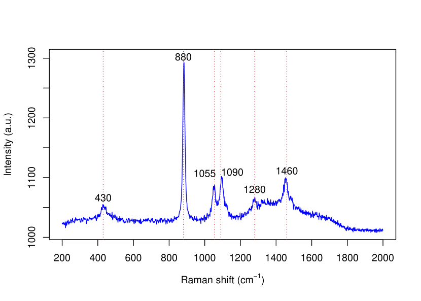
Figure 1: Raman spectrum of ethanol, showing the locations of 6 major peaks (430, 880, 1055, 1090, 1280 & 1460 cm^-1).

In this paper, we introduce a model-based approach for quantification of Raman spectroscopy. An example Raman spectrum for ethanol (EtOH) is shown in Fig. 1. Here we are focused on the fingerprint region for organic molecules: wavenumbers $\Delta\tilde{\nu}$ in the range 200 to 2000 cm^-1 containing the characteristic Raman peaks. The vertical axis is measured in arbitrary units (a.u.), since the observed signal intensity is dependent on the calibration of the spectrometer, among several other factors. EtOH is a relatively simple molecule in comparison to the Raman-active dye labels that are used in biomedical applications, such as those described in Sect. 2. The 6 major peaks in its spectral signature can be directly attributed to vibrational modes of the bonds between its 9 atoms (Mammone et al., 1980; Lin-Vien et al., 1991). Most of these peaks are well-separated, so that the shape of the smooth baseline function can be easily discerned.

A further advantage of Raman spectroscopy is that the amplitudes of the peaks increase linearly with the concentration of the molecule (Jones et al., 1999). A dilution study can be performed to measure Raman spectra at a range of known concentrations. By fitting a linear regression model to this data, it is then possible to estimate the limit of detection (LOD) for the molecule, which is the minimum concentration that the Raman peaks can be distinguished from noise:

$$c_{LOD}=\frac{3\sigma_{\epsilon}}{\beta_{p}}$$ (1)

where $\sigma_{\epsilon}$ is the standard deviation of the additive white noise and $\beta_{p}$ is the linear regression coefficient for peak $p$. The LOD is usually only estimated for the single, largest peak (univariate calibration). For example, the LOD for the EtOH peak at 880 cm^-1 has been estimated as 1.2 millimolar (mM) concentration (Boyaci et al., 2012). This can be used to estimate the alcohol content of commodity spirits, such as whisky, vodka, or gin, as well as to detect counterfeits (Ellis et al., 2017).

More complex molecules might not have a single, dominant peak that is well-separated from the others. In this case, multivariate calibration (MVC) can be used to quantify several peaks simultaneously (Pelletier, 2003; Varmuza and Filzmoser, 2009). Traditional chemometric methods for MVC include direct classical least squares (DCLS: Haaland and Easterling, 1980). However, DCLS relies on accurate baseline subtraction as a data pre-processing step, which is a painstaking and subjective process for the chemist to perform manually themselves.

Existing approaches to automated baseline correction include asymmetric least squares (Boelens et al., 2005; He et al., 2014), iterative polynomial fit (Lieber and Mahadevan-Jansen, 2003; Gan et al., 2006), locally weighted smoothing (Ruckstuhl et al., 2001), and wavelet decomposition (Cai et al., 2001; Galloway et al., 2009). See Liland et al. (2010) for a comparative review. Subtracting the baseline as a pre-processing step ignores the uncertainty in the estimate, where several candidate baselines might fit the data equally well. This can introduce artefacts that cause bias in the resulting quantification, since the remaining signal can have very low likelihood, once the shape of the peaks is taken into account. This is particularly a problem for Raman spectra of complex molecules, where the peaks overlap to such a degree that the baseline is seldom directly observed. It would be preferable to estimate the parameters of both the peaks and the baseline jointly, since uncertainty about the baseline can then be incorporated into the overall estimate.

An iterative algorithm for estimation of the baseline and peaks was introduced by De Rooi and Eilers (2012). They combined a penalised spline for the baseline with a mixture model to differentiate between the peaks and the residual noise. The noise was assumed to be Gaussian, while the peaks were represented using a uniform distribution on the positive real numbers. This nonparametric model does not assume any functional form for the broadening of the peaks. Thus, it cannot be used to estimate quantities of scientific interest, such as the LOD in (1). Treating the peaks as an unordered collection of points also ignores dependence between neighbouring values in the spectrum and makes it difficult to compare spectra with different discretisations (resolution of the horizontal axis).

Alternatively, each peak could be represented as a continuous function, in accordance with the known physical properties of Raman spectroscopy. Doppler broadening is a result of the emitted photons being red (blue) shifted due to particles moving away from (towards) the sensor. Since the particles are undergoing Brownian motion, this gives rise to a symmetric, radial basis function (RBF):

$$f_{G}(\nu_{j}\mid\ell_{p},\psi_{p})\propto\exp\left\{-\frac{(\nu_{j}-\ell_{p})^{2}}{2\psi_{p}^{2}}\right\}$$ (2)

where $\nu_{j}$ is the $j$th wavenumber in the spectrum, $\ell_{p}$ is the location of peak $p$, and $\psi_{p}$ is a scale parameter that controls the width of the peak. RBF peaks are sometimes referred to as Gaussian or squared exponential, but we use the term RBF in this paper to distinguish these functions from the use of the Gaussian probability distribution, for example in the additive white noise. The full width at half maximum (FWHM) of a RBF peak can be calculated as $2\psi_{p}\sqrt{2\ln 2}$.

Collisional broadening occurs due to collisions between particles, which effectively lower the characteristic time of the emission process. As a result of the uncertainty principle this increases the uncertainty in the energy of the emitted photons, which is described by a Lorentzian function:

$$f_{L}(\nu_{j}\mid\ell_{p},\gamma_{p})\propto\frac{\gamma_{p}^{2}}{(\nu_{j}-\ell_{p})^{2}+\gamma_{p}^{2}}$$ (3)

The FWHM of a Lorenztian peak is given by $2\gamma_{p}$. This function has the form of an unnormalised Cauchy density, but again we prefer the term Lorentzian to distinguish from the probability distribution. The heavier tails of the Lorentzian would imply long-range dependence between peaks. Failure to account for this would introduce bias, particularly if quantification was based on a single peak in isolation.

Often the observed spectrum is the result of a combination of the above processes. This can be represented as a Voigt function, which is the convolution of a RBF and a Lorentzian:

$$f_{V}(\nu_{j})=(f_{G}*f_{L})(\nu_{j})=\int_{-\infty}^{+\infty}f_{G}(\tilde{\nu})f_{L}(\nu_{j}-\tilde{\nu})\,d\tilde{\nu}$$ (4)

Since the result of this convolution is unavailable in closed form, (4) is usually approximated by an additive Gaussian-Lorentzian function, also known as a pseudo-Voigt (Wertheim and Dicenzo, 1985):

$$f_{V}(\nu_{j})\approx\tilde{f}_{V}(\nu_{j}\mid\ell_{p},\psi_{p},\gamma_{p})=\eta_{p}f_{L}(\nu_{j}\mid\ell_{p},\gamma_{p})+(1-\eta_{p})f_{G}(\nu_{j}\mid\ell_{p},\psi_{p})$$ (5)

where the mixing proportion $0\leq\eta_{p}\leq 1$ is determined by the scale parameters $\psi_{p}$ and $\gamma_{p}$ (Thompson et al., 1987; Ida et al., 2000). $\eta_{p}=0$ is equivalent to a pure RBF, while $\eta_{p}=1$ is equivalent to a Lorentzian. Thus, $\eta_{p}$ can be viewed as averaging between the two alternative models.

Parametric functional models such as these have previously been applied to other types of spectroscopy. Ritter (1994) introduced a Bayesian model for the peaks in electron spectroscopy, using pseudo-Voigt functions for the broadening. Ritter derived informative priors for the locations, FWHM, and mixing proportions of the peaks. This model was fitted to four peaks, removing the baseline as a pre-processing step. van Dyk et al. (2001); van Dyk and Kang (2004) developed a joint model for the baseline and peaks in X-ray and $\gamma$-ray astronomy, using RBF broadening. This model is specifically suited to data with low photon counts, where the additive white noise assumption is inappropriate.

Fischer and Dose (2002) and Razul et al. (2003) introduced reversible-jump Markov chain Monte Carlo (RJ-MCMC) algorithms (Green, 1995) when the number of peaks is unknown. The baseline was estimated using a penalised spline, as in De Rooi and Eilers (2012), but the peaks were modelled using RBF broadening (2). The number and locations of both the knots and the peaks were determined by the trans-dimensional algorithm. Wang et al. (2008) used RJ-MCMC to fit a similar model to mass spectrometry. These methods have only been applied to spectra where the baseline function is highly regular, or where the peaks are spaced far enough apart that the baseline can be directly observed.

Peak detection is less important in Raman spectroscopy, since there are abundant sources of information on the numbers and locations of the peaks. Time-dependent density functional theory (TD-DFT; Van Caillie and Amos, 2000; Jensen et al., 2008) can be used to predict peak locations from the chemical structure of a molecule. Examples of molecules with predicted Raman spectra include rhodamine 6G (Watanabe et al., 2005), crystal violet (Kleinman et al., 2011), eosin-Y (Greeneltch et al., 2012) and II-MB-114 (Kearns et al., 2016). There are also databases available of known Raman spectra, such as RRUFF (Lafuente et al., 2015), SDBS (AIST, 2001), and the Raman Spectroscopic Library of Natural and Synthetic Pigments (Bell et al., 1998).

Recently, Frøhling et al. (2016) applied a joint model of peaks and baseline to Raman spectroscopy. They used pseudo-Voigt functions for the broadening of the peaks, but assumed a linear baseline. This simplified baseline was only feasible because the model was fitted to a small window of the spectrum, where the baseline was approximately flat. It would not be applicable to the more complex datasets that we analyse in this paper, since our aim is to analyse all of the peaks in the spectral signature of a molecule.

The primary contribution of this paper is a hierarchical regression model for multivariate calibration (MVC). We extend the previous models of peaks and baselines in spectroscopy to obtain estimates of the relationship between molecular concentration and amplitude for each peak. Our model provides posterior distributions for quantities of scientific interest, such as FWHM and LOD. This is the first paper to use computational predictions from TD-DFT as an informative prior for analysis of observed spectra. We introduce a sequential Monte Carlo (SMC) algorithm (Chopin, 2002; Del Moral et al., 2006) to fit our model to large spectral datasets. We have implemented this algorithm as an open-source software package for the R statistical computing platform (R Core Team, 2017).

The remainder of this article is organised as follows. Sect. 2 contains a description of the Raman spectroscopic data. We present our hierarchical regression model and informative priors in Sect. 3. Our SMC algorithm for fitting this model is described in Sect. 4. Results of applying our method to Raman spectroscopy are presented in Sect. 5. We conclude the article with a discussion.

2 Experimental Data

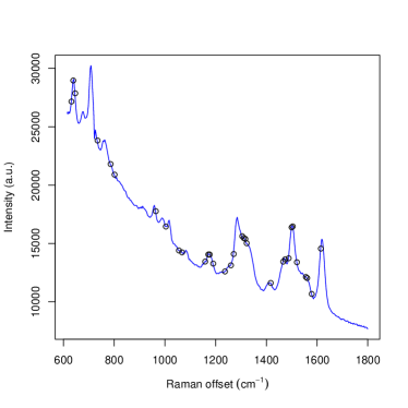
(a) Eosin.

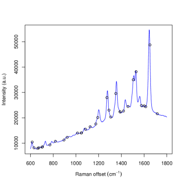
(b) Rhodamine B.

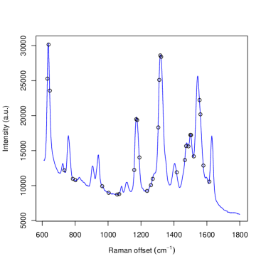
(c) FAM.

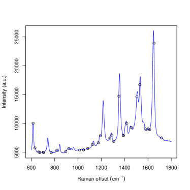
(d) TAMRA.

Figure 2: Surface-enhanced Raman scattering (SERS) spectra for eosin, rhodamine B, fluorescein (FAM), and tetramethylrhodamine (TAMRA). The dots show the 32 peak locations predicted using time-dependent density functional theory (TD-DFT) for eosin and rhodamine.

We analyse two spectroscopic datasets in this paper. In both cases, we have used metallic nanoparticles to enhance the Raman signal. This is known as surface-enhanced Raman scattering (SERS; Le Ru and Etchegoin, 2009). Specifically, we used citrate-reduced silver nanoparticles (Ag NP) with mean diameter of 78 nm.

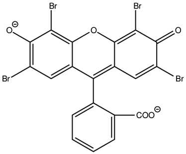
(a) Eosin.

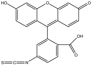
(b) FAM.

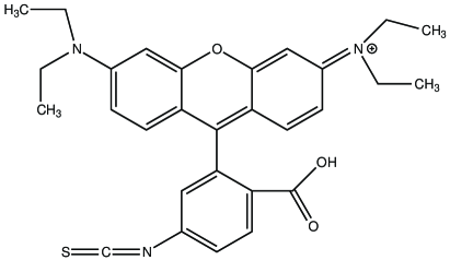
(c) Rhodamine B.

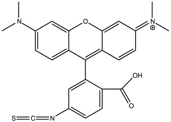
(d) TAMRA.

Figure 3: Chemical structures of eosin, fluorescein (FAM), rhodamine B, and tetramethylrhodamine (TAMRA).

The first dataset contains 15 spectra (5 repeat scans of 3 technical replicates) for each of 4 Raman-active dye molecules: eosin, fluorescein (FAM), rhodamine B, and tetramethylrhodamine (TAMRA). As previously mentioned, computational predictions for the locations of the eosin peaks using TD-DFT have been published by Greeneltch et al. (2012). They predicted 32 peaks between 631.6 and 1615 cm^-1. An observed spectrum, with the predicted peak locations marked, is shown in Fig. 2a. Eosin and FAM are closely related, as illustrated by their chemical structures in Figs 3a and 3b, respectively. Therefore, we might expect that the spectral signatures of these two dyes would be similar to each other. This is not clear from the observed spectrum in Fig. 2c due to the large difference in the shape of the baseline. However, the 32 predicted locations appear to be in approximately the right place. The 32 points in Fig. 2b show the peak locations predicted using TD-DFT by Watanabe et al. (2005). Rhodamine and TAMRA are also closely related, as shown by their chemical structures in Figs 3c and 3d, so we use the same priors for both dyes. An observed spectrum for TAMRA is shown in Fig. 2d. Both the peaks and the baselines of these molecules are far more complex than for EtOH in Fig. 1. This illustrates why more advanced methods are needed for analysis of these spectra.

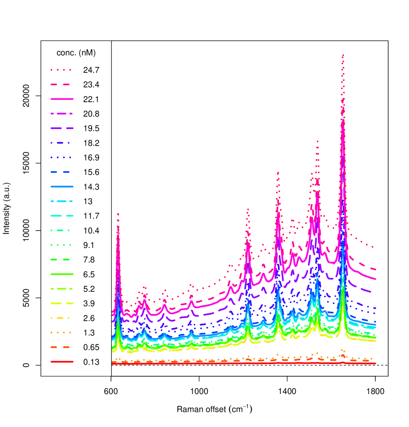
Figure 4: Dilution study for tetramethylrhodamine (TAMRA), showing the average spectrum at each of 21 concentrations from 0.13 to 24.7 nM.

The second dataset is a dilution study for TAMRA: spectra have been obtained for 21 different concentrations, from 0.13 to 24.7 nanomolar (nM). These data were originally analysed by Gracie et al. (2014). There are 5 repeats of 3 technical replicates at each concentration, giving a total sample size of 315 spectra. These spectra were obtained using a 100 mW laser at 532 nm excitation wavelength. The resolution of the spectrometer was 0.5 cm^-1, providing 2401 measurements between 600 and 1800 cm^-1. The average of the observed spectrum at each concentration is shown in Fig. 4. Gracie et al. previously used univariate calibration to estimate a LOD of 99.5 picomolar (pM) for the peak at 1650 cm^-1. The aim of our analysis is to estimate the LOD of all 32 peaks simultaneously, using a Bayesian MVC approach.

3 Hierarchical Model

A Raman spectrum is discretised into a multivariate observation that is highly collinear, hence it lends itself to a reduced-rank representation. Our approach is a form of functional data analysis (Ramsay and Silverman, 2005), where the observed signal is represented using continuous functions. We decompose the spectrum into three major components:

$$y_{i}(\tilde{\nu})=\xi_{i}(\tilde{\nu})+s_{i}(\tilde{\nu})+\boldsymbol{\epsilon}$$ (6)

where $y_{i}(\tilde{\nu})$ is a hyperspectral observation that has been discretised at a number of light frequencies or wavenumbers, $\nu_{j}\in\tilde{\nu}$. Multiple observations are represented as a matrix $[\mathbf{Y}]_{1:n_{y},1:n_{\tilde{\nu}}}$. The spectral signature $s_{i}(\tilde{\nu})$ comprises the Raman peaks and $\xi_{i}(\tilde{\nu})$ is the baseline. We assume that $\boldsymbol{\epsilon}$ is zero mean, additive white noise with constant variance:

$$\epsilon_{i,j}\sim\mathcal{N}\left(0,\sigma^{2}_{\epsilon}\right)$$ (7)

This assumption could be relaxed by allowing for autocorrelated residuals, as in Chib (1993).

The baseline is a smoothly-varying, continuous function that is mainly due to background fluorescence. The shape of the baseline can vary considerably between experiments and even occasionally between technical replicates. The main property that distinguishes the baseline from the other components of the signal is its smoothness. For this reason, we have chosen to model the baseline function as a penalised B-spline (Eilers and Marx, 1996):

$$\xi_{i}(\tilde{\nu})=\sum_{m=1}^{M}B_{m}(\tilde{\nu})\alpha_{i,m}$$ (8)

where $B_{m}$ are the basis functions, $M$ is the total number of splines, and $\alpha_{i,m}$ are the coefficients of the baseline for the $i$th observation. We use equally-spaced knots 10 cm^-1 apart, so that $M$ is typically $\approx$ 120. If the choice of knot locations is a concern, then a smoothing spline (Eubank, 1999) could be used instead. Razul et al. (2003) used an RJ-MCMC algorithm to determine the number and placement of the knots in the baseline function.

As with many Bayesian regression models, (8) can be interpreted as a type of Gaussian process (GP; Rasmussen and Williams, 2006, ch. 6). An advantage of our approach is that we employ a reduced-rank representation of the baseline function. The computational cost of estimating the spline parameters $\alpha_{i,m}$ using sparse matrix algebra is $\mathcal{O}\left(n\right)$ (Green and Silverman, 1994). This is far more scalable than the usual GP methods, which require $\mathcal{O}\left(n^{3}\right)$ operations to invert the covariance matrix. Alternative methods for fast GP fitting include the fixed-rank kriging of Cressie and Johannesson (2008), the Markov random field representation of Lindgren et al. (2011), and the nearest-neighbour GP of Datta et al. (2016).

The Raman peaks are represented as an additive mixture of broadening functions. We follow Ritter (1994); Frøhling et al. (2016) in using pseudo-Voigt functions:

$$s_{i}(\nu_{j})=\sum_{p=1}^{P}A_{i,p}\,\tilde{f}_{V}(\nu_{j}\mid\ell_{p},\psi_{p},\gamma_{p})$$ (9)

where $A_{i,p}$ is the amplitude or height of peak $p$ in the $i$th observation. The other parameters are as defined in (5). RBF (2) or Lorentzian (3) broadening functions can be viewed as special cases of the pseudo-Voigt. We extend the previous functional models of spectroscopy by modelling the dependence of the amplitudes on the concentration of the molecule:

$$A_{i,p}=c_{i}\beta_{p},\qquad c_{LOD}<c_{i}<c_{MLC}$$ (10)

The regression coefficients $\beta_{p}$ can be estimated using dilution studies, such as the dataset described in Sect. 2. Given a posterior distribution for $\beta_{p}$ and the other parameters, an unknown concentration $c_{i}$ can then be estimated for subsequent observations of the same molecule.

The minimum concentration $c_{LOD}$ is as defined in (1), the point at which the peak is indistinguishable from the noise $\sigma_{\epsilon}$. Monolayer coverage $c_{MLC}$ is the saturation point, where increasing the dye concentration does not result in any increase in signal intensity. Jones et al. (1999) calculated that a final concentration of 10 nM is required for monolayer coverage of silver nanoparticles with average diameter of 27 nm. The spectra that we analyse in Sect. 5 were obtained using much larger nanoparticles, with average diameter of 78 nm, therefore we would expect $c_{MLC}$ to be higher for this dataset. We do not observe any evidence of saturation in our spectra, even for concentrations up to 24.7 nM.

3.1 Priors

We used the predicted peak locations from TD-DFT as informative priors for the first dataset, as illustrated in Fig. 2:

$$\pi(\ell_{p})\sim\mathcal{N}(pred_{p},\sigma^{2}_{pred})$$ (11)

The uncertainty in these predictions was estimated from the differences between predicted and observed peak locations that were reported by Greeneltch et al. (2012) and Watanabe et al. (2005).

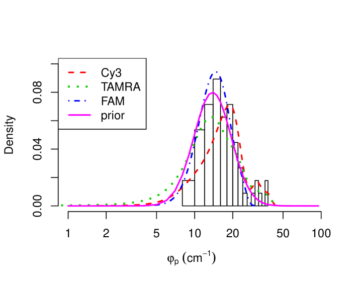
(a) Prior for radial basis function broadening.

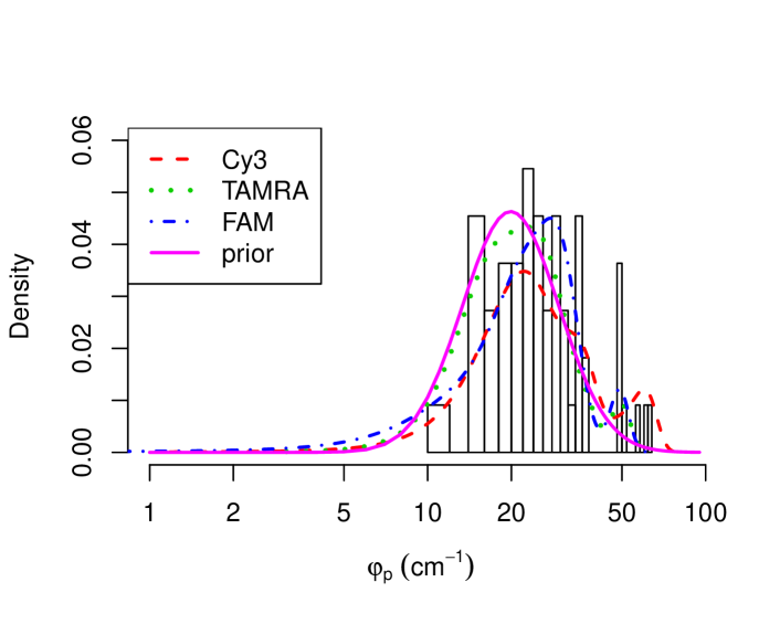
(b) Prior for Lorentzian broadening.

Figure 5: Informative priors for the scale parameters of Raman peaks, derived from manual baseline correction and peak fitting of Cy3, TAMRA and FAM spectra using Grams/AI 7.00.

We derived informative priors for the scale parameters $\psi_{p}$ and $\gamma_{p}$ by manual baseline correction and peak fitting in Grams/AI 7.00 (Thermo Scientific, Waltham, MA). We selected three representative spectra, one each of TAMRA, FAM, and cyanine (Cy3), from an independent set of experimental data that had been previously analysed by Gracie et al. (2014). We fitted both RBF and Lorentzian peaks to obtain the distributions shown in Fig. 5. A lognormal distribution provided a good fit to the peaks in our training data. The median of the scales was 16.47 for RBF peaks and the standard deviation of $\log\{\psi_{p}\}$ was 0.34:

$$\log\pi(\psi_{p})\sim\mathcal{N}\left(\log(16.47)-\frac{0.34^{2}}{2},\,0.34^{2}\right)$$ (12)

This agrees well with the theoretical value of 5 to 20 cm^-1 for broadening that is used in computational chemistry (Le Ru and Etchegoin, 2009, p. 45). For Lorentzian peaks, the median was 25.27 and $\sigma\left(\log\{\gamma_{p}\}\right)$ was 0.4. These prior distributions overlap, although the Lorentzian peaks tend towards larger scale parameters. This is consistent with the FWHM, since rescaling the prior for the RBF peaks by $\sqrt{2\log 2}$ results in a distribution that is very close to the prior for the Lorentzians.

The amplitudes $A_{i,p}$ are highly variable between peaks and depend on the experimental setup. Factors that can influence the signal intensity include laser power, excitation wavelength, and accumulation time. Due to this, even weakly informative priors tend not to generalise across many datasets. We follow Ritter (1994) in setting a uniform prior:

$$\pi(A_{i,p})\sim\mathcal{U}(0,range(\mathbf{Y}))$$ (13)

where the upper bound $range(\mathbf{Y})$ is determined by the range of the observed data. Usually, this will be close to the dynamic range of the spectrometer. A prior for the regression coefficients $\beta_{p}$ can be obtained by dividing $range(\mathbf{Y})$ by the concentration $c_{i}$.

We use a conjugate prior on the spline coefficients $\alpha_{i,m}$ that is multivariate normal, conditional on a hyperparameter $\lambda$:

$$\pi(\boldsymbol{\alpha}_{i,\cdot}\mid\lambda)\sim\mathcal{N}_{M}\left(0,n_{\tilde{\nu}}\lambda\mathbf{D}^{T}\mathbf{D}\right)$$ (14)

where the smoothing penalty $\lambda$ can be interpreted as a Lagrange multiplier on the integrated second derivative of the spline, $\lambda\int\|\xi_{i}^{\prime\prime}(\tilde{\nu})\|^{2}d\tilde{\nu}$. Assuming that all of the knots are evenly-spaced, the sparse matrix $\mathbf{D}$ can therefore be defined as the second difference operator. Refer to Eilers and Marx (1996) for further details.

4 Bayesian Computation

SMC algorithms evolve a population of weighted particles $[\boldsymbol{\Theta}]_{q=1}^{Q}$ through a sequence of intermediate target distributions $\pi_{0},\pi_{1},\dots,\pi_{T}$. These algorithms have four major stages: initialisation, adaptation, resampling, and mutation. The particles are initialised from the joint prior distribution of the parameters:

$$\pi_{0}(\boldsymbol{\Theta})=\pi(\boldsymbol{\ell})\pi(\mathbf{A})\pi(\boldsymbol{\psi})\pi(\boldsymbol{\gamma})\pi(\boldsymbol{\alpha})\pi(\sigma^{2}_{\epsilon})$$ (15)

where each of these priors has been described in the previous section.

We use likelihood tempering SMC (Del Moral et al., 2006) to fit our model to a single observed spectrum. Under the assumption of additive Gaussian noise, the likelihood can be factorised as:

$$p(y_{i}(\tilde{\nu})\mid\boldsymbol{\Theta})\sim\prod_{\nu_{j}\in\tilde{\nu}}\mathcal{N}\left(y_{i,j};\xi_{i}(\nu_{j})+s_{i}(\nu_{j}),\sigma^{2}_{\epsilon}\right)$$ (16)

where $\xi_{i}(\nu_{j})$ is defined in (8) and $s_{i}(\nu_{j})$ is defined in (9). The likelihood depends on the parameters of all three components of the signal, but the spectral signature is our main focus for MVC. Since we use conjugate priors for the spline coefficients $\boldsymbol{\alpha}$ and the noise $\sigma^{2}_{\epsilon}$, we can obtain a marginal likelihood where these parameters have been integrated out:

$$p(y_{i}(\tilde{\nu})\mid\boldsymbol{\ell},\mathbf{A},\boldsymbol{\psi},\boldsymbol{\gamma}) = \int\int p(y_{i}(\tilde{\nu})\mid\boldsymbol{\Theta})\,\pi(\boldsymbol{\alpha})\,\pi(\sigma^{2}_{\epsilon})\;d\boldsymbol{\alpha}\,d\sigma_{\epsilon}$$ (17)

$$= \frac{p(y_{i}(\tilde{\nu})\mid\boldsymbol{\Theta})\,\pi(\boldsymbol{\alpha})\,\pi(\sigma^{2}_{\epsilon})}{p(\boldsymbol{\alpha},\sigma^{2}_{\epsilon}\mid y_{i}(\tilde{\nu}),\boldsymbol{\ell},\mathbf{A},\boldsymbol{\psi},\boldsymbol{\gamma})}$$ (18)

This greatly reduces the dimension of our parameter space, since we only have four parameters per peak. The dye molecules in Sect. 2 have $P=32$ peaks, so the SMC particles comprise 129 parameters in total. These parameters provide a lower-dimensional representation of the spectrum, which contains $n_{\tilde{\nu}}=2401$ wavenumbers and up to $n_{y}=315$ observations.

At each intermediate distribution, the marginal likelihood is raised to a power $\kappa_{t}\in[0,1]$:

$$\pi_{t}(\boldsymbol{\ell},\mathbf{A},\boldsymbol{\psi},\boldsymbol{\gamma}\mid y_{i}(\tilde{\nu}))\propto p\left(y_{i}(\tilde{\nu})\mid\boldsymbol{\ell},\mathbf{A},\boldsymbol{\psi},\boldsymbol{\gamma}\right)^{\kappa_{t}}\pi_{0}(\boldsymbol{\ell},\mathbf{A},\boldsymbol{\psi},\boldsymbol{\gamma})$$ (19)

where $\kappa_{t-1}<\kappa_{t}<\kappa_{t+1}$, $\kappa_{0}=0$, and $\kappa_{T}=1$. The particles are all initialised with equal weights $w_{q}^{(0)}=\frac{1}{Q}$. These weights are incrementally updated according to the ratio:

$$w_{q}^{(t)}\propto\frac{p\left(y_{i}(\tilde{\nu})\mid\boldsymbol{\ell},\mathbf{A},\boldsymbol{\psi},\boldsymbol{\gamma}\right)^{\kappa_{t}}}{p\left(y_{i}(\tilde{\nu})\mid\boldsymbol{\ell},\mathbf{A},\boldsymbol{\psi},\boldsymbol{\gamma}\right)^{\kappa_{t-1}}}\;w_{q}^{(t-1)}$$ (20)

The importance sampling distribution gradually degenerates with successive SMC iterations, which is measured by the effective sample size (ESS; Liu, 2001, pp. 34–36):

$$ESS^{(t)}=\frac{1}{\sum_{q=1}^{Q}\left(w^{(t)}_{q}\right)^{2}}$$ (21)

At the initialisation stage, $ESS^{(0)}=Q$. We choose the sequence $\kappa_{0},\kappa_{1},\dots,\kappa_{T}$ adaptively so that the rate of reduction in the ESS is close to a target learning rate, $\eta$. This tuning parameter is usually set at 0.9.

When the ESS falls below a given threshold (usually set at Q/2), the particles are resampled according to the multinomial distribution defined by their weights (Kong et al., 1994). We use residual resampling (Liu and Chen, 1998), since this reduces the variance in comparison to simple multinomial draws (Douc et al., 2005). By reordering the ancestry vector that identifies which particles to resample, this operation can be performed in parallel (Murray et al., 2016). After resampling, the importance weights are reset to 1/Q and hence $ESS^{(t)}=Q$.

The resampling step introduces duplicates into the population of particles. To reduce this redundancy, we update the parameter values using a Markov chain Monte Carlo (MCMC) kernel with invariant target distribution given by (19). We update the parameters of the peaks jointly, using a random walk Metropolis step.

For multiple observations, we can update the posterior sequentially by combining this approach with the iterated batch importance sampling (IBIS) algorithm of Chopin (2002). The likelihood of the current observation is tempered according to (19), while the previous observations have power $\kappa_{t}=1$ and future observations have $\kappa_{t}=0$. The incremental weights are still given by (20), but the likelihood for the MCMC step when $i>1$ is now:

$$p\left([\mathbf{Y}]_{1:i,\cdot}\mid\boldsymbol{\ell},\mathbf{A},\boldsymbol{\psi},\boldsymbol{\gamma}\right)=p\left(y_{i}(\tilde{\nu})\mid\boldsymbol{\ell},\mathbf{A},\boldsymbol{\psi},\boldsymbol{\gamma}\right)^{\kappa_{t}}\prod_{\ell=1}^{i-1}p\left(y_{\ell}(\tilde{\nu})\mid\boldsymbol{\ell},\mathbf{A},\boldsymbol{\psi},\boldsymbol{\gamma}\right)$$ (22)

5 Results

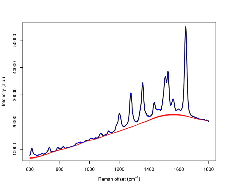
(a) Rhodamine B.

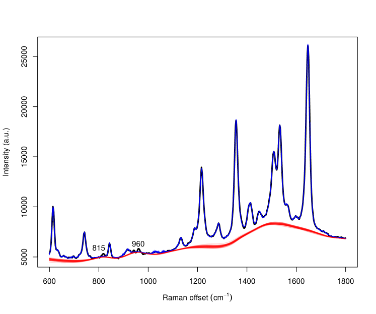
(b) TAMRA.

Figure 6: Posterior distributions for the peaks and baselines of rhodamine B and tetramethylrhodamine (TAMRA). Minor peaks at 815 and 960 cm^-1 have been missed by the model for TAMRA.

We used the 32 peak locations predicted by Watanabe et al. (2005) as an informative prior, as described in Sect. 3.1. Posterior distributions for rhodamine and TAMRA are illustrated in Fig. 6. 95% highest posterior density (HPD) intervals for the parameters of the peaks are provided in the supplementary material, as well as the results for eosin and FAM. Our SMC algorithm was able to match all of the observed peaks in the experimental spectra of rhodamine. Using the same prior, we also obtained a reasonably good fit for TAMRA. Only two minor peaks, at 815 and 960 cm^-1, were noticeably missing from the estimated spectral signature.

Table 1: 95% highest posterior density (HPD) intervals for the regression coefficients $\beta_{p}$ (inverse nanomolar, nM^-1), full width at half maximum (FWHM, cm^-1) and limit of detection (LOD, nM) of the 18 largest peaks in the TAMRA dilution study.

$\ell_{p}$ (cm-1)	$\beta_{p}$ (nM-1)	FWHM (cm-1)	LOD (nM)
460	[6.73; 17.23]	[0.00; 14.43]	[0.211; 0.784]
505	[167.95; 177.83]	[14.36; 15.52]	[0.019; 0.047]
632	[253.65; 263.16]	[11.54; 12.13]	[0.012; 0.032]
725	[19.63; 29.52]	[9.97; 16.43]	[0.123; 0.316]
752	[44.74; 54.81]	[19.49; 23.45]	[0.059; 0.156]
843	[23.48; 33.73]	[15.97; 22.26]	[0.106; 0.297]
965	[17.78; 28.09]	[12.07; 20.32]	[0.135; 0.355]
1140	[25.49; 36.11]	[20.41; 27.92]	[0.089; 0.253]
1190	[18.67; 28.99]	[11.27; 19.36]	[0.110; 0.352]
1220	[147.84; 158.30]	[17.68; 19.20]	[0.020; 0.051]
1290	[31.19; 42.49]	[15.72; 25.80]	[0.080; 0.213]
1358	[210.46; 221.96]	[17.63; 18.97]	[0.015; 0.035]
1422	[53.13; 63.99]	[15.34; 18.16]	[0.059; 0.135]
1455	[39.05; 53.87]	[20.61; 41.11]	[0.069; 0.175]
1512	[146.07; 157.28]	[20.81; 22.38]	[0.019; 0.049]
1536	[209.18; 221.03]	[14.43; 15.80]	[0.014; 0.036]
1570	[38.54; 53.67]	[23.87; 51.02]	[0.073; 0.173]
1655	[467.58; 477.91]	[17.40; 17.92]	[0.006; 0.016]

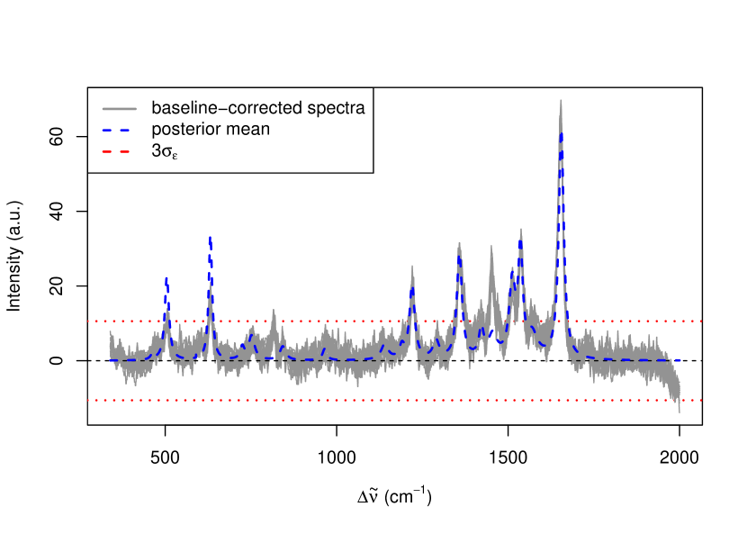
(a) TAMRA at 0.13 nM.

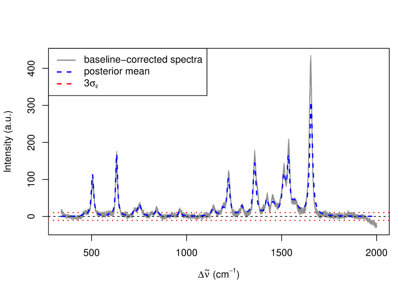
(b) TAMRA at 0.65 nM.

Figure 7: Observed spectra and model fit at very low dye concentrations.

Next, we used the IBIS algorithm (Chopin, 2002) to fit our model to the dilution study. 95% HPD intervals for the regression coefficients $\beta_{p}$, the FWHM and the LOD of the 18 largest peaks are shown in Table 1. To verify the HPD intervals for the LOD, we can closely examine the spectra at the two lowest concentrations, 0.13 and 0.65 nM. The lower bounds for detectability of the peaks at 460 and 965 cm^-1 are greater than 0.13 nM, so we would not expect those peaks to be visible at that concentration. Conversely, the upper bounds for 7 of the peaks are lower than 0.13 nM, so we would expect all of those peaks to be clearly visible, as shown by Fig. 7a. There is also an eighth peak at 1455 cm^-1 that has been underestimated by the model. The upper bounds for all of the peaks except at 460 cm^-1 are lower than 0.65 nM, so at least 17 out of 34 peaks should be visible at that concentration, as shown in Fig 7b. Care must be taken when extrapolating beyond the range of the data, but we predict that overall the LOD for TAMRA is between 6 and 16 picomolar (pM).

6 Discussion

This paper has employed statistical methods to advance both the theory and practice of Raman spectroscopy. We have been able to reconcile computational predictions of Raman peaks with experimental observations. Watanabe et al. (2005) used time-dependent density field theory (TD-DFT) to predict the peak locations of rhodamine. We derived an informative prior from these predictions and used an SMC algorithm to fit our model to observed spectra. This creates the potential to improve the quantum mechanical models that are used in computational chemistry by characterising the prediction error. For example, by performing calibration and emulation of the computational models (Kennedy and O’Hagan, 2001). Li et al. (2015) have already made some progress applying Bayesian emulation to molecular models.

On the more practical side, we have introduced a scalable algorithm for multivariate calibration (MVC). Our model-based approach provides several advantages over existing quantitative methods, such as univariate calibration or direct classical least squares (DCLS). We have represented the broadening of the Raman peaks using pseudo-Voigt functions, as in Ritter (1994); Frøhling et al. (2016). Unlike those previous papers, we also include a flexible model of the baseline, using a penalised B-spline. Our model has enabled us to directly estimate quantities of scientific interest, such as the amplitudes, limit of detection (LOD), and full width at half maximum (FWHM) of the Raman peaks. We have implemented our algorithm as an open source R package. This represents an important tool for analysing experimental data.

Our model could be extended to perform detection and quantification of multiplexed spectra, where several dye molecules may be present. Such a model would need to account for nonlinear interactions between molecules, for example due to preferential attachment (Gracie et al., 2016). Estimating the LOD for each peak would be particularly useful in this setting, since many of the peaks of different molecules overlap with each other. Such estimates could be used in experimental design, to select molecules that maximise differentiation between their spectral signatures. It would also be useful to extend our model to include spatial correlation between spectra. Some spectrometers are able to collect measurements on a 2D or 3D lattice, known as a Raman map. A divide-and-conquer SMC approach (Lindsten et al., 2017) could be applied in this setting, by dividing the hyperspectral data cube into sub-lattices.

References

- AIST (2001) AIST (2001). Spectral database for organic compounds (SDBS). National Institute of Advanced Industrial Science and Technology, Tokyo, Japan.
- Bell et al. (1998) Bell, I. M., R. J. H. Clark, and P. J. Gibbs (1998). Raman spectroscopic library of natural and synthetic pigments. University College London, UK.
- Boelens et al. (2005) Boelens, H. F. M., P. H. C. Eilers, and T. Hankemeier (2005). Sign constraints improve the detection of differences between complex spectral data sets: LC-IR as an example. Anal. Chem. 77(24), 7998–8007.
- Boyaci et al. (2012) Boyaci, I. H., H. E. Genis, B. Guven, U. Tamer, and N. Alper (2012). A novel method for quantification of ethanol and methanol in distilled alcoholic beverages using Raman spectroscopy. J. Raman Spectrosc. 43(8), 1171–1176.
- Butler et al. (2016) Butler, H. J., L. Ashton, B. Bird, G. Cinque, K. Curtis, J. Dorney, K. Esmonde-White, N. J. Fullwood, B. Gardner, P. L. Martin-Hirsch, M. J. Walsh, M. R. McAinsh, N. Stone, and F. L. Martin (2016). Using Raman spectroscopy to characterize biological materials. Nat. Protocols 11(4), 664–687.
- Cai et al. (2001) Cai, T. T., D. Zhang, and D. Ben-Amotz (2001). Enhanced chemical classification of Raman images using multiresolution wavelet transformation. Appl. Spectrosc. 55(9), 1124–30.
- Chib (1993) Chib, S. (1993). Bayes regression with autoregressive errors: A Gibbs sampling approach. J. Econometrics 58(3), 275–294.
- Chopin (2002) Chopin, N. (2002). A sequential particle filter method for static models. Biometrika 89(3), 539–551.
- Cressie and Johannesson (2008) Cressie, N. and G. Johannesson (2008). Fixed rank kriging for very large spatial data sets. J. R. Stat. Soc. Ser. B 70(1), 209–226.
- Datta et al. (2016) Datta, A., S. Banerjee, A. O. Finley, and A. E. Gelfand (2016). Hierarchical nearest-neighbor Gaussian process models for large geostatistical datasets. J. Am. Stat. Assoc.. In press.
- De Rooi and Eilers (2012) De Rooi, J. J. and P. H. C. Eilers (2012). Mixture models for baseline estimation. Chemometr. Intell. Lab. 117, 56–60.
- Del Moral et al. (2006) Del Moral, P., A. Doucet, and A. Jasra (2006). Sequential Monte Carlo samplers. J. R. Stat. Soc. Ser. B 68(3), 411–436.
- Douc et al. (2005) Douc, R., O. Cappé, and É. Moulines (2005). Comparison of resampling schemes for particle filtering. In Proc. 4th Int. Symp. Image and Signal Processing and Analysis (ISPA), Zagreb, Croatia, pp. 64–69. IEEE.
- Eilers and Marx (1996) Eilers, P. H. C. and B. D. Marx (1996). Flexible smoothing with B-splines and penalties. Statist. Sci. 11(2), 89–121.
- Ellis et al. (2013) Ellis, D. I., D. P. Cowcher, L. Ashton, S. O’Hagan, and R. Goodacre (2013). Illuminating disease and enlightening biomedicine: Raman spectroscopy as a diagnostic tool. Analyst 138, 3871–84.
- Ellis et al. (2017) Ellis, D. I., R. Eccles, Y. Xu, J. Griffen, H. Muhamadali, P. Matousek, I. Goodall, and R. Goodacre (2017). Through-container, extremely low concentration detection of multiple chemical markers of counterfeit alcohol using a handheld SORS device. Sci. Rep. 7(1), 12082.
- Eubank (1999) Eubank, R. L. (1999). Nonparametric Regression and Spline Smoothing (2nd ed.), Volume 157 of Statistics: textbooks and monographs. New York, NY: Marcel Dekker.
- Fischer and Dose (2002) Fischer, R. and V. Dose (2002). Physical mixture modeling with unknown number of components. In Proc. 21st Int. Wkshp MaxEnt, Volume 617 of AIP Conf. Proc., pp. 143–154.
- Frøhling et al. (2016) Frøhling, K. B., T. S. Alstrøm, M. Bache, M. S. Schmidt, M. N. Schmidt, J. Larsen, M. H. Jakobsen, and A. Boisen (2016). Surface-enhanced Raman spectroscopic study of DNA and 6-mercapto-1-hexanol interactions using large area mapping. Vib. Spectrosc. 86, 331–336.
- Galloway et al. (2009) Galloway, C. M., E. C. Le Ru, and P. G. Etchegoin (2009). An iterative algorithm for background removal in spectroscopy by wavelet transforms. Appl. Spectrosc. 63(12), 1370–1376.
- Gan et al. (2006) Gan, F., G. Ruan, and J. Mo (2006). Baseline correction by improved iterative polynomial fitting with automatic threshold. Chemometr. Intell. Lab. 82(1–2), 59–65.
- Gracie et al. (2014) Gracie, K., E. Correa, S. Mabbott, J. A. Dougan, D. Graham, R. Goodacre, and K. Faulds (2014). Simultaneous detection and quantification of three bacterial meningitis pathogens by SERS. Chem. Sci. 5, 1030–40.
- Gracie et al. (2016) Gracie, K., M. Moores, W. E. Smith, K. Harding, M. Girolami, D. Graham, and K. Faulds (2016). Preferential attachment of specific fluorescent dyes and dye labelled DNA sequences in a SERS multiplex. Anal. Chem. 88(2), 1147–1153.
- Green (1995) Green, P. J. (1995). Reversible jump Markov chain Monte Carlo computation and Bayesian model determination. Biometrika 82(4), 711–732.
- Green and Silverman (1994) Green, P. J. and B. W. Silverman (1994). Nonparametric regression and generalized linear models: a roughness penalty approach, Volume 58 of Monographs on Statistics and Applied Probability. Boca Raton, FL: Chapman & Hall/CRC Press.
- Greeneltch et al. (2012) Greeneltch, N. G., A. S. Davis, N. A. Valley, F. Casadio, G. C. Schatz, R. P. Van Duyne, and N. C. Shah (2012). Near-infrared surface-enhanced Raman spectroscopy (NIR-SERS) for the identification of eosin Y: Theoretical calculations and evaluation of two different nanoplasmonic substrates. J. Phys. Chem. A 116(48), 11863–11869.
- Haaland and Easterling (1980) Haaland, D. M. and R. G. Easterling (1980). Improved sensitivity of infrared spectroscopy by the application of least squares methods. Appl. Spectrosc. 34(5), 539–548.
- He et al. (2014) He, S., W. Zhang, L. Liu, Y. Huang, J. He, W. Xie, P. Wu, and C. Du (2014). Baseline correction for Raman spectra using an improved asymmetric least squares method. Anal. Methods 6(12), 4402–4407.
- Ida et al. (2000) Ida, T., M. Ando, and H. Toraya (2000). Extended pseudo-Voigt function for approximating the Voigt profile. J. Appl. Crystallogr. 33(6), 1311–1316.
- Jensen et al. (2008) Jensen, L., C. M. Aikens, and G. C. Schatz (2008). Electronic structure methods for studying surface-enhanced Raman scattering. Chem. Soc. Rev. 37, 1061–1073.
- Jones et al. (1999) Jones, J. C., C. McLaughlin, D. Littlejohn, D. A. Sadler, D. Graham, and W. E. Smith (1999). Quantitative assessment of surface-enhanced resonance Raman scattering for the analysis of dyes on colloidal silver. Anal. Chem. 71(3), 596–601.
- Kearns et al. (2016) Kearns, H., S. Sengupta, I. Ramos Sasselli, L. Bromley III, K. Faulds, T. Tuttle, M. A. Bedics, M. R. Detty, L. Velarde, D. Graham, and W. E. Smith (2016). Elucidation of the bonding of a near infrared dye to hollow gold nanospheres – a chalcogen tripod. Chem. Sci.. In press.
- Kennedy and O’Hagan (2001) Kennedy, M. C. and A. O’Hagan (2001). Bayesian calibration of computer models. J. R. Stat. Soc. Ser. B 63(3), 425–464.
- Kleinman et al. (2011) Kleinman, S. L., E. Ringe, N. Valley, K. L. Wustholz, E. Phillips, K. A. Scheidt, G. C. Schatz, and R. P. V. Duyne (2011). Single-molecule surface-enhanced raman spectroscopy of crystal violet isotopologues: Theory and experiment. J. Am. Chem. Soc. 133(11), 4115–4122.
- Kong et al. (1994) Kong, A., J. S. Liu, and W. H. Wong (1994). Sequential imputations and Bayesian missing data problems. J. Am. Stat. Assoc. 89(425), 278–288.
- Lafuente et al. (2015) Lafuente, B., R. T. Downs, H. Yang, and N. Stone (2015). The power of databases: the RRUFF project. In T. Armbruster and R. M. Danisi (Eds.), Highlights in Mineralogical Crystallography, pp. 1–30. Berlin, Germany: W. De Gruyter.
- Laing et al. (2017) Laing, S., L. E. Jamieson, K. Faulds, and D. Graham (2017). Surface-enhanced Raman spectroscopy for in vivo biosensing. Nat. Rev. Chem. 1, 0060.
- Le Ru and Etchegoin (2009) Le Ru, E. C. and P. G. Etchegoin (2009). Principles of Surface-Enhanced Raman Spectroscopy and Related Plasmonic Effects. Amsterdam, Netherlands: Elsevier.
- Li et al. (2015) Li, Z., J. R. Kermode, and A. De Vita (2015). Molecular dynamics with on-the-fly machine learning of quantum-mechanical forces. Phys. Rev. Lett. 114, 096405.
- Lieber and Mahadevan-Jansen (2003) Lieber, C. A. and A. Mahadevan-Jansen (2003). Automated method for subtraction of fluorescence from biological Raman spectra. Appl. Spectrosc. 57(11), 1363–1367.
- Liland et al. (2010) Liland, K. H., T. Almøy, and B.-H. Mevik (2010). Optimal choice of baseline correction for multivariate calibration of spectra. Appl. Spectrosc. 64(9), 234A–268A.
- Lin-Vien et al. (1991) Lin-Vien, D., N. B. Colthup, W. G. Fateley, and J. G. Grasselli (1991). The Handbook of Infrared and Raman Characteristic Frequencies of Organic Molecules. San Diego, CA: Academic Press.
- Lindgren et al. (2011) Lindgren, F., H. Rue, and J. Lindström (2011). An explicit link between Gaussian fields and Gaussian Markov random fields: the stochastic partial differential equation approach. J. R. Stat. Soc. Ser. B 73(4), 423–498.
- Lindsten et al. (2017) Lindsten, F., A. M. Johansen, C. A. Næsseth, B. Kirkpatrick, T. B. Schön, J. A. D. Aston, and A. Bouchard-Côté (2017). Divide-and-conquer with sequential Monte Carlo. J. Comput. Graph. Stat. 26(2), 445–458.
- Liu (2001) Liu, J. S. (2001). Monte Carlo Strategies in Scientific Computing. Springer Series in Statistics. New York, NY: Springer.
- Liu and Chen (1998) Liu, J. S. and R. Chen (1998). Sequential Monte Carlo methods for dynamic systems. J. Am. Stat. Assoc. 93(443), 1032–1044.
- Mammone et al. (1980) Mammone, J. F., S. K. Sharma, and M. Nicol (1980). Raman spectra of methanol and ethanol at pressures up to 100 kbar. J. Phys. Chem. 84(23), 3130–3134.
- Murray et al. (2016) Murray, L. M., A. Lee, and P. E. Jacob (2016). Parallel resampling in the particle filter. J. Comput. Graph. Stat.. In press.
- Pelletier (2003) Pelletier, M. J. (2003). Quantitative analysis using Raman spectrometry. Appl. Spectrosc. 57(1), 20A–42A.
- R Core Team (2017) R Core Team (2017). R: A Language and Environment for Statistical Computing. Vienna, Austria: R Foundation for Statistical Computing.
- Ramsay and Silverman (2005) Ramsay, J. O. and B. W. Silverman (2005). Functional Data Analysis (2nd ed.). New York, NY: Springer.
- Rasmussen and Williams (2006) Rasmussen, C. E. and C. K. I. Williams (2006). Gaussian Processes for Machine Learning. Cambridge, MA: MIT Press.
- Razul et al. (2003) Razul, S. G., W. J. Fitzgerald, and C. Andrieu (2003). Bayesian model selection and parameter estimation of nuclear emission spectra using RJMCMC. Nucl. Instrum. Meth. A 497(2–3), 492–510.
- Ritter (1994) Ritter, C. (1994). Statistical analysis of spectra from electron spectroscopy for chemical analysis. J. R. Stat. Soc. Ser. D 43(1), 111–127.
- Ruckstuhl et al. (2001) Ruckstuhl, A. F., M. P. Jacobson, R. W. Field, and J. A. Dodd (2001). Baseline subtraction using robust local regression estimation. J. Quant. Spectrosc. Ra. 68(2), 179–193.
- Thompson et al. (1987) Thompson, P., D. E. Cox, and J. B. Hastings (1987). Rietveld refinement of Debye–Scherrer synchrotron X-ray data from Al2O3. J. Appl. Crystallogr. 20(2), 79–83.
- Van Caillie and Amos (2000) Van Caillie, C. and R. D. Amos (2000). Raman intensities using time dependent density functional theory. Phys. Chem. Chem. Phys. 2, 2123–29.
- van Dyk et al. (2001) van Dyk, D. A., A. Connors, V. L. Kashyap, and A. Siemiginowska (2001). Analysis of energy spectra with low photon counts via Bayesian posterior simulation. Astrophys. J. 548(1), 224–243.
- van Dyk and Kang (2004) van Dyk, D. A. and H. Kang (2004). Highly structured models for spectral analysis in high-energy astrophysics. Statist. Sci. 19(2), 275–293.
- Varmuza and Filzmoser (2009) Varmuza, K. and P. Filzmoser (2009). Introduction to Multivariate Statistical Analysis in Chemometrics. Boca Raton, FL: Chapman & Hall/CRC Press.
- Wang et al. (2008) Wang, Y., X. Zhou, H. Wang, K. Li, L. Yao, and S. T. C. Wong (2008). Reversible jump MCMC approach for peak identification for stroke SELDI mass spectrometry using mixture model. Bioinformatics 24(13), i407–i413.
- Watanabe et al. (2005) Watanabe, H., N. Hayazawa, Y. Inouye, and S. Kawata (2005). DFT vibrational calculations of rhodamine 6G adsorbed on silver: Analysis of tip-enhanced Raman spectroscopy. J. Phys. Chem. B 109(11), 5012–5020.
- Wertheim and Dicenzo (1985) Wertheim, G. K. and S. B. Dicenzo (1985). Least-squares analysis of photoemission data. J. Electron Spectrosc. Relat. Phenom. 37(1), 57–67.
- Zavaleta et al. (2009) Zavaleta, C. L., B. R. Smith, I. Walton, W. Doering, G. Davis, B. Shojaei, M. J. Natan, and S. S. Gambhir (2009). Multiplexed imaging of surface enhanced Raman scattering nanotags in living mice using noninvasive Raman spectroscopy. Proc. Natl Acad. Sci. USA 106(32), 13511–13516.
- Zhong et al. (2011) Zhong, M., M. Girolami, K. Faulds, and D. Graham (2011). Bayesian methods to detect dye-labelled DNA oligonucleotides in multiplexed Raman spectra. J. R. Stat. Soc. Ser. C 60(2), 187–206.