Cosmic Infrared Background Fluctuations and Zodiacal Light

Abstract

We have performed a specific observational test to measure the effect that the zodiacal light can have on measurements of the spatial fluctuations of the near-IR background. Previous estimates of possible fluctuations caused by zodiacal light have often been extrapolated from observations of the thermal emission at longer wavelengths and low angular resolution, or from IRAC observations of high latitude fields where zodiacal light is faint and not strongly varying with time. The new observations analyzed here target the COSMOS field, at low ecliptic latitude where the zodiacal light intensity varies by factors of $\sim 2$ over the range of solar elongations at which the field can be observed. We find that the white noise component of the spatial power spectrum of the background is correlated with the modeled zodiacal light intensity. At large angular scales ($\gtrsim 100^{\prime\prime}$) where excess power above the white noise is observed, we find no correlation of the power with the modeled intensity of the zodiacal light. This test clearly indicates that the large scale power in the infrared background is not being caused by the zodiacal light.

1 Introduction

The study of astronomical backgrounds at various wavelengths allows the examination of sources that are intrinsically diffuse, or individually too faint or too confused to be detected. Over time, improvements in instrumentation may resolve increasingly fainter sources, but very faint and intrinsically diffuse sources always remain in the realm of background studies.

Studies of the cosmic infrared background (CIB) have aimed at measuring the cumulative stellar emission of galaxies across entire history of the universe. Measurements made by the DIRBE instrument on COBE provided the first space-based measurements of the absolute sky surface brightness at wavelengths from 1.25 to 240 $\mu$m with an angular resolution of $0\fdg 7$ (Hauser et al., 1998). However, difficulties in accurately removing foreground contributions from the zodiacal light (Kelsall et al., 1998), and from Galactic stars and interstellar dust (Arendt et al., 1998) prevented precise detections of the CIB except at the longest wavelengths.

Subsequent measurements and studies of the CIB at near- to mid-IR wavelengths have made use of telescopes and instruments that provide much higher angular resolution than DIRBE, but which usually cover only a small fraction of the sky, e.g. 2MASS, Spitzer, HST, IRTS, AKARI, CIBER. The higher angular resolution allows the exclusion or subtraction of stars and bright galaxies from sky brightness measurements, such that the contribution of Galactic stars is minimized, and the CIB that remains does not include the contributions of galaxies brighter than certain limits dependent on depth of the observations. These data sets are often better suited for measuring the spatial fluctuations or structure of the “source-subtracted” CIB, rather than for measuring the mean value of the CIB (Kashlinsky et al., 1996a, b, 2002, 2005, 2007, 2012; Kashlinsky & Odenwald, 2000; Odenwald et al., 2003; Matsumoto et al., 2005, 2015, 2011; Thompson et al., 2007a, b; Cooray et al., 2007; Sullivan et al., 2007; Arendt et al., 2010; Matsuura et al., 2011; Pyo et al., 2012; Zemcov et al., 2014; Donnerstein, 2015; Mitchell-Wynne et al., 2015; Seo et al., 2015). These studies seem to show reasonable consistency of fluctuation measurements reported by different experiments and different groups at $\lambda\gtrsim 2$ $\mu$m, though the picture is less clear at shorter wavelengths.

The of the fluctuations is not yet clear. The fluctuations may arise from any or all of: solar system and Galactic foregrounds, nearby extragalactic contributions, and distant extragalactic contributions. In most cases (e.g. Kashlinsky et al., 2005; Arendt et al., 2010; Matsumoto et al., 2011; Zemcov et al., 2014) foregrounds are estimated by extrapolation of measurements at other wavelengths and locations. This is particularly true of zodiacal light contributions. Mid-IR observations using ISO have limited zodiacal light fluctuations to $<0.2\%$ on scales $>3^{\prime}$ (Abraham et al., 1997). More recent AKARI measurement set the limit even lower at $0.03\%$ (Pyo et al., 2012).

Direct detection of zodiacal light influences in Spitzer IRAC measurements have been checked in existing deep data sets by constructing $A-B$ difference maps, where $A$ and $B$ represent observations made at two different epochs, typically 6 months and/or 1 year apart (e.g. Kashlinsky et al., 2007). The expectation is that the first-order gradient should reverse at 6-month intervals, while any smaller scale, physically distinct structures in the interplanetary dust cloud should not remain fixed in a given field (due to differential rotation of the cloud) and should not appear the same at different epochs separated by 6 months. Excess differences have not been seen in existing deep CIB studies. However, these are generally high latitude fields where the zodiacal light is faint and not strongly modulated. Additionally, at intervals of 6 months and (especially) 1 year, the interplanetary dust cloud may be sufficiently symmetric such that certain structures (e.g. those associated with the earth-resonant ring) may still cancel out in $A-B$ difference maps.

As a more certain test for zodiacal light influences, our new Spitzer IRAC observations have monitored a low latitude field over an entire visibility window to obtain a data set where the zodiacal light is both brightest and most strongly modulated. The observations were planned to be sufficiently deep to detect the reported large scale background structure. Thus these data are uniquely suitable for checking if the zodiacal light intensity has any effect on the reported background fluctuations at large angular scales.

This paper reports on this test and the results. The observations and data reduction are described in sections 2 and 3. Section 4 provides the characterization of the power spectra of the background. Section 5 discusses the correlations between the various components of the power spectrum and the zodiacal light intensity. Section 6 summarizes the results. An appendix provides additional detail on temporal variations in the data that are tracked and corrected by the self-calibration procedure that we apply. The appendix also features additional details on the effects of the source model, and on the comparison with previous CIB measurements.

2 Observations

Most commonly observed extragalactic fields are chosen to be at high Galactic and ecliptic latitudes to minimize the influence of foregrounds. The COSMOS field (Scoville et al., 2007; Ashby et al., 2013, 2015) is suitable for our experiment, as it lies at relatively low ecliptic latitude. We have selected a subregion at ecliptic coordinates $(\lambda,\beta)=(151.73,-8.63)$ which is relatively free of bright sources. The patch is observed 5 times across an entire visibility window of the Spitzer spacecraft (Werner et al., 2004; Gehrz et al., 2007), covering the widest possible range of solar elongation, and thus brightness. The size, $\sim 10^{\prime}\times 10^{\prime}$, and depth, $\sim 4$ hr per epoch, of the patch were chosen to be sufficiently wide and deep to distinguish the large scale fluctuations above the random white noise in the observations. We use Spitzer’s IRAC instrument (Fazio et al., 2004) to collect 3.6 and 4.5 $\mu$m data. As IRAC’s field of view is $5^{\prime}\times 5^{\prime}$, the observations require mosaicking $2\times 2$ fields of view and a total observing time of $\sim 16$ hr at each epoch. Table 1 lists the dates, solar elongations, and astronomical observation request (AOR) numbers of the observations.

Table 1: COSMOS Zodiacal Light Observations

Epoch	Date	MJD	AOR	Solar Elongation
1	2013 Jan 26	56318.111	42306048	000083.6
2	2013 Feb 02	56325.130	42306304	90.3
3	2013 Feb 13	56336.289	42306560	101.0
4	2013 Feb 24	56347.142	42306816	111.5
5	2013 Mar 02	56353.211	42307072	117.3

Note. — MJD = modified julian date, AOR = astronomical observation request; Program ID = 80062

3 Data Reduction

3.1 Self-Calibration

We reduce the data using the same self-calibration techniques (Fixsen et al., 2000) that have been previously employed (Arendt et al., 2010). The data reduction began with the IRAC cBCD individual frames and applied a data model of

$$D^{i}=S^{\alpha}+F^{p}+F^{q}$$ (1)

where $D^{i}$ is the measured intensity at pixel $i$ in a single frame ($q$), $S^{\alpha}$ is the true sky intensity at location $\alpha$, $F^{p}$ is an offset for pixel $i$ which is constant over all frames, and $F^{q}$ is an offset for frame $q$ which is constant over all pixels (but variable with time). Each of the 5 epochs is self-calibrated separately to provide detector offsets, $F^{p}$, that are appropriate for each epoch. Sky maps are generated on a pixel scale of $0.6^{\prime\prime}$ (half the size of the detector pixels) using an interlacing algorithm. In addition to regular sky maps, we also create $A-B$ sky maps where all the odd numbered frames are multiplied by $-1$ before mosaicking the image. This has the effect of removing the contributions of fixed celestial sources and leaving only instrumental noise (and photon shot noise, see Section 4.1).

Figure 1: Only the two brightest stars in the 3.6 $\mu$m image show a small residual of incompletely corrected “column pull-down” artifacts (dark vertical stripes). The images are logarithmically scaled on the range [$2.5\times 10^{-4}$, 1.0] MJy sr^-1 after addition of an offset of 0.004 MJy sr^-1 to avoid logarithmic scaling of negative data values. The images are 900$\times$900 pixels or $9^{\prime}\times 9^{\prime}$ in size (1 pixel = $0.6^{\prime\prime}$). Celestial north is at a position angle of $66\fdg 4$ (counterclockwise from vertical). There is only $\sim 25\%$ overlap between the fields.

Figure 1 shows the 3.6 and 4.5 $\micron$ images ($S^{\alpha}$ determined by self-calibration) of the combined 5 epochs of observations. The images are cropped to show only the roughly uniformly covered region that was used for power spectrum analysis. Linear background gradients have been fitted and subtracted.

Figure 2 displays the derived values of the detector offsets, $F^{p}$, for 3.6 and 4.5 $\mu$m at all 5 epochs. At all epochs there are different patterns of light and dark latent images, which are very slowly decaying imprints of very bright stars as they were dithered across the detector in previous observations. In several cases the tracks of bright stars that slewed across the detector between pointings can also be seen. Residual stray light in the cBCD frames is also revealed and removed by the self-calibration. Diffuse patches of stray light are created by the zodiacal light (and the sum of all other backgrounds) in the upper left and upper right corners of both the 3.6 and 4.5 $\mu$m detectors. The BCD pipeline uses estimates of the expected brightness of the zodiacal light to model and remove this stray light component. These self-calibration results show that at 3.6 $\mu$m that process works well initially, when the zodiacal light is bright, but has an increasing error at later epochs as the elongation increases and the zodiacal light becomes fainter. The opposite occurs at 4.5 $\mu$m, where the standard correction works best at the later high-elongation epochs and less well at the early epochs when the zodiacal light is brighter. All these features visible in the $F^{p}$ maps are systematic effects that are removed by the self-calibration of the data.

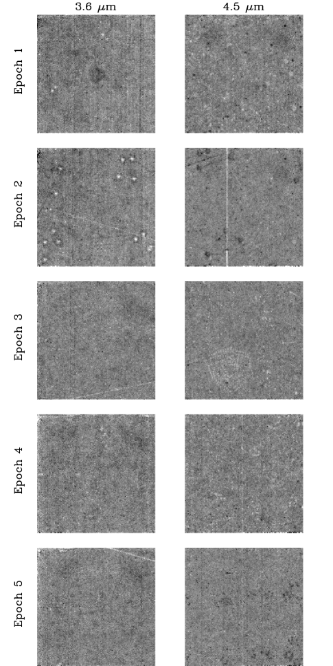
Figure 2: Maps of the self-calibration $F^{p}$ offsets derived for each epoch. Different long-term latent images are present at each epoch. The effects of residual straylight in the cBCD images are evident as diffuse dark patches in the upper left and right corners of the later epochs at 3.6 $\micron$ and the early epochs at 4.5 $\micron$. All images are on a linear stretch of [$-0.015$, $+0.015$] MJy sr^-1.

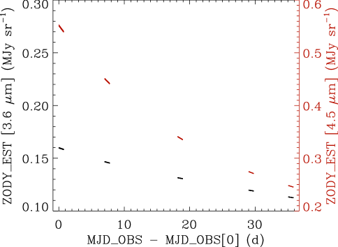
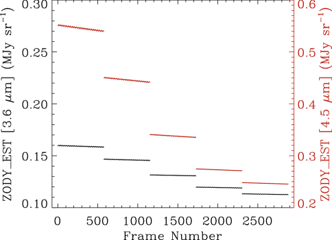
Figure 3: The predicted zodiacal light intensity as given by the ZODY_EST keyword in the cBCD frames. The top plot shows the steady decline in intensity as a function of time. The fractional decrease at 4.5 $\mu$m is larger than that at 3.6 $\mu$m. Plotting simply as a function of frame number (bottom) provides a slightly clearer look at the very small oscillations in intensity that are caused by moving up and down the zodiacal light gradient at different pointings.

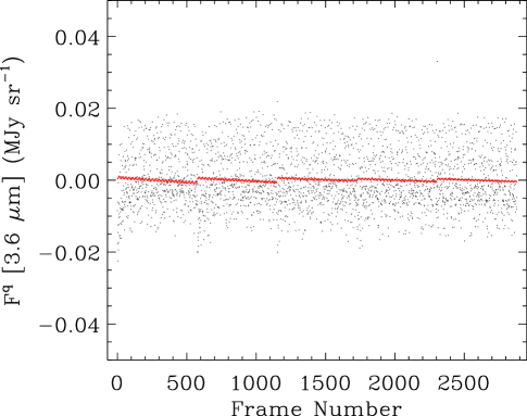
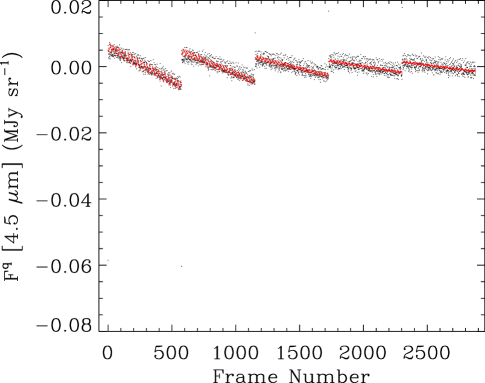
Figure 4: Comparison between the self-calibration $F^{q}$ offsets (black dots) and the ZODY_EST keyword values (red dots) after subtraction of the mean values for each epoch. The lack of perfect correlation between these reflects errors in the zodiacal light model and the presence of additional temporally variable effects in the data , which are removed by $F^{q}$.

Figure 3 shows expected general trend of the zodiacal light intensity as a function of time, as estimated by the Spitzer foreground model and given as the ZODY_EST keyword in the header of each frame. Note the 4.5 $\micron$ intensity is a stronger function of time or elongation than the 3.6 $\micron$ intensity, indicating that the color of the zodiacal light is not expected to be constant. The self-calibration model applied in Equation (1) assumes a fixed sky intensity. Thus any variations in brightness due to changing zodiacal light intensity across the span of the data being self-calibrated, or a single epoch, are absorbed by the variable offset term, $F^{q}$. Figure 4 shows that $F^{q}$ varies by a much larger amount than the expected zodiacal light trends at 3.6 $\mu$m, but is similar to the expected zodiacal light trends at 4.5 $\mu$m. In the Appendix we show that the differences are real and represent corrections for transient instrumental effects (not fully corrected in the BCD pipeline), and residual linear gradients across the field.

3.2 Source Subtraction and Masking

For measurement of the power spectra of the background, resolved sources need to be masked or modeled and subtracted from the images. As in prior studies, we subtract the flux from sources above the noise level using an iterative algorithm described by Arendt et al. (2010). The iterations are halted when the skewness of the intensity distribution of the remaining pixels is zero (independently for each epoch). Because the removal is imperfect, the image is also masked using a mask derived from a surface brightness threshold in the original images for all epochs combined. The masking threshold can equivalently be expressed as a specified surface brightness, a specified maximum outlier in the distribution of surface brightness of unmasked pixels, or a specified fraction of area masked. In this case we chose the last constraint, limiting the masked out regions at both wavelengths to 25% of the image, leaving 75% of the image remaining. At 3.6 and 4.5 $\mu$m, this limit corresponds surface brightness thresholds of ${\rm max}(I_{\nu})-{\rm mean}(I_{\nu})=0.0057$ and 0.0044 MJy sr^-1, and to maximum outliers of ${\rm max}(I_{\nu})/\sigma_{I_{\nu}}=3.2$ and 2.6 respectively.

4 Power Spectra

The power spectra of the source-subtracted images are calculated as described by Arendt et al. (2010). The power on the horizontal ($u=0$) and vertical ($v=0$) axes in the Fourier domain is omitted when averaging the power in bins at different angular scales, $2\pi/q$. This makes the results less susceptible to certain systematic errors (such as the residual column pull-down seen at 3.6 $\mu$m in Figure 1), but limits the maximum angular scale to $382^{\prime\prime}=540^{\prime\prime}/\sqrt{2}$ instead of the full $540^{\prime\prime}$ size of the field. The resulting power spectra, for the five epochs combined, and for each epoch individually are plotted in Figures 5 and 6.

The power spectra are characterized as in Arendt et al. (2010) by fitting a combination of 3 simple components:

$$P(q)=a_{0}(2\pi/q/100^{\prime\prime})^{a_{1}}\ P_{\rm PRF}(q)+a_{2}\ P_{\rm PRF}(q)+a_{3}$$ (2)

where the parameters $a_{0}$ and $a_{1}$ are the amplitude and index of a power-law component that is modulated by the instrument beam or point response function, $P_{\rm PRF}(q)$, the parameter $a_{2}$ is the amplitude of the sky shot noise: a white shot-noise component that is also modulated by the beam (e.g. Poisson variation in the number of faint unresolvable sources in the beam at each location), and $a_{3}$ is the amplitude of a white (shot noise) component that is not modulated by the beam. As an alternate characterization, we also fit:

$$P(q)=b_{0}(2\pi/q/100^{\prime\prime})^{b_{1}}\ P_{\rm PRF}(q)+b_{2}\ P_{\rm PRF}(q)+P_{A-B}(q)$$ (3)

where the white noise component is replaced by the measured $A-B$ power spectrum with no rescaling allowed. These characterizations of the power spectra are overplotted in Figures 5 and 6 and are tabulated in Table 2.

We note that one could apply a more physical model for characterization of the large-scale component of the power spectra, e.g. a $\Lambda$CDM template. However, a simple power law provides a sufficient approximation for a wide possibility of origins, given the angular scales ($\lesssim 400^{\prime\prime}$) and quality of the data analyzed here.

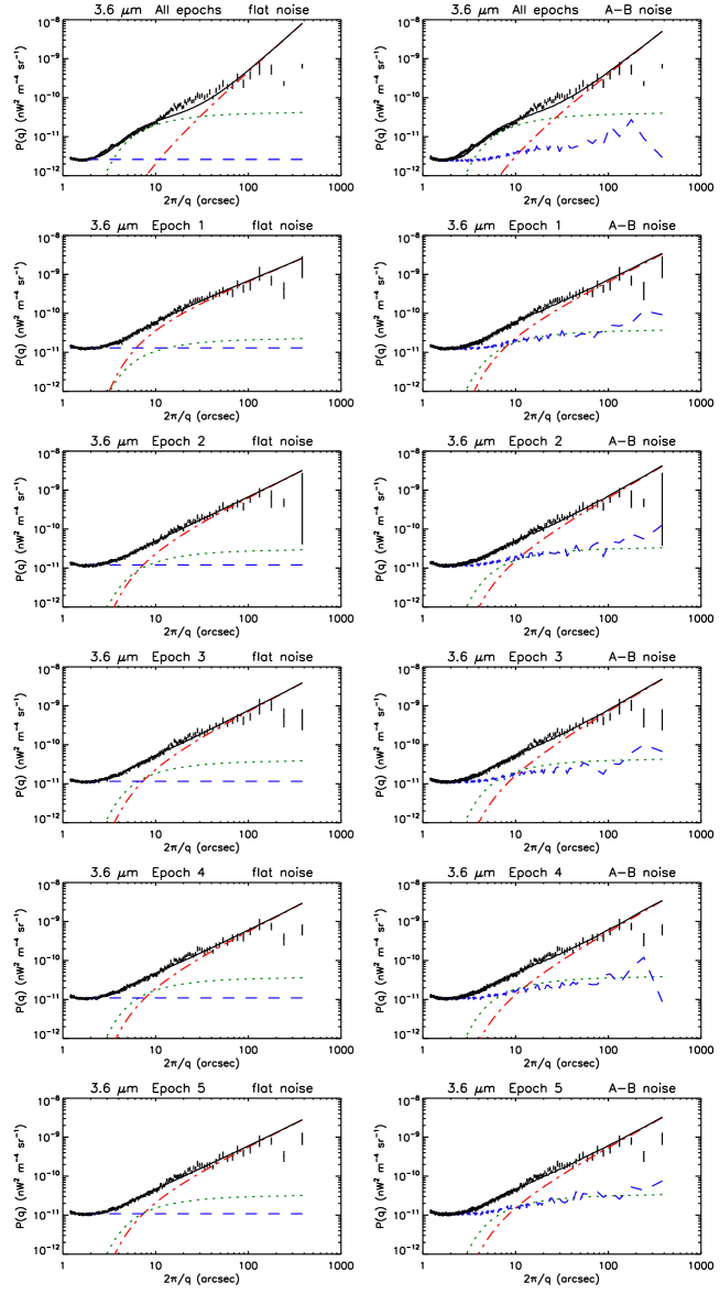
Figure 5: Fits to the 3.6 $\micron$ power spectra for all epochs combined, and for each of the 5 separate epochs. The left column shows fits as characterized by Equation (2): The right column shows the fits as characterized by Equation (3), where the measured (A-B)/2 noise takes the place of the flat instrument noise component.

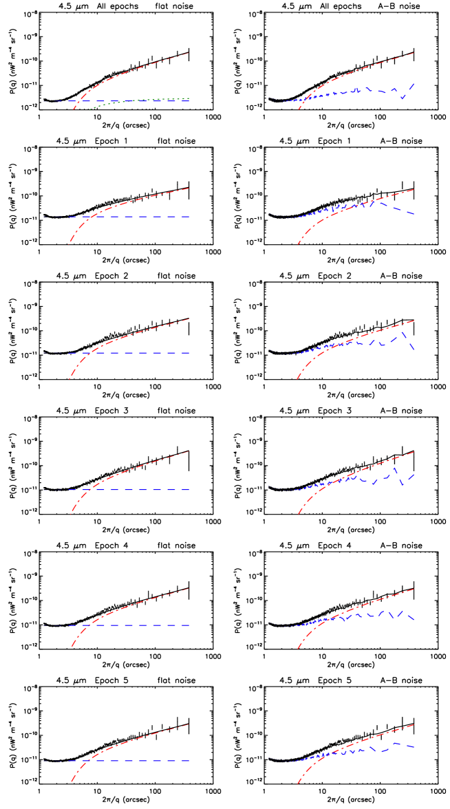
Figure 6: Same as Fig. 5, except for 4.5 $\micron$.

Table 2: Power Spectrum Parameters

$\lambda$ ($\micron$)	Epoch	$10^{11}a_{0}$		$a_{1}$		$10^{11}a_{2}$		$10^{11}a_{3}$		$\chi^{2}_{\nu}$	$10^{11}b_{0}$	$b_{1}$	$10^{11}b_{2}$	$\chi^{2}_{\nu}$
3.6	All epochs	50.24$\pm$ 2	2.07$\pm$ 0.06	4.19$\pm$ 0	0.26$\pm$ 0.001	4.47	43.76$\pm$ 2.90	1.82$\pm$ 0	4.01$\pm$ 0.05	5.92
3.6	Epoch 1	70.58$\pm$ 4	0.97$\pm$ 0.05	2.26$\pm$ 0	1.30$\pm$ 0.003	2.73	70.28$\pm$ 4.65	1.16$\pm$ 0	3.73$\pm$ 0.28	2.48
3.6	Epoch 2	68.39$\pm$ 4	1.15$\pm$ 0.05	2.95$\pm$ 0	1.20$\pm$ 0.002	2.99	68.90$\pm$ 4.60	1.33$\pm$ 0	3.33$\pm$ 0.20	2.76
3.6	Epoch 3	77.19$\pm$ 4	1.20$\pm$ 0.05	3.89$\pm$ 0	1.16$\pm$ 0.002	2.44	77.67$\pm$ 5.09	1.35$\pm$ 0	4.26$\pm$ 0.20	2.90
3.6	Epoch 4	60.29$\pm$ 3	1.18$\pm$ 0.05	3.63$\pm$ 0	1.09$\pm$ 0.002	2.67	58.09$\pm$ 3.75	1.32$\pm$ 0	3.86$\pm$ 0.18	2.52
3.6	Epoch 5	60.30$\pm$ 3	1.14$\pm$ 0.05	3.20$\pm$ 0	1.09$\pm$ 0.002	2.54	58.36$\pm$ 3.82	1.26$\pm$ 0	3.36$\pm$ 0.20	3.38
4.5	All epochs	9.61$\pm$ 0	0.65$\pm$ 0.02	0.29$\pm$ 0	0.23$\pm$ 0.001	3.55	9.44$\pm$ 0.20	0.65$\pm$ 0	0.06$\pm$ 0.11	7.25
4.5	Epoch 1	11.59$\pm$ 0	0.46$\pm$ 0.04	0.00$\pm$ 0	1.39$\pm$ 0.003	5.21	8.50$\pm$ 0.52	0.59$\pm$ 0	0.00$\pm$ 0.40	4.56
4.5	Epoch 2	14.94$\pm$ 0	0.56$\pm$ 0.03	0.00$\pm$ 0	1.21$\pm$ 0.003	5.15	11.38$\pm$ 0.53	0.63$\pm$ 0	0.00$\pm$ 0.31	4.51
4.5	Epoch 3	16.76$\pm$ 0	0.66$\pm$ 0.03	0.00$\pm$ 0	1.05$\pm$ 0.002	4.27	13.62$\pm$ 0.41	0.75$\pm$ 0	0.00$\pm$ 0.22	4.24
4.5	Epoch 4	14.37$\pm$ 0	0.61$\pm$ 0.03	0.00$\pm$ 0	0.95$\pm$ 0.002	4.11	12.11$\pm$ 0.37	0.68$\pm$ 0	0.00$\pm$ 0.25	3.57
4.5	Epoch 5	13.52$\pm$ 0	0.58$\pm$ 0.03	0.00$\pm$ 0	0.91$\pm$ 0.002	3.81	11.36$\pm$ 0.38	0.66$\pm$ 0	0.00$\pm$ 0.26	4.29
4.5	All epochs	8.34$\pm$ 0	1.0	1.35$\pm$ 0	0.23$\pm$ 0.000	3.93	8.15$\pm$ 0.17	1.0	1.09$\pm$ 0.02	7.91
4.5	Epoch 1	7.46$\pm$ 0	1.0	2.88$\pm$ 0	1.38$\pm$ 0.003	6.03	6.46$\pm$ 0.21	1.0	1.29$\pm$ 0.07	4.81
4.5	Epoch 2	9.22$\pm$ 0	1.0	2.57$\pm$ 0	1.20$\pm$ 0.002	6.30	7.76$\pm$ 0.24	1.0	1.44$\pm$ 0.07	5.00
4.5	Epoch 3	14.32$\pm$ 0	1.0	1.81$\pm$ 0	1.04$\pm$ 0.002	4.92	12.24$\pm$ 0.32	1.0	0.87$\pm$ 0.06	4.47
4.5	Epoch 4	12.02$\pm$ 0	1.0	1.92$\pm$ 0	0.94$\pm$ 0.002	4.82	10.51$\pm$ 0.25	1.0	1.18$\pm$ 0.05	3.91
4.5	Epoch 5	11.09$\pm$ 0	1.0	1.99$\pm$ 0	0.90$\pm$ 0.002	4.62	9.84$\pm$ 0.26	1.0	1.17$\pm$ 0.05	4.75

Note. — Units for $a_{0}$, $a_{2}$, $a_{3}$, $b_{0}$, and $b_{2}$ are nW² m^-4 sr^-1.

4.1 White Noise Component

The white noise component of the power spectrum, $a_{3}$ in Equation (2), includes instrumental noise, but it also includes the photon shot noise from celestial sources. In particular, the zodiacal light is the dominant brightness component. Because it is an approximately uniform source of emission, the power spectrum of its photon shot noise is not modulated by the beam. As a noise term it also does not cancel out in the construction of the $A-B$ difference images, and therefore the power spectra of those images also include the photon shot noise of the zodiacal

slight rise in the white noise component at the smallest angular scales an artifact of mapping data, sampled on $1\farcs 2$ detector pixels, onto a parallel sky map with $0\farcs 6$ pixels. For example, if the sky map is generated on grid that is rotated by $45\arcdeg$ to the detector orientation, then the white noise component does appear flat.

Figure 7 shows the very strong correlation between the zodiacal light intensity and the measured level of the white noise power spectrum. Extrapolation to zero intensity of the zodiacal light indicates that white noise power levels in the absence of zodiacal light would be $\times 10^{-12}$ and $\times 10^{-12}$ nW² m^-4 sr^-1 at 3.6 and 4.5 $\mu$m respectively.

Figure 7: Correlation between the white noise level ($a_{3}$) and the zodiacal light intensity across the 5 epochs shows that roughly half of the white noise is correlated with the zodiacal light. The formal uncertainties in the white noise values are smaller than the plotted symbols (see Table 2)

4.2 Sky Shot Noise and Power Law

The sky shot noise component, characterized by $a_{2}$ or $b_{2}$, is not an essential component for fitting the observed power spectra for the five individual epochs. These observations are so shallow that the flat white noise component can dominate to sufficiently large scales where the power law component takes over. At 4.5 $\mu$m, the best fits are obtained without a sky shot noise component, though this requires shallower power law indices, $a_{1}$ and $b_{1}$, than previously found (Arendt et al., 2010). This is likely caused by an inability to distinguish separate sky shot noise and power law components in these shallow data. Constraining the power law index to be $a_{1}=b_{1}=1.0$ does result in a weak sky shot noise component that constitutes $\sim 15\%$ of the power at $100^{\prime\prime}$, but the constraint produces a poorer fit at scales of $\sim 20^{\prime\prime}$. Results of this constrained fit are listed in the last section of Table 2. At 3.6 $\mu$m there is no similar motivation for a constrained fit, as the best fits find non-zero sky shot noise components ($a_{2}$ and $b_{2}$) and power law slopes ($a_{1}$ and $b_{1}$) that are similar to those previously derived (Arendt et al., 2010).

The amplitudes, $a_{0}$ and $b_{0}$, of the power law fitting the large scale power at 4.5 $\mu$m are much lower than at 3.6 $\mu$m, unlike prior results where powers were comparable (Arendt et al., 2010). Figure 8 shows correlation between the amplitude of the power law component and the intensity of the zodiacal light.

Figure 8: There is no significant correlation between the amplitude of the power law component ($a_{0}$) and the zodiacal light intensity across the 5 epochs at either 3.6 $\mu$m (top) or 4.5 $\mu$m (bottom). However, the results shown here are sensitive to the choice of model depth (See Appendix).

5 Discussion

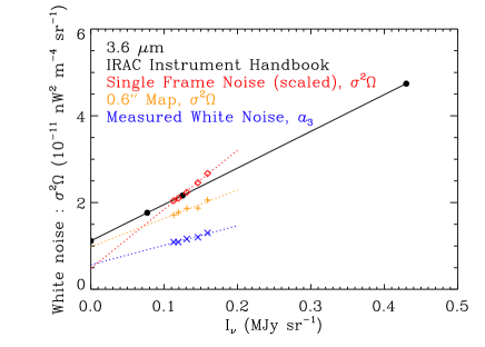
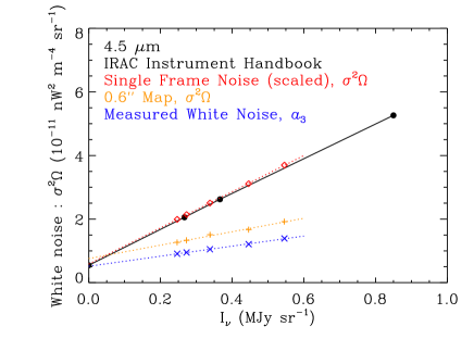
Figure 9:

the ultimate origin of the white noise component is not very important for current CIB studies, which normally subtract any “instrumental” or $A-B$ noise term that is constructed to be independent of fixed sources on the sky.

The large-scale component in the source-subtracted CIB power spectrum is the term that is of greatest cosmological interest. Prior studies agree that there is power here in excess of that expected from faint unresolved galaxies extrapolated from known galaxy populations (Kashlinsky et al., 2005; Sullivan et al., 2007; Helgason et al., 2012; Cooray et al., 2012). The lack of significant correlation between the large-scale power and the zodiacal light intensity (Figure 8) suggests that the zodiacal light is not influencing the large scale power. Additionally, we note that while the zodiacal light intensity is greater at 4.5 $\mu$m than at 3.6 $\mu$m, the data exhibit weaker large scale power at the 4.5 $\mu$m than at 3.6 $\mu$m. This also indicates that the zodiacal light is not the main source of the large scale power.

6 Summary

We have performed an experiment specifically designed to measure the impact of the zodiacal light on the estimate of the spatial fluctuations of the CIB. To provide the greatest possible sensitivity to zodiacal light effect, our test monitored a fixed patch in the COSMOS field at low ecliptic as the mean zodiacal light intensity varied over the full accessible range of brightness (or solar elongation). The CIB spatial power spectrum was calculated at 5 epochs over this 5-week interval. The power spectra are characterized as the sum of (a) a white noise component, (b) a sky shot noise component, and (c) a power component dominating on large angular scales.

We find that approximately half of the white noise component is correlated with the mean intensity of the zodiacal light. Photon shot noise of the zodiacal light is expected to be the main contribution to this correlated component. inaccuracies of the zodiacal light model in predicting the intensity in this direction as seen from Spitzer’s location within the interplanetary dust cloud.

The sky shot noise in the angular power spectra of the background is not reliably distinguished in the relatively shallow observations of this experiment. The power law component does not show significant correlation with the mean zodiacal light intensity at 3.6 or 4.5 $\mu$m. This confirms that observed spatial fluctuations at large scales ($\gtrsim 100^{\prime\prime}$) are not being influenced by zodiacal light. Prior observations had been less conclusive because they were usually limited to high ecliptic latitudes, where the zodiacal light is faintest, and to epochs $\sim 6$ or 12 months apart, where there should be minimal modulation of the zodiacal light intensity.

Appendix A Temporal Variability of the IRAC Data

Figure 4 showed that the temporally variable offset, $F^{q}$, derived by the self-calibration is accounting for variations apart from the simple trends expected of the zodiacal light. In this appendix, we demonstrate additional real trends that are being found and subtracted by the $F^{q}$ term in the self-calibration.

A.1 Zodiacal Light

The main trend expected in $F^{q}$ is the temporal variation of the zodiacal light as the solar elongation of the target field steadily increases. We model this trend as a constant times the model zodiacal light brightness (as specified by the ZODY_EST keywords in the BCD headers).

A.2 First-Frame Effect

Apart from the zodiacal light the strongest trend in $F^{q}$ is due to the “first frame effect” in the IRAC detectors. This effect appears as a variation in the background level as a function of the time since the previous exposure. It appears most strongly at the first frame in an AOR, when there has been a long slew from the previous target. The BCD pipeline attempts to correct for the first frame effect, but is not entirely successful. Here we model the first frame effect as a third-order polynomial function of the delay since the preceding frame (as specified by the FRAMEDLY keywords in the BCD headers).

A.3 Spatial Gradient

The zodiacal light has an intrinsic spatial gradient, being brighter at smaller solar elongations. During the course of dithering and moving between each of the $2\times 2$ fields of view at each epoch, locations at slightly higher and lower elongations are sampled. The corresponding variations in brightness are thus mapped as temporal variations in $F^{q}$. Additionally, the self-calibration is degenerate with respect to linear gradients across the field, which would have the same effect as the intrinsic zodiacal light gradient. We model spatial gradients in $F^{q}$ as a constant plus linear function of the $x$ and $y$ coordinates. The choice of the coordinate system is irrelevant, as the coefficients will simply adjust appropriately for any chosen system.

A.4 Exponential Decay

The final systematic effect evident in $F^{q}$ is an apparent decaying response (with a negative amplitude) across each AOR. This trend can be fit by a simple exponential decay as a function of frame number in each AOR. However, there are both fast and slow decay terms with $e$-folding constants of 9 and 70 frames. We model this decay as a linear combination of these two exponential decays. This effect was also noted by Krick et al. (2011), but it appears more cleanly here.

The net model for the temporal variation in $F^{q}$ is thus given by:

$$F^{q}_{\rm model} = A\ ZODY\_EST+$$

$$B_{1}\ FRAMEDLY+B_{2}\ FRAMEDLY^{2}+B_{3}\ FRAMEDLY^{3}+$$

$$C+D_{x}\ x+D_{y}\ y+$$

$$E_{9}\ e^{-frame/9.}+E_{70}\ e^{-frame/70.}$$

Figure 10 shows the residual $F^{q}$ after successive subtraction of each of the components of $F^{q}_{\it model}$ (with arbitrary offsets for clarity).

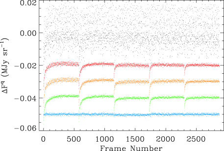
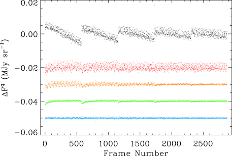
Figure 10: The successive removal of identifiable components of $F^{q}$. For 3.6 $\mu$m (left) the black dots show the full $F^{q}$ (as in Figure 4). Each segment of 576 frames corresponds to one AOR. The colored dots show the residual $F^{q}$ after successive subtraction decreasingly smaller components: a first-frame effect (red), the zodiacal light variation (orange), an arbitrary linear gradient (green), and, an exponential recovery term (blue). At 4.9 $\mu$m (right), the relative strength of the components differs and sequence shown is after successive subtractions of: the zodiacal light variation (red), a first-frame effect (orange), an arbitrary linear gradient (green), and an exponential recovery term (blue).

At 3.6 $\mu$m the first-frame effect is responsible for most of the variance in $F^{q}$, as seen by comparing the derived $F^{q}$ (black dots) with the derived $F^{q}$ minus the fitted first frame effect (red dots). At 4.5 $\mu$m, the zodiacal light trend is clearly dominant. Therefore at 4.5 $\mu$m the red dots represent the derived $F^{q}$ minus the fitted zodiacal light trend.

The comparison of the red and orange dots in both panel shows the subsequent subtraction of the zodiacal light trend (3.6 $\mu$m) and the first frame effect (4.5 $\mu$m). The zodiacal light trend has little effect at 3.6 $\mu$m. The influence of the first frame effect is now clear at 4.5 $\mu$m, though far smaller in amplitude than at 3.6 $\mu$m.

Comparison between the orange and green dots shows the subsequent subtraction of the spatial gradient terms at both wavelengths. The AORs were designed such that the spatial gradients map into oscillations with a period of 24 frames. This makes them distinguishable from the slower monotonic change in the zodiacal light intensity which occurs as a function of time. The amplitudes of the gradient terms are visibly larger in the earliest AOR and decrease across AORs as does the zodiacal light intensity.

The green dots clearly show the exponential decay behavior. At 3.6 $\mu$m, the slow 70-frame decay is evident in the first AORs, but there is a gradual transition to the faster 9-frame decay in the later AORs. At 4.5 $\mu$m, the amplitude of the decay is much smaller, and the slow 70-frame decay is dominant for all AORs.

After removal of the exponential decays, the blue dots show a fairly random distribution, with a standard deviation that is $>10$ times smaller than present in the original $F^{q}$. These residual dispersions of $\sigma=4.7\times 10^{-4}$ and $2.5\times 10^{-4}$ MJy sr^-1 represent an upper limit on the accuracy of the $F^{q}$ term of the self-calibration. The residual variation may still be accounting for real effects in the data, but the specific nature of such effects has not been identified here.

Appendix B Model Depth

A critical aspect of this analysis is the use of a source model to remove the effects of (a) the emission of extended sources and PSF wings that project beyond the masked areas, and (b) faint sources which cannot be masked without adversely decreasing the fraction of area available for analysis. Figure 11 shows power spectra of the masked images as the depth of the source model (i.e. the number of components subtracted) is linearly increased. Our choice is to use the model depth at which the skewness of the intensities of the unmasked pixel is zero. This assumes that a positive skewness signifies the presence of residual sources in the image, and that a negative skewness indicates that the model has begun subtracting the positive side of the noise distribution rather than actual sources. The zero-skewness models are evaluated independently for each epoch, and are indicated by red lines (with error bars) in Figure 11. The power spectra of the $A-B$ images are indicated by the blue lines. This figure is analogous to Figures 8 – 13 of Arendt et al. (2010).

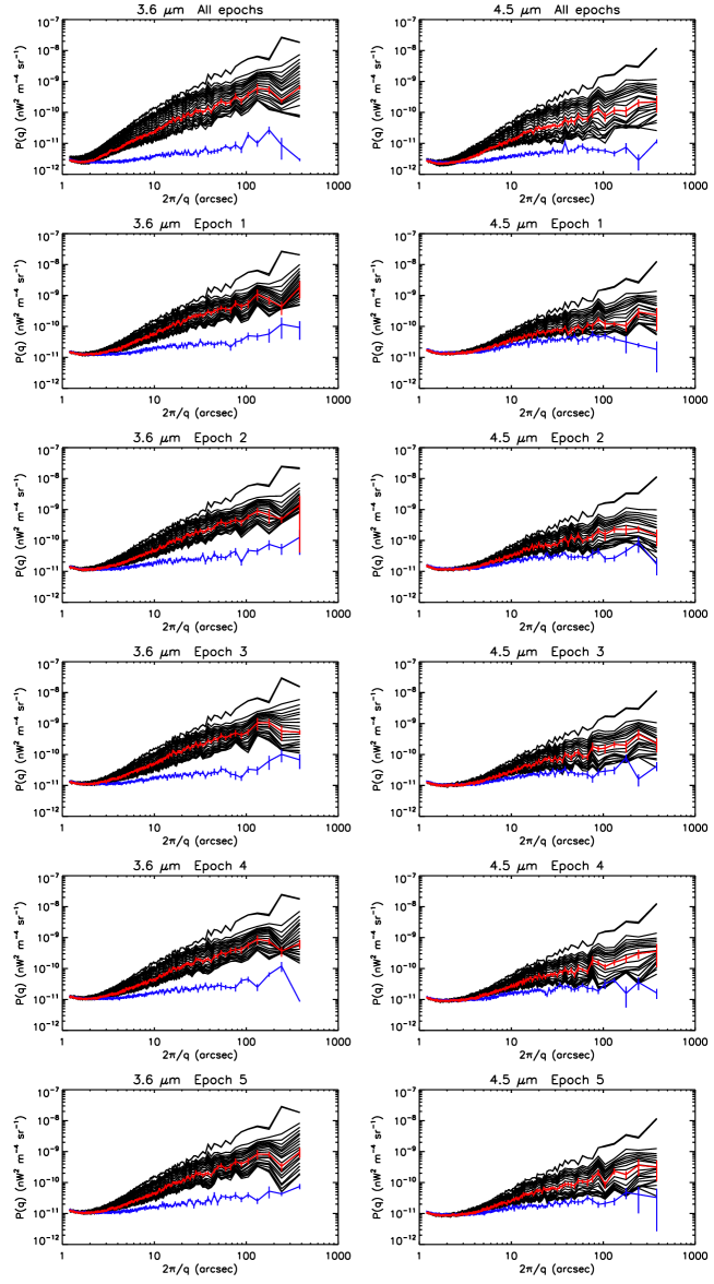
Figure 11: Power spectra shown at various model depths for the combined and separate epochs, at 3.6 $\mu$m (left) and 4.5 $\mu$m (right). The black lines show that the large scale power does drop as source model is pushed deeper. The red lines show the power spectra at “optimal” model depth when the skewness of the background (excluding outliers) is zero. The blue lines show the $A-B$ power spectra.

Appendix C Comparison to Prior Results

Figure 12 compares the power spectra measured here with those measured previously in Arendt et al. (2010). The previous power spectra are indicated by the black error bars. The power spectra measured here for epochs 1 – 5 are rainbow colored from red to blue. Magenta symbols indicate all epochs combined. The smallest scale power (dominated by white noise) decreases appropriately when all epochs are combined, whereas the large scale power is not strongly reduced by combining epochs. The large scale power is much higher than that seen in the deeper CDFS and HDFN observations, but is comparable to that of the shallower QSO1700 and EGS fields.

Figure 13 shows the same comparisons at 4.5 $\mu$m. In this case, the shot noise level of the combined epochs is similar to that observed in the deep CDFS and HDFN fields. The large scale power is also close to the levels measured in these deep fields.

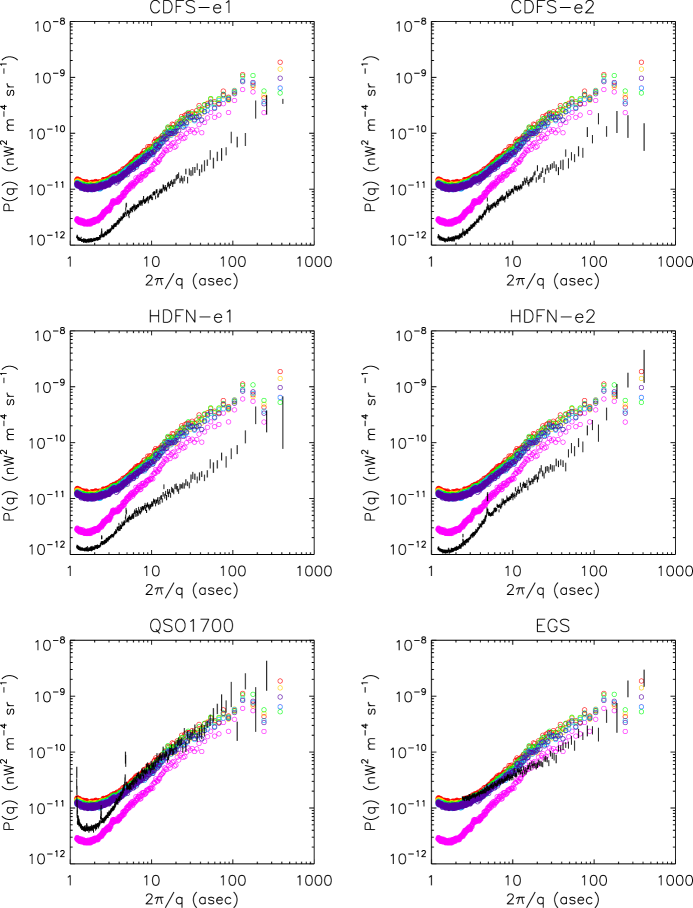
Figure 12: Comparison of the 3.6 $\mu$m power spectra measured here (red, orange, green, blue, violet, and magenta = Epochs 1, 2, 3, 4, 5, and all epochs combined), with the power spectra measured in 6 fields from Arendt et al. (2010) as indicated by the black error bars.

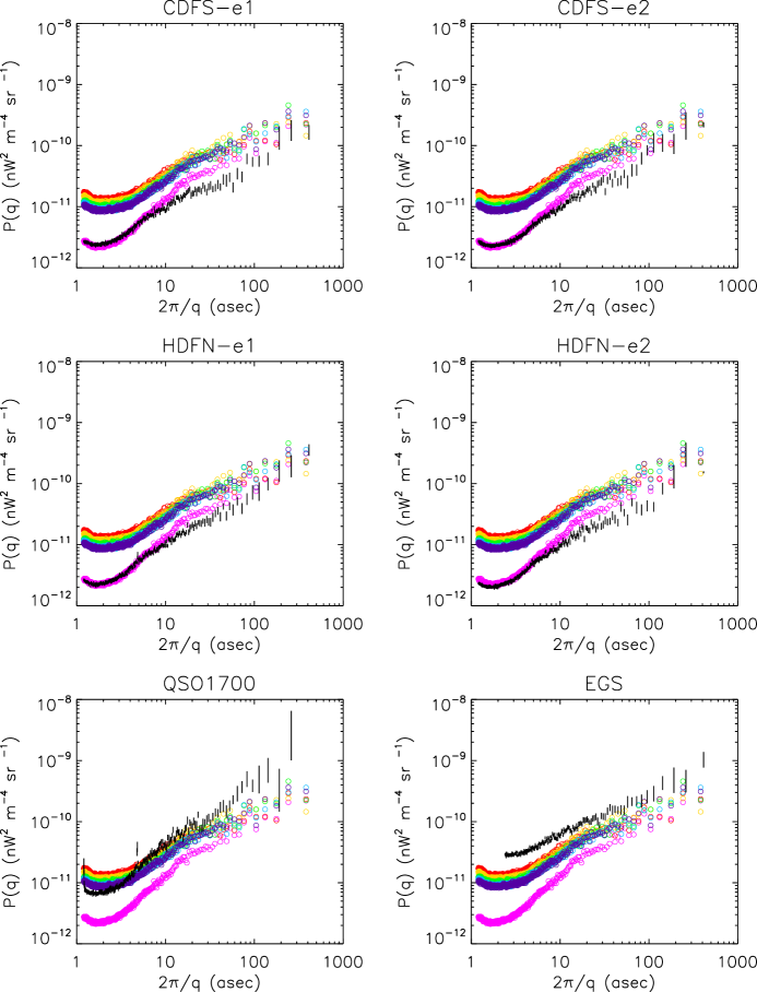
Figure 13: As Figure 12, but for 4.5 $\mu$m power spectra.

References

- Abraham et al. (1997) Abraham, P., Leinert, C., & Lemke, D. 1997, A&A, 328, 702
- Arendt et al. (2010) Arendt, R. G., Kashlinsky, A., Moseley, S. H., & Mather, J. 2010, ApJS, 186, 10
- Arendt et al. (1998) Arendt, R. G., Odegard, N., Weiland, J. L., et al. 1998, ApJ, 508, 74
- Ashby et al. (2013) Ashby, M. L. N., Willner, S. P., Fazio, G. G., et al. 2013, ApJ, 769, 80
- Ashby et al. (2015) —. 2015, ApJS, 218, 33
- Cooray et al. (2007) Cooray, A., Sullivan, I., Chary, R.-R., et al. 2007, ApJ, 659, L91
- Cooray et al. (2012) Cooray, A., Smidt, J., de Bernardis, F., et al. 2012, Nature, 490, 514
- Donnerstein (2015) Donnerstein, R. L. 2015, MNRAS, 449, 1291
- Fazio et al. (2004) Fazio, G. G., Hora, J. L., Allen, L. E., et al. 2004, ApJS, 154, 10
- Fixsen et al. (2000) Fixsen, D. J., Moseley, S. H., & Arendt, R. G. 2000, ApJS, 128, 651
- Gehrz et al. (2007) Gehrz, R. D., Roellig, T. L., Werner, M. W., et al. 2007, Review of Scientific Instruments, 78, 011302
- Hauser et al. (1998) Hauser, M. G., Arendt, R. G., Kelsall, T., et al. 1998, ApJ, 508, 25
- Helgason et al. (2012) Helgason, K., Ricotti, M., & Kashlinsky, A. 2012, ApJ, 752, 113
- Kashlinsky et al. (2012) Kashlinsky, A., Arendt, R. G., Ashby, M. L. N., et al. 2012, ApJ, 753, 63
- Kashlinsky et al. (2005) Kashlinsky, A., Arendt, R. G., Mather, J., & Moseley, S. H. 2005, Nature, 438, 45
- Kashlinsky et al. (2007) —. 2007, ApJ, 654, L5
- Kashlinsky et al. (1996a) Kashlinsky, A., Mather, J. C., & Odenwald, S. 1996a, ApJ, 473, L9
- Kashlinsky et al. (1996b) Kashlinsky, A., Mather, J. C., Odenwald, S., & Hauser, M. G. 1996b, ApJ, 470, 681
- Kashlinsky & Odenwald (2000) Kashlinsky, A., & Odenwald, S. 2000, ApJ, 528, 74
- Kashlinsky et al. (2002) Kashlinsky, A., Odenwald, S., Mather, J., Skrutskie, M. F., & Cutri, R. M. 2002, ApJ, 579, L53
- Kelsall et al. (1998) Kelsall, T., Weiland, J. L., Franz, B. A., et al. 1998, ApJ, 508, 44
- Krick et al. (2011) Krick, J. E., Bridge, C., Desai, V., et al. 2011, ApJ, 735, 76
- Krick et al. (2012) Krick, J. E., Glaccum, W. J., Carey, S. J., et al. 2012, ApJ, 754, 53
- Landsman (1993) Landsman, W. B. 1993, in Astronomical Society of the Pacific Conference Series, Vol. 52, Astronomical Data Analysis Software and Systems II, ed. R. J. Hanisch, R. J. V. Brissenden, & J. Barnes, 246
- Matsumoto et al. (2015) Matsumoto, T., Kim, M. G., Pyo, J., & Tsumura, K. 2015, ApJ, 807, 57
- Matsumoto et al. (2005) Matsumoto, T., Matsuura, S., Murakami, H., et al. 2005, ApJ, 626, 31
- Matsumoto et al. (2011) Matsumoto, T., Seo, H. J., Jeong, W.-S., et al. 2011, ApJ, 742, 124
- Matsuura et al. (2011) Matsuura, M., Dwek, E., Meixner, M., et al. 2011, Science, 333, 1258
- Mitchell-Wynne et al. (2015) Mitchell-Wynne, K., Cooray, A., Gong, Y., et al. 2015, Nature Communications, 6, 7945
- Odenwald et al. (2003) Odenwald, S., Kashlinsky, A., Mather, J. C., Skrutskie, M. F., & Cutri, R. M. 2003, ApJ, 583, 535
- Pyo et al. (2012) Pyo, J., Matsumoto, T., Jeong, W.-S., & Matsuura, S. 2012, ApJ, 760, 102
- Scoville et al. (2007) Scoville, N., Aussel, H., Brusa, M., et al. 2007, ApJS, 172, 1
- Seo et al. (2015) Seo, H. J., Lee, H. M., Matsumoto, T., et al. 2015, ApJ, 807, 140
- Sullivan et al. (2007) Sullivan, I., Cooray, A., Chary, R.-R., et al. 2007, ApJ, 657, 37
- Thompson et al. (2007a) Thompson, R. I., Eisenstein, D., Fan, X., Rieke, M., & Kennicutt, R. C. 2007a, ApJ, 657, 669
- Thompson et al. (2007b) —. 2007b, ApJ, 666, 658
- Werner et al. (2004) Werner, M. W., Roellig, T. L., Low, F. J., et al. 2004, ApJS, 154, 1
- Zemcov et al. (2014) Zemcov, M., Smidt, J., Arai, T., et al. 2014, Science, 346, 732