Geometric entanglement and quantum phase transitions
in two-dimensional quantum lattice models

Abstract

Geometric entanglement (GE), as a measure of multipartite entanglement, has been investigated as a universal tool to detect phase transitions in quantum many-body lattice models. In this paper we outline a systematic method to compute GE for two-dimensional (2D) quantum many-body lattice models based on the translational invariant structure of infinite projected entangled pair state (iPEPS) representations. By employing this method, the $q$-state quantum Potts model on the square lattice with $q\in\{2,3,4,5\}$ is investigated as a prototypical example. Further, we have explored three 2D Heisenberg models: the antiferromagnetic spin-1/2 XXX and anisotropic XYX models in an external magnetic field, and the antiferromagnetic spin-1 XXZ model. We find that continuous GE does not guarantee a continuous phase transition across a phase transition point. We observe and thus classify three different types of continuous GE across a phase transition point: (i) GE is continuous with maximum value at the transition point and the phase transition is continuous, (ii) GE is continuous with maximum value at the transition point but the phase transition is discontinuous, and (iii) GE is continuous with non-maximum value at the transition point and the phase transition is continuous. For the models under consideration we find that the second and the third types are related to a point of dual symmetry and a fully polarized phase, respectively.

I Introduction

Of the various measures of entanglement in quantum many-body systems review , geometric entanglement is a measure of the multipartite entanglement contained in a pure state. More precisely stated, the geometric entanglement (GE) quantifies the distance between a given quantum state wavefunction and the closest separable (unentangled) state review ; hba ; tcw . GE has been shown to serve as an alternative marker to locate critical points for quantum many-body lattice systems undergoing quantum phase transitions. This was demonstrated explicitly for a number of one-dimensional (1D) quantum systems wei ; ow for which the GE diverges near the critical point with an amplitude proportional to the central charge of the underlying conformal field theory at criticality central ; scopy . Moreover, for 1D quantum systems at criticality, the leading finite-size correction to the GE per lattice site is universal qqs ; jean ; hu , and related to the Affleck-Ludwig boundary entropy AL . For the Lipkin-Meshkov-Glick model, a system of mutually interacting spins embedded in a magnetic field for which analytic results can be derived, the global GE of the ground state and the single-copy entanglement behave as the entanglement entropy close to and at criticality LMG .

GE thus serves as a useful tool to investigate quantum criticality in quantum many-body lattice systems. Apart from some exceptions hl ; gehlw ; thesis ; roman ; z3pott , almost all work to date exploiting GE to study phase transitions has been restricted to quantum systems in 1D. This is mainly due to the difficulty to compute GE, because it involves a formidable optimization over all possible separable states. Indeed, the calculation of various entanglement measures has been shown recently to be NP-complete Ionnou ; Huang . This is further compounded by the inherent computational difficulties posed by two-dimensional (2D) quantum systems. Nevertheless, significant progress has been made to develop efficient numerical algorithms to simulate 2D quantum many-body lattice systems in the context of tensor network representations verstraete ; vidal ; gv2d ; jwx ; bvt ; rosgv ; pwe ; sz ; hco ; wks ; orusreview ; tn_latest . The algorithms have been successfully exploited to compute, for example, the ground-state fidelity per lattice site zhou ; zov ; jhz ; whl ; lsh , which has been established as a universal marker to detect quantum phase transitions in many-body lattice systems. Indeed, the ground state fidelity per lattice site is closely related to the GE. Therefore, it is natural to expect that there should be an efficient way to compute the GE in the context of tensor network algorithms. This has been achieved for quantum many-body lattice systems with periodic boundary conditions in one spatial dimension in the context of the matrix product state representation hu .

Quantum phase transitions in 2D quantum lattice models can be investigated using a number of different physical quantities, including local order parameters, fidelity per lattice site, single-copy entropy and multi-partite entropy measurement, and GE per lattice site. As is well known, local order parameters are defined relating to the spontaneous symmetry breaking of some symmetry group, which results in degeneracy of ground states. Different degenerate ground states can be distinguished from different values of the local order parameters, and continuous and discontinuous phase transitions can be identified from the continuous and discontinuous behavior of the local order parameters. Although demonstrated to be capable of detecting phase transitions, it is not entirely clear if GE can distinguish different degenerate ground states and identify both continuous and discontinuous quantum phase transitions.

To address this issue, we improve a systematic method gehlw to efficiently compute the GE per lattice site for 2D quantum many-body lattice systems in the context of tensor network algorithms based on an infinite projected entangled pair state (iPEPS) representation. This method is used to evaluate the GE per lattice site for a number of distinct models defined on the infinite square lattice. These models are (i) the quantum Ising model in a transverse field, (ii) the $q$-state quantum Potts model with $q=3,4$ and $5$, (iii) the spin-$\frac{1}{2}$ antiferromagnetic XXX model in an external magnetic field, (iv) the spin-$\frac{1}{2}$ antiferromagnetic XYX model in an external magnetic field, and (v) the spin-$1$ XXZ model. By comparing the behavior of the local order parameters and the GE per site for the different models, it is seen that GE can detect both continuous and discontinuous quantum phase transitions. However, we observe that the continuity of the GE per site does not necessarily match with the continuity of local order parameters.

This paper is arranged as follows. The definition of GE is given in Section II. Results using the GE per lattice site as a marker of quantum phase transitions in the various 2D quantum models on the infinite square lattice are given in Section III using the procedure outlined in Appendices A and B based on the iPEPS representation. Discussion of the results and concluding remarks are given in Section IV.

II The geometric entanglement per lattice site

For a pure quantum state $|\psi\rangle$ with $N$ parties, the GE, as a global measure of the multipartite entanglement, quantifies the deviation from the closest separable state $|\phi\rangle$. For a spin system each party could be a single spin but could also be a block of contiguous spins. The GE $E(|\psi\rangle)$ for an $N$-partite quantum state $|\psi\rangle$ is expressed as review ; hba ; tcw

$$E(|\psi\rangle)=-\log_{2}{\Lambda_{{\rm max}}^{2}},$$ (1)

where $\Lambda_{\rm max}$ is the maximum fidelity between $|\psi\rangle$ and all possible separable (unentangled) and normalized states $|\phi\rangle$, with

$$\Lambda_{{\rm max}}={\rm\max_{|\phi\rangle}}\;|\langle\psi|\phi\rangle|.$$ (2)

The GE per party ${\mathcal{E}}_{N}(|\psi\rangle)$ is then defined as

$${\mathcal{E}}_{N}(|\psi\rangle)=N^{-1}E(|\psi\rangle).$$ (3)

It corresponds to the maximum fidelity per party $\lambda^{{\rm max}}_{N}$, where

$$\lambda^{{\rm max}}_{N}=\sqrt[N]{{\Lambda_{{\rm max}}}},$$ (4)

or equivalently,

$${\mathcal{E}}_{N}(|\psi\rangle)=-\log_{2}{{(\lambda^{{\rm max}}_{N})}^{2}}.$$ (5)

The relation (1) is analogous to the relation between the free energy and the partition function. Note that for unentangled states the GE is zero.

For our purpose, we shall consider a quantum many-body system on an infinite-size square lattice, which undergoes a quantum phase transition at a critical point in the thermodynamic limit. In this situation, each lattice site constitutes a party, thus the GE per party is the GE per lattice site, which is well defined in the thermodynamic limit ($N\rightarrow\infty$), since the contribution to the fidelity from each party (site) is multiplicative. In the infinite size limit we thus denote

$${\mathcal{E}}=\lim_{N\to\infty}{\mathcal{E}}_{N}$$ (6)

as the GE per site.

III geometric entanglement in infinite square lattice systems

In this section we provide an analysis from the perspective of GE of different 2D quantum spin systems undergoing different types of quantum phase transitions. The GE per site has previously been applied to ground states of a number of 1D spin chains wei ; ow ; central ; scopy ; qqs ; jean ; hu ; hl and some 2D models hl ; gehlw ; thesis ; roman ; z3pott across primarily continuous phase transitions. Our analysis here extends these previous studies to a wider range of 2D quantum models and with more exotic situations. Previously, the GE of ground states for the quantum Ising model in a transverse field and the XYX model on the square lattice have been investigated with TRG hl and iPEPS gehlw approaches, both of which show a continuous behavior in the GE corresponding to a continuous phase transition. Our results are based on the application and improvement of an iPEPS algorithm for the calculation of the GE of 2D quantum systems gehlw , as detailed in Appendices A and B. Preliminary results along this direction were also reported in Ref. thesis . The size of the truncation dimension $D$ controls the underlying accuracy of the iPEPS algorithm. For the purposes of this study, which focusses on the general behavior of the GE in the vicinity of quantum critical points, we consider sufficiently large values of $D$, compared to Refs. gehlw ; thesis , to be confident of the observed behavior. Refinements in the implementation of the basic iPEPS algorithm have been discussed recently tn_latest .

III.1 2D quantum Ising model in a transverse field

We consider the hamiltonian

$$H=-\sum_{(\vec{r},\vec{r}^{\prime})}S^{[\vec{r}]}_{x}S^{[\vec{r}^{\prime}]}_{x}-\lambda\sum_{\vec{r}}S^{[\vec{r}]}_{z},$$ (7)

where here and in later subsections $S^{[\vec{r}]}_{\alpha}(\alpha=x,y,z)$ are spin-$\frac{1}{2}$ Pauli operators acting at site $\vec{r}$, with $(\vec{r},\vec{r}^{\prime})$ running over all possible nearest-neighbor pairs on the square lattice. The parameter $\lambda$ measures the strength of the transverse magnetic field, with a phase transition from a ferromagnetic phase with two degenerate ground states to a paramagnetic phase with a single ground state occurring at the critical value $\lambda_{c}$. This model has been widely studied via a number of different techniques. Of particular relevance here are the previous calculation of the GE using the tensor product state and tensor renormalization group approach hl and iPEPS gehlw ; thesis .

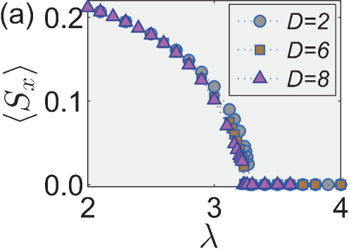
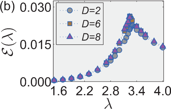
Figure 1: (color online) Numerical values for (a) the local order parameter $\langle S_{x}\rangle$ and (b) the GE per site ${\mathcal{E}}_{\infty}(\lambda)$ for the 2D quantum Ising model as a function of the transverse field strength $\lambda$ for the indicated values of the iPEPS truncation dimension $D$.

For different values of the truncation dimension $D$, when $\lambda<\lambda_{c}(D)$, spontaneous symmetry breaking occurs with $S_{x}$ the unitary element of the broken $Z_{2}$ symmetry group. Thus two degenerate ground states are detected and distinguished by the sign of the local order parameter $\langle S_{x}\rangle$, with the amplitude associated with each of the two degenerate ground states having the same value. The order parameter $\langle S_{x}\rangle$ is shown in Fig. 1(a). Phase transition points are identified at the values shown in Table I. Near these points the amplitude of $\langle S_{x}\rangle$ is observed to continuously approach zero, indicative of a continuous phase transition.

On the other hand, the estimates for the GE per lattice site for the ground states are shown in Fig. 1(b). For each value of $D$ the GE curve has a maximal value at $\lambda_{c}(D)$, which indicate the phase transition points. These values, shown in Table I, agree with the values detected with the local order parameter. Our results are consistent with the previous studies hl ; gehlw ; thesis . The GE is seen to be continuous near the maximal points. The cusp-like behavior at the critical point is a characteristic feature of the GE at a continuous phase transition. The two degenerate ground states for $\lambda<\lambda_{c}$ can also be distinguished via the initial random states.

Table 1: Estimates of critical points $\lambda_{c}$ for the $q$-state quantum Potts model on the square lattice. The values for $\lambda_{c}(D)$ follow from the behavior of the local order parameter and the GE per site, where $D$ is the iPEPS truncation dimension.

		$D$	$\lambda_{c}(D)$
	$q=2$	2	3.28
		6	3.235
		8	3.23
	$q=3$	3	2.620
		6	2.616
		9	2.616
	$q=4$	4	2.430
		8	2.428
		10	2.426
	$q=5$	5	2.330
		8	2.326
		10	2.326

III.2 2D $q$-state quantum Potts model

The quantum Ising model discussed above is the special $q=2$ case of the more general $q$-state quantum Potts model defined on the square lattice. For a regular lattice, classical mean-field solutions Wu and extensive computations (see, e.g., Refs. Wu ; dyw and references therein) have suggested that the 3D classical $q$-state Potts model, and thus the 2D $q$-state quantum version, undergo a continuous phase transition for $q\leq 2$ and a discontinuous phase transition for $q>2$. We now turn to this 2D $q$-state quantum model and examine the GE per site and local order parameters in the vicinity of the phase transition points for the values $q=3,4$ and $5$.

On the square lattice the hamiltonian can be written in the form

$$H=-\sum_{(\vec{r},\vec{r}^{\prime})}\left(\sum_{p=1}^{q-1}M^{[\vec{r}]}_{x,p}M^{[\vec{r}^{\prime}]}_{x,q-p}\right)-\lambda\sum_{\vec{r}}M^{[\vec{r}]}_{z},$$ (8)

where $M^{[\vec{r}]}_{x,p}$ and $M^{[\vec{r}]}_{z,p}$, with $p=1,\ldots,q-1$, are spin matrices of size $q\times q$ acting at site $\vec{r}$. The parameter $\lambda$ is the analogue of the transverse magnetic field in the Ising case. In this formulation the spin matrices acting at each site are given by qPotts

$$M_{x,1}=\left(\begin{array}[]{cc}0&I_{q-1}\\ 1&0\end{array}\right),\quad M_{z}=\left(\begin{array}[]{cc}q-1&0\\ 0&-I_{q-1}\end{array}\right),$$

where $I_{q-1}$ is the $(q-1)\times(q-1)$ identity matrix with $M_{x,p}=\left(M_{x,1}\right)^{p}$ and $\left(M_{x,1}\right)^{q}=I_{q}$.

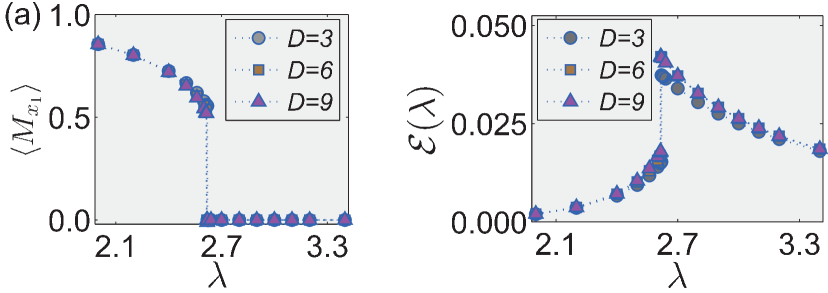
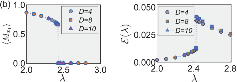
Figure 2: (color online) Numerical values for the local order parameter $\langle M_{x_{1}}\rangle$ and the GE per site ${\mathcal{E}}(\lambda)$ for the 2D quantum $q$-state Potts model for (a) $q=3$, (b) $q=4$ and (c) $q=5$ as a function of the transverse field strength $\lambda$ for the indicated values of the iPEPS truncation dimension $D$. For each case the curves for both the local order parameter and the GE show a discontinuous behavior, indicative of a discontinuous phase transition.

Denoting the phase transition point by $\lambda_{c}$ we expect to detect $q$-degenerate ground states for $\lambda<\lambda_{c}$, corresponding to a $Z_{q}$ broken symmetry phase. The local order parameter $\langle M_{x,1}\rangle$ can distinguish the different degenerate ground states, but with the same amplitude for each of the $q$ ground states. As for the $q=2$ case, the phase transition point $\lambda_{c}(D)$ is estimated with increasing truncation dimension $D$. Fig. 2(a) shows the amplitude of the local order parameter $\langle M_{x,1}\rangle$ for the 3-state Potts model. This plot shows a jump in the curve which indicates a possible discontinuous phase transition point. The successive estimates for $\lambda_{c}$ are given in Table I ZN . This same type of discontinuous behavior is seen for the local order parameter $\langle M_{x,1}\rangle$ in Fig. 2(b) for $q=4$ and Fig. 2(c) for $q=5$. The successive estimates for $\lambda_{c}$ are given in Table I.

The GE of the ground states is also shown in Fig. 2. For each of the values of $q$, a maximal value is detected for the GE curve, where a jump also occurs. The estimates for the transition points $\lambda_{c}$ are well matched with those obtained via the local order parameters and also via the observed multi-bifurcation points in the magnetization dyw . It is clear that the measure of GE can distinguish between discontinuous and continuous phase transitions in the 2D quantum $q$-state Potts model. To further test the utility of this approach we turn now to the investigation of GE in other 2D quantum models.

III.3 2D spin-$\frac{1}{2}$ XXX model in a magnetic field

The spin-$\frac{1}{2}$ antiferromagnetic XXX model on the square lattice has hamiltonian

$$H=\sum_{(\vec{r},\vec{r}^{\prime})}\left(S^{[\vec{r}]}_{x}S^{[\vec{r}^{\prime}]}_{x}+S^{[\vec{r}]}_{y}S^{[\vec{r}^{\prime}]}_{y}+S^{[\vec{r}]}_{z}S^{[\vec{r}^{\prime}]}_{z}\right)-h\sum_{\vec{r}}S^{[\vec{r}]}_{z},$$ (9)

where $h$ is an external magnetic field along the $z$ direction. This model has been studied via a barrage of different techniques sandvik . Whereas magnetic order is normally ruled out in 1D Heisenberg models, this is not the case for 2D Heisenberg models mermin ; sandvik . Thus in 2D the ground state can be non-magnetic, i.e., with a non-zero magnetization. In the absence of the magnetic field the ground state of the Heisenberg model has antiferromagnetic (Néel) order with a non-zero local staggered magnetization and infinitely degenerate ground states resulting from the breaking of global SU$(2)$ spin rotation symmetry. For $h\neq 0$, infinitely degenerate ground states are detected resulting from the spontaneous symmetry breaking of U$(1)$ symmetry in the $x$-$y$ plane. As $h\rightarrow\infty$ it is anticipated the system will be fully polarized in the $z$ direction. In fact this transition to the fully polarized state occurs at $h=4$.

In Fig. 3(a) we show the local magnetizations for sublattices A and B defined by $m_{\alpha}^{A}=\langle S_{\alpha}^{A}\rangle$ and $m_{\alpha}^{B}=\langle S_{\alpha}^{B}\rangle$ for $\alpha=x,y,z$. For $h<4$, $m_{\alpha}^{A}=-m_{\alpha}^{B}$ for $\alpha=x,y$ with $m_{z}^{A}=m_{z}^{B}$. For $h>4$, $m_{\alpha}^{A}=m_{\alpha}^{B}=0$ for $\alpha=x,y$ with $m_{z}^{A}=m_{z}^{B}=\frac{1}{2}$. The latter is indicative of the fully polarized state.

In Fig. 3(b) we show the staggered magnetization parameters $M_{xy}=\sqrt{\langle\frac{1}{2}(S_{x}^{A}-S_{x}^{B})\rangle^{2}+\langle\frac{1}{2}(S_{y}^{A}-S_{y}^{B})\rangle^{2}}$ and $M_{z}=\langle\frac{1}{2}(S_{z}^{A}+S_{z}^{B})\rangle$ as functions of the magnetic field. The local order parameter $M_{xy}$ decreases with increasing $h$, with $M_{xy}\to 0$ when $h>4$. On the other hand, $M_{z}$ increases with increasing $h$, with $M_{z}\to\frac{1}{2}$ for $h>4$, which corresponds to a continuous phase transition from a Néel phase to the fully polarized phase. As mentioned previously, for $h<4$, infinitely degenerate ground states exist corresponding to the $x$-$y$ plane U$(1)$ symmetry breaking, which is indicated from the random-like magnetization on the sublattices. As for the previous models, the numerical results indicate that the different degenerate ground states for fixed $h$ give the same value for the GE per site, as Fig. 3(c) shows. In Fig. 3(c), the GE per site clearly decreases with increasing $h$, indicating decreasing entanglement as $h\to 4$. In fact, zero GE per site indicates a factorizing field, in this case the simple polarized state. This factorizing field is discussed further below in the context of the more general $XYX$ model.

In contrast to the previous models studied here, the GE is not maximal at the phase transition point, because the phase transition point is not the critical point which would correspond to maximum entanglement. In this case zero or nonzero GE per site distinguishes between the two different phases in the model.

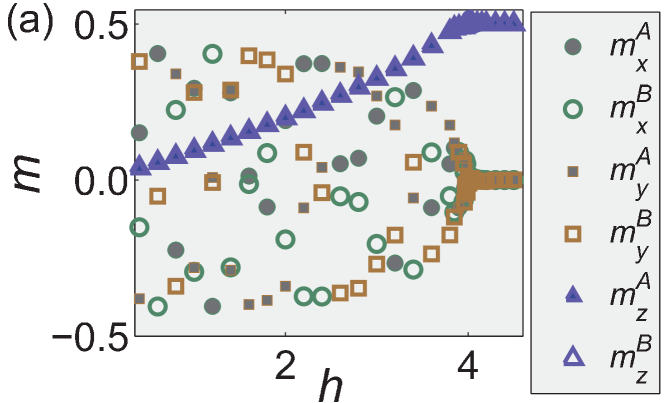
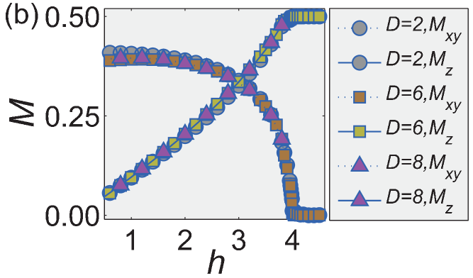
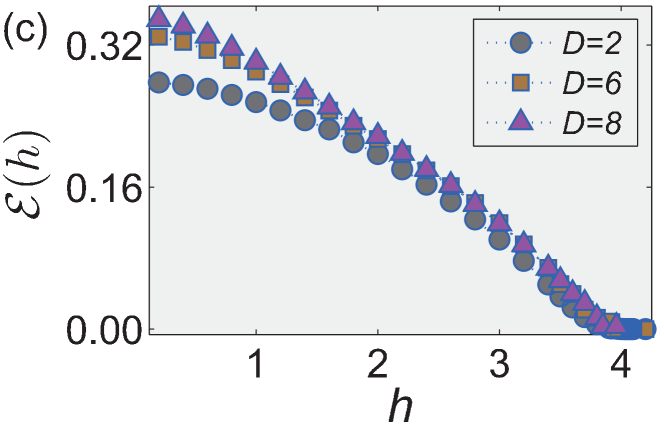
Figure 3: (color online) Plots for the 2D spin-$\frac{1}{2}$ XXX model with varying magnetic field $h$. (a) Local magnetization $m$ for sublattices A and B, obtained with iPEPS truncation dimension $D=2$. (b) Amplitude of the local order parameters $M$. (c) GE per site ${\mathcal{E}}(h)$.

III.4 2D spin-$\frac{1}{2}$ XYX model in a magnetic field

Tuning the anisotropy of the Heisenberg interactions leads to the more general spin-$\frac{1}{2}$ XYX antiferromagnetic model in a uniform magnetic field, defined on the square lattice by the hamiltonian

$$H=\sum_{(\vec{r},\vec{r}^{\prime})}\left(S^{[\vec{r}]}_{x}S^{[\vec{r}^{\prime}]}_{x}+\Delta_{y}S^{[\vec{r}]}_{y}S^{[\vec{r}^{\prime}]}_{y}+S^{[\vec{r}]}_{z}S^{[\vec{r}^{\prime}]}_{z}\right)-h\sum_{\vec{r}}S^{[\vec{r}]}_{z}.$$ (10)

Varying the anisotropic exchange interaction parameter $\Delta_{y}$ leads to different behavior, with the two cases $\Delta_{y}<1$ and $\Delta_{y}>1$ corresponding to an easy-plane and easy-axis behavior, respectively. The quantum criticality of this model is well understood tros , with an ordered phase below a critical field value $h_{c}$, above which is a partially polarized state with field-induced magnetization reaching saturation as $h\to\infty$. The ordered phase in the easy-plane (easy-axis) case arises by spontaneous symmetry breaking along the $x$ ($y$) direction, which corresponds to a finite value of the order parameter $M_{x}$ ($M_{y}$) below $h_{c}$. At the transition point $h_{c}$, long-range correlations are destroyed.

Previous studies of this model using GE gehlw ; hl focussed on the value $\Delta_{y}=0.25$ with the magnetic field as control parameter. In this easy-plane region the model is known to undergo a continuous quantum phase transition in the same universality class as the transverse Ising model tros . The GE was seen to have a cusp at the critical value $h_{c}$ gehlw ; hl as observed for the transverse Ising model (recall Fig. 1(b)). Significantly, it is known that a factorizing field exists at the value $h_{f}=2\sqrt{2(1+\Delta_{y})}$, with $h_{f}<h_{c}$, where the ground state becomes a separable product state tros . At this point it follows that the GE vanishes, i.e., ${\mathcal{E}}_{\infty}(h_{f})=0$. This was observed in the simulations using GE gehlw ; hl . Other entanglement measures were also confirmed to vanish at this point tros ; lsh .

In this study we consider the fixed parameter value $h=0.25$ and vary the coupling $\Delta_{y}$. The model is anticipated to undergo a transition at $\Delta_{y}=1$ from an antiferromagnetic phase in the $x$ direction to an antiferromagnetic phase in the $y$ direction, with local order parameter the staggered magnetization $M_{x}$ ($M_{y}$) corresponding to the phase $\Delta_{y}<1$ ($\Delta_{y}>1$).

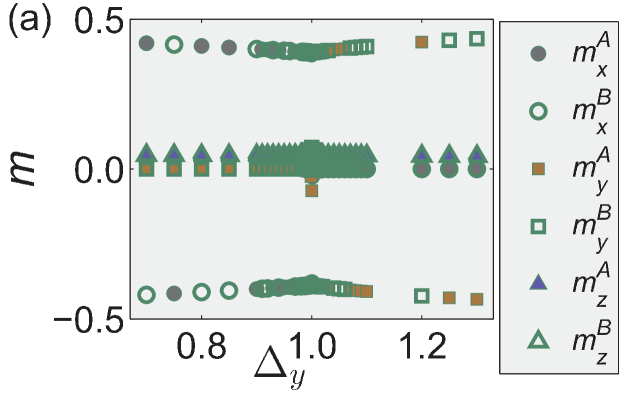
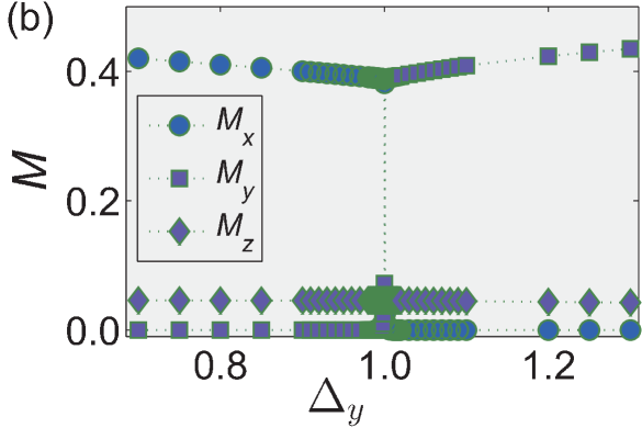
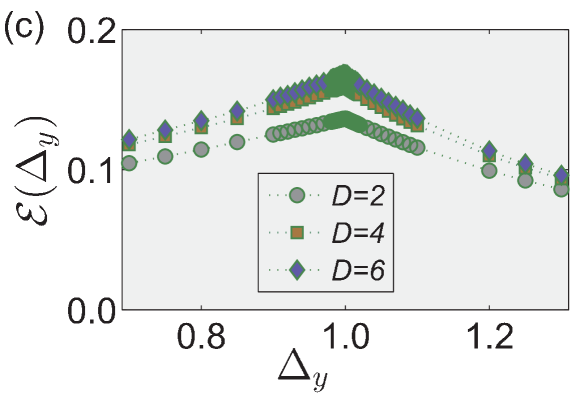
Figure 4: (color online) Plots for the spin-$\frac{1}{2}$ XYX model with fixed magnetic field $h=0.25$ and varying anisotropy parameter $\Delta_{y}$. (a) Components of the local magnetization $m$ for sublattices A and B for truncation dimension $D=6$. (b) Components of the staggered magnetizations $M$ for truncation dimension $D=6$. (c) GE per site ${\mathcal{E}}(\lambda)$ with truncation dimension $D$.

Fig. 4(a) shows the components of the local magnetization for sublattices A and B defined by $m_{\alpha}^{A}=\langle S_{\alpha}^{A}\rangle$ and $m_{\alpha}^{B}=\langle S_{\alpha}^{B}\rangle$ for $\alpha=x,y,z$. For $\Delta_{y}<1$, $m_{x}^{A}$ and $m_{x}^{B}$ have opposite values, with $m_{y}^{A}=m_{y}^{B}=0$ and $m_{z}^{A}=m_{z}^{B}$. This implies that a staggered magnetization $M_{x}=\langle\frac{1}{2}(S_{x}^{A}-S_{x}^{B})\rangle$ exists. For $\Delta_{y}>1$, $m_{y}^{A}$ and $m_{y}^{B}$ have opposite values, with $m_{x}^{A}=m_{x}^{B}=0$ and $m_{z}^{A}=m_{z}^{B}$, implying the staggered magnetization $M_{y}=\langle\frac{1}{2}(S_{y}^{A}-S_{y}^{B})\rangle$. These magnetizations are shown in Fig. 4(b) for the two different phases for truncation dimension $D=6$. There is a clear jump discontinuity at $\Delta_{y}=1$ for each of the staggered magnetizations $M_{x}$ and $M_{y}$. This behavior persists with increasing truncation dimension $D$, indicating a discontinuous phase transition at $\Delta_{y}=1$.

The GE per site is shown for the same parameter range in Fig. 4(c) with increasing truncation dimension. The characteristic cusp occurs as $\Delta_{y}$ varies across the critical point $\Delta_{y}=1$. In contrast to the local order parameter, which is discontinuous, the GE is continuous. In this case the GE thus does not detect the discontinuous behavior at the phase transition point.

III.5 2D spin-$1$ XXZ model

The spin-$1$ XXZ model is defined on the square lattice by the hamiltonian

$$H=\sum_{(\vec{r},\vec{r}^{\prime})}\left(S^{[\vec{r}]}_{x}S^{[\vec{r}^{\prime}]}_{x}+S^{[\vec{r}]}_{y}S^{[\vec{r}^{\prime}]}_{y}+\Delta S^{[\vec{r}]}_{z}S^{[\vec{r}^{\prime}]}_{z}\right),$$ (11)

where now $S^{[\vec{r}]}_{\alpha}(\alpha=x,y,z)$ are spin-$1$ operators at site $\vec{r}$, with again the summation running over all nearest neighbor pairs on the square lattice. For anisotropic exchange interaction parameter $\Delta=1$ the hamiltonian has $SU(2)$ symmetry and the ground state is infinitely degenerate. For this model there is a quantum phase transition at $\Delta=1$ spin1 . This phase transition is clearly marked in Fig. 5, which shows plots of the single-copy entanglement for the spin-$1$ XXZ model.

We also calculate the components of the local magnetization $m$ for sublattices $A$ and $B$: $m_{\alpha}^{A}=\langle S_{\alpha}^{A}\rangle$ and $m_{\alpha}^{B}=\langle S_{\alpha}^{B}\rangle$ for $\alpha=x,y,z$. These are shown in Fig. 6(a) as a function of $\Delta$. For $\Delta<1$, the values of $m_{x}$ and $m_{y}$ have opposite signs on each sublattice, with $m_{z}^{A}=m_{z}^{B}$. For $\Delta>1$, $m_{x}=m_{y}=0$ on each sublattice, with $m_{z}^{A}=-m_{z}^{B}$. This indicates a local order with staggered magnetization in the $z$ phase characterized by $M_{z}=\langle\frac{1}{2}(S_{z}^{A}-S_{z}^{B})\rangle.$ For different values of magnetic field strength $h$, the magnetization for the $x$ and $y$ directions does not change continuously for $\Delta<1$, while the staggered magnetization $M_{xy}=\sqrt{\langle\frac{1}{2}(S_{x}^{A}-S_{x}^{B})\rangle^{2}+\langle\frac{1}{2}(S_{y}^{A}-S_{y}^{B})\rangle^{2}},$ continuously changes with varying $\Delta$ (see Fig. 6(b)). This indicates the existence of local order defined with the staggered magnetization in the $x$-$y$ plane.

Hence, for $\Delta<1$, the phase is characterized by the antiferromagnetic order parameter $M_{xy}$ in the $x$-$y$ easy plane. Infinitely degenerate ground states exist corresponding to the $x$-$y$ plane $U(1)$ symmetry breaking, indicated from the random-like magnetization of sublattices as shown in Fig. 6(a). For $\Delta>1$, the phase is characterized by the antiferromagnetic order parameter $M_{z}$ along the easy axis, with doubly degenerate ground states corresponding to the spin-flip (or one-site translational invariant) $Z_{2}$ symmetry breaking. These order parameters are shown in Fig. 6(b). For each truncation dimension, a distinct jump is detected at $\Delta=1$, indicating the phase transition is possibly discontinuous. The total antiferromagnetic order parameter $M_{t}=\sqrt{\langle\frac{1}{2}(S_{x}^{A}-S_{x}^{B})\rangle^{2}+\langle\frac{1}{2}(S_{y}^{A}-S_{y}^{B})\rangle^{2}+\langle\frac{1}{2}(S_{z}^{A}-S_{z}^{B})\rangle^{2}}$ is shown in Fig. 6(c). It varies continuously.

For comparison we also consider the GE per site for this model. The GE per site is seen to take the same value for all of the degenerate ground states. As shown in Fig. 6(d), the GE is continuous with a well defined cusp at the point $\Delta=1$, while the local order parameters in Fig. 6(b) are discontinuous at $\Delta=1$. This behavior is similar to that observed in the previous subsection for the 2D spin-$\frac{1}{2}$ XYX model with fixed magnetic field $h$.

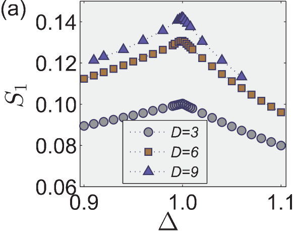
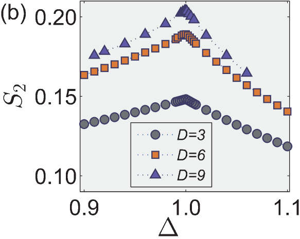
Figure 5: (color online) Single-copy entanglement (a) $S_{1}(\Delta)$ and (b) $S_{2}(\Delta)$ as a function of the anisotropy parameter $\Delta$ for the 2D spin-$1$ XXZ model with increasing iPEPS truncation dimension $D$. Here the single-copy entanglement is calculated based on the one-site and two-site reduced density matrix, obtained by using the iTEBD method.

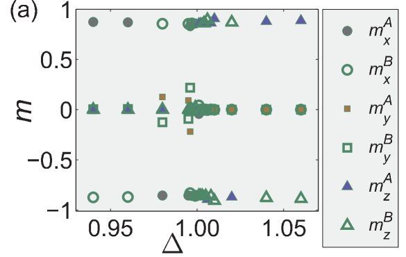
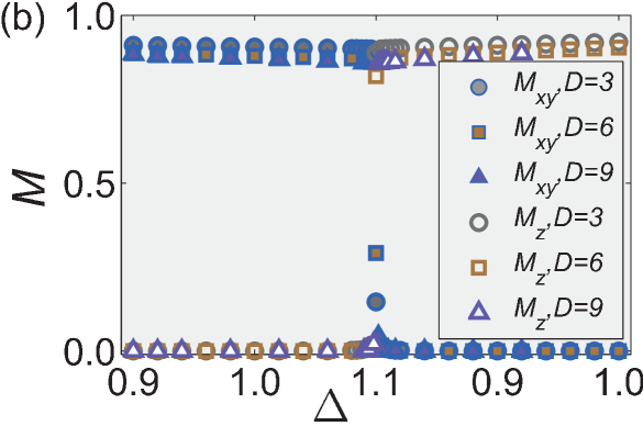
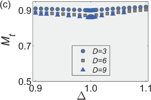
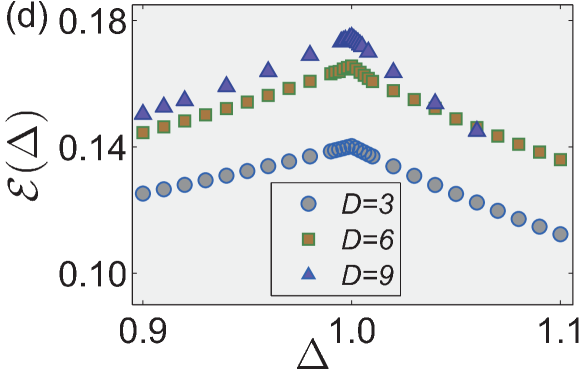
Figure 6: (color online) (a) Sublattice components of the local magnetization $m$, (b) amplitude of the local order parameters $M_{xy}$ and $M_{z}$, (c) total antiferromagnetic order parameter $M_{t}$ and (d) GE per lattice site ${\mathcal{E}}(\Delta)$ as a function of anisotropy parameter $\Delta$ for the 2D spin-$1$ XXZ model. Values of the iPEPS truncation dimension $D$ are as indicated, with $D=9$ for (a).

IV summary and discussion

We have demonstrated how to efficiently compute the GE of 2D quantum models defined on the infinite square lattice, by optimizing over all possible separable states, in the context of the tensor network algorithm based on the iPEPS representation. Our results, in line with previous studies hl ; gehlw ; thesis ; roman ; z3pott , demonstrate that GE is able to detect continuous quantum phase transitions and factorized fields for different 2D quantum systems. Continuous phase transitions are marked by a characteristic continuous cusp-like behavior of the GE per site at the critical point. This behavior is evident in Fig. 1(b) for the 2D quantum Ising model in a transverse field. Additionally we have demonstrated that the GE can detect discontinuous phase transitions in the $q$-state quantum Potts model for $q\geq 3$. For the values of $q$ considered, a maximal value is detected for the GE curve, where the discontinuous transition occurs (see Fig. 2). It is thus clear that the measure of GE can distinguish between continuous and discontinuous phase transitions in the 2D quantum $q$-state Potts model.

This overall picture is not so simple, however. It has been demonstrated recently that quantum phase transitions should be treated with caution, at least with regard to the ground state entanglement spectrum CKS2014 . In the present study, we have seen an example where the GE is continuous with non-maximum value at the transition point and the phase transition is continuous. This is the case for the spin-$\frac{1}{2}$ XXX model, for which the GE is not maximal at the phase transition point $h=4$ at which the GE vanishes (see Fig. 3(c)). We have also seen examples where the GE per site shows continuous behavior at discontinuous phase transition points. For example, in the spin-$\frac{1}{2}$ XYX model and the spin-$1$ XXZ model, the GE per site shows continuous behavior with well defined cusps at the transition point (Fig. 4(c) and Fig. 6(d)) but the corresponding local staggered magnetizations (Fig. 4(b) and Fig. 6(b)) are discontinuous. We have also considered the single-copy entanglement $S_{L}$, in which the system under consideration is divided into two parts, one with $L$ lattice sites and the other with the other lattice sites. It is known that the single-copy entanglement $S_{L}$ sets a bound for the GE scopy , i.e., ${\cal E}<S_{L}=-\log_{2}{\mu_{L}^{1}}$, with $\mu_{L}^{1}$ the largest eigenvalue of the reduced density matrix $\rho_{L}$ for an $L$-site subsystem. It is found that the single-copy entanglements $S_{1}$ and $S_{2}$ show the same continuous behavior near the phase transition points for the models considered here, as shown, e.g., in Fig. 5 for the spin-$1$ XXZ model. It appears then for such systems, for which discontinuous phase transitions occur corresponding to different types of symmetry breaking and the total magnetization is continuous, both multi-partite and bi-partite entanglement measures are continuous.

This situation can be further understood as follows. First, as already mentioned, due to the spontaneous symmetry breaking, including the spontaneous breaking of continuous symmetry, different degenerate ground states are detected in the broken symmetry phase by different values of the local order parameter. However, the GE takes the same value for all degenerate ground states. In terms of entanglement, this can be understood from the GE being a global measure of entanglement, which is the same for all degenerate ground states. From a different perspective, we can suppose the closest separable state to the ground state and the ground states share some property, i.e., we suppose the closest separable state of different degenerate ground states breaks the same symmetry of the ground states .

Also from the perspective of symmetry, it could be argued for the spin-$\frac{1}{2}$ XYX model and the spin-$1$ XXZ model that the discontinuity due to the isometry cannot be detected with the GE measure because the hamiltonian/ground state obeys a dual symmetry either side of the phase transition point. For the spin-$\frac{1}{2}$ XYX model this symmetry is in $\Delta_{y}$, with $\Delta_{y}=1$ the “self-dual” point . Given such a duality of the hamiltonian, both the ground state and its closest separable state are also each dual under this transformation, so the fidelity between the ground state and its closest separable state also obeys the same relation, leading to continuous behavior across the phase transition point. Similarly for the spin-$1$ XXZ model, the hamiltonian is symmetric at $\Delta=1$, with $\Delta\neq 1$ breaking the symmetry into easy-plane and easy-axis. In this case such a duality in the total staggered magnetization of the easy-plane and easy-axis would imply a duality of a local property of the ground state wavefunction, leading to continuity in the GE.

We have seen then three different types of continuous GE across a phase transition point:

(i) GE is continuous with maximum value at the transition point and the phase transition is continuous,

(ii) GE is continuous with maximum value at the transition point but the phase transition is discontinuous, and

(iii) GE is continuous with non-maximum value at the transition point and the phase transition is continuous.

For the models under consideration the second and third types are related to a point of dual symmetry and a fully polarized phase, respectively. Given this refinement in our understanding of GE as a marker of quantum phase transitions, and the development of powerful tensor network algorithms, we can be confident that GE can be used as an alternative route to explore quantum criticality in quantum lattice models.

Acknowledgements. MTB gratefully acknowledges support from Chongqing University and the 1000 Talents Program of China. This work is supported in part by the National Natural Science Foundation of China (Grant Numbers 11575037, 11374379 and 11174375).

Appendix  A The infinite projected entangled pair state algorithm

Our aim is to compute the GE per lattice site for a quantum many-body lattice system on an infinite-size square lattice in the context of the iPEPS algorithm gv2d . Here we follow the presentation given in Ref. gehlw .

Suppose we consider a system characterized by a translation-invariant Hamiltonian $H$ with nearest-neighbor interactions: $H=\sum_{\langle ij\rangle}h_{\langle ij\rangle}$, with $h_{\langle ij\rangle}$ being the Hamiltonian density. Assume that a quantum wavefunction $|\psi\rangle$ is translation-invariant under two-site shifts, then one only needs two five-index tensors $A^{s}_{lrud}$ and $B^{s}_{lrud}$ to express the iPEPS representation. Here, each tensor is labeled by one physical index $s$ and four bond indices $l$, $r$, $u$ and $d$, as shown in Fig. 7(i). Note that the physical index $s$ runs over $1,\ldots,\mathrm{d}$, and each bond index takes $1,\ldots,D$, with $\mathrm{d}$ being the physical dimension, and $D$ the bond dimension. Therefore, it is convenient to choose a $2\times 2$ plaquette as the unit cell (cf. Fig. 7(ii)). The ground state wavefunction is well approximated by $|\psi_{\tau}\rangle$, which is obtained by performing an imaginary time evolution gv2d from an initial state $|\psi_{0}\rangle$, with $|\psi_{\tau}\rangle=e^{-H\tau}|\psi_{0}\rangle/||e^{-H\tau}|\psi_{0}\rangle||$ gv2d , as long as $\tau$ is large enough.

A key ingredient of the iPEPS algorithm is to take advantage of the Trotter-Suzuki decomposition that allows to reduce the (imaginary) time evolution operator $e^{-H\delta\tau}$ over a time slice $\delta\tau$ into the product of a series of two-site operators, where the imaginary time interval $\tau$ is divided into $M$ slices: $\tau=M\delta\tau$. Therefore, the original global optimization problem becomes a local two-site optimization problem. With an efficient contraction scheme available to compute the effective environment for a pair of the tensors $A^{s}_{lrud}$ and $B^{s}_{lrud}$ gv2d , one is able to update the tensors $A^{s}_{lrud}$ and $B^{s}_{lrud}$. Performing this procedure until the energy per lattice site converges, the ground state wavefunction is produced in the iPEPS representation.

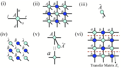
Figure 7: (color online) (i) A five-index tensor $A^{s}_{lrud}$ labeled by one physical index $s$ and four bond indices $l$, $r$, $u$ and $d$. (ii) The iPEPS representation of a wavefunction on the square lattice. Copies of the tensors $A^{s}_{lrud}$ and $B^{s}_{lrud}$ are connected through four types of bonds. (iii) A one-index tensor $\tilde{A}^{s}$ labeled by one physical index $s$. (iv) The iPEPS representation of a separable state in the square lattice. (v) A reduced four-index tensor $a_{lrud}$ from a five-index tensor $A^{s}_{lrud}$ and a one-index $\tilde{A}^{s*}$. (vi) The tensor network representation for the fidelity between a quantum wavefunction (described by $A^{s}_{lrud}$ and $B^{s}_{lrud}$) and a separable state (described by $\tilde{A}^{s}$ and $\tilde{B}^{s}$), consisting of the reduced tensors $a_{lrud}$ and $b_{lrud}$.

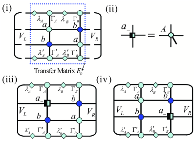
Figure 8: (color online) Key ingredients for obtaining the gradient of the fidelity between a given ground state wavefunction $|\psi\rangle$ and a separable state $|\phi\rangle$ in the iPEPS representation. (i) Zero-dimensional transfer matrix $E_{0}$ and its dominant eigenvectors $V_{L}$ and $V_{R}$. Here the infinite matrix product state representation of the dominant eigenvectors for the one-dimensional transfer matrix $E_{1}$ follows from Ref. rosgv , and $V_{L}$ and $V_{R}$ may be evaluated using the Lanczos method. The contraction of the entire tensor network is the dominant eigenvalue $\eta_{\langle\phi|\psi\rangle}$ of the zero-dimensional transfer matrix $E_{0}$ for $\langle\phi|\psi\rangle$. (ii) A half-filled square denotes $a_{-}$, the derivative of the four-index tensor $a_{lrud}$ with respect to $\tilde{A}^{s*}$, which is nothing but the five-index tensor $A^{s}_{lrud}$. Similarly, we may define $b_{-}$, the derivative of the four-index tensor $b_{lrud}$ with respect to $\tilde{B}^{s*}$. (iii) and (iv) Pictorial representation of the contributions to the derivative of $\eta_{\langle\phi|\psi\rangle}$ with respect to $\tilde{A}^{s*}$, with different relative positions between filled circles and half-filled squares.

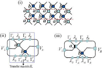
Figure 9: (color online) Key ingredients in the diagonal contraction scheme for obtaining the gradient of the fidelity between a given ground state wavefunction $|\psi\rangle$ and a separable state $|\phi\rangle$ in the iPEPS representation. (i) Tensor network representation for the fidelity between a quantum wavefunction $|\psi\rangle$ and a separable state $|\phi\rangle$. (ii) Tensor network representation for a zero-dimensional transfer matrix $E_{0}$ and its dominant eigenvectors $V_{L}$ and $V_{R}$. Here the infinite matrix product state representation of the dominant eigenvectors for the one-dimensional transfer matrix $E_{1}$ follows from Ref. rosgv , and $V_{L}$ and $V_{R}$ are evaluated using the Lanczos method. The contraction of the entire tensor network is the dominant eigenvalue $\eta_{\langle\phi|\psi\rangle}$ of the zero-dimensional transfer matrix $E_{0}$ for $\langle\phi|\psi\rangle$. (iii) The pictorial representation of the contributions to the derivative of $\eta_{\langle\phi|\psi\rangle}$ with respect to $\tilde{A}^{s*}$, with different relative positions between filled circles and half-filled squares.

Appendix  B Efficient computation of the GE in the iPEPS representation

Once the iPEPS representation for the ground state wavefunction is generated, we are ready to evaluate the GE per lattice site. Here we begin by outlining the scheme developed in Ref. gehlw .

First, we need to compute the fidelity between the ground state wavefunction and a separable state. The latter is represented in terms of one-index tensors $\tilde{A}^{s}$ and $\tilde{B}^{s}$. To this end, we form a reduced four-index tensor $a_{lrud}$ from the five-index tensor $A^{s}_{lrud}$ and a one-index tensor $\tilde{A}^{s}$, as depicted in Fig. 7(iii). As such, the fidelity is represented as a tensor network in terms of the reduced tensors $a_{lrud}$ and $b_{lrud}$ (cf. Fig. 7(iv)).

The tensor network may be contracted as follows. First, form the 1D transfer matrix $E_{1}$, consisting of two consecutive rows of the tensors in the checkerboard tensor network. This is highlighted in Fig. 7(vi) by the two dashed lines. Second, compute the dominant eigenvectors of the transfer matrix $E_{1}$, corresponding to the dominant eigenvalue. This can be done, following a procedure described in Ref. rosgv . Here, the dominant eigenvectors are represented in the infinite matrix product states. Third, choose the zero-dimensional transfer matrix $E_{0}$ (Fig. 8(ii)), and compute its dominant left and right eigenvectors, $V_{L}$ and $V_{R}$. This may be achieved by means of the Lanczos method. In addition, one also needs to compute the norms of the ground state wavefunction $|\psi\rangle$ and a separable state $|\phi\rangle$ from their iPEPS representations. Putting everything together, we are able to obtain the fidelity per unit cell between the ground state $|\psi\rangle$ and a separable state $|\phi\rangle$:

$$\lambda=\frac{|\eta_{\langle\phi|\psi\rangle}|}{\sqrt{\eta_{\langle\psi|\psi\rangle}\eta_{\langle\phi|\phi\rangle}}},$$ (12)

where $\eta_{\langle\phi|\psi\rangle}$, $\eta_{\langle\phi|\phi\rangle}$ and $\eta_{\langle\phi|\phi\rangle}$ are, respectively, the dominant eigenvalue of the zero-dimensional transfer matrix $E_{0}$ for the iPEPS representation of $\langle\phi|\psi\rangle$, $\langle\psi|\psi\rangle$ and $\langle\phi|\phi\rangle$.

We then proceed to compute the GE per site, which involves the optimization over all the separable states. For our purpose, we define $F=\lambda^{2}$. The optimization amounts to computing the logarithmic derivative of $F$ with respect to $\tilde{A}^{*}$, which is expressed as

$$G\equiv\frac{\partial\ln F}{\partial\tilde{A}^{*}}=\frac{1}{\eta_{\langle\phi|\psi\rangle}}\frac{\partial\eta_{\langle\phi|\psi\rangle}}{\partial\tilde{A}^{*}}-\frac{1}{\eta_{\langle\phi|\phi\rangle}}\frac{\partial\eta_{\langle\phi|\phi\rangle}}{\partial\tilde{A}^{*}}.$$ (13)

The problem therefore reduces to the computation of $G$ in the context of the tensor network representation. First, note that a pictorial representation of the derivative $\partial a_{lrud}/\partial\tilde{A}^{s*}$ of the four-index tensor $a_{lrud}$ with respect to $\tilde{A}^{s*}$ is shown in Fig. 8(ii), which is nothing but the five-index tensor $A^{s}_{lrud}$. Similarly, we may define the derivative of the four-index tensor $b_{lrud}$ with respect to $\tilde{B}^{s*}$. Then, we are able to represent the contributions to the derivative of $\eta_{\langle\phi|\psi\rangle}$ with respect to $\tilde{A}^{s*}$ in Fig. 8(iii) and Fig. 8(iv). In our scheme, we update the real and imaginary parts of $\tilde{A}^{s}$ separately:

$$\Re(\tilde{A}^{s}) = \Re(\tilde{A}^{s})+\delta\Re(G)^{s},$$

$$\Im(\tilde{A}^{s}) = \Im(\tilde{A}^{s})+\delta\Im(G)^{s}.$$

Here $\delta\in[0,1)$ is the step size in the parameter space, which is tuned to be decreasing during the optimization process. In addition, we have normalized the real and imaginary parts of the gradient $G$ so that their respective largest entries are unity. The procedure to update the tensor $\tilde{B}^{s}$ is the same. If the fidelity per unit cell converges, then the closest separable state $|\phi\rangle$ is achieved, thus the geometric entanglement per lattice site for the ground state wavefunction $|\psi\rangle$ follows.

The above scheme has some basic limitations for the practical calculation of the GE per site. In particular, it can only be readily achieved for relatively small truncation dimensions. Larger truncation dimensions can be achieved by changing the transfer matrix direction in Fig. 7(vi) to the diagonal direction, as shown in Fig. 9(i). This leads to a simpler calculation of the derivatives necessary for the calculation of the GE (see Fig. 9(ii) and Fig. 9(iii)). For both schemes, the leading computational time scale during contraction is the same, namely $O(D^{4})$. However, in the diagonal scheme, the computation time scale relative to truncation dimension $D$ can be reduced. For example, to calculate the largest eigenvalue $\eta_{\langle\phi|\psi\rangle}$ of $E_{0}$ the computation time for each Lanczos step can be reduced from $O(D^{4})$ to $O(D^{2})$ by storing tensors whose computation time scales as $O(D^{4})$. Since the time cost to obtain $\eta_{\langle\phi|\psi\rangle}$ is mainly due to iterations in the Lanczos algorithm, this improvement allows us to deal with relatively larger truncation dimensions and thus obtain higher accuracy for the GE per site.

References

- (1) For a review, see L. Amico, R. Fazio, A. Osterloh and V. Vedral, Rev. Mod. Phys. 80, 517 (2008).
- (2) H. Barnum and N. Linden, J. Phys. A 34, 6787 (2001).
- (3) T.-C. Wei and P. M. Goldbart, Phys. Rev. A 68, 042307 (2003).
- (4) T.-C. Wei, D. Das, S. Mukhopadyay, S. Vishveshwara and P.M. Goldbart, Phys. Rev. A 71, 060305 (2005).
- (5) R. Orús and T.-C. Wei, Phys. Rev. B 82, 155120 (2010); R. Orús and T.-C. Wei, Quantum Inf. Comput. 11, 0563 (2011); R. Orús, T.-C. Wei and H.-H. Tu, Phys. Rev. B 84, 064409 (2011).
- (6) A. Botero and B. Reznik, arXiv:0708.3391.
- (7) R. Orús, Phys. Rev. Lett. 100, 130502 (2008).
- (8) Q.-Q. Shi, R. Orús, J. O. Fjærestad, and H.-Q Zhou, New J. Phys. 12, 025008 (2010).
- (9) J.-M. Stéphan, G. Misguich and F. Alet, Phys. Rev. B 82, 180406R (2010).
- (10) B.-Q. Hu, X.-J. Liu, J.-H. Liu and H.-Q. Zhou, New J. Phys. 13, 093041 (2011).
- (11) I. Affleck and A.W.W. Ludwig, Phys. Rev. Lett. 67, 161 (1991).
- (12) R. Orús, S. Dusuel and J. Vidal, Phys. Rev. Lett. 101, 025701 (2008).
- (13) C.-Y. Huang and F.-L. Lin, Phys. Rev. A 81, 032304 (2010).
- (14) H.-L. Wang, Q.-Q. Shi, S.-H. Li and H.-Q. Zhou, arXiv:1106.2129.
- (15) J. Jordan, Studies of Infinite Two-Dimensional Quantum Lattice Systems with Projected Entangled Pair States, PhD Thesis, University of Queensland (2011) http://www.romanorus.com/JordanThesis.pdf
- (16) R. Orús, T.-C. Wei, O. Buerschaper and A. Garcia-Saez, Phys. Rev. Lett. 113, 257202 (2014).
- (17) R. Mohseninia, S. S. Jahromi, L. Memarzaeh and V. Karimipour, Phys. Rev. B 91, 245110 (2015).
- (18) L. M. Ionnou, Quantum Inf. Comput. 7, 335 (2007).
- (19) L. Huang, New J. Phys. 16, 033027 (2014).
- (20) F. Verstraete, D. Porras, and J. I. Cirac, Phys. Rev. Lett. 93, 227205 (2004); F. Verstraete and J. I. Cirac, arXiv:cond-mat/0407066; V. Murg, F. Verstaete and J. I. Cirac, Phys. Rev. A 75, 033605 (2007).
- (21) G. Vidal, Phys. Rev. Lett. 91, 147902 (2003); 93, 040502 (2004); 98, 070201 (2007).
- (22) J. Jordan, R. Orús, G. Vidal, F. Verstraete and J. I. Cirac, Phys. Rev. Lett. 101, 250602 (2008).
- (23) H. C. Jiang, Z. Y. Weng and T. Xiang, Phys. Rev. Lett. 101, 090603 (2008).
- (24) B. Bauer, G. Vidal and M. Troyer, J. Stat. Mech. P09006(2009).
- (25) R. Orús and G. Vidal, Phys. Rev, B 78, 155117 (2008).
- (26) P. Pippan, S. R. White and H. G. Evertz, Phys. Rev. B 81, 081103(R) (2010).
- (27) Q.-Q. Shi and H.-Q. Zhou, J. Phys. A 42 272002 (2009).
- (28) J. Haegeman, J. I. Cirac and T. J. Osborne, I. Pižorn, H. Verschelde and F. Verstraete, Phys. Rev. Lett. 107, 070601 (2011).
- (29) L. Wang, Y.-J. Kao and A.W. Sandvik, Phys. Rev. E 83, 056703 (2011).
- (30) For recent reviews, see R. Orús, Ann. Phys. (N.Y.) 349, 117 (2014); Eur. Phys. J. B 87, 280 (2014).
- (31) H. N. Phien, J. A. Bengua, H. D. Tuan, P. Corboz and R. Orús, Phys. Rev. B 92, 035142 (2015).
- (32) H.-Q. Zhou and J. P. Barjaktarevi, J. Phys. A 41, 412001 (2008); H.-Q. Zhou, J.-H. Zhao and B. Li, J. Phys. A 41, 492002 (2008).
- (33) H.-Q. Zhou, R. Orús and G. Vidal, Phys. Rev. Lett. 100, 080602 (2008).
- (34) B. Li, S.-H. Li and H.-Q. Zhou, Phys. Rev. E 79, 060101(R) (2009).
- (35) J.-H. Zhao, H.-L. Wang, B. Li and H.-Q. Zhou, arXiv:0902.1669; Phys. Rev. E. 82, 061127 (2010).
- (36) H.-L. Wang, J.-H. Zhao, B. Li and H.-Q. Zhou, J. Stat. Mech. L10001(2011).
- (37) F-Y. Wu, Rev. Mod. Phys. 54, 235 (1982).
- (38) Y.-W. Dai, S. Y. Cho, M. T. Batchelor and H.-Q. Zhou, Phys. Rev. E 89, 062142 (2014).
- (39) The result for can be compared with previous estimates. For a special direction of the field, the toric code in a magnetic field corresponds to the -state quantum Potts model in a transverse field. This model was studied using iPEPS toric to compute the critical field value for . Note also from series expansion series , one gets . These results are to be compared with our estimate of . We thank Julien Vidal for these remarks.
- (40) M. D. Schulz, S. Dusuel, R. Orús, J. Vidal and K. P. Schmidt, New J. Phys. 14, 025005 (2012).
- (41) C. J. Hamer, J. Oitmaa and Z. Weihong, J. Phys. A 25, 1821 (1992).
- (42) J. Solyom and P. Pfeuty, Phys. Rev. B 24, 218 (1981).
- (43) See, e.g., A. W. Sandvik, AIP Conf. Proc. 1297, 135 (2010) and references therein.
- (44) N. D. Mermin and H. Wagner, Phys. Rev. Lett. 17, 1133 (1966).
- (45) J. D. Reger and A. P. Young, Phys. Rev. B 37, 5978 (1988); A. W. Sandvik and H. G. Evertz, Phys. Rev. B 82, 024407 (2010);
- (46) T. Roscilde, P. Verrucchi, A. Fubini, S. Haas and V. Tognetti, Phys. Rev. Lett. 94, 147208 (2005).
- (47) H.-Q. Lin and V. J. Emery, Phys. Rev. B 40, 2730 (1989); R. F. Bishop, J. B. Parkinson and Y. Xian, Phys. Rev. B 46, 880 (1992); V. Y. Irkhin, A. A. Katanin and M.I. Katsnelson, J. Phys.:Condens. Matter 4, 5227 (1992); D. J. J. Farnell, K. A. Gernoth and R. F. Bishop, Phys. Rev. B 64, 172409 (2001).
- (48) A. Chandran, V. Khemani and S. L. Sondhi, Phys. Rev. Lett. 113, 060501 (2014).