Scattering of gravity waves in subcritical flows over an obstacle
Abstract
We numerically study the scattering coefficients of linear water waves on stationary flows above a localized obstacle. We compare the scattering on trans- and subcritical flows, and then focus on the latter which have been used in recent analog gravity experiments. The main difference concerns the magnitude of the mode amplification: whereas transcritical flows display a large amplification (which is generally in good agreement with the Hawking prediction), this effect is heavily suppressed in subcritical flows. This is due to the transmission across the obstacle for frequencies less than some critical value. As a result, subcritical flows display high- and low-frequency behaviors separated by a narrow band around the critical frequency. In the low-frequency regime, transmission of long wavelengths is accompanied by non-adiabatic scattering into short wavelengths, whose spectrum is approximately linear in frequency. By contrast, in the high-frequency regime, no simple description seems to exist. In particular, for obstacles similar to those recently used, we observe that the upstream slope still affects the scattering on the downstream side because of some residual transmission.
pacs:
04.60.-m, 04.62.+v, 04.70.Dy, 47.35.BbI Introduction
In 1981, Unruh pointed out that one might conceive of experiments where the analog version of black hole radiation could be observed in a moving medium Unruh (1981). Indeed, when the flow is stationary and transcritical, i.e., when the flow speed crosses the wave velocity, the propagation of linear density perturbations is governed by an equation which has the form of a d’Alembertian in a black hole geometry. As a result, the scattering coefficients should be identical to those encoding the Hawking effect. However, it was then realized that this ceases to be exact when taking into account the dispersive effects that occur at short wavelengths in condensed matter media Jacobson (1991); Unruh (1995).
As a result, to be able to predict what should be seen in experiments, one should compute the scattering coefficients taking into account the specific dispersive effects characterizing the medium. It was first understood that the spectrum is robust Unruh (1995); Brout et al. (1995); Corley and Jacobson (1996); Corley (1998); Unruh and Schutzhold (2005); Balbinot et al. (2005), i.e., that the spectral deviations from the standard thermal distribution are suppressed by positive powers of , where and are respectively the analog version of the surface gravity and the dispersive scale above which dispersion effects are significant. Hence when , the emitted spectrum closely follows a Planck distribution with a temperature given by in units . When is not negligible, the spectrum is no longer Planckian Macher and Parentani (2009a, b), yet its main properties can be understood in terms of two parameters: and a critical high frequency , which is linearly related to but which also depends on the parameters of the background flow Finazzi and Parentani (2012). In particular, there is a smooth transition from the standard relativistic regime , to a dispersive regime where no longer plays any role. It is fair to say that the scattering coefficients in transcritical flows are now well understood, see Robertson (2012); Coutant et al. (2012a) for reviews.
When considering the experiments based on surface waves in water tanks Rousseaux et al. (2008, 2010); Weinfurtner et al. (2011); Euvé et al. (2015a, b), one encounters two novel effects. Firstly, the background flows investigated up to now have been subcritical rather than transcritical. Since there is no analog Killing horizon in such flows, the link with the Hawking effect is a priori unclear. In fact, the spectral properties are not well understood, and have so far received much less attention than their counterparts in transcritical flows. Preliminary studies indicate that several regimes are found, and that various parameters are relevant in each regime Michel and Parentani (2014, 2015); Coutant and Weinfurtner (2016). Secondly, downstream from the obstacle, the free surface is modulated by a zero-frequency undulation with a macroscopic amplitude and a long extension Lawrence (1987); Coutant and Parentani (2014). Typically, the undulation is longer than a meter and its amplitude is of the order of cm, larger that the typical amplitude of the waves sent by the wavemaker which is of the order of a few mm. The extra scattering on such an extended modulation is poorly understood. Numerical simulations indicate that it might play a significant role in experiments Euvé et al. (2015b), see also Busch et al. (2014) for a study in the context of atomic Bose-Einstein condensates.
We shall study these two aspects in turn. In this first paper, we focus on the scattering coefficients in subcritical flows with no undulation downstream from the obstacle. Our principal aim is to characterize the main properties of these coefficients, and to show how they depend on the background flow parameters. We hope our predictions can be tested in forthcoming experiments. In a future paper we shall study the scattering on the undulation itself.
The present work is organized as follows. In Sec. II we present the simplified wave equation for linear perturbations and the particular parametrization of background flows over an obstacle used in our analysis. Then, we identify the four modes involved in the scattering, and compare the behaviors of the 16 scattering coefficients in a typical transcritical and a subcritical flow. We end the section by studying the evolution of the scattering coefficients when gradually replacing a transcritical flow by a subcritical one. In Sec. III we focus on sub- and near-critical flows. We show that the scattering on such flows should be analyzed separately in three different frequency regimes, in each of which we identify the relevant flow parameters. We conclude in Sec. IV. In Appendix A we show how the three regimes appear when studying the effective temperature as a function of the upstream and downstream slopes of the flow, and in Appendix B we examine more closely the respective roles played by these two slopes when the flow is asymmetrical.
II Scattering in trans- and subcritical flows
II.1 The simplified wave equation
We shall study linear surface waves propagating in inhomogeneous flows of an ideal, inviscid, incompressible fluid. Following Schutzhold and Unruh (2002); Unruh (2013); Michel and Parentani (2014) the flows are assumed to be stationary, irrotational, and laminar. We assume they take place in an elongated flume and neglect any dependence on the directions orthogonal to the mean velocity. In addition, we neglect capillary effects, which means that the wavelengths we consider are significantly larger that the typical capillary length ( a few mm for water). Finally, we assume that the inhomogeneity of the flow is due to an obstacle put on the bottom of the flume.
Under these assumptions and considering waves which are homogeneous in the transverse direction, the dispersion relation between the (conserved) angular frequency and the wave number in the longitudinal direction is
| (1) |
where is the horizontal flow velocity, the water depth, and the gravitational acceleration. In inhomogeneous flows, , , , and depend on , the position in the longitudinal direction. The quantity gives the frequency in the frame co-moving with the fluid. Although it is not constant, its sign plays a crucial role in the analysis of the scattering.
Despite the simplicity of Eq. (1), the linear equation governing the propagation of waves is rather complicated. The explicit expression can be found in Unruh (2013); Coutant and Parentani (2014). In particular, because of the term in , it contains operators with arbitrarily high orders of . To simplify the numerical resolution, as in Michel and Parentani (2014); Euvé et al. (2015a); Michel and Parentani (2015), we consider a quartic truncation of this equation keeping the ordering of , and . Namely, we work with
| (2) |
where is the perturbation of the velocity potential. It is related to the linear variation of the water depth through
| (3) |
The truncated dispersion relation associated with Eq. (2) is
| (4) |
In the hydrodynamical limit , the (local value of the) speed of propagation of shallow waves becomes .
When the Froude number is close to 1, Eq. (2) becomes equivalent to the full wave equation in the range of frequencies we are interested in. It is thus sufficient to characterize the main properties of the scattering for near-critical flows. We refer to Coutant et al. (2012a) for an analytical calculation of the scattering coefficients based on Eq. (2) when the flow is transcritical. In these flows, the link with the Hawking effect, and the first deviations due to dispersion, are both clear. For the low frequency behavior in subcritical flows, we refer to Coutant and Weinfurtner (2016) which appeared while we were finishing the present work.
Eq. (2) has a conserved scalar product with the same structure as that of the complete equation. It is given by
| (5) |
where and are two complex solutions. We refer to Coutant and Parentani (2014) for the relation between Eq. (5) and the wave energy, and for the fact that the norm is not positive definite. In fact, the sign of the norm is that of , the frequency in the co-moving frame (see Eq. (1)). 111 The conservation of the norm should not be confused with that of the wave action Bretherton and Garrett (1968), although these notions are closely related. While the former is exact, the conservation of the wave action is an approximate (adiabatic) law which only applies to flows with low temporal and spatial gradients. The link is clear when restricting attention to stationary inhomogeneous flows. In this case, the validity of the WKB approximation of Eq. (2), see Coutant and Parentani (2014), guarantees that the wave action is constant. Considering a stationary mode solution of Eq. (2), the wave action is given by where , , and , see Eq. (3). The scattering coefficients we shall compute encode non-adiabatic effects Massar and Parentani (1998); Coutant and Weinfurtner (2016), i.e., violations of the conservation of the wave action.
II.2 The parametrization of inhomogeneous flows
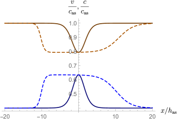
Assuming the flow is homogeneous in the vertical direction, the local low-frequency wave speed and background flow velocity are respectively given by and , where is the conserved water current. The local value of the Froude number is thus
| (6) |
In this paper, we work with , that is, the flow goes from left to right. We phenomenologically describe the properties of the flow on top of a localized obstacle using the following parametrization of : 222An alternative approach would be to consider background flows that are solutions of the hydrodynamical equations over known obstacles. This approach has been presented in Appendix A of Michel and Parentani (2014). We verified that the behavior of the scattering coefficients is similar to that presented here.
| (7) |
where
| (8) |
The constant is chosen so that , and the parameters , , and are strictly positive. is the maximum value of reached on top of the obstacle, see fig. 1. is its asymptotic value, and is smaller than 1 so that the flows we consider are all asymptotically subcritical. By analogy with the transcritical case where crosses , we will often refer to the upstream slope () as the black hole, and to the downstream slope () as the white hole (even though there is no analogue Killing horizon if ).
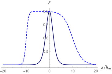
When is smaller than or of the same order as , , , and do not individually give accurate estimations of the length and slopes of the obstacle. It will thus be convenient to define effective values in the following way. We call (resp. ) the value of where (resp. ) is largest. For large values of , one obtains , but these can differ significantly for smaller lengths, see fig. 1. We thus define the effective length and slopes by
| (9) |
It should be noticed that Eqs. (7) and (8) involve only dimensionless quantities when expressing , , , and in units of the asymptotic water depth . As a result, each set of parameters effectively corresponds to a one-parameter family of water depth profiles related to each other by a rescaling of all lengths. Moreover, this transformation does not change the behavior of the scattering coefficients. Indeed, the non-linear fluid equations Unruh (2013); Coutant and Parentani (2014) contain only one dimensionful parameter when surface tension and viscosity are neglected: the gravitational acceleration . They are thus invariant under multiplication of all lengths by a positive number and all times by . This implies that the scattering coefficients extracted from the linear wave equation (2) are also left invariant.
II.3 The -matrix
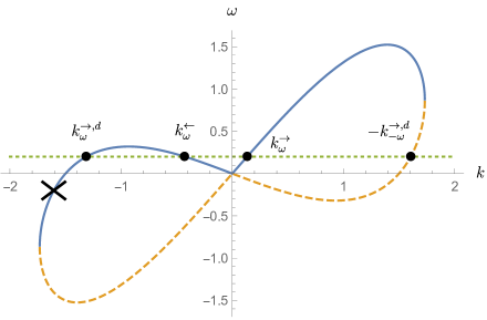
Since Eq. (2) does not depend explicitly on time, one can decompose any solution in terms of modes with fixed angular frequency . Moreover, in the asymptotic regions where is constant, these stationary modes are superpositions of plane waves , where is related to by Eq. (4). In the present work, we only consider frequencies in the interval , where is the frequency at which two roots in the upper left quadrant of fig. 2 merge (at Froude number equal to its asymptotic value ). Using the quartic dispersion relation of Eq. (4), and , it is given by
| (10) | |||||
where the second equation is valid for , for more details we refer to Eqs. (9) and (10) of Michel and Parentani (2014). In the domain , there are four real roots of Eq. (4), and thus four plane waves satisfying Eq. (2). Explicitly, these are the following:
- •
-
•
is a dispersive mode (in that its wave vector does not vanish when ) and right-moving.
-
•
is also dispersive and right-moving.
-
•
is hydrodynamic and right-moving.
The third mode has been complex-conjugated because its norm is negative, see Eq. (5), while the other three modes have positive norms. We adopt the standard notation such that all modes without complex conjugation have scalar product , and hence, according to the definition (5), the complex conjugated modes have scalar product . It should be noticed that carries a negative energy. Hence, when increasing the amplitude of this mode, the wave energy is reduced, see Coutant and Parentani (2014) for more details. The arrow in the superscript gives the sign of the group velocity in the laboratory frame, i.e., the sign of . The first 3 modes are counter-propagating with respect to the fluid. In transcritical flows, their mixing through scattering on the obstacle encodes the analog Hawking effect Unruh (1995); Brout et al. (1995). The last mode instead is co-propagating (with respect to the fluid) and plays no significant role in this regard. In fact, to obtain a good analogy with the standard Hawking prediction, one should minimize the coefficients governing its mixing with the three other modes Macher and Parentani (2009a); Busch and Parentani (2014).
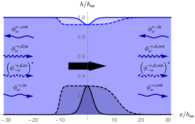
We now consider two bases of globally defined modes, that is, solutions of Eq. (2) defined for all . The in basis contains four modes with only one incoming wave, i.e., one asymptotic wave with group velocity oriented towards the horizon. Similarly, the out basis comprises those modes with only one outgoing wave. The aim of the present work is to determine numerically the properties of the scattering matrix relating these two bases. We shall denote by a superscript “” (resp. “”) the in (resp. out) modes, so that, for instance, is the (global) mode which asymptotically contains only as incoming wave.
Generalizing the notation used for the -matrix of Ref. Macher and Parentani (2009a), we write the relationship between the two bases as
| (11) |
The superscript has been added to ease the identification of the coefficients involving the co-propagating mode . The -matrix is an element of . This is a direct consequence of the fact that the scalar product of Eq. (5) is conserved, and that the norm of is the opposite of that of the three other modes. As a result, the squared absolute values of the coefficients of the first line satisfy
| (12) |
(When the transmission and the reflection channels can be neglected, one recovers the standard mode mixing which gives .) Similar equations apply to the other lines, and to the columns. In these 8 relations, the squared absolute values of the 4 coefficients and the 2 coefficients are all multiplied by a minus sign. These 6 coefficients encode some mode amplification compensated for by excitation of the negative energy mode.
II.4 The behavior of the 16 scattering coefficients
II.4.1 Transcritical flows
To prepare the analysis of the scattering in subcritical flows, we first show how the 16 coefficients of Eq. (11) behave in a transcritical flow with and . For simplicity, we choose a symmetric flow. We also choose to work with a narrow obstacle, as this eases the observation of the transmission occuring at very low frequency. Explicitly, we work with and . Since the flow is transcritical it has two analog horizons where . The analog Hawking temperature evaluated on the horizons is . To give an example, if one chooses , the white (black) hole horizon is at , and .
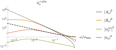
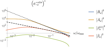
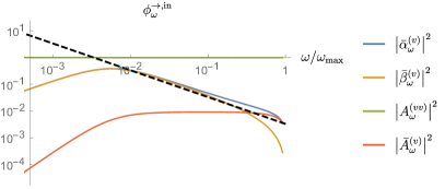
In each panel of fig. 4, as a function of , we represent in log-log plots the squared absolute values of the four coefficients when sending each of the incoming waves of the left-hand side of Eq. (11). The symbol of the incoming mode is given on top of the panel, while each color always indicates the same outgoing mode, namely blue for , orange for , green for the co-propagating mode , and red for .
The most important observation is that the absolute values of some scattering coefficients are significantly larger than 1. This indicates that the mode amplification (pair creation in quantum terms) induced by the scattering on this transcritical flow is large. Since the Hawking prediction is , one should look for curves which grow like for .
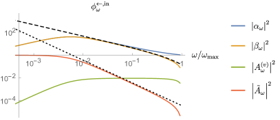
On the first panel, when sending from the downstream right side, this growth characterizes the modes and . This is to be expected from the Hawking radiation taking place in a white hole flow: in this case, the outgoing radiation is carried by the two dispersive modes emitted on the same side of the horizon. To show the quality of the agreement between the numerical outcome and the Hawking spectrum, the dotted black line follows the Planck law with the temperature evaluated on the white hole horizon. We can see that the agreement is excellent in a wide domain of frequencies containing even though we work in a rather dispersive regime since Finazzi and Parentani (2012). The upper limit of the domain is near , while its lower limit where the growth stops is here . This is due to the transmission across the obstacle of ultra low-frequency modes. In fact, in the ultra low-frequency regime, we notice that and agree with each other, and decrease linearly in for . As a result, the zero-frequency limit is fully characterized by the frequency defined by
| (13) |
The critical frequency is then given by . This simple relation follows from matching the two behaviors of above and below , namely and , respectively. When working in the limit of steep slopes, an approximate expression for is
| (14) |
see Eq. (20) of Michel and Parentani (2014). Here is the imaginary part of the root of the dispersion relation at in the upper complex plane. In the present flow, one gets . Equation (14) gives a reliable estimation of for sufficiently long obstacles, i.e. for . We shall see in Sec. III that the damping of the evanescent mode also plays a crucial role in the characterization of subcritical flows.
On the second panel, when sending the short wavelength mode from the left side, one observes that the growth in characterizes the mode in red, as expected from the Hawking effect taking place on the black hole side. To underline the agreement the dashed black line here follows the theoretical prediction . Again the agreement is excellent down to the low-frequency cut-off where the growth stops. We also notice the presence of two curves which grow like . This behavior is indicated by a dotted straight line which gives . This growth is due to the fact that these modes have been scattered on both horizons. As a result their scattering coefficients essentially grow like the product of the amplification associated with each horizon, as was discussed in Coutant et al. (2012b). The same observations apply to the first two coefficients of the third plot which are obtained when sending the dispersive negative norm mode from the left. On the third panel, we also see that the mode in red closely follows the Planck law indicated by a dashed line.
On the last panel, irrespective of the frequency, we see that the co-propagating mode is essentially transmitted. This indicates that the mode nearly decouples from the three other modes, which are counter-propagating with respect to the fluid. In addition, when considering the green curves on the three other panels, one verifies that their values are always subdominant. These observations establish that (in transcritical flows at least) the scattering coefficients involving the co-propagating mode can be neglected, to a good approximation.
II.4.2 Subcritical flows
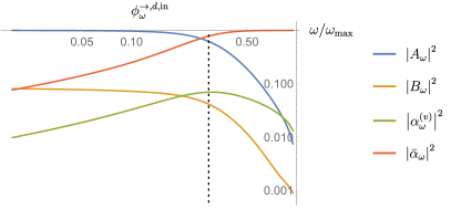
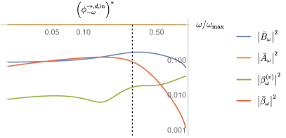
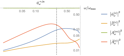
We now consider the scattering coefficients in a subcritical flow with , , and . The effective values of Eq. (9) are , , and . In the four panels of fig. 5, as a function of , we show the log-log plots representing the squared absolute values of the same scattering coefficients as in fig. 4, following the same notational conventions.
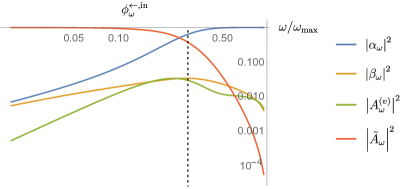
The main difference one immediately sees is that the scattering coefficients are suppressed with respect to the transcritical case, never becoming appreciably larger than 1. This reveals that in subcritical flows there is no significant mode amplification. In other words, the 6 anomalous coefficients mixing modes with opposite norms all remain much smaller than 1. For instance, in the first panel, the squared norm of the coefficient (encoding the scattering on the “white hole” side) is always smaller than . The same observation applies to the coefficient encoding the scattering on the “black hole” side, see the red curve of the third panel. The lesson here is very clear: when the Froude number remains smaller than 1, the typical growth of the coefficients in is no longer found. This could be understood from the absence of any Killing horizon in the associated effective metric Unruh (1981).
The absence of horizons in subcritical flows introduces a new critical frequency, which we shall call , and which is indicated by a vertical line in the four panels of Figure 5. It is the frequency at which the dispersion relation has a double root for , vanishing as . In the quartic approximation of Eq. (4), it is thus given by the same expression of Eq. (10) but now evaluated on top of the obstacle where and reach their minimal values:
| (15) |
For , the two upper panels show that the hydrodynamical mode is blocked and reflected onto the dispersive mode, and vice versa, see the red and blue curves. This can be understood from the fact that the corresponding characteristics have a turning point for Michel and Parentani (2014). Similarly, the absence of significant scattering experienced by the negative norm mode and the co-propagating modes (see the two lower panels) can also be understood from the validity of the WKB approximation for the propagation of both of these modes.
For , the situation is even simpler as the four incident modes are essentially transmitted above the obstacle. In fact, the mode mixing coefficients are all small, as can be understood from the fact that they encode non-adiabatic corrections in a domain where the WKB approximation is reliable Coutant and Weinfurtner (2016). In the limit , the squared norms of the coefficients relating a dispersive mode and a hydrodynamic one go to zero as Michel and Parentani (2014), while those relating the two hydrodynamic modes decrease faster, as . Notice however that and go to non-vanishing values. This behavior is similar to the one found at very low frequency in transcritical flows, although the non-vanishing values are much smaller in subcritical flows because the growth found in fig. 4 is no longer present.
II.5 Evolution of the scattering coefficients of when varying
We observed in the previous subsection that the behavior of the coefficients critically depends on whether the flow is sub- or transcritical. To display the transition between these two behaviors, we gradually lower from to , focussing on the left-moving incoming mode , which is most relevant for the experiments performed in Nice, Vancouver, and Poitiers Rousseaux et al. (2008); Weinfurtner et al. (2011); Euvé et al. (2015a, b). Explicitly, the first line of Eq. (11) gives
| (16) |
where the four scattering coefficients satisfy Eq. (12).
The precise evolution of the scattering coefficients when decreasing depends on the variations of the other flow parameters. Here, we work with fixed values of and , which are the same as those used in fig. 5, while we vary the parameters of Eq. (8) so that the generalized surface gravities
| (17) |
differ by less than when varying from to . Explicitly, the values of and used in fig. 6 are derived from those of fig. 5 by dividing by , so that corresponds to exactly the same flow in both figures.
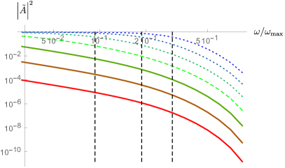
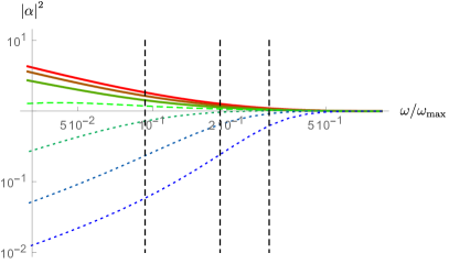
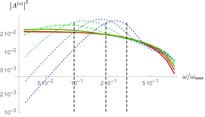
The upper left plot of fig. 6 shows the squared absolute value of the transmission coefficient for 7 flows: three subcritical, one critical () and three transcritical. For the three subcritical flows (dotted curves), for smaller than the corresponding values of which are indicated by three dotted vertical lines, the transmission coefficient is close to 1, i.e., there is no blocking of incident waves. For the critical flow (dotted line), one sees that approaches for low frequency. Instead, for the three transcritical flows, it remains smaller than for the whole frequency range shown in the figure. (Because of the finite size of the obstacle, it nevertheless tends to 1 in the limit .) Interestingly, when increasing at fixed , decreases nearly exponentially in the region where it is small. Correspondingly, the critical frequency of Eq. (14) at which transmission becomes significant increases and becomes of the order of when .
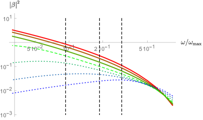
The dichotomy between trans- and subcritical flows is more pronounced when considering the coefficients and . When the flow is significantly transcritical, i.e. , there is a wide frequency domain between and where and are proportional to . This interval shrinks when decreasing and vanishes on reaching the critical case . For all subcritical flows, one clearly sees that and go to zero linearly as Michel and Parentani (2014). As a result, in subcritical flows the maximal value of is reached near , and steadily decreases as is decreased further.
In the lower right panel, for subcritical flows, we notice that decreases as for . In transcritical flows, this decrease can only be seen for frequencies close to or smaller than , leaving a wide interval where is nearly constant, but not significant as .
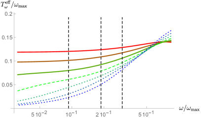
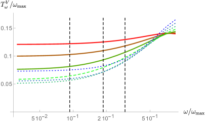
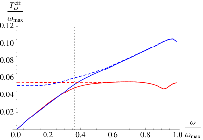
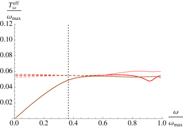
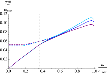
To complete this comparison, it is interesting to study the behaviors of two effective temperatures which have been used to characterize the spectrum. The first one is defined by , i.e.,
| (18) |
Constancy of is equivalent to following the Planck law with temperature , see Macher and Parentani (2009a, b); Finazzi and Parentani (2012). The second one is defined by Weinfurtner et al. (2011)
| (19) |
These coincide whenever . In fig. 7, they are shown as functions of for the same flows as those of fig. 6. In transcritical flows and for , they are both nearly constant and very close to each other, as can be understood from the fact that the transmission and the “gray body” factor are both negligible. In this case, follows from unitarity, see Eq. (12).
However, they strongly differ in subcritical and near-critical flows. (In fact they also differ in transcritical flows but only at very low frequencies, for .) In these cases, goes to zero linearly when because of the aforementioned behavior of , i.e., the suppression of the amplification mechanism at low frequencies due to transmission. On the other hand, approaches a finite value in that limit. This is because and both go to zero linearly, so that their ratio goes to a finite, non-vanishing constant. Interestingly, we notice that this constant value increases when decreasing , as can be seen in the crossing of the dotted lines occurring for in the right plot of fig. 7. Our numerical simulations suggest that it goes to infinity in the limit , i.e., when approaching a homogeneous flow without obstacle.
III Influence of the background flow parameters
Let us now focus our attention on subcritical and near-critical flows. As in Sec. II.5, we again restrict our attention to the left-moving incoming mode of Eq. (16). Our aim is to identify the relevant parameters determining the spectral properties of the scattering coefficients. To this end, we consider three different phenomena characterized by the value of the frequency:
-
•
When increasing near , the scattering of varies from near-total transmission across the obstacle to an essential reflection from the obstacle. More precisely, the transmission coefficient varies from near to near , while varies in the opposite manner. The sharpness of the transition will be quantified by the derivative of at .
-
•
Below , and , the squared absolute values of the coefficients multiplying the dispersive modes in Eq. (16) become close to each other, and both vanish linearly in for .
-
•
Above , so long as the obstacle is sufficiently long that tunnelling effects are negligible, we expect only the flow properties in the downstream (white hole) region to be relevant, just as if the flow were transcritical. It is in this frequency domain that one could hope to obtain a close relationship with the Hawking predictions. For narrow obstacles, however, the behavior in this regime can be rather complicated.
In Appendix A, it can be seen that these three behaviors are clearly present when considering the effective temperature of Eq. (18) in the -plane. Here, we shall look separately at the three scenarios delineated above, picking out the relevant parameters of the flow which determine the main behavior of the scattering coefficients in each case.
III.1 Transition near
For , the characteristics for the left-moving incident mode are blocked: there is a turning point they cannot pass, instead continuously evolving into right-moving characteristics of the outgoing dispersive mode Michel and Parentani (2014). An entirely analogous blocking occurs for the right-moving incident mode from the left side, which continuously evolves into the left-moving outgoing mode . By contrast, for , no such blocking occurs, and the characteristics of both modes traverse the obstacle. There is thus a significant change in behavior at , quite independent of the analogue Hawking effect, involving only the scattering coefficients and of Eq. (16). We shall consider , and define the dimensionless parameter
| (20) |
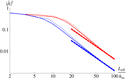
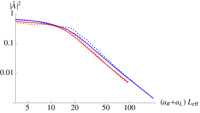
In Figure 8 is shown the transmission coefficient evaluated at for a variety of flows, with particular emphasis on how it depends on the adimensionalised effective length of the obstacle. For obstacles which are narrow enough, is approximately constant and close to , so that marks the midpoint of the transition. However, for longer obstacles, scales as . We can make sense of this by noting that, in the limit where becomes infinite and we are left with a single horizon, there can be no transmission at all for , so to maintain continuity of the scattering coefficients we must have going to zero in this limit. Figure 8 also indicates that the effects of the slope can be approximately accounted for by using as the variable rather than . (See Eq. (8) for the definition of .) Finally, fig. 8 shows that has little bearing on , as was observed in Ref. Euvé et al. (2015a).


In Figure 9 are shown plots of the adimensionalised derivative of Eq. (20) for several different values of . In the left panel, is varied while is fixed at , the adimensionalized effective length is fixed at , and is fixed at . We see that, while there is a dependence on the slope , this is not as important as the dependence on , with being systematically reduced as is increased. In the right panel, is varied while , and . We see there that is an important quantity in determining when both are relatively small. Indeed, when increasing from to , is seen to increase by a factor of between and , depending on the value of . At large , however, shows only small oscillations around some -dependent limiting value. Notice also that, unlike at small , the dependence on is non-monotonic at large .
There is a clear lesson here in the case of relatively narrow obstacles (i.e. ). According to Figure 8, the critical frequency corresponds more or less to the midpoint of the transition region, and hence (which is defined at ) serves as a good indication of the sharpness of the transition. Turning to Figure 9, we find that in this regime, the sharpness of the transition increases with increasing and decreases with increasing , while it is essentially independent of . The dependence on is particularly intuitive: the narrower the obstacle, the higher will be the rate of tunnelling across it, and so we need higher frequencies with more rapidly decaying evanescent modes in order to find a mode which is truly blocked. It is less clear how to interpret the results for large , for then is no longer measured at the midpoint of the transition.
III.2 Low-frequency regime
For , there are no turning points according to geometrical optics, so that the incident wave is essentially transmitted, i.e., . This is clearly seen in the top left panel of Figure 5. Furthermore, the same panel reveals that for , in accordance with Eq. (13).
To characterize the zero-frequency limit, we study how the frequency depends on the flow parameters.


In Figure 10 is plotted as a function of the downstream slope , with fixed values of , and . The various curves correspond to different values of , which we allow to vary from a subcritical to a supercritical value. We note that, although there is a clear dependence on the slope , this is subdominant with respect to the dependence on , whose effect is much greater. 333An exception to this is the peak in the curve centred around . This is a resonant behavior in due to the symmetry of the flow profile. The rapid decrease of with increasing can be understood from the results presented in Figure 4: when the flow is transcritical, the scattering coefficients and first increase as in some interval, in stark contrast to the linear behavior seen in the subcritical case. Interpolating between these two different behaviors requires that decrease when increasing , and indeed the window of validity of the linear behavior of Eq. (13) must shrink accordingly. It does not vanish when reaches 1, however; we recall from Figure 4 that there exists an ultra-low frequency regime where tunnelling across the obstacle is significant, and where even for transcritical flows. This allows to be well-defined even when .
To further investigate the behavior of with as the latter approaches , we fixed the values of and at and , respectively, and plotted for varying and . The results are shown in Figure 11. Firstly, we notice that does not vanish as but approaches a finite value, which decreases with increasing . In this regime, has taken over as the relevant parameter. Secondly, there is an interesting change of behaviour at , a changeover point which is seemingly independent of . For larger than this value, the curves converge to one which is proportional to , with only the curve for the smallest value of showing significant deviations from the others. In this regime, then, and so long as is not too small, is the only relevant parameter in determining . Finally, we note that there is also an intermediate regime where both and are relevant parameters. In this third regime, there are significant oscillations in with a period that depends on . Interestingly, the troughs of these oscillations all follow a curve which is proportional to (or , according to Eq. (15)). 444While completing our numerical analysis, we became aware of Coutant and Weinfurtner (2016) where the low-frequency regime is investigated in analytical terms. We performed a few extra simulations which indicate good agreement with numerical integration of their Eq. (B10). On the other hand, it is presently unclear to us if the various behaviors displayed in our Fig. 11 can be recovered from their Eq. (B14). We are thankful to Antonin Coutant for explanations about the expected validity domain of the equations of Coutant and Weinfurtner (2016).
From an experimental perspective, however, it is quite unlikely for to be so close to that we find ourselves in the region of Figure 11 where plays a significant role. Generally speaking, then, and up to the possibility of resonant effects, is by far the most relevant quantity in the determination of , the latter decreasing rapidly as approaches . Sufficiently narrow obstacles constitute an exception, as we can begin to see from the (dotted) curve of Fig. 11. But this effect is subdominant relative to the dependence on .
III.3 High-frequency regime
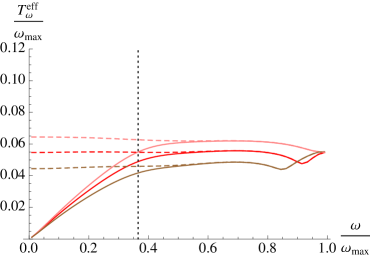
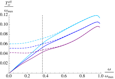
It turns out that the high-frequency regime is the most complicated to describe. For, while we might naively expect the spectrum here to be approximately thermal (since the wave is blocked much as in the transcritical case), it appears that this is only sometimes true. As we shall see, the difficulties come in part from the residual transmission across the obstacle. To get a flavor of the behavior in this regime, we shall study here the spectrum on a series of flows obtained by fixing one of the two slopes and letting the other vary. We shall examine the behavior of both , the effective temperature at the mid-point of the high-frequency regime, i.e., at , and of its derivative evaluated at the same frequency. The latter quantity is very important in that it quantifies (at least approximately) the variation of the effective temperature, and thus the Planckianity of the spectrum, see Eq. (18).
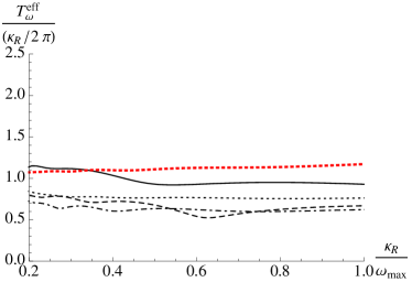

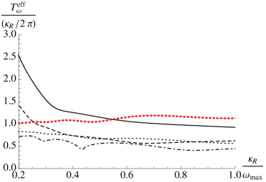
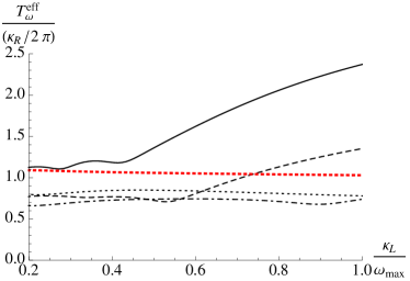
Illustrative examples of these two quantities are shown in Figure 12. Note that has been normalized by , a generalized version of the Hawking temperature, so that what is plotted in all but the upper right plot is in effect the “Hawkingness” of the spectrum at the midpoint frequency. In the top row, is held fixed at and is varied, so that the flow has a small upstream slope. The normalized effective temperature is shown on the left and the derivative of the temperature is shown on the right. In the bottom row, the normalized effective temperature is shown for two series of flows which exhibit significant deviations from the Hawking-like prediction. In all plots, the parameter is held fixed at , a value close to that of the obstacle used in the Vancouver experiment Weinfurtner et al. (2011) and which allows the upstream slope to affect the scattering.555Note that it is rather than that is held fixed here, since holding both and one of the slopes at a small value can force the remaining slope to be large. We thus allow to vary a bit, though we expect this variation to have a subdominant effect on the temperature. The variously styled curves correspond to different values of , ranging from to and hence crossing the criticality condition.
When examining the upper left plot, we first note that, independently of the value of , can generally be said to give a good indication of the effective temperature. Indeed, for all values of , the ratio is of order 1, and stays approximately constant when is multiplied by a factor of . 666It should also be noticed that, when the flow is sufficiently subcritical (i.e. ), increasing slightly decreases the effective temperature. Comparing with Figure 7, we see that this is indeed possible at the upper end of the high-frequency regime, but it should be noted that this depends on the choice of frequency at which is calculated, and that had we chosen a frequency significantly lower than we may well have observed the opposite behavior. Considering the upper right plot which gives the derivative of with respect to frequency for the same flows, we see that this derivative is always positive, and that it has the clear tendency to increase when decreasing . (Only the transcritical flows display a small derivative which is less than for the series here considered.) This indicates that the spectrum in subcritical flows does not follow a Planck law, even approximately. This is in agreement with Finazzi and Parentani (2011); Leonhardt and Robertson (2012); Michel and Parentani (2014, 2015), where a temperature increasing with was observed for flows which are not symmetric with respect to the position of the horizon. So, while the effective temperature at any one frequency is Hawking-like in being approximately proportional to , the constant of proportionality varies with so that the spectrum as a whole is not a thermal one.
Consider now the lower panels of Figure 12. In the lower left plot, is increased to , while in the lower right plot, it is that is fixed at while is varied. As expected, we verify that for the critical and transcritical flows remains largely unaffected by . We also see that, for the transcritical flows, the good agreement between and is well maintained (within relative deviations here). When considering the subcritical flows, we notice that significantly increases when becomes significantly larger than . This must be due to the residual transmission across the obstacle: although the incoming waves are essentially blocked for , there is an evanescent wave on the left of the turning point which “probes” the gradient on the upstream slope. We thus conjecture that the contribution to coming from the upstream slope should be suppressed by the damping factor
| (21) |
where is the imaginary part of the complex wave vector of the mode decaying to the left of the downstream turning point , and where is the would-be turning point on the upstream side. (For sufficiently long obstacles, which is the regime of interest to us, the integral can be approximated by .)
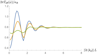
The conjecture is confirmed by results shown in fig. 13, where we represent for 3 different values of the upstream slope while holding fixed the downstream slope . Considering first the case with the lowest value of , and ignoring the small oscillations, we notice that there is a minimum length () at which the effective temperature becomes essentially -independent. This can be understood from the fact that, for , the length affects the typical gradient of the obstacle, as was discussed in Sec. II. When , a larger value of is required for the oscillations engendered by the upstream slope to be significantly reduced. This larger value of is such that , so that the reduction factor of the evanescent wave on reaching the upstream slope is around . Analyzing further the various curves, we verified that the differences in due to changes of (and thus ) are proportional to . Importantly we also verified that this remains true when considering frequencies other than . For all the frequencies we probed, the difference in becomes insignificant when .
To complete the analysis, in fig. 14 we plot how varies with for the 7 flows considered in Figures 6 and 7. Considering a fixed frequency, it is clear that there is a steady increase of with increasing . We also note that is fixed at zero for in subcritical flows, and only begins to increase once has reached a value at which . For a given value of , there is a frequency window in the high- part of the spectrum where this value is exceeded, and the lower limit of this window steadily decreases with . In fact, there exists some minimum value of above which this frequency window covers the entire spectrum. Therefore, given the result of fig. 13 that there exists a given value of above which no longer depends on , fig. 14 tells us that that this will be true of high frequencies before low frequencies, and that above a certain value of it will be true of the whole spectrum (except for the very small frequencies of Eq. (14), where the divergence of some scattering coefficients at the black hole horizon compensates the exponential decay).
In brief, what we learn here is that the emission spectrum of subcritical flows is more sensitive to the properties of the flow on its upstream side, since for a given frequency and length of the obstacle, is considerably smaller than in transcritical flows. This sensitivity of the scattering coefficients is further studied in App. B for obstacles similar to that used in the Vancouver experiment.
IV Conclusion
In this paper, we numerically studied the behavior of the 16 coefficients which enter in the -matrix governing the scattering of surface waves on a stationary flow above a localized obstacle. For simplicity, we assumed that the downstream flow was subcritical and asymptotically homogeneous, i.e., that it was not modulated by an extended zero-frequency wave (as is generally the case in practice, the undulation occurring on the downstream side).
In the first part of the work, we compared the 16 coefficients of a typical transcritical flow to those of a subcritical one. The main difference concerns the magnitude of the mode amplification: in transcritical flows some coefficients (relating unit norm modes) are substantially larger than 1, thereby revealing that the wave energy measured in the lab frame of some mode is significantly increased by the scattering. This large increase is made possible because of a correspondingly large emission of negative energy waves. In addition, when the flow is significantly transcritical, i.e., when (the maximal value of the Froude number) is larger than , the amplification factors closely follow the standard Hawking predictions. Namely, in a wide frequency regime, (the squared absolute value of the scattering coefficient mixing modes of opposite energy) follows a Planck law at a temperature in close agreement with , where is the analogue surface gravity evaluated where the local value of the Froude number crosses 1. By contrast, for subcritical flows no coefficient significantly surpasses 1, which means that there are no significant super-radiant effects.
We then focussed on the coefficients which describe the scattering of counter-propagating long wavelength modes, when gradually decreasing from a supercritical to a subcritical value. The effect on is the most dramatic. While in transcritical flows it behaves as in a wide domain of low , in subcritical flows it behaves as in a similarly large frequency domain. As a result, the maximal value of stays well below 1 for subcritical flows. Even in the transcritical case, however, there exists an ultra low frequency regime where is proportional to , because ultra low frequency modes are essentially transmitted across the obstacle. Interestingly, whenever scales as for , (the squared absolute value of the coefficient which relates incoming counterpropagating long wavelength modes to reflected short wavelength modes) follows . In fact, their ratio goes to 1 for .
In the second part, we analyzed the detailed properties of the same set of scattering coefficients in sub- and near-critical flows. We have shown the existence of high- and low-frequency behaviors separated by a transitionary regime around the critical frequency . Above this frequency the counterpropagating incoming long wavelength modes are essentially reflected, while below it they are essentially transmitted. As expected, the width of the frequency domain characterizing the transition decreases when increasing the length of the obstacle (at least for sufficiently narrow obstacles). We have also shown that this width tends to increase with increasing , and that it is largely independent of the slopes of the obstacle. In the low-frequency domain, we observed that for both in sub- and transcritical flows. We then showed that radically diminishes with increasing , see Fig. 10. In transcritical flows, this can be understood from the fact that , through its relationship to of Eq. (14), scales as the square of the damping factor of Eq. (21) associated with the evanescent mode, see also Fig. 14.
In the high-frequency regime of subcritical flows, the incoming long wavelength modes are essentially reflected, as is the case for transcritical flows. We could thus expect that the high-frequency scattering coefficients in trans- and subcritical flows behave in the same manner. However, our numerical observations indicate that this is only partially true. In particular, the scattering coefficients in subcritical flows are seen to be more sensitive to the upstream properties of the flow because there is a larger transmission across the obstacle. This larger sensitivity can be easily understood, and rather well characterized, by evaluating the residual amplitude of the evanescent wave on the upstream side of the obstacle. In addition, we have shown that the effective temperature characterizing the emitted flux significantly depends on the frequency at which it is measured. This means that the emitted flux in general does not follow the Planck law.
In Appendix A, as a function of the upstream and downstream slopes, we showed the behavior of the effective temperature evaluated in the low, the intermediate and the high frequency regimes. The existence of three different patterns demonstrates that the spectral properties radically differ in each regime. One should thus study each regime separately. In Appendix B we further studied the respective roles of the upstream and downstream slopes for asymmetrical obstacles which are similar to that used in Refs. Weinfurtner et al. (2011); Euvé et al. (2015a). For such narrow obstacles, i.e., obstacles such that the ratio of their effective length to the asymptotic water depth , our analysis reveals that the upstream slope, which is about 4 times larger than the dowstream slope, plays a dominant role in determining the scattering coefficients. Therefore, in future experiments, if one wishes to test the scattering on the downstream slope, it would be necessary to use either longer obstacles, or obstacles with a lower upstream slope.
Acknowledgments
SR would like to thank the University of Poitiers, and in particular Germain Rousseaux and Léo-Paul Euvé, for their welcome and hospitality while this work was being completed. This work was supported by the French National Research Agency by the Grants No. ANR-11-IDEX-0003-02 and ANR-15-CE30-0017-04 associated respectively with the project QEAGE (Quantum Effects in Analogue Gravity Experiments) and HARALAB. We also received support from a FQXi grant of the Silicon Valley Community Foundation.
Appendix A The 3 different behaviors of the spectrum
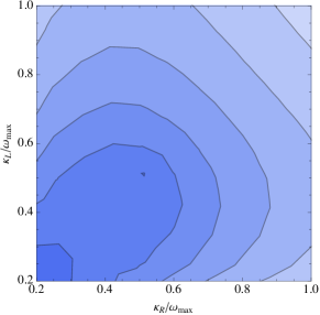
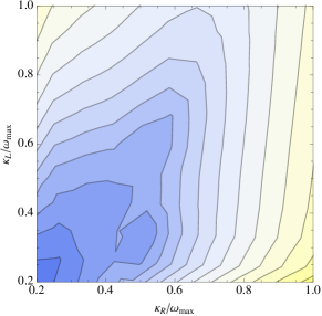
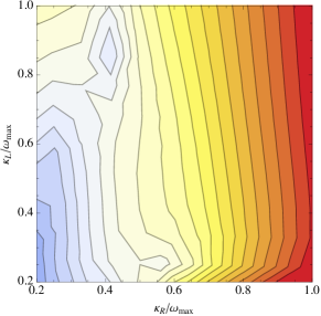
As a direct illustration of the existence of three different regimes, we show in Figure 15 contour plots of the effective temperature of Eq. (18) in the -plane (all quantities being adimensionalized by ), for frequencies , and . We clearly see that the shape of the contours radically differs for each plot. In particular, for the contours are symmetric about the diagonal , indicating that in the low-frequency regime the effective temperature is insensitive to the directionality of the flow; on the other hand, for the contours are more parallel to the -axis, indicating that the flow properties on the downstream side are more relevant in this regime. Much of the residual dependence on is due to our use of a narrow obstacle (we have used ); increasing , the contours for are more vertically aligned. We notice that the contours for are somehow in between the two we have just described. What we learn here is that it is inappropriate to look for a (global) description of the scattering that would be valid in the three regimes. This is why we study separately each regime in the main text.
Appendix B Effects of slope and asymmetry
When considering asymmetrical obstacles, there arises the interesting question of the respective roles of the upstream and downstream slopes in determining the scattering coefficients. To address this issue, we consider an obstacle described by Eq. (8) with properties similar to the one used in the Vancouver experiment. In particular, we take the upstream slope to be much larger than the downstream slope . The length parameter , corresponding to an effective length , is relatively short (compare with Figs. 8 and 9), a crucial property in that it allows the upstream slope to affect the scattering via tunnelling effects. The maximum and asymptotic Froude numbers are and , respectively.
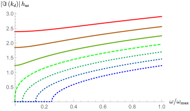
To illustrate the role of the asymmetry, we first compare the scattering on this flow to that on the reversed flow, i.e., the flow obtained by sending while keeping the orientation of the flow (from left to right) unchanged. Two important lessons can be drawn from fig. 16. For frequencies larger than , the temperatures and agree for any one flow, indicating that the unitarity condition (12) in the high-frequency domain is . However, there is a significant difference between the two orientations of the flow, as can be seen by comparing the red and blue curves. On the other hand, for frequencies smaller than , the situation is reversed: and become independent of the orientation of the flow, but are now in disagreement with each other. As already noted, vanishes for , while goes to a constant in this limit.
To further investigate the respective roles of and , we vary these quantities separately around the values given above. The results are shown in Figure 17 in terms of the two temperatures and of Eqs. (18) and (19), respectively. For either effective temperature, and irrespective of the orientation of the flow, one notices that the changes induced by varying the highest slope by , shown in the lower plots, are much more significant than those resulting from a variation of the lowest slope by the same relative amount, shown in the upper plots. Hence, for subcritical flows that are sufficiently short and asymmetrical, the scattering properties are mostly determined by the steepest slope, whether it is on the upstream or downstream side of the flow.
References
- Unruh (1981) W. G. Unruh, Phys. Rev. Lett. 46, 1351 (1981).
- Jacobson (1991) T. Jacobson, Phys. Rev. D44, 1731 (1991).
- Unruh (1995) W. G. Unruh, Phys. Rev. D51, 2827 (1995).
- Brout et al. (1995) R. Brout, S. Massar, R. Parentani, and P. Spindel, Phys. Rev. D52, 4559 (1995), arXiv:hep-th/9506121 [hep-th] .
- Corley and Jacobson (1996) S. Corley and T. Jacobson, Phys. Rev. D54, 1568 (1996), arXiv:hep-th/9601073 [hep-th] .
- Corley (1998) S. Corley, Phys. Rev. D57, 6280 (1998), arXiv:hep-th/9710075 [hep-th] .
- Unruh and Schutzhold (2005) W. G. Unruh and R. Schutzhold, Phys. Rev. D71, 024028 (2005), arXiv:gr-qc/0408009 [gr-qc] .
- Balbinot et al. (2005) R. Balbinot, A. Fabbri, S. Fagnocchi, and R. Parentani, Riv. Nuovo Cim. 28, 1 (2005), arXiv:gr-qc/0601079 [gr-qc] .
- Macher and Parentani (2009a) J. Macher and R. Parentani, Phys. Rev. D79, 124008 (2009a), arXiv:0903.2224 [hep-th] .
- Macher and Parentani (2009b) J. Macher and R. Parentani, Phys. Rev. A80, 043601 (2009b), arXiv:0905.3634 [cond-mat.quant-gas] .
- Finazzi and Parentani (2012) S. Finazzi and R. Parentani, Phys. Rev. D85, 124027 (2012), arXiv:1202.6015 [gr-qc] .
- Robertson (2012) S. J. Robertson, J. Phys. B45, 163001 (2012), arXiv:1508.02569 [gr-qc] .
- Coutant et al. (2012a) A. Coutant, R. Parentani, and S. Finazzi, Phys. Rev. D85, 024021 (2012a), arXiv:1108.1821 [hep-th] .
- Rousseaux et al. (2008) G. Rousseaux, C. Mathis, P. Maissa, T. G. Philbin, and U. Leonhardt, New J. Phys. 10, 053015 (2008), arXiv:0711.4767 [gr-qc] .
- Rousseaux et al. (2010) G. Rousseaux, P. Maissa, C. Mathis, P. Coullet, T. G. Philbin, and U. Leonhardt, New J. Phys. 12, 095018 (2010), arXiv:1004.5546 [gr-qc] .
- Weinfurtner et al. (2011) S. Weinfurtner, E. W. Tedford, M. C. J. Penrice, W. G. Unruh, and G. A. Lawrence, Phys. Rev. Lett. 106, 021302 (2011), arXiv:1008.1911 [gr-qc] .
- Euvé et al. (2015a) L.-P. Euvé, F. Michel, R. Parentani, and G. Rousseaux, Phys. Rev. D91, 024020 (2015a), arXiv:1409.3830 [gr-qc] .
- Euvé et al. (2015b) L. P. Euvé, F. Michel, R. Parentani, T. G. Philbin, and G. Rousseaux, (2015b), arXiv:1511.08145 [physics.flu-dyn] .
- Michel and Parentani (2014) F. Michel and R. Parentani, Phys. Rev. D90, 044033 (2014), arXiv:1404.7482 [gr-qc] .
- Michel and Parentani (2015) F. Michel and R. Parentani, (2015), arXiv:1508.02044 [gr-qc] .
- Coutant and Weinfurtner (2016) A. Coutant and S. Weinfurtner, (2016).
- Lawrence (1987) G. Lawrence, Journal of Hydraulic Engineering 113, 981 (1987), http://dx.doi.org/10.1061/(ASCE)0733-9429(1987)113:8(981) .
- Coutant and Parentani (2014) A. Coutant and R. Parentani, Phys.Fluids 26, 044106 (2014).
- Busch et al. (2014) X. Busch, F. Michel, and R. Parentani, Phys.Rev. D90, 105005 (2014), arXiv:1408.2442 [gr-qc] .
- Schutzhold and Unruh (2002) R. Schutzhold and W. G. Unruh, Phys. Rev. D66, 044019 (2002), arXiv:gr-qc/0205099 [gr-qc] .
- Unruh (2013) W. G. Unruh, Proceedings, 9th SIGRAV Graduate School in Contemporary Relativity and Gravitational Physics on Analogue Gravity Phenomenology, Lect. Notes Phys. 870, 63 (2013), arXiv:1205.6751 [gr-qc] .
- Bretherton and Garrett (1968) F. P. Bretherton and C. J. R. Garrett, Proc. Roy. Soc. A 302, 529 (1968), http://rspa.royalsocietypublishing.org/content/302/1471/529.full.pdf .
- Massar and Parentani (1998) S. Massar and R. Parentani, Nuclear Physics B 513, 375 (1998).
- Busch and Parentani (2014) X. Busch and R. Parentani, Phys. Rev. D 89, 105024 (2014).
- Coutant et al. (2012b) A. Coutant, S. Finazzi, S. Liberati, and R. Parentani, Phys. Rev. D85, 064020 (2012b), arXiv:1111.4356 [gr-qc] .
- Finazzi and Parentani (2011) S. Finazzi and R. Parentani, Journal of Physics: Conference Series 314, 012030 (2011).
- Leonhardt and Robertson (2012) U. Leonhardt and S. Robertson, New Journal of Physics 14, 053003 (2012).