Integrable $(2k)$-Dimensional Hitchin Equations

Abstract

This letter describes a completely-integrable system of Yang-Mills-Higgs equations which generalizes the Hitchin equations on a Riemann surface to arbitrary $k$-dimensional complex manifolds. The system arises as a dimensional reduction of a set of integrable Yang-Mills equations in $4k$ real dimensions. Our integrable system implies other generalizations such as the Simpson equations and the non-abelian Seiberg-Witten equations. Some simple solutions in the $k=2$ case are described.

MSC: 81T13, 53C26.

Keywords: gauge theory, Higgs, integrable system.

1 Introduction

This note concerns completely-integrable systems of Yang-Mills-Higgs equations, and in particular those which may be viewed as higher-dimensional generalizations of the two-dimensional Hitchin equations (the self-duality equations on a Riemann surface). Let us begin by briefly setting out the notation. We denote local coordinates on ${\mathbb{R}}^{n}$ by $x^{\mu}$ with $\mu=1,\ldots,n$. For simplicity we take the gauge group to be SU(2) throughout. A gauge potential $A_{\mu}$ takes values in the Lie algebra ${\mathfrak{s}u}(2)$, so each of $A_{1},\dots,A_{n}$ is an anti-hermitian $2\times 2$ matrix. The curvature (gauge field) is $F_{\mu\nu}=\partial_{\mu}A_{\nu}-\partial_{\nu}A_{\mu}+[A_{\mu},A_{\nu}]$. A Higgs field $\Phi$ takes values in the Lie algebra, or, if complex, in the complexified Lie algebra ${\mathfrak{s}l}(2,{\mathbb{C}})$. Its covariant derivative is $D_{\mu}=\partial_{\mu}\Phi+[A_{\mu},\Phi]$, and gauge transformations act by $\Phi\mapsto\Lambda^{-1}\Phi\Lambda$.

The prototype system is the simplest 2-dimensional reduction [14] of the 4-dimensional anti-self-dual Yang-Mills equations

$$F_{12}+F_{34}=0,\quad F_{13}+F_{42}=0,\quad F_{14}+F_{23}=0.$$ (1)

This reduction can be written as a conformally-invariant system on the complex plane ${\mathbb{C}}$, or more generally on a Riemann surface [12], and is effected as follows. If we take all the fields to depend only on the coordinates $(x^{1},x^{2})$, and we define a complex coordinate $z=x^{1}+ix^{2}$ and a complex Higgs field $\Phi=A_{3}+iA_{4}$, then (1) reduces to the Hitchin equations

$$D_{\bar{z}}\Phi=0,\quad F_{z\bar{z}}+\tfrac{1}{4}[\Phi,\Phi^{*}]=0.$$ (2)

Several higher-dimensional generalizations of (2) have been introduced and studied over the years. But most such generalizations lack a notable property of the original system (2), namely its complete integrability. The purpose of this note is to describe some features, and some solutions, of an integrable $(2k)$-dimensional generalization of (2).

Let us focus specifically on generalizations to $2k$ real (or $k$ complex) dimensions which involve $2k$ real (or $k$ complex) Higgs fields. Such systems may naturally be viewed as dimensional reductions of pure-gauge systems in $4k$ dimensions, satisfying linear relations on curvature such as (1). Of greatest interest are those that have the eigenvalue form [4]

$$F_{\mu\nu}=\tfrac{1}{2}T_{\mu\nu\alpha\beta}F_{\alpha\beta},$$ (3)

where $T_{\mu\nu\alpha\beta}$ is totally-skew, because the Bianchi identities then imply that the gauge field satisfies the second-order Yang-Mills equations.

Perhaps the best-known example is the ‘octonionic’ system of [4], which has $k=2$. This may be written

$$F_{12}+F_{34}+F_{56}+F_{78} =0,$$

$$F_{13}+F_{42}+F_{57}+F_{86} =0,$$

$$F_{14}+F_{23}+F_{76}+F_{85} =0,$$

$$F_{15}+F_{62}+F_{73}+F_{48} =0,$$

$$F_{16}+F_{25}+F_{38}+F_{47} =0,$$

$$F_{17}+F_{82}+F_{35}+F_{64} =0,$$

$$F_{18}+F_{27}+F_{63}+F_{54} =0.$$ (4)

Whereas the prototype (1) is essentially based on the quaternions, this system (4) is based on the octonions: the components of $T_{\mu\nu\alpha\beta}$ are constructed from the Cayley numbers. It is invariant under the group Spin(7), and its 7-dimensional reduction is invariant under $G_{2}$. We now reduce to four dimensions by requiring the fields to depend only on the variables $(x^{1},x^{2},x^{5},x^{6})$, defining two complex variables and two complex Higgs fields by

$$z^{1}=x^{1}+ix^{2},\quad z^{2}=x^{5}+ix^{6},\quad\Phi_{1}=A_{5}+iA_{6},\quad\Phi_{2}=A_{7}+iA_{8}.$$ (5)

Then the reduction of (4) is

$$F_{1\bar{1}}+F_{2\bar{2}}+\tfrac{1}{4}[\Phi_{1},\Phi_{1}^{*}]+\tfrac{1}{4}[\Phi_{2},\Phi_{2}^{*}] =0,$$

$$F_{12}-\tfrac{1}{4}[\Phi_{1},\Phi_{2}] =0,$$

$$D_{\bar{1}}\Phi_{1}-D_{2}\Phi_{2}^{*}=0,\,\,D_{\bar{2}}\Phi_{1}+D_{1}\Phi_{2}^{*} =0.$$ (6)

Here the subscript $1$ in $F_{1\bar{1}}$ and $D_{1}$ refers to $z^{1}$, whereas $\bar{1}$ refers to the complex conjugate variable $\bar{z}^{1}$. The equations (6) are more familiar in the ${\mathbb{R}}^{4}$ (real) form

$$\left(F-\tfrac{1}{2}[\Phi\wedge\Phi]\right)^{+}=0,\quad\left(D\Phi\right)^{-}=0,\quad D*\Phi=0,$$ (7)

where $\Phi=\Phi_{\mu}dx^{\mu}$ is a Lie-algebra-valued 1-form formed from the four real Higgs fields. The ‘plus’ superscript denotes the self-dual part of a 2-form, and the ‘minus’ superscript the anti-self-dual part. This system has appeared in several contexts over the years [6, 2, 13, 11, 8, 3], and has variously been referred to as the non-abelian Seiberg-Witten equations or the Kapustin-Witten equations. Known solutions include several obtained using a generalized ’t Hooft ansatz [7].

A different generalization of (2), defined on any Kähler manifold, is one attributed to Simpson [18]. In $k$ complex dimensions, with complex coordinates $z^{a}$, $a=1,\ldots,k$, it takes the form

$$F_{1\bar{1}}+\ldots+F_{k\bar{k}}+\tfrac{1}{4}[\Phi_{1},\Phi_{1}^{*}]+\ldots+\tfrac{1}{4}[\Phi_{k},\Phi_{k}^{*}] =0,$$

$$F_{ab}=0,\,\,[\Phi_{a},\Phi_{b}]=0,\,\,D_{\bar{a}}\Phi_{b}=0.$$ (8)

Note that for $k=1$, this system reduces to the prototype (2). For $k=2$, it clearly it implies (6). The converse is not true in general, but it is if one imposes appropriate global conditions: in particular for smooth fields on a compact Kähler surface, it has recently been shown that (8) and (6) are equivalent [19].

2 An integrable version

Another approach to generalizing the basic 4-dimensional system (1) is to look for higher-dimensional versions which are completely-integrable [20]. For simplicity, we begin with the case $k=2$. An integrable 8-dimensional Yang-Mills system is

$$F_{12}+F_{34} =F_{56}+F_{78}=0,$$

$$F_{13}+F_{42} =F_{57}+F_{86}=0,$$

$$F_{14}+F_{23} =F_{76}+F_{85}=0,$$

$$F_{15} =F_{26}=F_{37}=F_{48},$$

$$F_{16} =F_{52}=F_{83}=F_{47},$$

$$F_{17} =F_{28}=F_{53}=F_{64},$$

$$F_{18} =F_{72}=F_{36}=F_{54},$$ (9)

which clearly implies the octonionic equations (4). The system (9) has the symmetry group $\left[{\rm Sp(1)}\times{\rm Sp(2)}\right]/{\mathbb{Z}}_{2}\subset{\rm SO(8)}$, which corresponds to a quaternionic Kähler structure [17]. The ADHM construction of instantons [1] generalizes to this case [17, 5, 15]. Consider now the reduction to four dimensions, with the same complex variables (5) as before. Then (9) reduces to

$$D_{\bar{a}}\Phi_{b}=0,\,\,F_{a\bar{b}}+\tfrac{1}{4}[\Phi_{a},\Phi_{b}^{*}]=0,\,\,[\Phi_{a},\Phi_{b}]=0,\,\,F_{ab}=0,\,\,D_{[a}\Phi_{b]}=0,$$ (10)

where $a,b\in\{1,2\}$. This system is even more overdetermined than (8). So we have a string of implications, where (10) implies (8) implies (6) implies the four-dimensional Yang-Mills-Higgs equations (the reduction of pure Yang-Mills from eight dimensions).

Generalizing (10) to $k$ complex dimensions is straightforward: we simply allow the indices $a,b$ to range from $1$ to $k$. The system (10) has a very large symmetry group, since it involves only the holomorphic structure of the underlying complex manifold. This becomes clearer if we define

$$\Phi=\sum_{a}\Phi_{a}\,dz^{a}$$

as a $(1,0)$-form with values in the complexified Lie algebra: then (10) can be written

$$D\Phi=0,\,\,F^{1,1}+\tfrac{1}{4}[\Phi\wedge\Phi^{*}]=0,\,\,[\Phi\wedge\Phi]=0,\,\,F^{2,0}=0,$$ (11)

where $D$ now denotes the covariant exterior derivative. By contrast, the less-overdetermined systems (8) and (6) depend on an underlying geometric structure, and have less symmetry.

The system (10) is completely-integrable by virtue of being the consistency condition for a ‘Lax $(2k)$-tet’, namely

$$\eth_{a}=D_{a}+\tfrac{1}{2}\zeta\Phi_{a},\quad\eth_{\bar{a}}=D_{\bar{a}}+\tfrac{1}{2}\zeta^{-1}\Phi_{a}^{*},$$ (12)

where $\zeta$ is a complex parameter. The integrability conditions

$$[\eth_{a},\eth_{b}]=0=[\eth_{a},\eth_{\bar{b}}]$$

for all $\zeta$ are equivalent to the equations (10).

3 Some solutions

The aim now is to describe some solutions of (10); these will therefore also be solutions of the other systems (8), and (7) in the $k=2$ case. The equations (10) or (11) are defined on any $k$-dimensional complex manifold, and in general one may also allow singularities. For example, in the $k=1$ case on a compact Riemann surface of genus $g$, smooth solutions of (2) exist only when $g\geq 2$; on the 2-sphere and the 2-torus, solutions necessarily have singularities [12]. Note that the functions $G_{ab}=\mathop{\mathrm{tr}}\nolimits(\Phi_{a}\Phi_{b})$ are holomorphic, by virtue of the equations (11). In what follows, we look for solutions which are smooth on ${\mathbb{C}}^{2}$, and for which $G_{ab}$ is a polynomial in $z^{a}$. So they may also be viewed as being defined on the projective plane ${\mathbb{C}}{\mathbb{P}}^{2}$, with a singularity on the line at infinity.

To illustrate, let us first consider the abelian case, with the fields being diagonal, namely $\Phi_{a}=\phi_{a}\sigma_{3}$, where $\sigma_{3}={\rm diag}(1,\,-1)$. Then the equations (11) are easily solved. The gauge field vanishes, and therefore we may take the gauge potential to vanish as well. The remaining equations give $\Phi=d\theta$, where $\theta(z^{a})$ is an arbitrary polynomial on ${\mathbb{C}}^{2}$. This is the general abelian solution.

For the non-abelian SU(2) case, we adopt a simplifying ansatz which is familiar from the lower-dimensional version [10]. Namely let us assume that the gauge potential is diagonal: in other words, $A_{\bar{a}}=h_{\bar{a}}\sigma_{3}$. (It should be emphasized that there are solutions for which this assumption does not hold.) Then the general local solution is determined by a holomorphic function $\theta(z^{a})$, plus a solution $u=u(\theta,\bar{\theta})$ of the elliptic sinh-Gordon equation

$$\partial_{\theta}\partial_{\bar{\theta}}\log|u|=\tfrac{1}{4}\left(|u|^{2}-|u|^{-2}\right).$$ (13)

In terms of these, the Higgs fields are given by

$$\Phi_{a}=(\partial_{a}\theta)\left(\begin{matrix}0&u\\ u^{-1}&0\end{matrix}\right),$$

and the functions determining the gauge potential are

$$h_{\bar{a}}=-\tfrac{1}{2}\partial_{\bar{a}}\log(u).$$

Note that one solution of (13) is $u=1$, but this is effectively the abelian case of the previous paragraph. In order to get genuine non-abelian fields, we choose $\theta(z^{a})$ to have branch singularities, and then to get smooth fields one needs $u\neq 1$. The simplest such fields are embeddings of solutions of (2) on ${\mathbb{C}}$ into ${\mathbb{C}}^{2}$, depending on $z^{a}$ only via a fixed linear combination $z=\alpha z^{1}+\beta z^{2}$. For example, $\theta(z)=z^{3/2}$ gives an embedding of the ‘one-lump’ solution on ${\mathbb{C}}$ [21]. Some simple solutions that are not of this embedded type are as follows.

Let $P(z^{a})$ be a polynomial of degree at least two, and take $\theta=\tfrac{2}{3}P^{3/2}$. This gives Higgs fields of the form

$$\Phi_{a}=(\partial_{a}P)\left(\begin{matrix}0&P{\mathrm{e}}^{\psi/2}\\ {\mathrm{e}}^{-\psi/2}&0\end{matrix}\right),$$ (14)

where $\psi(P,\bar{P})$ satisfies

$$\partial_{P}\partial_{\bar{P}}\psi=\tfrac{1}{2}\left(|P|^{2}{\mathrm{e}}^{\psi}-{\mathrm{e}}^{-\psi}\right).$$ (15)

We now need a smooth solution of (15) satisfying the boundary condition $\psi\sim-\log|P|$ as $|P|\to\infty$. There exists a unique such solution, which is essentially a Painlevé-III function [9, 21]. In fact, if we define $h(t)=t^{-1/3}{\mathrm{e}}^{-\psi/2}$, where $t=|P|^{3/2}$, then (15) becomes an equation of Painlevé-III type, namely

$$h^{\prime\prime}-\frac{(h^{\prime})^{2}}{h}+\frac{h^{\prime}}{t}+\frac{4}{9h}-\frac{4h^{3}}{9}=0.$$ (16)

This has a unique solution with the required asymptotics.

The upshot is that any polynomial $P(z^{a})$ gives a solution of (11) which is smooth on ${\mathbb{C}}^{2}$ and has

$$G_{ab}=\mathop{\mathrm{tr}}\nolimits\left(\Phi_{a}\Phi_{b}\right)=2P(\partial_{a}P)(\partial_{b}P).$$

It appears (see for example the figure below) that the gauge field $F_{\mu\nu}$ is concentrated around the zero-set of $P$. In the general $k$-complex-dimensional case, one expects the gauge field to be concentrated around a submanifold of complex codimension 1, and for the field to be approximately abelian elsewhere.

The simplest case has $P$ quadratic, so that $P(z^{a})=0$ is a conic.

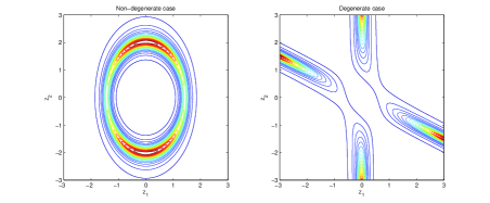
Figure 1: Contour plots of the gauge field $|F(z^{a})|$ for $z^{a}\in{\mathbb{R}}^{2}$, with $P(z^{a})=2(z^{1})^{2}+(z^{2})^{2}-4$ and $P(z^{a})=z^{1}(z^{1}+2z^{2})$ respectively.

Figure 1 is a plot of the norm $|F|$ of the gauge field, on the real slice $(z^{1},z^{2})\in{\mathbb{R}}^{2}$, for the solutions corresponding to the choices $P(z^{a})=2(z^{1})^{2}+(z^{2})^{2}-4$ (on the left), and $P(z^{a})=z^{1}(z^{1}+2z^{2})$ (on the right). Here $|F|$ is computed using the metric $ds^{2}=dz^{1}\,d\bar{z}^{1}+dz^{2}\,d\bar{z}^{2}$ on ${\mathbb{C}}^{2}$, which leads to the formula

$$|F|=\left|{\mathrm{e}}^{-\psi}-|P|^{2}{\mathrm{e}}^{\psi}\right|\left(|\partial_{1}P|^{2}+|\partial_{2}P|^{2}\right).$$ (17)

The figures were generated by solving (16) numerically to get $\psi$, and then using this formula (17). Clearly $|F|$ is concentrated around the conic $P(z^{a})=0$. The right-hand case corresponds to a degenerate conic, and is the reduced version of what was called ‘instantons at angles’ [16] for solutions of (9).

4 Remarks

There are some compact complex manifolds $X$ on which smooth solutions of (11) exist. As a trivial example, one could take $X$ to be a product $S\times X^{\prime}$, where $S$ is a Riemann surface of genus at least two, and $X^{\prime}$ is any other manifold: then a solution of (2) on $S$ is also a solution of (11) on $S\times X^{\prime}$. The moduli space of solutions on any compact manifold, if it is non-empty, has a natural $L^{2}$ metric, which on general grounds one expects to be hyperkähler. Even more generally, one could allow singularities of a specified type, or equivalently for the ambient space to be non-compact. In this latter case, some of the parameters in the solution space may have $L^{2}$ variation, giving rise to a moduli space with a well-defined metric. Analysing the possible moduli space geometries which arise in this way would be worthwhile, although a considerable task.

In this note, we have focused on a particular type of reduction of the integrable system (9), and of its $(4k)$-dimensional generalization. There are several other dimensional reductions of the octonionic system (4) which are of interest: see, for example, reference [3]. In each case, the appropriate reduction of (9) gives an integrable sub-system, and hence a source of solutions.

Acknowledgments. This work was prompted by a communication from Sergey Cherkis. The author acknowledges support from the UK Particle Science and Technology Facilities Council, through the Consolidated Grant ST/L000407/1.

References

- [1] Atiyah, M. F., Drinfeld, V. G., Hitchin, N. J. and Manin, Y. I.: Construction of instantons. Phys. Lett. A 65, 185–187 (1978).
- [2] Baulieu, L., Kanno, H. and Singer, I. M.: Special quantum field theories in eight and other dimensions. Commun. Math. Phys. 194, 149–175 (1998).
- [3] Cherkis, S. A.: Octonions, monopoles, and knots. Lett. MathṖhys. 105, 641–659 (2015).
- [4] Corrigan, E., Devchand, C., Fairlie, D. B. and Nuyts, J.: First-order equations for gauge fields in spaces of dimension greater than four. Nuclear Physics B 214, 452–464 (1983).
- [5] Corrigan, E., Goddard, P. and Kent, A.: Some comments on the ADHM construction in dimensions. Commun. Math. Phys. 100, 1–13 (1985).
- [6] Donaldson, S. K. and Thomas, R. P.: Gauge theory in higher dimensions. In: Huggett, S. A. et al (eds), The Geometric Universe, pp. 31–47. Oxford University Press, Oxford (1998).
- [7] Dunajski, M. and Hoegner, M.: SU(2) solutions to self-duality equations in eight dimensions. J. Geom. Phys. 62 1747–1759 (2012).
- [8] Gagliardo, M. and Uhlenbeck, K.: Geometric aspects of the Kapustin Witten equations. J. Fixed Point Theory Appl. 11, 185–198 (2012).
- [9] Gaiotto, D., Moore, G. W. and Neitzke, A.: Wall-crossing, Hitchin systems, and the WKB approximation. Adv. Math. 234, 239–403 (2013).
- [10] Harland, D. and Ward, R. S.: Dynamics of periodic monopoles. Physics Letters B 675, 262–266 (2009).
- [11] Haydys, A.: Gauge theory, calibrated geometry and harmonic spinors. J. London Math. Soc. 86, 482–498 (2012).
- [12] Hitchin, N. J.: The self-duality equations on a Riemann surface. Proc. Lond. Math. Soc. 55, 59–126 (1987).
- [13] Kapustin, A. and Witten, E.: Electromagnetic duality and the geometric Langlands program. Commun. Number Theory Phys. 1, 1–236 (2007).
- [14] Lohe, M. A.: Two- and three-dimensional instantons. Phys. Lett. B 70, 325–328 (1977).
- [15] Mamone Capria, M. and Salamon, S. M.: Yang-Mills fields on quaternionic spaces. Nonlinearity 1, 517–530 (1988).
- [16] Papadopoulos, G. and Teschendorff, A.: Instantons at angles. Physics Letters B 419, 115–122 (1998).
- [17] Salamon, S. M.: Quaternionic structures and twistor spaces. In: Willmore, T. J. and Hitchin, N. (eds), Global Riemannian Geometry, pp. 65–74. Ellis Horwood, Chichester (1984).
- [18] Simpson, C. T.: Constructing variations of Hodge structure using Yang-Mills theory and applications to uniformization. J. Amer. Math. Soc. 1, 867–918 (1988).
- [19] Tanaka, Y.: On the singular sets of solutions to the Kapustin-Witten equations on compact Kähler surfaces. (2015, ArXiv e-prints). arXiv:1510.07739
- [20] Ward, R. S.: Completely-solvable gauge-field equations in dimension greater than four. Nuclear Physics B 236, 381–396 (1984).
- [21] Ward, R. S.: Geometry of solutions of Hitchin equations on . Nonlinearity 29, 756–765 (2016).