The mean width of the oloid and
integral geometric applications of it

Abstract

The oloid is the convex hull of two circles with equal radius in perpendicular planes so that the center of each circle lies on the other circle. We calculate the mean width of the oloid in two ways, first via the integral of mean curvature, and then directly. Using this result, the surface area and the volume of the parallel body are obtained. Furthermore, we derive the expectations of the mean width, the surface area and the volume of the intersections of a fixed oloid and a moving ball, as well as of a fixed and a moving oloid.
2010 Mathematics Subject Classification: 53A05, 52A15, 52A22, 60D05
Keywords: Oloid, convex hull, integral of mean curvature, mean width, Steiner formula, parallel body, intrinsic volumes, principal kinematic formula

1 Introduction

The oloid $\varOmega_{r}$ is the convex hull of two circles $k_{A}$, $k_{B}$ with equal radius $r$ in perpendicular planes so that the center of each circle lies on the other circle (see Figures 2 and 2). Dirnböck & Stachel [4, p. 117] calculated the surface area and the volume of the oloid (see also [14], [15], and Equations (2), (6), (2) and (8) of the present paper). The surface $\partial\varOmega_{r}$ is part of a developable surface [4], [2], [14], [15].

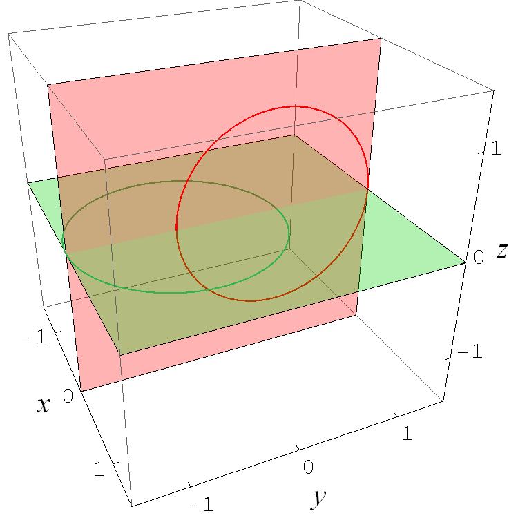
Figure 1: The circles $k_{A}$ and $k_{B}$ with $r=1$

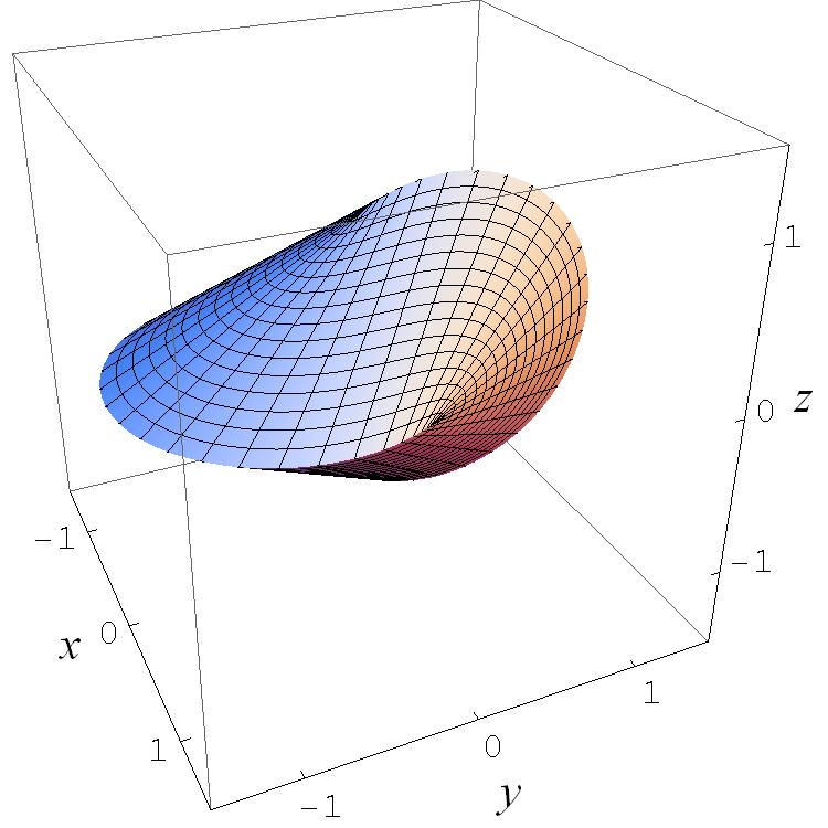
Figure 2: The oloid $\varOmega_{1}$

Finch [5] calculated surface areas, volumes and mean widths of the convex hulls of three different configurations of two orthogonal disks with equal radius. The mean width $\bar{b}$ of every convex hull is determined twice: 1) using the integral $M$ of the mean curvature and the relation $\bar{b}=M/(2\pi)$, 2) calculating $\bar{b}$ directly.
     According to [4, pp. 105-106], the circles with $r=1$ can be defined by

$$k_{A}:={} \left\{(x,y,z)\in\mathbb{R}^{3}\colon x^{2}+(y+1/2)^{2}=1\wedge z=0\right\},$$ (1)

$$k_{B}:={} \left\{(x,y,z)\in\mathbb{R}^{3}\colon(y-1/2)^{2}+z^{2}=1\wedge x=0\right\}$$

(see Fig. 1). A parametrization of the surface $\partial\varOmega_{1}$ [2, p. 165, Eq. (2)] is

$$(x,y,z)^{\textnormal{T}}=\vec{\omega}(m,t)=(\omega_{1}(m,t),\omega_{2}(m,t),\pm\omega_{3}(m,t))^{\textnormal{T}}\,,\quad 0\leq m\leq 1\,,\quad-\frac{2\pi}{3}\leq t\leq\frac{2\pi}{3}\,,$$ (2)

with

$$\left.\begin{aligned} \omega_{1}(m,t)={}&(1-m)\sin t\,,\\[2.84544pt] \omega_{2}(m,t)={}&\frac{2(m-1)\cos^{2}t+(2m-3)\cos t+2m-1}{2(1+\cos t)}\,,\\ \omega_{3}(m,t)={}&\frac{m\sqrt{1+2\cos t}}{1+\cos t}\,.\end{aligned}\;\;\right\}$$ (3)

To the authors knowledge, the mean width of the oloid is not aready known. In Section 3 we calculate the mean width of $\varOmega_{r}$ using the integral of mean curvature, and in Section 4 we calculate it directly. With the help of this result we derive the volume, the surface area and the mean width of the parallel body of $\varOmega_{r}$ in Section 5. Using the principal kinematic formula of integral geometry, the expectations of the mean width, the surface area and the volume of the intersections of a fixed oloid and a moving ball, as well as of a fixed and a moving oloid are calculated in Section 6.

2 Preliminaries

In the following, we work in the real vector space $\mathbb{R}^{3}$ with its standard scalar product $\big{\langle}\vec{a},\vec{b}\,\big{\rangle}=\vec{a}\,\cdot\,\vec{b}$ and its vector product $\vec{a}\times\vec{b}$ for two vectors $\vec{a}=(a_{1},a_{2},a_{3})^{\textnormal{T}}$, $\vec{b}=(b_{1},b_{2},b_{3})^{\textnormal{T}}$. We denote the partial derivatives

$$\frac{\partial\vec{\omega}}{\partial m}\,,\quad\frac{\partial\vec{\omega}}{\partial t}$$

of $\vec{\omega}=\vec{\omega}(m,t)$ (see (2)) by $\vec{\omega}_{m}$, $\vec{\omega}_{t}$, and so on.
     Using (3), for the coefficients $g_{11}=E$, $g_{12}=F=g_{21}$, $g_{22}=G$ of the first fundamental form (see e. g. [6, pp. 87-88], translation: p. 68) we find

$$\left.\begin{aligned} g_{11}={}&\langle\vec{\omega}_{m},\vec{\omega}_{m}\rangle=3\,,\qquad g_{12}=\langle\vec{\omega}_{m},\vec{\omega}_{t}\rangle=\tan(t/2)\,,\\[2.84544pt] g_{22}={}&\langle\vec{\omega}_{t},\vec{\omega}_{t}\rangle=\frac{2(3m^{2}-4m+1)\cos^{2}t-(4m-3)\cos t+1}{(1+\cos t)(1+2\cos t)}\,,\\[2.84544pt] g={}&\det(g_{jk})=\left|\begin{array}[]{ll}g_{11}&g_{12}\\ g_{21}&g_{22}\end{array}\right|=g_{11}\,g_{22}-g_{12}^{2}=\frac{2[(3m-2)\cos t-1]^{2}}{(1+\cos t)(1+2\cos t)}\,.\end{aligned}\;\;\right\}$$ (4)

Now, we able to calculate the surface area of the oloid $\varOmega_{1}$:

$$S(\varOmega_{1})={} \int_{\partial\varOmega_{1}}\mathrm{d}S=\int_{\partial\varOmega_{1}}\mathrm{d}S(m,t)=2\int_{t=-2\pi/3}^{2\pi/3}\,\int_{m=0}^{1}\sqrt{g(m,t)}\>\mathrm{d}m\,\mathrm{d}t$$

$$={} 4\int_{t=0}^{2\pi/3}\int_{m=0}^{1}\sqrt{g(m,t)}\>\mathrm{d}m\,\mathrm{d}t=4\int_{t=0}^{2\pi/3}\int_{m=0}^{1}\frac{\sqrt{2}\left[(2-3m)\cos t+1\right]}{\sqrt{(1+\cos t)(1+2\cos t)}}\,\mathrm{d}m\,\mathrm{d}t$$

$$={} 2\,\sqrt{2}\int_{0}^{2\pi/3}\frac{2+\cos t}{\sqrt{(1+\cos t)(1+2\cos t)}}\,\mathrm{d}t\,.$$ (5)

Mathematica evaluates this integral to

$$S(\varOmega_{1})=2\,\sqrt{2}\cdot\sqrt{2}\,\pi=4\pi\,.$$ (6)

Now, we calculate the volume of $\varOmega_{1}$, and start with

$$V(\varOmega_{1})={} 2\iint z\,\mathrm{d}x\,\mathrm{d}y=2\int_{t=-2\pi/3}^{2\pi/3}\,\int_{m=0}^{1}\omega_{3}(m,t)\left|\frac{\partial(\omega_{1}(m,t),\,\omega_{2}(m,t))}{\partial(m,t)}\right|\mathrm{d}m\,\mathrm{d}t$$

$$={} 4\int_{t=0}^{2\pi/3}\,\int_{m=0}^{1}\omega_{3}(m,t)\left|\frac{\partial(\omega_{1}(m,t),\,\omega_{2}(m,t))}{\partial(m,t)}\right|\mathrm{d}m\,\mathrm{d}t\,.$$

From (3) it follows that

$$\frac{\partial(\omega_{1}(m,t),\,\omega_{2}(m,t)}{\partial(m,t)}=\left|\begin{array}[]{ll}\displaystyle{\frac{\partial\omega_{1}(m,t)}{\partial m}}&\displaystyle{\frac{\partial\omega_{1}(m,t)}{\partial t}}\\[8.5359pt] \displaystyle{\frac{\partial\omega_{2}(m,t)}{\partial m}}&\displaystyle{\frac{\partial\omega_{2}(m,t)}{\partial t}}\end{array}\right|=-\frac{1+(2-3m)\cos t}{1+\cos t}\,.$$

So we have

$$V(\varOmega_{1})={} 4\int_{t=0}^{2\pi/3}\int_{m=0}^{1}\frac{m\,\sqrt{1+2\cos t}}{1+\cos t}\,\frac{1+(2-3m)\cos t}{1+\cos t}\,\mathrm{d}m\,\mathrm{d}t$$

$$={} 2\int_{0}^{2\pi/3}\frac{\sqrt{1+2\cos t}}{(1+\cos t)^{2}}\,\mathrm{d}t\,.$$ (7)

Mathematica finds

$$V(\varOmega_{1})=\frac{2}{3}\left[K\big{(}\sqrt{3}\big{/}2\big{)}+2E\big{(}\sqrt{3}\big{/}2\big{)}\right],$$ (8)

where

$$K(k)=F(\pi/2,k)=\int_{0}^{\pi/2}\frac{\mathrm{d}x}{\sqrt{1-k^{2}\sin^{2}x}}\,,$$ (9)

is the complete elliptic integral of the first kind, and

$$E(k)=E(\pi/2,k)=\int_{0}^{\pi/2}\sqrt{1-k^{2}\sin^{2}x}\,\mathrm{d}x$$ (10)

is the complete elliptic integral of the second kind. A numerical integration integration of (2) and evaluation of (8) with Mathematica yields the decimal expansion

$$V(\varOmega_{1})\approx 3.05241846842437485669720053193$$

(see also [1]).

3 The integral of mean curvature

The surface $\partial\varOmega_{1}$ of the oloid $\varOmega_{1}$ is piecewise continuously differentiable. We denote by $H$ the mean curvature in one point of $\partial\varOmega_{1}$. The circles $k_{A}$ and $k_{B}$ (see (1)) produce two edges $\varepsilon_{1}$ and $\varepsilon_{2}$, respectively, that are smooth curves. Let $\alpha=\alpha(t)$ denote the angle between the two unit normal vectors in every point of $\varepsilon_{1}$. Applying the general formula for the integral $M$ of the mean curvature (see [12, pp. 76-77, Eqs. (3.5), (3.7)]; cp. the formula for the mean width in [5, p. 3]) to $\varOmega_{1}$ gives

$$M(\varOmega_{1})=\int_{\partial\varOmega_{1}}H\,\mathrm{d}S+\frac{1}{2}\,\sum_{j=1}^{2}\int_{\varepsilon_{j}}\alpha\,\mathrm{d}s=\int_{\partial\varOmega_{1}}H(m,t)\>\mathrm{d}S(m,t)+\int_{\varepsilon_{1}}\alpha(t)\,\mathrm{d}t$$ (11)

For the unit normal vector one finds

$$\vec{n}=(n_{1},n_{2},n_{3})^{\textnormal{T}}=\frac{\vec{\omega}_{m}\times\vec{\omega}_{t}}{\lvert\vec{\omega}_{m}\times\vec{\omega}_{t}\rvert}=\left(\sin(t/2)\,,\>-\frac{\cos t}{2\cos(t/2)}\,,\>\frac{\sqrt{1+2\cos t}}{2\cos(t/2)}\,\right)^{\textnormal{\!\!T}}.$$ (12)

Since $\partial\varOmega_{1}$ is part of a developable surface and the line segments $t=\textnormal{const}$, $0\leq m\leq 1$ are part of the generators of $\partial\varOmega_{1}$ (see [4], [2]), it is not surprising that $\vec{n}$ does not depend on $m$. The mean curvature in a point of a surface is defined by

$$H=\frac{1}{2}\,(\kappa_{1}+\kappa_{2})=\frac{1}{2g}\,(g_{11}b_{22}-2g_{12}b_{12}+g_{22}b_{11})\,,$$

where $\kappa_{1}$, $\kappa_{2}$ are the principal curvatures, $b_{ik}$ are the coefficients of the second fundamental form (see e. g. [6, p. 99], translation: p. 79), and $g_{ik}$, $g$ are given by (4). In our case we have

$$H(m,t)\,\mathrm{d}S(m,t)=H(m,t)\,\sqrt{g(m,t)}\,\mathrm{d}m\,\mathrm{d}t=\frac{1}{2\,\sqrt{g}}\,(g_{11}b_{22}-2g_{12}b_{12}+g_{22}b_{11})\,\mathrm{d}m\,\mathrm{d}t$$

and

$$b_{11}={} L=\langle\vec{\omega}_{mm},\vec{n}\rangle=0\,,\qquad b_{12}=M=\langle\vec{\omega}_{mt},\vec{n}\rangle=0\,,$$

$$b_{22}={} N=\langle\vec{\omega}_{tt},\vec{n}\rangle=\frac{(3m-2)\cos t-1}{\sqrt{2}\,(1+2\cos t)\,\sqrt{1+\cos t}}\,.$$

It follows that

$$H(m,t)\,\mathrm{d}S(m,t)={} \frac{g_{11}(m,t)b_{22}(m,t)}{2\,\sqrt{g(m,t)}}\>\mathrm{d}m\,\mathrm{d}t$$

$$={} \frac{3}{2}\cdot\frac{(3m-2)\cos t-1}{\sqrt{2}\,(1+2\cos t)\,\sqrt{1+\cos t}}\cdot\frac{\sqrt{1+\cos t}\,\sqrt{1+2\cos t}}{\sqrt{2}\,[(3m-2)\cos t-1]}\,\mathrm{d}m\,\mathrm{d}t$$

$$={} \frac{3}{4\,\sqrt{1+2\cos t}}\,\mathrm{d}m\,\mathrm{d}t$$

and

$$\int_{\partial\varOmega_{1}}H\,\mathrm{d}S={} 2\int_{m=0}^{1}\int_{t=-2\pi/3}^{2\pi/3}H(m,t)\,\mathrm{d}S(m,t)=\frac{3}{2}\int_{0}^{1}\mathrm{d}m\>\int_{-2\pi/3}^{2\pi/3}\frac{1}{\sqrt{1+2\cos t}}\,\mathrm{d}t$$

$$={} \frac{3}{2}\int_{-2\pi/3}^{2\pi/3}\frac{1}{\sqrt{1+2\cos t}}\,\mathrm{d}t=3\int_{0}^{2\pi/3}\frac{1}{\sqrt{1+2\cos t}}\,\mathrm{d}t\,.$$

Mathematica finds

$$\int_{0}^{2\pi/3}\frac{\mathrm{d}t}{\sqrt{1+2\cos t}}\,\mathrm{d}t=K\big{(}\sqrt{3}\big{/}2\big{)}\,,$$ (13)

where $K$ is the complete elliptic integral of the first kind (9), hence

$$\int_{\partial\varOmega_{1}}H\,\mathrm{d}S=3K\big{(}\sqrt{3}\big{/}2\big{)}\,.$$ (14)

A handmade proof for the relation in (13) may be found in Section 7.
     Now we calculate the integral of mean curvature for the edges $\varepsilon_{1}$, $\varepsilon_{2}$ (see (11)). Therefore, we consider $\varepsilon_{1}$. The first unit normal vector $\vec{n}=\vec{n}(t)$ in a point $t\in[-2\pi/3,2\pi/3]$, $m=0$ is given by (12), the second is $\vec{n}^{*}=\vec{n}^{*}(t)=(n_{1},n_{2},-n_{3})^{\textnormal{T}}$. So one gets

$$\alpha(t)=\arccos\langle\vec{n}(t),\vec{n}^{*}(t)\rangle=\arccos\left(\!-\frac{\cos t}{1+\cos t}\right),$$

hence

$$\int_{\varepsilon_{1}}\alpha\,\mathrm{d}t=\int_{-2\pi/3}^{2\pi/3}\alpha(t)\,\mathrm{d}t=2\int_{0}^{2\pi/3}\alpha(t)\,\mathrm{d}t=2\int_{0}^{2\pi/3}\arccos\left(\!-\frac{\cos t}{1+\cos t}\right)\,\mathrm{d}t\,.$$

We observe that the inverse function of the integrand is equal to the integrand, and hence the graph of the integrand symmetrical with respect to the line $f(t)=t$. As solution of

$$f(t)=t=\arccos\left(\!-\frac{\cos t}{1+\cos t}\right)$$

we find $t=\pi/2$, hence

$$\int_{\varepsilon_{1}}\alpha\,\mathrm{d}t={} 4\int_{0}^{\pi/2}\left[\arccos\left(\!-\frac{\cos t}{1+\cos t}\right)-t\right]\mathrm{d}t=4\int_{0}^{\pi/2}\arccos\left(\!-\frac{\cos t}{1+\cos t}\right)\mathrm{d}t-4\int_{0}^{\pi/2}t\,\mathrm{d}t$$

$$={} 4\int_{0}^{\pi/2}\arccos\left(\!-\frac{\cos t}{1+\cos t}\right)\mathrm{d}t-\frac{\pi^{2}}{2}=4\int_{0}^{\pi/2}\left[\pi-\arccos\frac{\cos t}{1+\cos t}\right]\mathrm{d}t-\frac{\pi^{2}}{2}$$

$$={} 4\pi\int_{0}^{\pi/2}\mathrm{d}t-4\int_{0}^{\pi/2}\arccos\frac{\cos t}{1+\cos t}\,\mathrm{d}t-\frac{\pi^{2}}{2}$$

$$={} \frac{3\pi^{2}}{2}-4\int_{0}^{\pi/2}\arccos\frac{\cos t}{1+\cos t}\,\mathrm{d}t\,.$$ (15)

Mathematica and we, too, are not able to solve the last integral. It looks similar to Coxeter’s integral in [7, pp. 194-201]. The NIntegrate-function of Mathematica provides

$$I:=\int_{0}^{\pi/2}\arccos\frac{\cos t}{1+\cos t}\,\mathrm{d}t\approx 1.87738105428247449505835371657\,,$$ (16)

hence

$$\int_{\varepsilon_{1}}\alpha\,\mathrm{d}t\approx 7.29488238450413994801832163353\,.$$

From (11), (14), (3), with (9) and (16), it follows that the integral $M$ of the mean curvature of $\varOmega_{r}$ is given by

$$M(\varOmega_{r})=\left(3K\big{(}\sqrt{3}\big{/}2\big{)}+\frac{3\pi^{2}}{2}-4I\right)r\approx 13.7644293270030696543343466299\,r\,.$$

For a convex body $K$, the mean width $\bar{b}$ is given by the relation $\bar{b}(K)=M(K)/2\pi$ (see [12, p. 78, Eq. (3.9)]). So we we have proved the following theorem.

Theorem 1.

The mean width of the oloid $\varOmega_{r}$ is

$$\bar{b}(\varOmega_{r})=\left(\frac{3}{2\pi}\,K\big{(}\sqrt{3}\big{/}2\big{)}+\frac{3\pi}{4}-\frac{2}{\pi}\,I\right)r\approx 2.19067696623158876633263049436\,r,$$

where $K$ is the complete elliptic integral of the first kind (9), and

$$I=\int_{0}^{\pi/2}\arccos\frac{\cos x}{1+\cos x}\,\mathrm{d}x\,.$$

4 Direct calculation of the mean width

Let

$$P=\{(x,y,z)\in\mathbb{R}^{3}\colon ax+by+cz=d\}$$

be a supporting plane of $\varOmega_{1}$ given in the Hesse normal form. So $\vec{N}=(a,b,c)^{\textnormal{T}}$ with $a,b,c\in\mathbb{R}$, $a^{2}+b^{2}+c^{2}=1$ is the normal unit vector of $P$ and $|d|$ is the distance of $P$ from the origin. $P$ intersects the plane $z=0$ in the line

$$L_{xy}=\{(x,y)\in\mathbb{R}^{2}\colon ax+by=d\}\,,$$

and the plane $x=0$ in the line

$$L_{yz}=\{(y,z)\in\mathbb{R}^{2}\colon by+cz=d\}\,.$$

The equation of $L_{xy}$ in Hesse normal form is

$$\frac{ax}{\sqrt{a^{2}+b^{2}}}+\frac{by}{\sqrt{a^{2}+b^{2}}}=\frac{d}{\sqrt{a^{2}+b^{2}}}\,,$$

therefore, the distance $d_{1}$ of $L_{xy}$ from the center $(0,-1/2,0)$ of $k_{A}$ is

$$d_{1}=\left|\frac{a}{\sqrt{a^{2}+b^{2}}}\cdot 0+\frac{b}{\sqrt{a^{2}+b^{2}}}\cdot\left(\!-\frac{1}{2}\right)-\frac{d}{\sqrt{a^{2}+b^{2}}}\right|=\frac{b/2+d}{\sqrt{a^{2}+b^{2}}}$$

(see e. g. [3, p. 172]). Since $L_{xy}$ is tangent to $k_{A}$, we have

$$\frac{b/2+d}{\sqrt{a^{2}+b^{2}}}=1\qquad\Longrightarrow\qquad d=\sqrt{a^{2}+b^{2}}-\frac{b}{2}\,.$$

Analogously one finds that the distance $d_{2}$ of $L_{yz}$ from the center $(0,1/2,0)$ of $k_{B}$ is

$$d_{2}=\frac{b/2-d}{\sqrt{a^{2}+b^{2}}}=1\,,$$

hence

$$d=\sqrt{a^{2}+b^{2}}+\frac{b}{2}\,.$$

It follows that the distance $p$ between the support plane $P$ and the origin is

$$p=\max\left\{\sqrt{a^{2}+b^{2}}-\frac{b}{2},\sqrt{a^{2}+b^{2}}+\frac{b}{2}\right\}.$$

Now we use spherical coordinates $0\leq\varphi\leq\pi/2$ and $0\leq\vartheta\leq\pi/2$ as coordinates of the unit normal vector $\vec{N}$:

$$a=\cos\varphi\sin\vartheta\,,\quad b=\sin\varphi\sin\vartheta\,,\quad c=\cos\vartheta\,.$$

So we have

$$\sqrt{a^{2}+b^{2}}-\frac{b}{2}={} \left(1-\frac{1}{2}\,\sin\varphi\right)\sin\vartheta\,,$$

$$\sqrt{a^{2}+b^{2}}+\frac{b}{2}={} \frac{1}{2}\,\sin\varphi\sin\vartheta+\sqrt{\sin^{2}\varphi\sin^{2}\vartheta+\cos^{2}\vartheta}\,,$$

and can write $p$ as

$$p(\varphi,\vartheta)=\max\left\{\left(1-\frac{1}{2}\sin\varphi\right)\sin\vartheta,\frac{1}{2}\sin\varphi\sin\vartheta+\sqrt{\sin^{2}\varphi\sin^{2}\vartheta+\cos^{2}\vartheta}\right\}.$$

Clearly, $p=p(\varphi,\vartheta)$ is the support function of $\varOmega_{1}$ in the direction $\varphi,\vartheta$. Hence the width $b$ of $\varOmega_{r}$ in this direction is given by

$$b(\varphi,\vartheta)=p(\varphi,\vartheta)+p(\pi+\varphi,\pi-\vartheta)\,.$$

In order to calculate the mean width $\bar{b}$ of $\varOmega_{1}$ we have to integrate over all directions, hence over the unit hemisphere. Let $\mathrm{d}S=\mathrm{d}S(\varphi,\vartheta)=\sin\vartheta\,\mathrm{d}\vartheta\,\mathrm{d}\varphi$ denote the surface element of the unit sphere, we have

$$\bar{b}(\varOmega_{1})={} \frac{\int_{0}^{\pi}\int_{0}^{\pi}b(\varphi,\vartheta)\,\mathrm{d}S(\varphi,\vartheta)}{\int_{0}^{\pi}\int_{0}^{\pi}\mathrm{d}S(\varphi,\vartheta)}=\frac{\int_{0}^{\pi}\int_{0}^{\pi}[p(\varphi,\vartheta)+p(\pi+\varphi,\pi-\vartheta)]\,\mathrm{d}S(\varphi,\vartheta)}{\int_{0}^{\pi}\int_{0}^{\pi}\mathrm{d}S(\varphi,\vartheta)}$$

$$={} \frac{\int_{0}^{\pi}\int_{0}^{\pi}p(\varphi,\vartheta)\,\mathrm{d}S(\varphi,\vartheta)+\int_{0}^{\pi}\int_{0}^{\pi}p(\pi+\varphi,\pi-\vartheta)\,\mathrm{d}S(\varphi,\vartheta)}{\int_{0}^{\pi}\int_{0}^{\pi}\mathrm{d}S(\varphi,\vartheta)}=\frac{2\int_{0}^{\pi}\int_{0}^{\pi}p(\varphi,\vartheta)\,\mathrm{d}S(\varphi,\vartheta)}{\int_{0}^{\pi}\int_{0}^{\pi}\mathrm{d}S(\varphi,\vartheta)}$$

(cp. [12, p. 78, Eq. (3.9)]), where the last equal sign follows from the fact that there are two congruent portions of $\varOmega_{1}$ in the half spaces $y\leq 0$ and $y\geq 0$. Due to the symmetry of $\varOmega_{1}$ with respect to the planes $z=0$ and $x=0$ we can restrict the spherical coordiates to the intervals $0\leq\vartheta\leq\pi/2$ and $0\leq\varphi\leq\pi/2$, respectively, hence

$$\bar{b}(\varOmega_{1})={} \frac{2\int_{0}^{\pi/2}\int_{0}^{\pi/2}p(\varphi,\vartheta)\,\mathrm{d}S(\varphi,\vartheta)}{\int_{0}^{\pi/2}\int_{0}^{\pi/2}\mathrm{d}S(\varphi,\vartheta)}=\frac{2\int_{0}^{\pi/2}\int_{0}^{\pi/2}p(\varphi,\vartheta)\sin\vartheta\,\mathrm{d}\vartheta\,\mathrm{d}\varphi}{\int_{0}^{\pi/2}\int_{0}^{\pi/2}\sin\vartheta\,\mathrm{d}\vartheta\,\mathrm{d}\varphi}$$

$$={} \frac{4}{\pi}\int_{0}^{\pi/2}\int_{0}^{\pi/2}p(\varphi,\vartheta)\sin\vartheta\,\mathrm{d}\vartheta\,\mathrm{d}\varphi$$

$$={} \frac{4}{\pi}\left[\int_{\varphi=0}^{\pi/6}\int_{\vartheta=0}^{\xi(\varphi)}\left(\frac{1}{2}\sin\varphi\sin\vartheta+\sqrt{\sin^{2}\varphi\sin^{2}\vartheta+\cos^{2}\vartheta}\right)\sin\vartheta\,\mathrm{d}\vartheta\,\mathrm{d}\varphi\right.$$

$$+\int_{\varphi=0}^{\pi/6}\>\int_{\vartheta=\xi(\varphi)}^{\pi/2}\left(1-\frac{1}{2}\,\sin\varphi\right)\sin^{2}\vartheta\,\mathrm{d}\vartheta\,\mathrm{d}\varphi$$ (17)

$$+\left.\int_{\varphi=\pi/6}^{\pi/2}\int_{\vartheta=0}^{\pi/2}\left(\frac{1}{2}\sin\varphi\sin\vartheta+\sqrt{\sin^{2}\varphi\sin^{2}\vartheta+\cos^{2}\vartheta}\right)\sin\vartheta\,\mathrm{d}\vartheta\,\mathrm{d}\varphi\right],$$

where

$$\xi(\varphi)=\arccos\frac{\sqrt{-1+2\sin\varphi}}{\sqrt{-2+2\sin\varphi}}$$

is the solution of the equation

$$\left(1-\frac{1}{2}\sin\varphi\right)\sin\vartheta=\frac{1}{2}\sin\varphi\sin\vartheta+\sqrt{\sin^{2}\varphi\sin^{2}\vartheta+\cos^{2}\vartheta}$$

for $\vartheta=\xi(\varphi)$. Numerical integration of (4) with Mathematica gives

$$\bar{b}(\varOmega_{1})\approx 2.19067696623\,.$$

5 The parallel body

For a convex body $K\subset\mathbb{R}^{n}$ and $\varrho>0$, the set (Minkowski sum)

$$K+B_{\varrho}^{n}=\{x\in\mathbb{R}^{n}\colon d(x,K)\leq\varrho\}$$

is the parallel body of $K$ at distance $\varrho$, where $B_{\varrho}^{n}$ is the $n$-ball of radius $\varrho$,

$$B_{\varrho}^{n}=\{x\in\mathbb{R}^{n}\colon\lVert x\rVert\leq\varrho\}\,,$$

and $d(x,K)$ is the distance between the point $x$ and $K$. The volume of the parallel body is given by the Steiner formula

$$V_{n}(K+B_{\varrho}^{n})=\sum_{j=0}^{n}\varrho^{n-j}\kappa_{n-j}V_{j}(K)\,,$$ (18)

where

$$\kappa_{k}=\frac{\pi^{k/2}}{\varGamma(1+k/2)}$$ (19)

is the volume of the $k$-dimensional unit ball $B_{1}^{k}$, and $V_{0},\ldots,V_{n-1}$ are the intrinsic volumes of $K$. [11, p. 2, pp. 12-13, p. 600]
     Using the relations in [10, p. 301], where $\chi$ denotes the Euler characteristic, the intrinsic volumes of $\varOmega_{r}$ are

$$\left.\begin{aligned} V_{0}(\varOmega_{r})={}&\chi=1\,,\quad V_{1}(\varOmega_{r})=2\bar{b}(\varOmega_{r})=\frac{M(\varOmega_{r})}{\pi}=\left[\frac{3}{\pi}\,K\big{(}\sqrt{3}\big{/}2\big{)}+\frac{3\pi}{2}-\frac{4}{\pi}\,I\right]r\,,\\[2.84544pt] V_{2}(\varOmega_{r})={}&\frac{1}{2}\,S(\varOmega_{r})=2\pi r^{2}\,,\quad V_{3}(\varOmega_{r})=V(\varOmega_{r})=\frac{2}{3}\left[2E\big{(}\sqrt{3}\big{/}2\big{)}+K\big{(}\sqrt{3}\big{/}2\big{)}\right]r^{3}\end{aligned}\;\;\right\}$$ (20)

with $E$ (see (10)), $K$ (see (9)), and $I$ (see (16)). Let $\varOmega_{r,\,\varrho}$ denote the parallel body of $\varOmega_{r}$ at distance $\varrho$. Due to (18), its volume is

$$V(\varOmega_{r,\,\varrho})=V_{3}(\varOmega_{r,\,\varrho})={} \kappa_{0}V_{3}(\varOmega_{r})+\kappa_{1}V_{2}(\varOmega_{r})\varrho+\kappa_{2}V_{1}(\varOmega_{r})\varrho^{2}+\kappa_{3}V_{0}(\varOmega_{r})\varrho^{3}$$

$$={} V_{3}(\varOmega_{r})+2V_{2}(\varOmega_{r})\varrho+\pi V_{1}(\varOmega_{r})\varrho^{2}+\frac{4\pi}{3}V_{0}(\varOmega_{r})\varrho^{3}$$

$$={} V(\varOmega_{r})+S(\varOmega_{r})\varrho+M(\varOmega_{r})\varrho^{2}+\frac{4\pi}{3}\varrho^{3}$$

$$={} V(\varOmega_{1})r^{3}+S(\varOmega_{1})r^{2}\varrho+M(\varOmega_{1})r\varrho^{2}+\frac{4\pi}{3}\varrho^{3}\,.$$

Applying [12, p. 82, (3.17)] allows to calculate the surface area $S$ of $\varOmega_{r,\,\varrho}$:

$$S(\varOmega_{r,\,\varrho})=S(\varOmega_{r})+2M(\varOmega_{r})\varrho+4\pi\varrho^{2}=S(\varOmega_{1})r^{2}+2M(\varOmega_{1})r\varrho+4\pi\varrho^{2}\,.$$

Clearly, the mean width of $\varOmega_{r,\,\varrho}$ is equal to $\bar{b}(\varOmega_{r})+2\varrho$, hence

$$M(\varOmega_{r,\,\varrho})=2\pi\left[\bar{b}(\varOmega_{r})+2\varrho\right]=2\pi\bar{b}(\varOmega_{r})+4\pi\varrho=M(\varOmega_{r})+4\pi\varrho=M(\varOmega_{1})r+4\pi\varrho$$

(see also [12, p. 82, (3.17)]). The results of the following theorem follow immediately.

Theorem 2.

The integral $M$ of mean curvature, the surface area $S$ and the volume $V$ of the parallel body $\varOmega_{r,\,\varrho}$ are given by

$$M(\varOmega_{r,\,\varrho})={} M(\varOmega_{1})\,r+4\pi\varrho\,,\qquad S(\varOmega_{r,\,\varrho})=4\pi r^{2}+2M(\varOmega_{1})\,r\varrho+4\pi\varrho^{2}\,,$$

$$V(\varOmega_{r,\,\varrho})={} \frac{2}{3}\left[2E\big{(}\sqrt{3}\big{/}2\big{)}+K\big{(}\sqrt{3}\big{/}2\big{)}\right]r^{3}+4\pi r^{2}\varrho+M(\varOmega_{1})\,r\varrho^{2}+\frac{4\pi}{3}\,\varrho^{3}$$

with

$$M(\varOmega_{1})=3K\big{(}\sqrt{3}\big{/}2\big{)}+\frac{3\pi^{2}}{2}-4\int_{0}^{\pi/2}\arccos\frac{\cos x}{1+\cos x}\,\mathrm{d}x\,.$$

6 Intersections with an oloid

Now, we apply our results and the principal kinematic formula to derive some expectations for the intersections of the oloid $\varOmega_{r}$ and the three-dimensional ball $B_{r}:=B_{r}^{3}$ of radius $r$, and of two oloids $\varOmega_{r}$.
     The principal kinematic formula (see [10, p. 301]) for a fixed convex body $K$ and a moving convex body $M$ is for $j\in\{0,\ldots,n\}$ given by

$$I_{j}(K,M):=\int_{SO_{n}}\int_{\mathbb{R}^{n}}V_{j}(K\cap(\vartheta M+\vec{x}))\,\mathrm{d}\lambda(\vec{x})\,\mathrm{d}\nu(\vartheta)=\sum_{k=j}^{n}\alpha_{njk}V_{k}(K)V_{n+j-k}(M)$$ (21)

with the notation

$SO_{n}$	group of proper (orientation-preserving) rotations [11, p. 13],
$\vartheta$	proper rotation, $\vartheta\in SO_{n}$,
$\vec{x}$	translation vector,
$\lambda$	Lebesgue measure on $\mathbb{R}^{n}$,
$\nu$	unique Haar measure on $SO_{n}$ with $\nu(SO_{n})=1$ [11, p. 584],

and

$$\alpha_{njk}=\frac{k!\,\kappa_{k}(n+j-k)!\,\kappa_{n+j-k}}{j!\,\kappa_{j}\,n!\,\kappa_{n}}\,,\quad\alpha_{njk}=\alpha_{nj(n+j-k)}\,,\quad\alpha_{njj}=\alpha_{njn}=1\,,$$

where $\kappa_{k}$ is the volume of the unit $k$-ball (see (19)). Since the intersection of two convex sets is a convex set, we have

$$I_{0}(K,M)={} \int_{SO_{n}}\int_{\mathbb{R}^{n}}\chi(K\cap(\vartheta M+\vec{x}))\,\mathrm{d}\lambda(\vec{x})\,\mathrm{d}\nu(\vartheta)$$

$$={} \int_{SO_{n}}\int_{\mathbb{R}^{n}}\mathbbm{1}_{K\,\cap\,(\vartheta M\,+\,\vec{x})\,\neq\,\emptyset}\>\mathrm{d}\lambda(\vec{x})\,\mathrm{d}\nu(\vartheta)\,,$$ (22)

where $\mathbbm{1}_{B}$ is the indicator function of the event $B$. So we see that $I_{0}(K,M)$ is the measure of the set of rigid motions bringing $M$ into a hitting position with $K$ (see [11, p. 175], [8, p. 262, p. 267]).
     For $n=3$, (21) gives

$$\left.\begin{aligned} I_{0}(K,M)={}&V_{0}(K)\,V_{3}(M)+\frac{1}{2}\,V_{1}(K)\,V_{2}(M)+\frac{1}{2}\,V_{2}(K)\,V_{1}(M)+V_{3}(K)\,V_{0}(M)\,,\\[2.84544pt] I_{1}(K,M)={}&V_{1}(K)\,V_{3}(M)+\frac{\pi}{4}\,V_{2}(K)\,V_{2}(M)+V_{3}(K)\,V_{1}(M)\,,\\[2.84544pt] I_{2}(K,M)={}&V_{2}(K)\,V_{3}(M)+V_{3}(K)\,V_{2}(M)\,,\\[2.84544pt] I_{3}(K,M)={}&V_{3}(K)\,V_{3}(M)\,.\end{aligned}\;\;\right\}$$ (23)

From (6) it follows that

$$\mathbb{E}\left[V(K\cap M)\right]={} \mathbb{E}\left[V_{3}(K\cap M)\right]=\frac{I_{3}(K,M)}{I_{0}(K,M)}\,.$$ (24)

is the expected volume of $K\cap M$. Analogously, we get the expected mean width and the expected surface area:

$$\mathbb{E}\big{[}\bar{b}\big{(}K\cap M\big{)}\big{]}={} \frac{1}{2}\,\mathbb{E}\big{[}V_{1}(K\cap M)\big{]}=\frac{I_{1}(K,M)}{2I_{0}(K,M)}\,,$$ (25)

$$\mathbb{E}\big{[}S\big{(}K\cap M\big{)}\big{]}={} 2\,\mathbb{E}\big{[}V_{2}(K\cap M)\big{]}=\frac{2I_{2}(K,M)}{I_{0}(K,M)}\,.$$ (26)

Clearly, it is possible to reverse the roles of the fixed body and the moving body.

Example 1.

As an example we calculate the expected values (25), (26) and (24) for $K=\varOmega_{r}$ and $M=B_{r}$, or, equivalently, for $K=B_{r}$ and $M=\varOmega_{r}$. For the ball $B_{r}$ one easily gets

$$\left.\begin{aligned} V_{0}(B_{r})={}&\chi(B_{r})=1\,,\quad V_{1}(B_{r})=2\bar{b}(B_{r})=4r\,,\\ V_{2}(B_{r})={}&\frac{1}{2}\,S(B_{r})=2\pi r^{2}\,,\quad V_{3}(B_{r})=V(B_{r})=\frac{4\pi r^{3}}{3}\,.\end{aligned}\;\;\right\}$$ (27)

Note that these terms also follow from the general formula

$$V_{k}(B_{r})=V_{k}\big{(}B_{r}^{3}\big{)}=V_{k}(B_{1}^{3})\,r^{k}={{3}\choose{k}}\,\frac{\kappa_{3}}{\kappa_{3-k}}\,r^{k}$$

[10, p. 300], where $\kappa_{k}$ is the volume of the unit $k$-ball (see (19)). Plugging (20) and (27) in (23) gives

$$I_{0}(\varOmega_{r},B_{r})={} \frac{r^{3}}{6}\left[9\pi^{2}+32\pi+8E\big{(}\sqrt{3}\big{/}2\big{)}+22K\big{(}\sqrt{3}\big{/}2\big{)}-24I\right],$$

$$I_{1}(\varOmega_{r},B_{r})={} \frac{r^{4}}{3}\left[3\pi^{3}+6\pi^{2}+16E\big{(}\sqrt{3}\big{/}2\big{)}+20K\big{(}\sqrt{3}\big{/}2\big{)}-16I\right],$$

$$I_{2}(\varOmega_{r},B_{r})={} \frac{4\pi r^{5}}{3}\left[2\pi+2E\big{(}\sqrt{3}\big{/}2\big{)}+K\big{(}\sqrt{3}\big{/}2\big{)}\right],$$

$$I_{3}(\varOmega_{r},B_{r})={} \frac{8\pi r^{6}}{9}\left[2E\big{(}\sqrt{3}\big{/}2\big{)}+K\big{(}\sqrt{3}\big{/}2\big{)}\right],$$

and

$$\mathbb{E}\big{[}\bar{b}(\varOmega_{r}\cap B_{r})\big{]}={} \frac{I_{1}(\varOmega_{r},B_{r})}{2I_{0}(\varOmega_{r},B_{r})}=\frac{3\pi^{3}+6\pi^{2}+16E\big{(}\sqrt{3}\big{/}2\big{)}+20K\big{(}\sqrt{3}\big{/}2\big{)}-16I}{9\pi^{2}+32\pi+8E\big{(}\sqrt{3}\big{/}2\big{)}+22K\big{(}\sqrt{3}\big{/}2\big{)}-24I}\,r\,,$$

$$\mathbb{E}\big{[}S(\varOmega_{r}\cap B_{r})\big{]}={} \frac{2I_{2}(\varOmega_{r},B_{r})}{I_{0}(\varOmega_{r},B_{r})}=\frac{16\pi\left[2\pi+2E\big{(}\sqrt{3}\big{/}2\big{)}+K\big{(}\sqrt{3}\big{/}2\big{)}\right]}{9\pi^{2}+32\pi+8E\big{(}\sqrt{3}\big{/}2\big{)}+22K\big{(}\sqrt{3}\big{/}2\big{)}-24I}\,r^{2}\,,$$

$$\mathbb{E}\big{[}V(\varOmega_{r}\cap B_{r})\big{]}={} \frac{I_{3}(\varOmega_{r},B_{r})}{I_{0}(\varOmega_{r},B_{r})}=\frac{16\pi\left[2E\big{(}\sqrt{3}\big{/}2\big{)}+K\big{(}\sqrt{3}\big{/}2\big{)}\right]}{3\left[9\pi^{2}+32\pi+8E\big{(}\sqrt{3}\big{/}2\big{)}+22K\big{(}\sqrt{3}\big{/}2\big{)}-24I\right]}\,r^{3}\,.$$

Example 2.

In the case $K=\varOmega_{r}=M$, we have

$$I_{0}(\varOmega_{r},\varOmega_{r})={} \frac{r^{3}}{3}\left[9\pi^{2}+8E\big{(}\sqrt{3}\big{/}2\big{)}+22K\big{(}\sqrt{3}\big{/}2\big{)}-24I\right],$$

$$I_{1}(\varOmega_{r},\varOmega_{r})={} \frac{r^{4}}{3\pi}\left[3\pi^{4}+2\left(2E\big{(}\sqrt{3}\big{/}2\big{)}+K\big{(}\sqrt{3}\big{/}2\big{)}\right)\left(3\pi^{2}+6K\big{(}\sqrt{3}\big{/}2\big{)}-8I\right)\right],$$

$$I_{2}(\varOmega_{r},\varOmega_{r})={} \frac{8\pi r^{5}}{3}\left[2E\big{(}\sqrt{3}\big{/}2\big{)}+K\big{(}\sqrt{3}\big{/}2\big{)}\right],$$

$$I_{3}(\varOmega_{r},\varOmega_{r})={} \frac{4r^{6}}{9}\left[2E\big{(}\sqrt{3}\big{/}2\big{)}+K\big{(}\sqrt{3}\big{/}2\big{)}\right]^{2},$$

hence

$$\mathbb{E}\big{[}\bar{b}(\varOmega_{r}\cap\varOmega_{r})\big{]}={} \frac{I_{1}(\varOmega_{r},\varOmega_{r})}{2I_{0}(\varOmega_{r},\varOmega_{r})}=\frac{3\pi^{4}+2\left[2E\big{(}\sqrt{3}\big{/}2\big{)}+K\big{(}\sqrt{3}\big{/}2\big{)}\right]\left[3\pi^{2}+6K\big{(}\sqrt{3}\big{/}2\big{)}-8I\right]}{2\pi\left[9\pi^{2}+8E\big{(}\sqrt{3}\big{/}2\big{)}+22K\big{(}\sqrt{3}\big{/}2\big{)}-24I\right]}\,r\,,$$

$$\mathbb{E}\big{[}S(\varOmega_{r}\cap\varOmega_{r})\big{]}={} \frac{2I_{2}(\varOmega_{r},\varOmega_{r})}{I_{0}(\varOmega_{r},\varOmega_{r})}=\frac{16\pi\left[2E\big{(}\sqrt{3}\big{/}2\big{)}+K\big{(}\sqrt{3}\big{/}2\big{)}\right]}{9\pi^{2}+8E\big{(}\sqrt{3}\big{/}2\big{)}+22K\big{(}\sqrt{3}\big{/}2\big{)}-24I}\,r^{2}\,,$$

$$\mathbb{E}\big{[}V(\varOmega_{r}\cap\varOmega_{r})\big{]}={} \frac{I_{3}(\varOmega_{r},\varOmega_{r})}{I_{0}(\varOmega_{r},\varOmega_{r})}=\frac{4\left[2E\big{(}\sqrt{3}\big{/}2\big{)}+K\big{(}\sqrt{3}\big{/}2\big{)}\right]^{2}}{3\left[9\pi^{2}+8E\big{(}\sqrt{3}\big{/}2\big{)}+22K\big{(}\sqrt{3}\big{/}2\big{)}-24I\right]}\,r^{3}\,.$$

The following table shows numerical approximations for the expectations of the intersections.

$K$	$M$	$\mathbb{E}\big{[}\bar{b}(K\cap M)\big{]}\big{/}r$	$\mathbb{E}\big{[}S(K\cap M)\big{]}\big{/}r^{2}$	$\mathbb{E}\big{[}V(K\cap M)\big{]}\big{/}r^{3}$
$B_{r}$	$B_{r}$	0.9626377063	3.141592654	0.5235987756
$\varOmega_{r}$	$B_{r}$	0.9169621588	2.710463736	0.3808512243
$\varOmega_{r}$	$\varOmega_{r}$	0.8585694641	2.280916270	0.2770215506

7 Appendix

Now we are going to show that the integral

$$J:=\int_{0}^{2\pi/3}\frac{\mathrm{d}t}{\sqrt{1+2\cos t}}$$

is equal to $K\big{(}\sqrt{3}\big{/}2\big{)}$ (see (13)) without the use of Mathematica. With

$$1+2\cos t=1+2\left(1-2\sin^{2}\frac{t}{2}\right)=3-4\sin^{2}\frac{t}{2}=3\left[1-\left(\frac{2}{\sqrt{3}}\right)^{\!2}\sin^{2}\frac{t}{2}\right]$$

we have

$$J=\int_{0}^{2\pi/3}\frac{\mathrm{d}t}{\sqrt{3}\>\sqrt{1-\big{(}2\big{/}\sqrt{3}\,\big{)}^{2}\sin^{2}(t/2)}}\,.$$

Now, following the argumentation in [13], we put

$$\csc\frac{t_{0}}{2}=\frac{2}{\sqrt{3}}\qquad\Longrightarrow\qquad t_{0}=\frac{2\pi}{3}\,.$$

This gives

$$J=\frac{1}{2}\int_{0}^{t_{0}}\frac{1}{\sin(t_{0}/2)\,\sqrt{1-\csc^{2}(t_{0}/2)\sin^{2}(t/2)}}\,\mathrm{d}t\,.$$

Now let

$$\sin(t/2)=\sin(t_{0}/2)\,\sin\varphi\,,$$

so the angle $t$ is transformed to

$$\varphi=\arcsin\frac{\sin(t/2)}{\sin(t_{0}/2)}\,,$$

hence

$$t=0\;\;\Longrightarrow\;\;\varphi=0\,,\qquad t=t_{0}\;\;\Longrightarrow\;\;\varphi=\frac{\pi}{2}\,.$$

Taking the differentials gives

$$\frac{1}{2}\cos\left(\frac{t}{2}\right)\mathrm{d}t=\sin\left(\frac{t_{0}}{2}\right)\cos\varphi\,\mathrm{d}\varphi\,,$$

or

$$\frac{1}{2}\>\sqrt{1-\sin^{2}\left(\frac{t}{2}\right)}\;\mathrm{d}t=\sin\left(\frac{t_{0}}{2}\right)\cos\varphi\,\mathrm{d}\varphi\,,$$

hence

$$\frac{1}{2}\>\sqrt{1-\sin^{2}\left(\frac{t_{0}}{2}\right)\sin^{2}\varphi}\;\mathrm{d}t=\sin\left(\frac{t_{0}}{2}\right)\cos\varphi\,\mathrm{d}\varphi\,.$$

Plugging this in gives

$$J={} \frac{1}{2}\int_{0}^{\pi/2}\frac{1}{\sin(t_{0}/2)\,\sqrt{1-\sin^{2}\varphi}}\,\frac{\sin(t_{0}/2)\cos\varphi\,\mathrm{d}\varphi}{(1/2)\,\sqrt{1-\sin^{2}(t_{0}/2)\sin^{2}\varphi}}$$

$$={} \int_{0}^{\pi/2}\frac{\mathrm{d}\varphi}{\sqrt{1-\sin^{2}(t_{0}/2)\sin^{2}\varphi}}=\int_{0}^{\pi/2}\frac{\mathrm{d}\varphi}{\sqrt{1-\sin^{2}(\pi/3)\sin^{2}\varphi}}$$

$$={} \int_{0}^{\pi/2}\frac{\mathrm{d}\varphi}{\sqrt{1-\big{(}\sqrt{3}\big{/}2\big{)}^{2}\sin^{2}\varphi}}=K\big{(}\sqrt{3}\big{/}2\big{)}\,.$$

Author’s address:
Uwe Bäsel
HTWK Leipzig, University of Applied Sciences,
Faculty of Mechanical and Energy Engineering,
PF 30 11 66, 04251 Leipzig, Germany
e-mail: uwe.baesel@htwk-leipzig.de

References

- [1] Jean-François Alcover: Sequence A215447 in The On-Line Encyclopedia of Integer Sequences (2012), published electronically at https://oeis.org
-
[2]
Uwe Bäsel, Hans Dirnböck:
The Extended Oloid and Its Contacting Quadrics,
J. Geometry Graphics 19 (2015), 161-177.
http://www.heldermann.de/JGG/JGG19/JGG192/jgg19011.htm (See also: The extended oloid and its inscribed quadrics, arXiv: 1503.07399v3 [math.MG] 14 Apr 2015.) - [3] Karl Bosch: Mathematik-Taschenbuch, 3. Aufl., R. Oldenbourg Verlag, München/Wien, 1991.
- [4] Hans Dirnböck, Hellmuth Stachel: The Development of the Oloid, J. Geometry Graphics 1 (1997), 105-118. http://www.heldermann-verlag.de/jgg/jgg01_05/jgg0113.pdf
- [5] Steven R. Finch: Convex Hull of Two Orthogonal Disks, arXiv: 1211.4514v3 [math.MG] 12 Mar 2016.
- [6] Erwin Kreyszig: Differentialgeometrie, 2. Aufl., Akademische Verlagsgesellschaft Geest & Portig K.-G., Leipzig, 1968. (Translation: Introduction to Differential Geometry and Riemannian Geometry, Mathematical Expositions No. 16, University of Toronto Press 1968.)
- [7] Paul J. Nahin: Inside Interesting Integrals, Springer, New York, 2015.
- [8] Luis A. Santaló: Integral Geometry and Geometric Probability, Addison-Wesley, London, 1976.
- [9] Rolf Schneider, Wolfgang Weil: Integralgeometrie, B. G. Teubner, Stuttgart 1992.
- [10] Rolf Schneider, Wolgang Weil: Stochastische Geometrie, B. G. Teubner, Stuttgart/Leipzig 2000.
- [11] Rolf Schneider, Wolfgang Weil: Stochastic and Integral Geometry, Springer-Verlag, Berlin/Heidelberg, 2008.
- [12] Klaus Voss: Integralgeometrie für Stereologie und Bildrekonstruktion, Springer-Verlag, Berlin/Heidelberg, 2007.
- [13] Eric W. Weisstein: Elliptic Integral of the First Kind. From MathWorld – A Wolfram Web Ressource, http://mathworld.wolfram.com/EllipticIntegraloftheFirstKind.html
-
[14]
https://de.wikipedia.org/wiki/Oloid, retrieved 17.04.2016;
https://en.wikipedia.org/wiki/Oloid, retrieved 17.04.2016 -
[15]
Oloïde (Oloid),
http://www.mathcurve.com/surfaces/orthobicycle/orthobicycle.shtml,
retrieved 23.04.2016