Quantitative description of short-range order and its influence on the electronic structure in Ag-Pd alloys

Abstract

We investigate the effect of short-range order (SRO) on the electronic structure in alloys from the theoretical point of view using density of states (DOS) data. In particular, the interaction between the atoms at different lattice sites is affected by chemical disorder, which in turn is reflected in the fine structure of the DOS and, hence, in the outcome of spectroscopic measurements. We aim at quantifying the degree of potential SRO with a proper parameter.

The theoretical modeling is done with the Korringa-Kohn-Rostoker Green’s function method. Therein, the extended multi-sublattice non-local coherent potential approximation is used to include SRO. As a model system, we use the binary solid solution Ag_cPd_1-c at three representative concentrations $c=0.25,0.5$ and $0.75$. The degree of SRO is varied from local ordering to local segregation through an intermediate completely uncorrelated state. We observe some pronounced features, which change over the whole energy range of the valence bands as a function of SRO in the alloy. These spectral variations should be traceable in modern photoemission experiments.

Short-range order, first-principles calculations, AgPd, solid solution, density of states, KKR, HUTSEPOT, photoemission spectroscopy

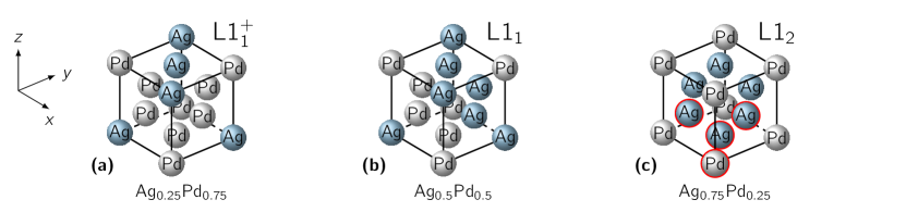
Figure 1: Schematic pictures of the three ordered structures found theoretically by Müller and Zunger [1] for the Ag concentration $c=0.25$, 0.5, and 0.75 ((a), (b) and (c), respectively). Only (c) depicts a unit cell (red circles indicate the basis atoms). L$1_{1}^{+}$ is formed of a Pd and a mixed Pd/Ag layer in [111] direction, whereas in L$1_{1}$, a Pd layer alternates with a full Ag layer in [111] direction.

1 Introduction

Short-range order (SRO), i.e., a partial degree of order within length scales comparable to interatomic distances, affects materials properties in many macroscopic ways. Its effects can be found in the optical conductivity and reflectivity [2, 3], magnetism [4], plasticity [5], and electronic structure [3, 6, 7, 8, 9]. A systematic study of SRO in Ag_cPd_1-c alloys is particularly informative, because their experimental phase diagram shows continuous solid solubility within the whole concentration range $c\in[0,1]$, in a randomly substitutional face centered cubic (fcc) structure [10]. Several theoretical predictions of stable long-range order (LRO), i.e., perfectly periodic, lower energy phases, have been also made in this system [1, 11]. These include in particular unit cell types L$1_{2}$, L$1_{1}$ and so-called L$1_{1}^{+}$ (a variation of the L$1_{1}$ case, with its original Ag layer hosting $50\text{\,}\mathrm{\char 37\relax}$ Pd atoms[1]) at $c=0.75$, $c=0.5$ and $c=0.25$, respectively (see figure 1).

The present study adds to our previous qualitative investigation of SRO effects on elastic and Fermi surface properties of Ag_cPd_1-c [12] a quantitative analysis of various degrees of SRO in Ag_cPd_1-c. The theoretical approach used in [12] – the multi-sublattice extension of the dynamical cluster approximation [13] / non-local coherent potential approximation (MS-NL-CPA) [14, 15] – extends the original single-site coherent potential approximation (CPA) allowing the evaluation of SRO modeled as local environments up to a given “cavity” size $N_{c}\times N_{\text{sub}}$. Here, $N_{\text{sub}}$ is the number of sublattices in a reference unit cell while $N_{c}$ counts multiple instances of that unit cell (so-called reciprocal space “tiles”). The SRO character of this approach is then included via the variation of a possible occupation of the sublattices by alternative atomic species. It is typically described through the introduction of a order parameter. One example of a SRO parameter, $\alpha$, is offered by the Warren-Cowley definition [16, 17], which has been previously used for proof-of-concept evaluations of SRO effects in CuZn alloys [14], in comparison with actual neutron scattering experiments on $\beta$ brass [18], and in the first-principles study of electrical conductivity [19, 20]. Temmermann et al[21] found from theoretical calculations that the order-disorder transformation in $\beta$ brass should be visible in photoemission spectra.

In this work, we further develop such parametrization of the SRO and target a more quantitative comparison with past experiments on Ag_cPd_1-c alloys. These alloys are on the one hand easy to handle model systems, since they show intermixing at variable concentrations, but might also stabilize in various geometrically periodic yet substitutionally disordered phases. On the other hand, practical reasons of interest for such compounds are given by possible application for fuel cells, catalysts, hydrogenation, sensors and biosensors and dental implantology [22]. Besides bulk properties, other areas of current interest entail the structure of Pd-Ag nanoparticles (see Ref. [23] and references therein).

We calculated the total density of states (DOS) for the different SRO settings and compared the predicted SRO changes with available experimental photoelectron spectroscopy (PES) data. Much more features, which would allow a specific fingerprint of a SRO scenario, were visible in the theoretical prediction than in the measured PES. Since the available experimental material is quite old and the present day high-resolution PES methods will allow better differentiation, we expect that changes in SRO will be traceable within PES experiments.

In the following section 2, we describe the adopted theoretical method in its essential details. The formulation of a suitably general SRO parameter is given in section 2.1. We use it in section 3 to compare between theoretical DOS results at different ordering regimes and the experimental peak positions from PES. Our conclusions are summarized in section 4.

2 Computational details

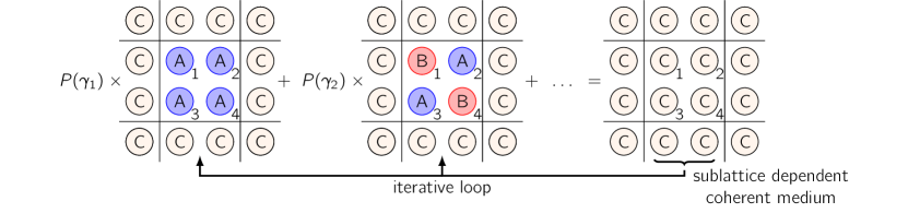
Figure 2: Schematic two-dimensional view of the MS-NL-CPA method for $N_{\text{sub}}=4$ and $N_{c}=1$. Numbers 1 to 4 mark the sublattice positions $s$.

The electronic structure calculation scheme of choice was the Korringa-Kohn-Rostoker Green’s function (KKR-GF) method. Here, the HUTSEPOT code developed by A. Ernst et al[24, 25] was used. We adopted the same calculation settings as used in our previous work [12]. Thus, the full charge density approximation (FCDA) was applied in order to describe the potentials properly and the local density approximation (LDA) [26] was used as exchange-correlation functional. The expansion cut-off for the spherical harmonics in the KKR-GF was set to $l_{\text{max}}=3$. Relaxed lattice parameters as a function of the concentration have been computed from total energy minimization through a fit to the Birch-Murnaghan equation of states [27, 28] (table 1).

Table 1: Calculated equilibrium lattice constants corresponding to the different alloy concentrations. The values are taken from CPA results [12].

• $c$	0.25	0.5	0.75
  $a_{\text{lat}}$ [$\mathrm{\SIUnitSymbolAngstrom}$]	3.890	3.929	3.970

Within the MS-NL-CPA framework, we describe the SRO considering a multi-site cavity, here set up with $N_{c}=1$ tiles but $N_{\text{sub}}\geq 1$ sublattices [15]. This situation is sketched in figure 2. Beginning from a starting assumption for the coherent medium, the calculation is iterated until self-consistency of the coherent medium. In general, if each disordered cavity site $s$ can host $N_{\text{a}}(s)$ alternative atomic species, there will be in total $N_{\text{tot}}=\prod_{s=1}^{N_{\text{sub}}}N_{a}^{N_{c}}(s)$ possible local configurations $\gamma$, each with weight $P(\gamma)$.

This framework allows to recover LRO results when only one, periodically repeated configuration occurs with probability one. On the opposite end, we obtain the fully uncorrelated scenario of a perfectly disordered lattice (which corresponds to the original single-site CPA picture) when all $\gamma$ are sampled with a probability distribution

$$P(\gamma)=\prod_{I=1}^{N_{c}}\prod_{s=1}^{N_{\text{sub}}}c_{A(I,s,\gamma)}\,,$$ (1)

only given by the factorized concentrations $c_{A(I,s,\gamma)}$. They represent the single-site concentration of an atomic species $A$ appearing on the (MS-)NL-CPA tile $I\in\{1,\ldots,N_{c}\}$ and the sublattice $s\in\{1,\ldots,N_{\text{sub}}\}$, when the cavity is populated by configuration $\gamma$. Intermediate scenarios can be described adopting alternative probability values $P(\gamma_{i})\in[0,1]$, which are subject to the normalization constraint

$$\sum_{i=1}^{N_{\text{tot}}}P(\gamma_{i})=1\,,$$ (2)

and satisfying the stoichiometry requirement for any atomic type $A$

$$\frac{1}{N_{c}N_{\text{sub}}}\sum_{i=1}^{N_{\text{tot}}}P(\gamma_{i})\times\mathcal{N}_{A}(\gamma_{i})=c_{A}\,.$$ (3)

Therein, the factor $\mathcal{N}_{A}(\gamma_{i})$ counts how many atoms of type $A$ appear within configuration $\gamma_{i}$.

We note that our results represent an upper limit for the influence of SRO effects on the physical effective medium, on top of those due to concentration alone. This originates from the $N_{c}$ coarse-graining subdivisions of the original Brillouin zone in reciprocal space [29], which are chosen consistently with the point group symmetries of the lattice but remain only defined up to a systematic offset (or “tiling phase factor” [29]) in the relative origin for the cluster momenta ${{\bi K}}_{n}$. At the moment, there is no systematic KKR-GF implementation of a corrective, additional sampling step for the tiling phase factor. Therefore, single tiling phase results - such as those discussed in the following - might slightly broaden, when including a proper phase average.

2.1 A general short-range order parameter

We intend to improve our previous work [12] with a quantitative description of SRO, and facilitate a comparison with experiments. To this end, we begin by recalling the Warren-Cowley SRO parameter definition [16, 17]. It is for a generic $A_{c},B_{1-c}$ binary alloy computed from the number $n_{l}$ of $A$ atoms found in the $l$-th shell around a $B$ atom

$$\alpha_{l}^{BA} =1-\frac{n_{l}}{c_{A}C_{l}}$$ (4)

$$=1-\frac{p^{BA}_{l}}{c_{A}}\,,$$ (5)

Therein, $C_{l}$ is the coordination number of the $l$-th shell around $B$ and the second expression is obtained by inserting the ratio $p^{BA}_{l}={n_{l}}/{C_{l}}$ of $A$ atoms within shell $l$ around a $B$ atom. Complex unit cell cases can be handled through an additional $N_{\text{sub}}$-normalized summation across sublattices.

When considering a (MS-)NL-CPA cavity, the SRO parameter (4) is deployed for each configuration $\gamma_{i}$, leading to the global result as a $P(\gamma_{i})$-weighted average. This general case can present some difficulties, since the shell radius in (4) may exceed the cavity size, so that the occupation of the considered lattice sites lies beyond the explicit listing of a configuration $\gamma_{i}$ (see figure 2, colored spheres are “inside” and C spheres are “outside” of the cavity). We propose therefore a general SRO parameter defined by the procedure below. Therein, it is convenient to introduce a generic occupation function $\sigma_{s}^{A}$ for each atomic species $A$, which returns a value “1”, if the crystalline position $s$ under examination hosts an $A$ atom, or “0”, if not. At every instance, an example is given with respect to the configuration $\gamma_{2}$ in figure 2 (middle panel) with $N_{\text{sub}}=4$ and $N_{c}=1$ (see also section 2.3).

1. As long as a sublattice remains fully contained within the explicit configuration, the constrained probability for $A$ to appear on sublattice $s$ of the (MS-)NL-CPA cavity cell $I$ is given by the occupation function $\sigma_{I,s}^{A}$. When instead a shell’s site lies beyond the cavity, its constrained probability becomes

   $$p^{A}_{\text{C}}(I,s) =\sum_{i=1}^{N_{\text{tot}}}P(\gamma_{i})\sigma_{I,s}^{A}\,.$$ (6)

   We note that in case of a disordered site, in the sense of the single-site CPA, $N_{\text{tot}}=1$ and the occupation function in (6) is substituted by a concentration.

   Example: Sites 1, 2, 3, and 4 are determined by $\gamma_{2}$ (inside the cavity), while all sites marked with C are not included in any configuration (outside the cavity).

2. The conditional probability in (5) for each configuration $\gamma_{i}$ and across the shell $l$ is computed by

   $$p^{BA}_{l}(\gamma_{i},I,s)=\frac{1}{C_{l}}\sum_{n=1}^{C_{l}}\cases{{p}_{A}(I,s)&\text{$n$ inside,}\\ \sigma_{I,s}^{A}&\text{$n$ outside,}\\ }$$ (7)

   where the $n=1,\ldots,C_{l}$ sites are either inside or outside the cavity.

   Example: Site 1 has four nearest neighbor sites. The probability of sites 2 and 3 is taken into account within $\gamma_{2}$ by $\sigma_{1,2}^{A}$ and $\sigma_{1,3}^{A}$, respectively, whereas the other two sites are outside and their probability is $p^{A}_{\text{C}}(1,2)$ and $p^{A}_{\text{C}}(1,3)$.

3. Using (7) in (5) yields the SRO parameter $\bar{\alpha}_{l}(\gamma_{i})$ as a function of the configuration $\gamma_{i}$. The arithmetic average is taken over all sublattices and tiles for the $l$-th shell (using $\alpha^{AB}_{l}(\gamma_{i},I,s)$ or $\alpha^{BA}_{l}(\gamma_{i},I,s)$).

   Example: Average over the sites 1, 2, 3 and 4.

4. In a final step, the SRO parameter per shell is derived via

   $$\alpha_{l}=\sum_{i=1}^{N_{\mathrm{tot}}}P(\gamma_{i})\times\bar{\alpha}_{l}(\gamma_{i})\,.$$ (8)

   Example: Take into account all other configurations and the corresponding $P(\gamma_{i})$ as well.

5. A possible average over the shells up to $N_{\text{sh}}$ may include weighting with the coordination number $C_{l}$ [30]

   $$\langle\alpha\rangle_{N_{\text{sh}}}=\Big{[}{\sum_{l=1}^{N_{\text{sh}}}C_{l}\times\alpha_{l}}\Big{]}\Big{/}\sum_{l=1}^{N_{\text{sh}}}C_{l}\,.$$ (9)

   However, $N_{\text{sh}}$ is not yet defined. Its value may depend on the lattice structure as discussed below in section 3.2. Thus, we restrict this study to the nearest neighbor SRO parameter.

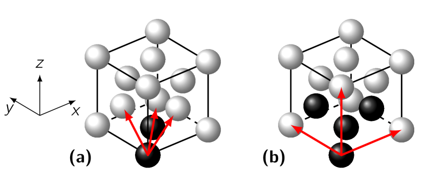
Figure 3: The used cells for the representation of the fcc lattice. (a) with two basis sites. (b) with 4 basis sites. Red arrows indicate the lattice vectors, and black spheres represent the basis sites.

2.2 Parameter space of the probabilities: an example

Although the definition of the SRO parameter consists only of different kinds of averages, the choice of the probabilities is still an open question. The connection of the SRO parameter with the probabilities can be only visualized for a simple test case, which contains only $N_{\text{sub}}=2$ sublattices with $N_{\text{tot}}=2^{2}=4$ possible configurations. Otherwise, the number of configurations becomes too large. Therefore, we begin at first to consider this $N_{\text{sub}}=2$ example for a lattice, which is described by the vectors ${{\bi R}}_{1}=(0,1/2,1/2)$, ${{\bi R}}_{2}=(1/2,0,1/2)$ and ${{\bi R}}_{3}=(1,1,0)$ and the basis vectors ${{\bi a}}_{1}=(0,0,0)$ and ${{\bi a}}_{2}=(1/2,1/2,0)$ (see figure 3a). This lattice structure resembles an fcc lattice.

The system of equations formed from (2) and (3) has only one solution and yields for the four probabilities

$$P(\gamma_{1})=P(\gamma_{4})\,,$$ (10)

$$P(\gamma_{2})=1-P(\gamma_{3})-2P(\gamma_{4})\,,$$ (11)

$$0\leq P(\gamma_{3})\leq 1\,,$$ (12)

$$0\leq P(\gamma_{4})\leq\frac{1-P(\gamma_{3})}{2}\,.$$ (13)

The two latter probabilities are free parameters. These allow a graphical analysis of the SRO parameter in a contour plot (see figure 4). The local variations inside the cavity determines only the nearest neighbor SRO parameter $\alpha_{1}$ (see figure 4a). It varies between $-\nicefrac{{1}}{{12}}$ and $+\nicefrac{{1}}{{12}}$. The highest degree of order is found for $P(\gamma_{3})=0.5$ and $P({\color[rgb]{0,0,0}\gamma_{4}})=0$, which means having the configurations (Pd Ag) and (Ag Pd) equally distributed. On the other hand, the highest degree of segregation in $\alpha_{1}$ is realized having $P(\gamma_{1})=P({\color[rgb]{0,0,0}\gamma_{4}})=0.5$.

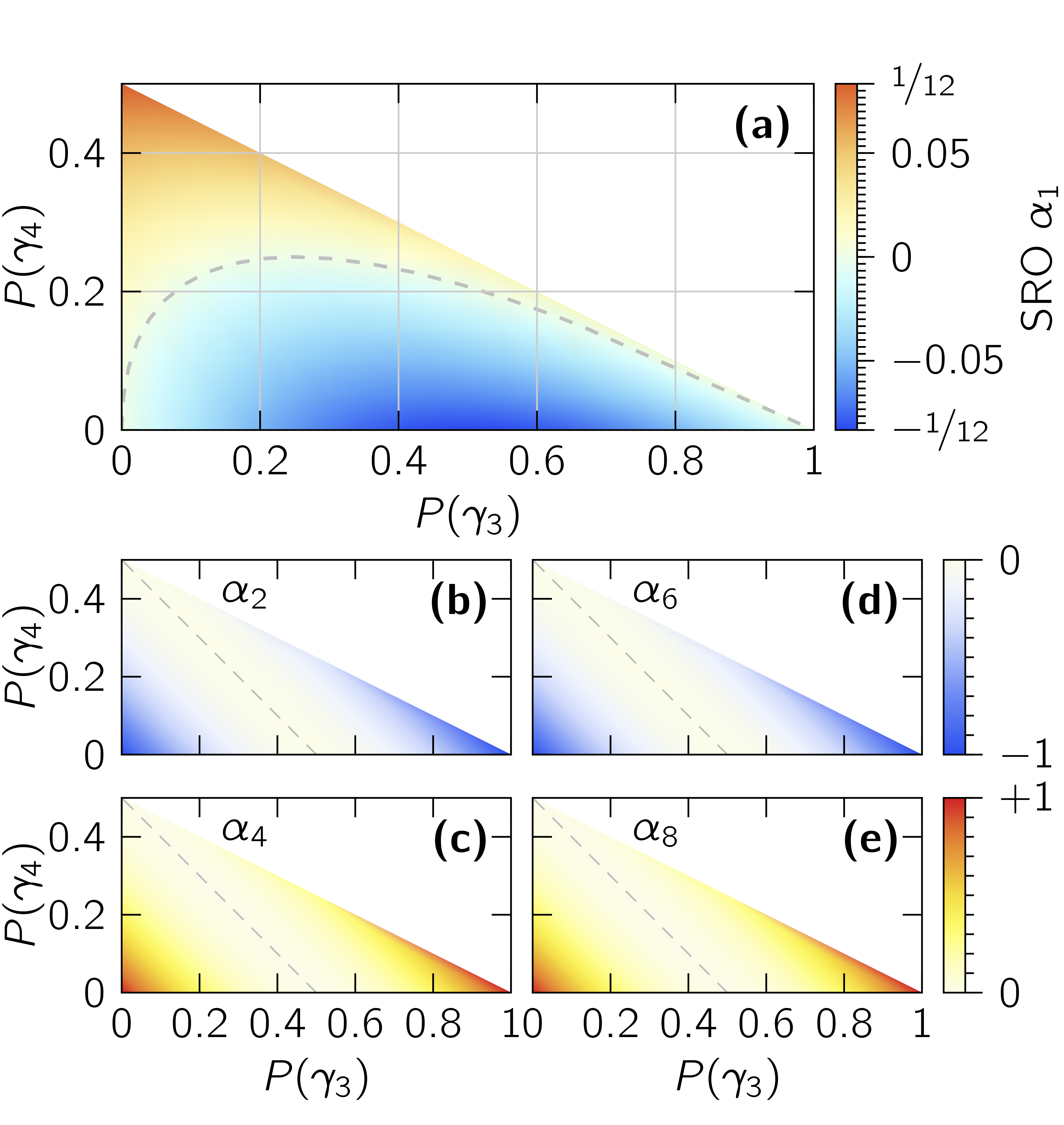
Figure 4: (a) The nearest neighbor SRO parameter $\alpha_{1}$, color coded as a function of the two probabilities $P(\gamma_{3})=P(\text{Pd\,Ag})$ and $P(\gamma_{4})=P(\text{Pd\,Pd})$. The triangle shape follows from the restrictions in (12) and (13). The dashed line indicates $\alpha_{1}=0$. (b)-(e) The SRO parameter for the following shells vary between $-1$ and $1$ and repeat themselves (see text). The SRO parameter not shown ($\alpha_{3}$, $\alpha_{5}$, $\alpha_{7}$) are completely zero.

The higher shells reflect the periodicity of the underlying lattice and the coherent medium (see figure 4b to 4e). Due to the choice of the lattice and basis vectors, the first period includes the shells until $l=5$. However, we restrict in this study the average of the SRO parameter to the non-periodic contribution, since this represents mainly the character of the SRO.

2.3 A reasonable choice of sublattices

Although the example demonstrates well the concept of the SRO parameter in the MS-NL-CPA, its configuration space is a little bit too restricted. Therefore, we considered a $N_{\text{sub}}=4$ sublattice supercell sketched in figure 3b (lattice vectors of a simple cubic cell with the basis of ${{\bi a}}_{1}=(0,0,0)$, ${{\bi a}}_{2}=(1/2,1/2,0)$, ${{\bi a}}_{3}=(1/2,0,1/2)$ and ${{\bi a}}_{4}=(0,1/2,1/2)$). In this case, the corresponding probabilities of the 16 potential configurations can not be parametrized by two free values.

Table 2: All 16 possibilities for the occupation of $N_{\text{sub}}=4$ sublattices in fcc Ag_cPd_1-c. The last column defines new probabilities $\tilde{P}(\mathcal{N}_{\text{Ag}}(\gamma_{i}))$.

• 	configurations $\gamma_{i}$
  $i$	${{\bi a}}_{1}$	${{\bi a}}_{2}$	${{\bi a}}_{3}$	${{\bi a}}_{4}$	$c_{\text{Ag}}$	$c_{\text{Pd}}$	$\mathcal{N}_{\text{Ag}}(\gamma_{i})$
  1	Ag	Ag	Ag	Ag	1	0	4	$\tilde{P}(4)$
  2	Ag	Ag	Ag	Pd	$\nicefrac{{3}}{{4}}$	$\nicefrac{{1}}{{4}}$	3	$\tilde{P}(3)$
  3	Ag	Ag	Pd	Ag	$\nicefrac{{3}}{{4}}$	$\nicefrac{{1}}{{4}}$	3
  4	Ag	Pd	Ag	Ag	$\nicefrac{{3}}{{4}}$	$\nicefrac{{1}}{{4}}$	3
  5	Pd	Ag	Ag	Ag	$\nicefrac{{3}}{{4}}$	$\nicefrac{{1}}{{4}}$	3
  6	Ag	Ag	Pd	Pd	$\nicefrac{{1}}{{2}}$	$\nicefrac{{1}}{{2}}$	2	$\tilde{P}(2)$
  7	Ag	Pd	Ag	Pd	$\nicefrac{{1}}{{2}}$	$\nicefrac{{1}}{{2}}$	2
  8	Ag	Pd	Pd	Ag	$\nicefrac{{1}}{{2}}$	$\nicefrac{{1}}{{2}}$	2
  9	Pd	Ag	Ag	Pd	$\nicefrac{{1}}{{2}}$	$\nicefrac{{1}}{{2}}$	2
  10	Pd	Ag	Pd	Ag	$\nicefrac{{1}}{{2}}$	$\nicefrac{{1}}{{2}}$	2
  11	Pd	Pd	Ag	Ag	$\nicefrac{{1}}{{2}}$	$\nicefrac{{1}}{{2}}$	2
  12	Ag	Pd	Pd	Pd	$\nicefrac{{1}}{{4}}$	$\nicefrac{{3}}{{4}}$	1	$\tilde{P}(1)$
  13	Pd	Ag	Pd	Pd	$\nicefrac{{1}}{{4}}$	$\nicefrac{{3}}{{4}}$	1
  14	Pd	Pd	Ag	Pd	$\nicefrac{{1}}{{4}}$	$\nicefrac{{3}}{{4}}$	1
  15	Pd	Pd	Pd	Ag	$\nicefrac{{1}}{{4}}$	$\nicefrac{{3}}{{4}}$	1
  16	Pd	Pd	Pd	Pd	0	1	0	$\tilde{P}(0)$

However, the restrictions in (2) and (3) depend only on the number of $A$ or $B$ types in each configuration (internal concentration), whereby several configurations have an equal number of atomic types, which occupy only different sublattices (see table 2). A new probability $\tilde{P}(\mathcal{N}_{\text{Ag}}(\gamma_{i}))$ is assigned to every group depending on the number of Ag atoms $\mathcal{N}_{\text{Ag}}(\gamma_{i})$. With these 5 probabilities, the system of equations (2) and (3) can be solved again, where two probabilities are determined by the others (see A). In fact, each $\tilde{P}(\mathcal{N}_{\text{Ag}}(\gamma_{i}))$ describes a subset of configurations, e.g., $\tilde{P}(3)$ condenses four configurations ($\gamma_{2}$ to $\gamma_{5}$), each having one Pd occupying another sublattice while the three sublattices left are occupied with Ag. Then, the probabilities $P(\gamma_{2})$, $P(\gamma_{3})$, $P(\gamma_{4})$, and $P(\gamma_{5})$ are free to choose but have to sum up to $\tilde{P}(3)$, otherwise violating the total concentration.

2.4 Comparison with experimental PES

We compare below our calculations of the DOS for different SRO regimes with experimental valence band PES of Ag-Pd alloys by McLachlan et al[31]. The mean positions of the experimentally observed spectral peaks are considered as the electron binding energies and are given in table 3. We preferred in particular the experimental He II ($40.81\text{\,}\mathrm{eV}$) spectra. Although the He II technique is in general rather surface sensitive, we expect that its application to metals with a highly efficient electronic screening can lead to useful insights on the bulk properties from analysis of the spectra. This is further confirmed by comparison of the specific He II results used in this study against the calculated XPS spectra of Winter et al[32], and the typical probing depth of about $50\text{\,}\mathrm{\SIUnitSymbolAngstrom}$ reported in experiments by Caroli et al[33], thus including substantial bulk contributions.

Table 3: Binding energies (in $\mathrm{eV}$, relative to the Fermi energy) of the main spectral peaks estimated from the experimental (He II) spectra by McLachlan et al[31] and interpolated to the concentrations used in the present calculations. The upper two rows are for the Pd $4d$ section of the spectrum and the lower two rows belong to the Ag $4d$ section.

• Ag0.25Pd0.75	Ag0.50Pd0.50	Ag0.75Pd0.25
  $0.5$	$1.0$	$1.4$
  $2.4$	$2.3$	$-$
  $4.9$	$4.6$	$4.4$
  $5.5$	$5.7$	$6.0$

3 Results

3.1 Broadening of the theoretical spectrum

When comparing theoretical DOS data with experimental results, the experimental resolution broadens the measured spectra and may hide some spectral features. The experimental resolution in the study of McLachlan et al[31] is given by $\pm$0.3\text{\,}\mathrm{eV}$$. However, in the modern high-resolution photoelectron measurement equipment, the energy resolution can go down to the range of few $\mathrm{meV}$ at low temperatures around $10\text{\,}\mathrm{K}$ [34, 35]. The influence of the experimental resolution on the calculated DOS can be simulated by the convolution of the DOS with a Gaussian. The resolution is understood as the full width at half maximum (FWHM) and is translated to the standard deviation $\sigma$ of the Gaussian distribution by $\text{FWHM}=2\sqrt{2\ln{2}}\sigma$.

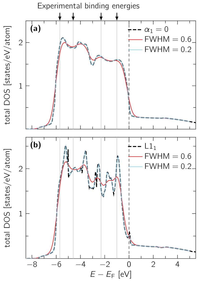
Figure 5: Calculated density of states of Ag_0.5Pd_0.5 convoluted with a Gaussian of different FWHM in order to simulate the experimental resolution. Two cases of SRO are depicted (a) $\alpha_{1}=0$ and (b) the ordered L$1_{1}$ structure. The binding energies of the main spectral peaks of the experimental PES (table 3) are highlighted by arrows and vertical gray lines. The spectra for the high experimental resolution ($\text{FWHM}=0.2$, blue line) and the purely theoretical spectra (black dashed line) lie almost on top of each other.

For two extreme SRO regimes, $\alpha_{1}=0$ (totally uncorrelated) and the L$1_{1}$ structure (order), the calculated and broadened DOS are depicted in figure 5. The first choice of $\text{FWHM}=0.6$ (red solid lines) corresponds to the resolution of the older experiment [31], whereas the $\text{FWHM}=0.2$ (light blue lines) matches with modern resolutions at room temperature. Already the latter resolution is sufficient to represent all significant peaks in the calculated DOS (black dashed line), even for the spiky DOS of the ordered structure (see figure 5b). It shows that this resolution would be in principle enough to differentiate between different SRO regimes with the combination of first-principles calculations and PES measurements. This is difficult with the older resolution, since the number of peaks and their variation is hardly distinguishable for the two examples $\alpha_{1}=0$ and L$1_{1}$ (compare red lines in figure 5). A comparison with the experimental peak position (see table 3) does not reveal a clear conclusion about the particular state of order.

3.2 Varying the short-range order

As a second step, we varied the degree of SRO at the Ag_cPd_1-c alloy concentrations $c=0.25$, $0.50$, $0.75$. We started with only 5 representative configurations of table 2, in particular 1, 2, 6, 12, 16, and varied the three probabilities, which are the free parameters (see A), in steps of 0.05. The obtained SRO parameter showed again a periodicity as already discussed in section 2.2. We chose several SRO parameter values and calculated the valence DOS. The results in dependence of the nearest neighbor SRO parameter $\alpha_{1}$ and for the ordered structures are depicted in figure 6, 7 and 8, respectively. The three figures show significant changes in the DOS with varying SRO. Some spectral peaks vanish, move or grow. Such strong variations should be easily visible in nowadays PES measurements.

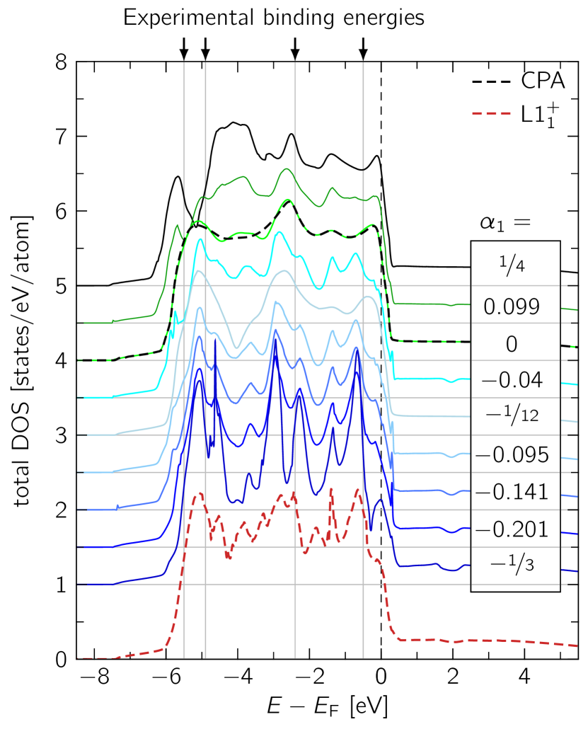
Figure 6: Calculated density of states of Ag_0.25Pd_0.75 for different degrees of nearest neighbor SRO $\alpha_{1}$, beginning with the ordered L$1_{1}^{+}$ structure. The corresponding configurations used for the SRO parameter are given in table 4. An offset is added to the curves (horizontal gray line represents zero). The binding energies of the main spectral peaks of the experimental PES (table 3) are highlighted by arrows and vertical gray lines.

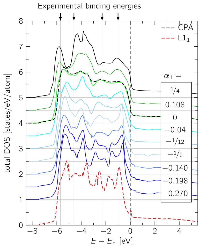
Figure 7: Calculated density of states of Ag_0.5Pd_0.5 for different degrees of nearest neighbor SRO $\alpha_{1}$, beginning with the ordered L$1_{1}$ structure. The corresponding configurations used for the SRO parameter are given in table 5. An offset is added to the curves (horizontal gray line represents zero). The binding energies of the main spectral peaks of the experimental PES (table 3) are highlighted by arrows and vertical gray lines.

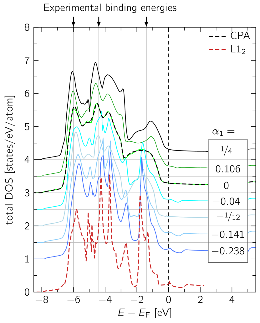
Figure 8: Calculated density of states of Ag_0.75Pd_0.25 for different degrees of nearest neighbor SRO $\alpha_{1}$, beginning with the ordered L$1_{2}$ structure. The corresponding configurations used for the SRO parameter are given in table 6. An offset is added to the curves (horizontal gray line represents zero). The binding energies of the main spectral peaks of the experimental PES (table 3) are highlighted by arrows and vertical gray lines.

When going from the ordered regime ($\alpha_{1}<0$) via the totally uncorrelated case ($\alpha_{1}=0$) towards the segregation behavior ($\alpha_{1}>0$), the spiky structure of the DOS looses its contrast and becomes smoother. Simultaneously, the band width is enhanced with increasing $\alpha_{1}$. Additionally, the experimental binding energies (see table 3) are indicated within the figure 6, 7 and 8 with arrows and thin gray lines. Although it became obvious in section 3.1 that a direct comparison between the experimental and theoretical results is hardly possible, the binding energies can at least be related with some pronounced peaks in the DOS and may offer a crude estimation of possible SRO scenarios.

For Ag_0.25Pd_0.75, the best agreement with the binding energies would be achieved with the assumption of a slight tendency of SRO around $\alpha_{1}=0$, since the double peak structure of the binding energies in the lower energy spectrum may hint to additional features coming from SRO (see figure 6). Nevertheless, the variation in the amount of SRO in Ag_0.25Pd_0.75 visualizes the gradually collapse or development of several spectral peaks when going from negative to positive $\alpha_{1}$. The minimal value for $\alpha_{1}$ is $-\nicefrac{{1}}{{3}}$ and represents again the L$1_{2}$ structure (but now, a Ag atoms at the corner and a Pd atom at the face of the cube). In contrast, L$1_{1}^{+}$ was found to be energetically more favorable but has a lower degree of ordering in terms of $\alpha_{1}$ ($\alpha_{1}=-\nicefrac{{1}}{{9}}$, $\alpha_{2}=-\nicefrac{{1}}{{3}}$, $\alpha_{3}=-\nicefrac{{1}}{{9}}$, $\ldots$). The averaged SRO parameters are $\langle\alpha\rangle_{2}=-\nicefrac{{5}}{{27}}\approx-0.185$ or $\langle\alpha\rangle_{3}=-\nicefrac{{1}}{{7}}\approx-0.143$. The different amount of SRO in L$1_{2}$ or L$1_{1}^{+}$ is directly visible in the DOS of both structures (see the dark blue line or the red dashed line in figure 6). While the DOS of L$1_{2}$ ($\alpha_{1}=-\nicefrac{{1}}{{3}}$) yielded sharper spectral peaks, the DOS of L$1_{1}^{+}$ matches better between $\alpha_{1}=-0.141$ and $\alpha_{1}=-0.201$.

The analysis of the DOS for Ag_0.5Pd_0.5 is quite similar as for Ag_0.25Pd_0.75. Several spectral peaks become wider and shift their positions (see figure 7). Also for this concentration, the proposed ordered structure L$1_{1}$ has not the lowest possible SRO parameter (minimum is $\alpha_{1}=-1$, but for L$1_{1}$ is $\alpha_{1}=0$, $\alpha_{2}=-1$, $\alpha_{3}=0$, $\alpha_{4}=1$, $\ldots$). The DOS does not seem to fit well in respect of the other DOS of the remaining SRO scenarios. The symmetric cubic cell with $N_{\text{sub}}=4$ might not be the best choice of comparing with the layered structure of L$1_{1}$. In terms of the experimental binding energies, the SRO regime of $\alpha_{1}=0$ agrees best with the theoretically calculated number of spectral peaks and their positions.

When further raising the concentration of Ag to Ag_0.75Pd_0.25, the SRO related widening of the spectral peaks observed for the ordered structure L$1_{2}$ can be traced (see energy range between $-2\text{\,}\mathrm{eV}0\text{\,}\mathrm{eV}$ in figure 8). L$1_{2}$ ($\alpha_{1}=-\nicefrac{{1}}{{3}}$) has already the lowest possible SRO parameter and is described well by the small cubic cell. Thus, all spectral peaks obtained for L$1_{2}$ just loose their height and become broader, if the SRO is varied towards $\alpha_{1}=0$. The comparison with the experimental binding energies at $c=0.75$ indicates again a mostly disordered sample representing the crucial peaks in the theoretical spectrum well (see arrows in figure 8).

The good description of the $c=0.75$ case within the $N_{\text{sub}}=4$ supercell (see figure 3) is also verified by calculated total energies. Thereby, the L$1_{2}$ structure had the lowest total energy and the total energy increased just linearly (not shown) when varying the degree of SRO. However for the other two concentrations, there was no clear tendency visible. Only the respective ordered structures – L$1_{1}$ and L$1_{1}^{+}$ – had the lowest total energies.

Finally, the calculated DOS at $c=0.25$, $0.5$ and $0.75$ were also compared with the PES measurements of Norris and Nilsson [36], Hüfner et al[37, 38], Chae et al[39] and Traditi et al[40]. In general, the experimental spectra agree best with the DOS of the random ($\alpha_{1}=0$) or the ordering ($\alpha_{1}<0$) cases, while the clustering features ($\alpha_{1}>0$) are less probable. This is in agreement with the complete solubility of Ag and Pd at ambient temperatures and with the ordering tendency at low temperatures [1].

4 Conclusions

The SRO induced changes in the DOS are significantly larger than the typical energy resolution in the valence band PES measurements [31]. We have demonstrated that the SRO phenomena in alloys can be in principle discernible in valence band photoelectron spectra. With proper SRO calculations, e.g., within the MS-NL-CPA, the experimental PES data can be used to determine the type of the prevailing SRO. Thus, the PES technique can be considered as one potential experimental method to investigate SRO structures of alloys.

Comparing our MS-NL-CPA valence DOS of Pd-Ag alloys with existing PES measurements suggests that the SRO in the measured Pd-Ag samples has been in most cases that of uncorrelated disorder with some traces of ordering. Nevertheless, PES measurements with resolution available in modern technique would be beneficial to get more definite information of SRO in Pd-Ag alloys.

Appendix A Relation between probabilities

The redefined probabilities $\tilde{P}(\mathcal{N}_{\text{Ag}}(\gamma_{i}))$ form a similar system of equations as (2) and (3)

$$\tilde{P}(4)+\nicefrac{{3}}{{4}}\tilde{P}(3)+\nicefrac{{1}}{{2}}\tilde{P}(2)+\nicefrac{{1}}{{4}}\tilde{P}(1) =c\,,$$ (14)

/14$$\tilde{P}(3)+\nicefrac{{1}}{{2}}\tilde{P}(2)+\nicefrac{{3}}{{4}}\tilde{P}(1)+\tilde{P}(0) =1-c\,,$$ (15)

$$\sum_{i}^{4}\tilde{P}(i)=1\,,$$ (16)

$$0\leq\tilde{P}(i)\leq 1\,,$$ (17)

where $c=c_{\text{Ag}}$ and $1-c=c_{\text{Pd}}$. This system of equations has, in particular for $c=0.5$, a solution where the parameter space is spanned by $\tilde{P}(2)$, $\tilde{P}(3)$, and $\tilde{P}(4)$, under the conditions

$$\big{(}2\tilde{P}(2)+3\tilde{P}(3)+4\tilde{P}(4)\leq 2\big{)}\wedge$$

$$\bigg{\{}\big{[}\big{(}\tilde{P}(2)+2\tilde{P}(3)+3\tilde{P}(4)\geq 1\big{)}\wedge\big{(}\tilde{P}(2)+2\tilde{P}(3)\leq 1\big{)}\big{]}\vee$$

$$\big{[}\big{(}\tilde{P}(2)+2\tilde{P}(3)\geq 1\big{)}\wedge\big{(}2\tilde{P}(2)+3\tilde{P}(3)\leq 2\big{)}\big{]}\bigg{\}}\,.$$ (18)

The remaining probabilities are then given by

$$\tilde{P}(0)=\tilde{P}(2)+2\tilde{P}(3)+3\tilde{P}(4)-1\,,$$ (19)

$$\tilde{P}(1)=2-2\tilde{P}(2)-3\tilde{P}(3)-4\tilde{P}(4)\,.$$ (20)

If $\tilde{P}(4)$ is zero, a simple solution follows from (18)

$$\tilde{P}(0) =\frac{1-\tilde{P}(2)}{3}\,,$$ (21)

$$\tilde{P}(1) =\tilde{P}(4)=0\,,$$ (22)

$$\tilde{P}(3) =-\frac{2(\tilde{P}(2)-1)}{3}\,,$$ (23)

while $0\leq\tilde{P}(2)\leq 1$ is the only free parameter. The conditions and probabilities for the other concentrations $c=0.25$ and $0.75$ can be found following a similar procedure.

Table 4: Nearest neighbor SRO parameter and the corresponding configurations used for fcc Ag_0.25Pd_0.75 with $N_{\text{sub}}=4$. For $\alpha=0$, all 16 configurations are used and their probabilities are given by (1).

• 		Probabilities $P(\gamma_{i})$ for $\alpha_{1}=$
  confs.	$c_{\text{Ag}}$	$-\nicefrac{{1}}{{3}}$	$-0.201$	$-0.141$	$-0.095$	$-\nicefrac{{1}}{{12}}$	$-0.04$	$0.099$	$\nicefrac{{1}}{{4}}$
  1 1 1 1	$1$	$0$	$0$	$0.05$	$0.05$	$0$	$0.1$	$0.15$	/14
  1 1 1 0	$\nicefrac{{3}}{{4}}$	$0$	$0.05$	$0$	$0.05$	$0$	$0$	$0$	$0$
  1 1 0 0	$\nicefrac{{1}}{{2}}$	$0$	$0.05$	$0.05$	$0$	/16	$0$	$0.05$	$0$
  1 0 0 0	$\nicefrac{{1}}{{4}}$	$1$	/34	$0.7$	$0.65$	/14	$0.6$	$0.3$	$0$
  0 1 0 0	$\nicefrac{{1}}{{4}}$	$0$	$0$	$0$	$0$	/14	$0$	$0$	$0$
  0 0 1 0	$\nicefrac{{1}}{{4}}$	$0$	$0$	$0$	$0$	/14	$0$	$0$	$0$
  0 0 0 1	$\nicefrac{{1}}{{4}}$	$0$	$0$	$0$	$0$	/14	$0$	$0$	$0$
  0 0 0 0	$0$	$0$	$0.15$	$0.2$	/14	$0$	$0.3$	/12	/34

Table 5: Nearest neighbor SRO parameter and the corresponding configurations used for fcc Ag_0.5Pd_0.5 with $N_{\text{sub}}=4$. For $\alpha=0$, all 16 configurations are used and their probabilities are given by (1).

• 		Probabilities $P(\gamma_{i})$ for $\alpha_{1}=$
  confs.	$c_{\text{Ag}}$	$-0.270$	-0.198	$-0.140$	$-\nicefrac{{1}}{{9}}$	$-\nicefrac{{1}}{{12}}$	-0.04	0.108	$\nicefrac{{1}}{{4}}$
  1 1 1 1	1	0	0.1	0	0	0	0.2	0.3	$\nicefrac{{1}}{{2}}$
  1 1 1 0	$\nicefrac{{3}}{{4}}$	0.05	0	0.15	0	0	0	0.1	0
  1 1 0 1	$\nicefrac{{3}}{{4}}$	0.05	0	0.15	0	0	0	0	0
  1 1 0 0	$\nicefrac{{1}}{{2}}$	0.8	0.7	0.5	0	$\nicefrac{{1}}{{6}}$	0.6	0.2	0
  1 0 1 0	$\nicefrac{{1}}{{2}}$	0	0	0	0	$\nicefrac{{1}}{{6}}$	0	0	0
  1 0 0 1	$\nicefrac{{1}}{{2}}$	0	0	0	$\nicefrac{{1}}{{3}}$	$\nicefrac{{1}}{{6}}$	0	0	0
  0 1 1 0	$\nicefrac{{1}}{{2}}$	0	0	0	0	$\nicefrac{{1}}{{6}}$	0	0	0
  0 1 0 1	$\nicefrac{{1}}{{2}}$	0	0	0	$\nicefrac{{1}}{{3}}$	$\nicefrac{{1}}{{6}}$	0	0	0
  0 0 1 1	$\nicefrac{{1}}{{2}}$	0	0	0	$\nicefrac{{1}}{{3}}$	$\nicefrac{{1}}{{6}}$	0	0	0
  1 0 0 0	$\nicefrac{{1}}{{4}}$	0.1	0.2	0.1	0	0	0	0.1	0
  0 0 0 0	0	0	0	0.1	0	0	0.2	0.3	$\nicefrac{{1}}{{2}}$

Appendix B Used configurations and probabilities

The configurations and probabilities used to calculate the DOS shown in figure 6 to 8 are presented in table 4, 5, and 6, respectively. Besides, the 5 representative configurations indicated in table 2, we chose also additional configurations in order to test the method.

Table 6: Nearest neighbor SRO parameter and the corresponding configurations used for fcc Ag_0.75Pd_0.25 with $N_{\text{sub}}=4$. For $\alpha=0$, all 16 configurations are used and their probabilities are given by (1).

• 		Probabilities $P(\gamma_{i})$ for $\alpha_{1}=$
  confs.	$c_{\text{Ag}}$	-0.238	-0.141	$-\nicefrac{{1}}{{12}}$	-0.04	0.106	$\nicefrac{{1}}{{4}}$
  1 1 1 1	1	01	0.2	0	0.3	0.6	$\nicefrac{{3}}{{4}}$
  1 1 1 0	$\nicefrac{{3}}{{4}}$	0.85	0.7	$\nicefrac{{1}}{{4}}$	0.6	0.1	0
  1 1 0 1	$\nicefrac{{3}}{{4}}$	0	0	$\nicefrac{{1}}{{4}}$	0	0	0
  1 0 1 1	$\nicefrac{{3}}{{4}}$	0	0	$\nicefrac{{1}}{{4}}$	0	0	0
  0 1 1 1	$\nicefrac{{3}}{{4}}$	0	0	$\nicefrac{{1}}{{4}}$	0	0	0
  1 1 0 0	$\nicefrac{{1}}{{2}}$	0	0.05	0	0	0.05	0
  1 0 0 0	$\nicefrac{{1}}{{4}}$	0.05	0	0	0	0.2	0
  0 0 0 0	0	0	0.05	0	0.1	0.05	$\nicefrac{{1}}{{4}}$

Bibliography

Bibliography

- [1] Müller S and Zunger A 2001 Phys. Rev. Lett. 87 165502 URL http://link.aps.org/doi/10.1103/PhysRevLett.87.165502
- [2] Mookerjee A, Tarafder K, Chakrabarti A and Saha K K 2008 Pramana 70 221 URL http://link.springer.com/10.1007/s12043-008-0041-0
- [3] Jezierski A 1993 Phys. Status Solidi B 178 373 URL http://doi.wiley.com/10.1002/pssb.2221780213
- [4] Parra R E and González A C 1999 J. Appl. Phys. 85 4735 URL http://scitation.aip.org/content/aip/journal/jap/85/8/10.1063/1.370464
- [5] Jiang M and Dai L 2010 Phil. Mag. Lett. 90 269 URL http://www.tandfonline.com/doi/abs/10.1080/09500831003630781
- [6] Staunton J B, Johnson D D and Pinski F J 1994 Phys. Rev. B 50 1450 URL http://link.aps.org/doi/10.1103/PhysRevB.50.1450
- [7] Wahrenberg R, Stupp H, Boyen H G and Oelhafen P 2000 Europhys. Lett. 49 782 URL http://stacks.iop.org/0295-5075/49/i=6/a=782?key=crossref.79304febbde6c90dc4e468daf18f180b
- [8] Golovchak R, Shpotyuk O, Kozyukhin S, Shpotyuk M, Kovalskiy A and Jain H 2011 J. Non-Cryst. Solids 357 1797 URL http://linkinghub.elsevier.com/retrieve/pii/S0022309311001244
- [9] Novikov Y N and Gritsenko V A 2011 J. Appl. Phys. 110 014107 URL http://scitation.aip.org/content/aip/journal/jap/110/1/10.1063/1.3606422
- [10] Hultgren R, Desai P D, Hawkins D T, Gleiser M and Kelley K K 1973 Selected Values of the Thermodynamic Properties of Binary Alloys (Metals Park, Ohio: American Society for Metals)
- [11] Ruban A V, Simak S I, Korzhavyi P A and Johansson B 2007 Phys. Rev. B 75 054113 URL http://link.aps.org/doi/10.1103/PhysRevB.75.054113
- [12] Hoffmann M, Marmodoro A, Nurmi E, Kokko K, Vitos L, Ernst A and Hergert W 2012 Phys. Rev. B 86 094106 URL http://prb.aps.org/abstract/PRB/v86/i9/e094106
- [13] Jarrell M and Krishnamurthy H R 2001 Phys. Rev. B 63 125102 URL http://link.aps.org/doi/10.1103/PhysRevB.63.125102
- [14] Rowlands D A, Ernst A, Györffy B L and Staunton J B 2006 Phys. Rev. B 73 165122 URL http://link.aps.org/doi/10.1103/PhysRevB.73.165122
- [15] Marmodoro A, Ernst A, Ostanin S and Staunton J B 2013 Phys. Rev. B 87 125115 URL http://link.aps.org/doi/10.1103/PhysRevB.87.125115
- [16] Cowley J M 1950 Phys. Rev. 77 669 URL http://link.aps.org/doi/10.1103/PhysRev.77.669
- [17] Warren B E 1990 X-ray diffraction (New York: Dover Publications, Inc.) ISBN 978-0-486-66317-3 URL http://store.doverpublications.com/0486663175.html
- [18] Walker C B and Keating D T 1963 Phys. Rev. 130 1726 URL http://link.aps.org/doi/10.1103/PhysRev.130.1726
- [19] Butler W H and Stocks G M 1984 Phys. Rev. B 29 4217 URL http://journals.aps.org/prb/abstract/10.1103/PhysRevB.29.4217
- [20] Lowitzer S, Ködderitzsch D, Ebert H, Tulip P R, Marmodoro A and Staunton J B 2010 Europhys. Lett. 92 37009 URL http://stacks.iop.org/0295-5075/92/i=3/a=37009?key=crossref.b531c594f4591737a5caac4611899882
- [21] Temmerman W M, Durham P J, Szotek Z, Sob M and Larsson C G 1988 J. Phys. F: Met. Phys. 18 2387 URL http://stacks.iop.org/0305-4608/18/i=11/a=012?key=crossref.c0c0131d930fbe875a0d309e5bd8e0e9
- [22] Li D, Baba N, Brantley W A, Alapati S B, Heshmati R H and Daehn G S 2010 J. Mater. Sci. Mater. Med. 21 2723 URL http://www.ncbi.nlm.nih.gov/pubmed/20623178
- [23] Kozlov S M, Kovács G, Ferrando R and Neyman K M 2015 Chem. Sci. 6 3868 URL http://pubs.rsc.org/en/content/articlehtml/2015/sc/c4sc03321c
- [24] Ernst A 2007 Multiple-scattering theory: new developments and applications Cumulative habilitation Martin Luther University Halle-Wittenberg
- [25] Lüders M, Ernst A, Temmerman W M, Szotek Z and Durham P J 2001 J. Phys.: Condens. Matter 13 8587 URL http://stacks.iop.org/0953-8984/13/i=38/a=305
- [26] Perdew J P and Wang Y 1992 Phys. Rev. B 45 13244 URL http://link.aps.org/doi/10.1103/PhysRevB.45.13244
- [27] Birch F 1947 Phys. Rev. 71 809 URL http://link.aps.org/doi/10.1103/PhysRev.71.809
- [28] Poirier J P 2000 Introduction to the Physics of the Earth’s Interior 2nd ed (Cambridge: Cambridge University Press) ISBN 978-0-521-66392-2 URL http://www.cambridge.org/de/academic/subjects/earth-and-environmental-science/solid-earth-geophysics/introduction-physics-earths-interior-2nd-edition?format=PB
- [29] Rowlands D A, Zhang X G and Gonis A 2008 Phys. Rev. B 78 115119 URL http://link.aps.org/doi/10.1103/PhysRevB.78.115119
- [30] Mirebeau I, Hennion M and Parette G 1984 Phys. Rev. Lett. 53 687 URL http://link.aps.org/doi/10.1103/PhysRevLett.53.687
- [31] McLachlan A D, Jenkin J G, Leckey R C G and Liesegang J 1975 J. Phys. F: Met. Phys. 5 2415 URL http://iopscience.iop.org/0305-4608/5/12/028
- [32] Winter H, Durham P J and Stocks G M 1984 J. Phys. F: Met. Phys. 14 1047 URL http://stacks.iop.org/0305-4608/14/i=4/a=025
- [33] Caroli C, Lederer-Rozenblatt D, Roulet B and Saint-James D 1973 Phys. Rev. B 8 4552 URL http://link.aps.org/doi/10.1103/PhysRevB.8.4552
- [34] Hüfner S, Claessen R, Reinert F, Straub T, Strocov V and Steiner P 1999 J. Electron. Spectrosc. Relat. Phenom. 100 191 URL http://linkinghub.elsevier.com/retrieve/pii/S036820489900047X
- [35] Stadnik Z M, Purdie D, Baer Y and Lograsso T A 2001 Phys. Rev. B 64 214202 URL http://link.aps.org/doi/10.1103/PhysRevB.64.214202
- [36] Norris C and Nilsson P 1968 Solid State Commun. 6 649 URL http://dx.doi.org/10.1016/0038-1098(68)90186-5
- [37] Hüfner S, Wertheim G K and Wernick J H 1973 Phys. Rev. B 8 4511 URL http://link.aps.org/doi/10.1103/PhysRevB.8.4511
- [38] Hüfner S, Wertheim G and Wernick J 1975 Solid State Commun. 17 1585 URL http://dx.doi.org/10.1016/0038-1098(75)91001-7
- [39] Chae K, Lee Y, Whang C, Jeon Y, Choi B and Croft M 1996 Nucl. Instr. Meth. Phys. Res. B 117 123 URL http://dx.doi.org/10.1016/0168-583X(96)00293-5
- [40] Tarditi A, Bosko M and Cornaglia L 2012 Int. J. Hydrogen Energy 37 6020 URL http://dx.doi.org/10.1016/j.ijhydene.2011.12.128