Bypass transition and spot nucleation in boundary layers

Abstract

The spatio-temporal aspects of the transition to turbulence are considered in the case of a boundary layer flow developing above a flat plate exposed to free-stream turbulence. Combining results on the receptivity to free-stream turbulence with the nonlinear concept of a transition threshold, a physically motivated model suggests a spatial distribution of spot nucleation events. To describe the evolution of turbulent spots a probabilistic cellular automaton is introduced, with all parameters directly fitted from numerical simulations of the boundary layer. The nucleation rates are then combined with the cellular automaton model, yielding excellent quantitative agreement with the statistical characteristics for different free-stream turbulence levels. We thus show how the recent theoretical progress on transitional wall-bounded flows can be extended to the much wider class of spatially developing boundary-layer flows.

I Introduction

The boundary layers that form whenever a fluid flows over a solid surface determine many physical properties such as the drag on the surface or the transfer of heat (Schlichting, 2004). The theory for the laminar boundary layer was developed by Prandtl and Blasius, who described the velocity profile and the characteristic downstream variation of the boundary layer. The transition to a turbulent boundary layer is accompanied by dramatic changes in its physical properties, and remains a fascinating object of study because it often does not follow the linear instability described by Tollmien and Schlichting. Instead, finite amplitude perturbations can trigger turbulence much more quickly in a process dubbed bypass transition, so named to indicate that it circumvents the linear instability (Schmid and Henningson, 2001). The transitional region of the boundary layer is characterized by spatially and temporally fluctuating turbulent spots with an increasing probability to be turbulent farther downstream (Emmons, 1951; Klebanoff et al., 1962).

A key quantity in the characterization of the transition is the intermittency factor $\gamma(x)$, defined as the probability to be turbulent at streamwise position $x$. Most models that have been developed for $\gamma$ contain phenomenological assumptions about the nucleation rate of spots and their further evolution (Emmons, 1951; Dhawan and Narasimha, 1957; Narasimha, 1985; Johnson and Ercan, 1999; Vinod and Govindarajan, 2004, 2007). An exception is the model described in (Ustinov, 2013), where transient amplification of perturbations and a threshold for the transition are used to derive a dynamical model for the spot nucleation rate and hence $\gamma$. Other properties of the dynamics, such as the number and width of turbulent regions, are not considered. The model we describe here is based on our understanding of the transition in internal flows and contains a cellular automaton representation of the dynamics that also captures the time evolution of the spots.

The transition to turbulence in parallel flows such as plane Couette flow or pipe flow (Wygnanski and Champagne, 1973; Lundbladh and Johansson, 1991; Avila et al., 2011) shares many features with bypass transition in the spatially developing boundary layer (Emmons, 1951; Vinod and Govindarajan, 2004). In both sets of flows the laminar profile is conditionally stable and finite perturbations are needed to trigger the transition. In the case of parallel flows, the transition to turbulence has been linked to the appearance of 3-D exact coherent structures via saddle–node bifurcations and their connections in the global state space of the system (Faisst and Eckhardt, 2003; Eckhardt et al., 2007; Eckhardt, 2008). The boundary between laminar and turbulent motion, defined by the singularities in lifetime measurements, is formed by the stable manifold of the so-called edge state, which determines the threshold needed to trigger turbulence Skufca et al. (2006). As a step towards identifying this key feature in boundary layers the edge trajectory intermediate between laminar and turbulent dynamics has been computed in (Duguet et al., 2012; Cherubini et al., 2011a). Compared to the parallel internal flows, the spatial development of the boundary layer changes the scale of the structures as one moves downstream, but it is clear that the initial condition has to pass a certain threshold in the inflow region in order to become turbulent. Optimal flow structures for the transition and their subsequent temporal and spatial development have been discussed in Cherubini et al. (2011b); Duguet et al. (2013); Kerswell et al. (2014).

In this paper we show how the concept of an edge state and its instability can be used to derive a model for the nucleation of turbulent spots in the boundary layer subject to free-stream turbulence (FST). This model is then combined with a probabilistic approach to turbulent spreading to obtain a physics-based model for the birth and evolution of localized spots.

II Numerical data

The model developed in this paper is designed quantitatively from numerical data. Simulations of the incompressible Navier–Stokes equations in a Blasius geometry, under the influence of free-stream turbulence, have been performed using the spectral code SIMSON (Chevalier et al., 2007; Schlatter et al., 2004). These simulations have been shown to be in very good agreement with experimental observations (Örlü and Schlatter, 2013).

In parallel flows the flow rate and the characteristic length are usually constant. In the spatially developing Blasius boundary layer only the free-stream velocity $U_{\infty}$ is constant while the thickness $\delta(x)$ increases in the downstream ($x$-)direction (specifically, we define $\delta(x)$ as the displacement thickness (Schlichting, 2004)). Accordingly, the Reynolds number $R(x)$ varies in space, $R(x)=U_{\infty}\delta(x)/\nu=1.72\sqrt{U_{\infty}x/\nu}$ (with $\nu$ the kinematic viscosity).

The computational domain starts at a distance $x_{0}$ from the edge of the plate with $R(x_{0})=300$. In units of the displacement thickness $\delta_{0}$ at this location, $x_{0}=101$ and the domain has dimensions $2000\times 130\times 500$ in the downstream $x$, wall-normal $y$ and spanwise $z$ direction. At the end of the domain, a fringe region is introduced in which the perturbations are damped and returned to the Blasius profile. Further details of the numerical code can be found in Ref. (Chevalier et al., 2007; Schlatter et al., 2004). More details on the numerical parameters and the simulations are given in the appendix.

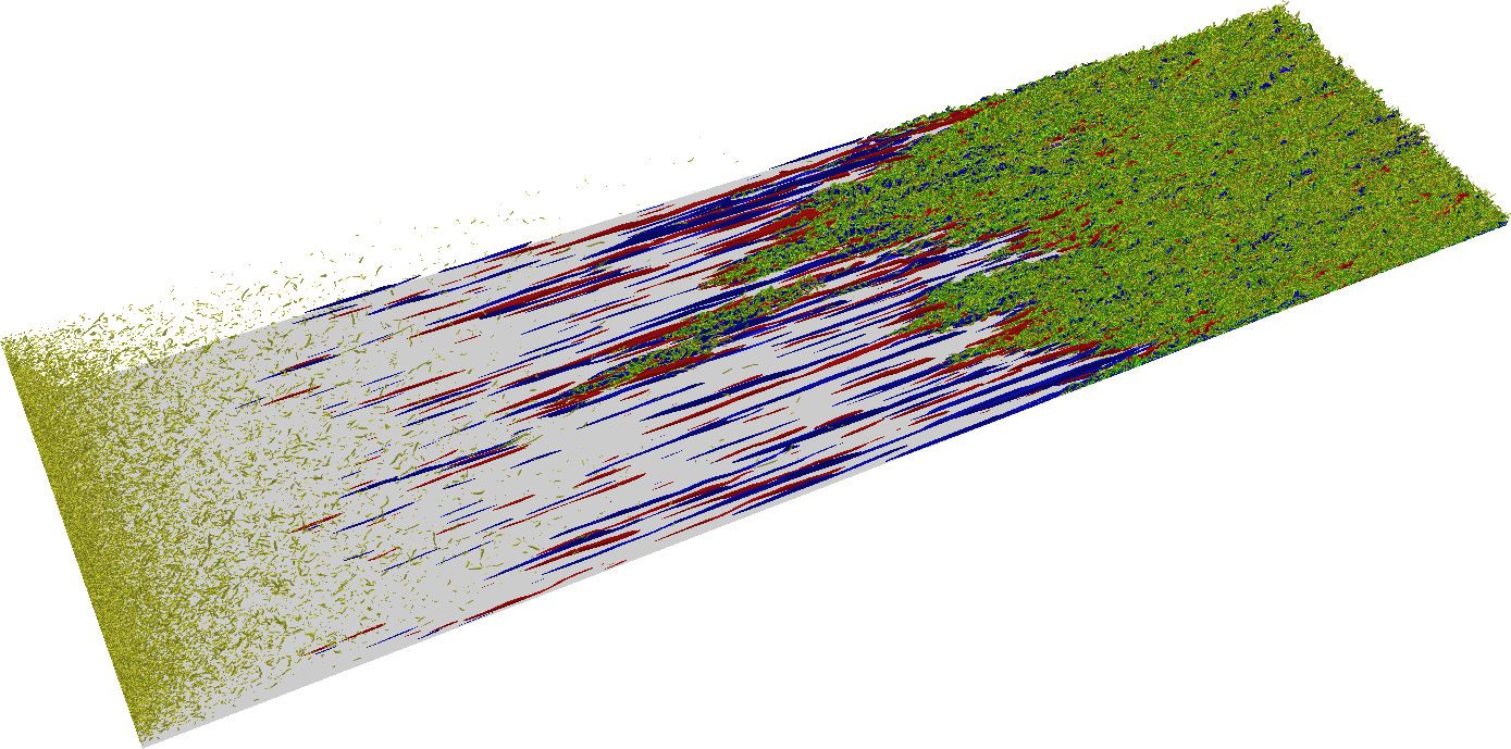
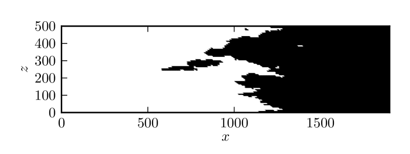
Figure 1: Two levels of representation of the turbulence transition in boundary layers. Top: a snapshot from a numerical solution of the full equations (movies are supplied with the supplemental material). Free-stream turbulence enters from the left (vortices visualized in green by isocontours of $\lambda_{2}$). As it moves along the plate, it decays and induces perturbations in the boundary layer which develop into low- and high-speed streaks (blue and red, respectively) that then break down and initiate turbulence (green regions to the right) that grow and spread to fill the boundary layer. Bottom: reduction of the above snapshot to a discrete laminar/turbulent representation according to the local spanwise wall shear. Turbulent regions are black, laminar ones white.

A snapshot from a numerical simulation in Fig. 1 (top) shows several stages of the flow development from the initial perturbations upstream through the emergence of streaks and their breakdown into isolated turbulent spots that grow to cover the entire width of the domain further downstream. The intermittency factor $\gamma$ depends on the turbulence intensity, characterized by the parameter $Tu=\sqrt{(u_{rms}^{2}+v_{rms}^{2}+w_{rms}^{2})/3}$ in units of $U_{\infty}$. We focus on the range of $Tu$ between $3\%$ and $4\%$, well inside the region $Tu\gtrsim 2\%$ where bypass transition typically occurs.

The original simulation data is transferred to a coarser Cartesian grid defining the individual cells for the model. We furthermore neglect variations in the wall-normal direction and reduce the boundary layer to two dimensions, an approach that is justified by many experimental and numerical studies. As a local indicator for turbulence the local spanwise shear stress at the wall $\tau_{z}=\partial w/\partial y|_{y=0}$ is used. Before transition to turbulence, the flow consists mainly of streamwise oriented streaks, which have high energy in the downstream velocity fluctuations but only very little in the spanwise ones. After breakdown of the streaks, the flow exhibits strong vortical motion. Strong streamwise vortices lead to a higher spanwise wall-shear stress, so that $\tau_{z}$ is high if the flow is turbulent. Furthermore, $\tau_{z}$ is a wall-based quantity, showing no ambiguity in the position where it is measured and monitored from the numerical simulations.

The grid spacing of the numerical simulations is $D_{x}=1.95$ and $D_{z}=0.65$ in units of $\delta_{0}$. For the probabilistic model, we have to determine the size of independent cells and a suitable time step. To get an estimate of an appropriate discretization, we look at the autocorrelation function of $\tau_{z}$. Since we expect the structures to be advected quickly in the downstream direction, but only slowly in the spanwise one, we calculate the purely spatial autocorrelation in the spanwise direction (Fig. 2 a) and the space-time autocorrelation in the downstream direction (Fig. 2 b).

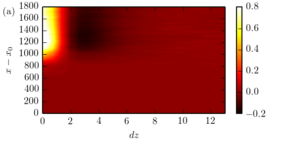
Figure 2: (a) Autocorrelation in the spanwise direction for every downstream location $x$. Before the transition region $\tau_{z}$ vanishes, afterwards the autocorrelation function is almost independent of $x$. There is a strong positive correlation for $z\lesssim 2$ and a somewhat weaker, but clear, anticorrelation for $2\lesssim z\lesssim 5$, corresponding to a vortex and the counter-rotating neighbor, respectively. (b) The autocorrelation function of $\tau_{z}$ in time and downstream direction shows a strong positive correlation in the direction $dx/dt=0.45$, indicated by the black line and corresponding to the average advection speed in the boundary layer.

The autocorrelation in the spanwise direction is computed independently for all downstream positions, $C_{z}(x,dz)=\left\langle\int\tau_{z}(x,z,t)\tau_{z}(x,z+dz,t)\mathrm{d}z\right\rangle_{t}$, with $\langle\rangle_{t}$ indicating temporal averaging. Figure 2(a) shows that it is extremely small before transition to turbulence occurs. Afterwards, it is almost independent of $x$, indicating that the size of the structures does not depend on the downstream location. There is a strong positive correlation for $z\lesssim 1.5$, corresponding to the width of a single vortex, and a somewhat weaker but still clear negative correlation for $2\lesssim z\lesssim 5$, corresponding to the counter-rotating vortex. As we want our cell size to average over one vortex pair, which ranges from $-2$ to $5$, a good estimate of $dz$ is hence given by $dz\simeq 6$-$7$ and we choose $dz=10D_{z}=6.5$ so that it is an integer multiple of the grid spacing in the numerical simulations.

Looking at the space-time autocorrelation

$$C_{xt}(dx,dt)=\left\langle\int\tau_{z}(x,z,t)\tau_{z}(x+dx,z,t+dt)\mathrm{d}x\mathrm{d}t\right\rangle_{z}$$

in Fig. 2(b), we see a very strong positive finger pointing into the plane, corresponding to the speed at which the structures are advected. The finger is rather thin, indicating that the advection speed is constant everywhere for all structures. The finger has a slope of $dx/dt=0.45$, which is depicted by the black line and we naturally choose this measure to define $dt$ once $dx$ is chosen. The autocorrelation function, however, does not give a clear estimate for $dx$ and we deliberately choose $dx=5D_{x}=9.5$ as a compromise between averaging over enough gridpoints and keeping the time step low (which means more statistics from a simulated trajectory). The time step that follows is $dt=dx/0.45=22$. We have tried different values for $dx$ during the fitting procedure outlined below and verified a posteriori that the exact choice of $dx$ does not influence our results, e.g. for the intermittency factor, as long as $dx$ is not too large. Note, however, that the turbulence spreading parameters discussed in the next section do depend on $dx$ and have to be adjusted accordingly.

The 3D box size of the simulations $L_{x}\times L_{y}\times L_{z}=2000\times 130\times 500$ translates to a 2D cell grid of size $N_{x}\times N_{z}=204\times 76$ for the model. The data is reduced to a coarser grid using local spatial averaging.

In order to distinguish between laminar and turbulent cells we choose a threshold for $\tau_{z}$ and define everything below the threshold as laminar and everything above it as turbulent. The threshold is estimated from the probability density function of $\tau_{z}$, shown in Fig. 3 for all five turbulence intensity levels. The PDF is high near $0$, drops to a minimum and then shows a peak, whose height increases with free-stream turbulence intensity as larger parts of the box are turbulent. Associating the high values near $0$ with patches of purely laminar flow and the second peak at higher values of the spanwise wall-shear stress with turbulent patches, we set the threshold in the gap separating the two at $\tau_{z}=0.3$.

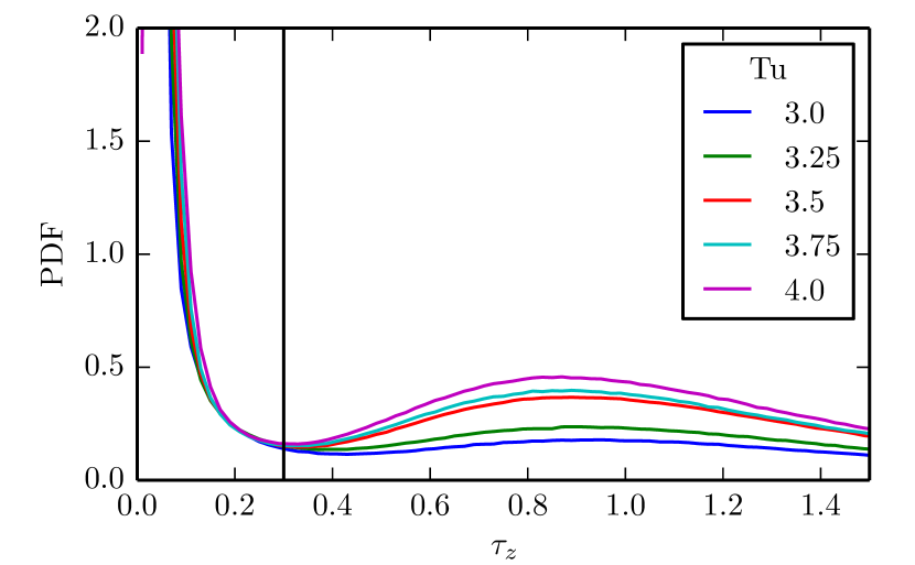
Figure 3: The probability density function of $\tau_{z}$ for different FST intensities is used to determine a threshold defining laminar and turbulent. The chosen threshold is located close to the minimum between the two peaks and is indicated by the black vertical line at $0.3$.

After applying the threshold a few undesired effects remain: we sometimes find a single laminar cell in a turbulent region or a flickering of isolated turbulent cells in a laminar region that appear for a single time step only. To prevent those spurious events from contaminating our statistics, we apply a Gaussian filter with kernel size $0.5$ cells in both spatial directions before applying the threshold.

The final result of our data processing procedure is shown in Fig. 1 (bottom), where the 2D binary representation of the above snapshot is shown. The figure suggests that our criterion captures the location of turbulent patches (green in the upper snapshot and black in the lower one) very well.

III Modelling spot evolution

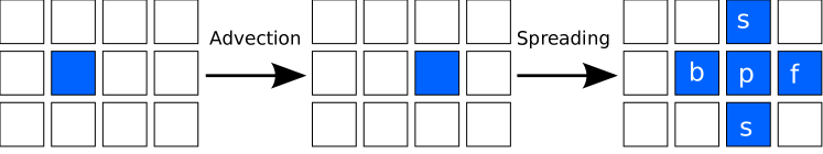
Figure 4: Reduction of the spatial and temporal dynamics on a discrete lattice of cells that are either laminar (white) or turbulent (blue). The temporal evolution of a turbulent region consists of advection by one cell to the right with persist probability $p_{p}$, and spreading to neighboring cells with probabilities $p_{b}$, $p_{s}$ and $p_{f}$.

The simulations, both in the full representation as well as in their reduced binary description, show the nucleation of turbulent spots at spatially and temporally varying positions at the upstream side, and their advection and growth in the downstream direction. We here focus on the evolution of turbulent spots, which we describe using probabilistic cellular automata (PCA) (Chaté and Manneville, 1988; Daviaud et al., 1990; Barkley, 2011; Allhoff and Eckhardt, 2012).

With the discretization of space and time discussed in section II, we now look for a discrete dynamics that updates the state of each cell. Each temporal update in the probabalistic cellular automaton follows two steps. The first deterministic step models the advection, translating all cells by one unit in the downstream direction. In a second step, the cell can spread or decay. The probabilities are $p_{f}$ to spread forward, $p_{p}$ to persist, $p_{s}$ to spread right or left and $p_{b}$ to spread backwards, as shown in Fig. 4.

The numerical values of the four probabilities are directly extracted from the numerical data in the following way: the probability that a cell $C$ is laminar after one time step, $p_{l}=p(C(x+1,z,t+1)\equiv 0)$ is given by the product of the probabilities that the surrounding cells do not spread turbulence in this cell and reads:

$$p_{l}=(1-p_{p})C(x,z,t)\cdot(1-p_{b})C(x+1,z,t)$$

$$\cdot(1-p_{f})C(x-1,z,t)\cdot(1-p_{s})C(x,z-1,t)$$

$$\cdot(1-p_{s})C(x,z+1,t)$$

Measuring $p_{l}$ for all possible configurations of surrounding cells in the numerical data, we obtain a system of equations from which the probabilities can be calculated using a least-squares algorithm.

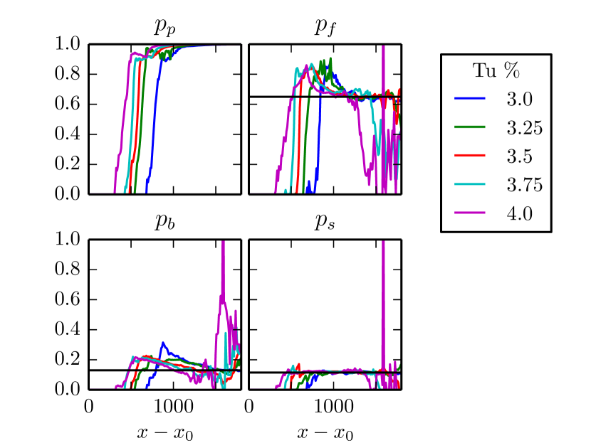
Figure 5: Probabilities to persist ($p_{p}$), spread forward ($p_{f}$), sideways ($p_{s}$) or backwards ($p_{b}$) estimated from the numerical data for different FST intensities. While there is some variation in the earliest phase of transition, where very few events happen and the statistics are poor, there is afterwards almost no variation with downstream position. Furthermore, there is no dependence of the probabilities on the level of FST disturbances – once a turbulent spot is created, its time evolution is intrinsic and independent of position and what happens in the free stream. The black lines indicate the constant values of the probabilities that are chosen for the PCA, $p_{p}$ is equal to one.

Figure 5 shows the resulting probabilities for all FST intensities. The probabilities show strong similarities for all Tu-levels, with a sharp increase near the onset of transition and a quick settling to an almost constant value afterwards, with $p_{f}$ and $p_{b}$ showing a slight overshoot near the onset. Disregarding the laminar region before any turbulence is encountered, and both onset and late stages of transition, where almost no events are detected during the simulations and the statistics is extremely poor, all probabilities appear to be almost independent of both $R$ and $Tu$. We therefore choose constant probabilities for the PCA, the values are indicated by the black lines in Fig. 5. Note that $p_{p}=1$, so that there is no significant spontaneous relaminarization inside a turbulent cell. It is worth noting that the development of turbulent spots in the transitional boundary layer can hence be described as an activated process, with the properties describing the spot evolution being independent of $R$ and $Tu$.

The probabilistic model is simulated on the cells corresponding to the coarsened grid of the numerical simulation, with $N_{x}\times N_{z}=204\times 76$ cells, spanwise periodicity and an unperturbed inflow.

IV Modelling spot nucleation

To obtain a complete description of the evolution of spots in the boundary layer, we need to supplement the spreading process with a position-dependent rate for the nucleation of new turbulent spots, $p_{c}(x)$, which enters the cellular automaton as the probability per unit time to have a nucleation event in a cell at position $x$.

The physical process underlying the nucleation of turbulent spots is the response of the boundary layer to perturbations from the free-stream turbulence. Perturbations from the FST develop streaks that grow in intensity until they break down via secondary instabilities and initiate turbulence (Andersson et al., 2001; Matsubara and Alfredsson, 2001; Brandt et al., 2004; Fransson et al., 2005; Schlatter et al., 2008; Shahinfar and Fransson, 2011). As in many experiments, in the numerical simulations that form the basis of our study the flow is continuously perturbed upstream and then advected downstream. Accordingly, the downstream development of the flow is a consequence of the time evolution of initial conditions prepared upstream. If the amplitude $A$ of an initial condition is below the threshold defined by the stable manifold of the edge state, the perturbation can be expected to decay. On the other hand, if it is sufficiently strong, it will grow exponentially fast and eventually trigger turbulence (Fig. 6). This simple nucleation model neglects spatial interactions and assumes constant energy level of the edge, which is sufficient for quantitatively accurate predictions of the location of spots and their statistical properties, as will be shown now.

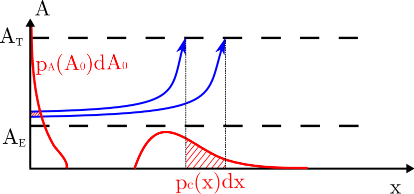
Figure 6: The basic processes underlying the transition in boundary layers: perturbations of some initial amplitude $A_{0}$ enter the boundary layer. If the initial perturbations are above the threshold $A_{E}$ associated with the stable manifold of the edge state, they exponentially grow away from the edge (blue arrows), until they reach a threshold $A_{T}$ where they trigger the creation of a turbulent spot. Since they are advected downstream while growing, we can assign a transition location to each initial amplitude. A distribution of initial amplitudes $p_{A}({A_{0}})$ hence translates into a distribution of spot nucleations $p_{c}(x)$ (red curves), allowing us to overcome the hypothesis of concentrated breakdown (Dhawan and Narasimha, 1957).

A prediction for the nucleation probabilities is obtained from the following hypotheses: (i) time and downstream location can be used interchangeably following a standard Taylor’s hypothesis; (ii) the amplitude of the initial condition $A_{0}$ has to exceed a threshold $A_{E}$ (related to the edge) in order to lead to the nucleation of any turbulence at all; (iii) since the edge is linearly unstable, the difference $A(x)-A_{E}$ will start to grow exponentially if the perturbation is larger then $A_{E}$:

$$A(x)=A_{E}+(A_{0}-A_{E})\exp(\lambda x)$$ (1)

with a Lyapunov exponent $\lambda$; (iv) turbulence is triggered once the perturbation has reached a certain amplitude $A_{T}$. Solving Eq. (1) for $A_{0}$ and substituting $A(x)=A_{T}$, we find

$$A_{0}(x)=A_{E}+(A_{T}-A_{E})\exp(-\lambda x)$$ (2)

and can then translate the distribution of initial amplitudes $p_{A}(A_{0})$ into the distribution of nucleation events $p_{c}(x)$, viz.

$$p_{c}(x)dx=p_{A}(A_{0}(x))\left|\frac{dA_{0}}{dx}\right|dx\,,$$ (3)

which leads to:

$$p_{c}(x)=p_{A}(A_{E}+(A_{T}-A_{E})\exp(-\lambda x))\times$$ (4)

$$\lambda(A_{T}-A_{E})\exp(-\lambda x)\,.$$

The initial fluctuations are assumed to be Gaussian, so that

$$p_{A}(A_{0})=\exp(-A_{0}^{2}/\sigma^{2})/(\sqrt{\pi}\sigma)\,,$$ (5)

where the standard deviation $\sigma$ increases with the turbulence level $Tu$ (Andersson et al., 2001). Then

$$p_{c}(x)=\exp\left(-\left(\frac{A_{E}+(A_{T}-A_{E})\mathrm{e}^{-\lambda x}}{\sigma}\right)^{2}-\lambda x\right)\times$$ (6)

$$\lambda(A_{T}-A_{E})/(\sqrt{\pi}\sigma)\,.$$

This expression has several parameters: (i) the standard deviation $\sigma$, (ii) the Lyapunov exponent $\lambda$, (iii) the ratio between the threshold and the edge, $r=A_{T}/A_{E}$. The parameters are fixed by fitting $\gamma$ determined from the time evolution of the cellular automaton using the modeled nucleation rate to $\gamma$ determined in the numerical simulations. The comparison shows that a good fit can be obtained with a constant $r\gg 1$, which justifies neglecting the fluctuations of the edge amplitude. The relation between $\sigma$ and $Tu$ appears to be linear. The fit also reveals a linear increase of the growth rate $\lambda$ with $Tu$. The latter is interpreted by the observation that higher $Tu$ leads to stronger streamwise vortices in the boundary layer, which give rise to a faster growth of the streaks (Fransson et al., 2005). For the final fit, we imposed functional relations and determined the parameter values indicated in Table 1. The finally obtained linear relations are $\sigma=0.226\;Tu_{\%}-0.08$ and $\lambda=(5\;Tu_{\%}-8)\cdot 10^{-3}$.

Table 1: Parameters of the nucleation model for different turbulent intensities $Tu$.

Parameter	$3.0\%$	$3.25\%$	$3.5\%$	$3.75\%$	$4.0\%$
$r$	145	145	145	145	145
$\sigma$	0.60	0.66	0.71	0.77	0.82
$\lambda\times 10^{3}$	6.79	8.05	9.32	10.6	11.8

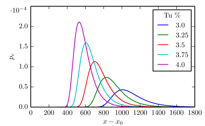
Figure 7: Nucleation rate $p_{c}(x)$ for different values of the turbulence level $Tu$. Note the upstream motion of the maximum and the narrowing of the distribution with increasing $Tu$. The position $x$ is measured in units of the displacement thickness $\delta_{0}$ at the point of entry; the offset $x_{0}$ marks the distance from the edge of the plate to the upstream end of the numerical domain.

The obtained probability distributions $p_{c}$ are shown in Fig. 7 for different values of $Tu$. One notes that they shift upstream and become narrower with increasing $Tu$. The overall shape is compatible with the data of Nolan and Zaki (2013). The rapid increase at the upstream end is a consequence of the exponential amplification and the tail on the downstream side comes from the initial conditions that are very close to the edge and that need more time to reach the turbulence level $A_{T}$.

V Results and discussion

We have developed a probabilistic cellular automaton model for the evolution of turbulent spots and a physics-inspired model for the nucleation of spots. Combining the two the full dynamics of the boundary layer can be simulated at very low computational cost.

As Fig. 8 shows, the cellular automaton model with the above nucleation rates reproduces the observed intermittency factor $\gamma$ very well. Other quantities, such as the fluctuations around the mean (Fig. 9 left column), the width of individual spots (middle column) or the number of spots (right columns) are also in very convincing agreement. We also point to a movie (available online, see the supplementary material), comparing the numerical simulations with our model, that shows very good visual agreement.

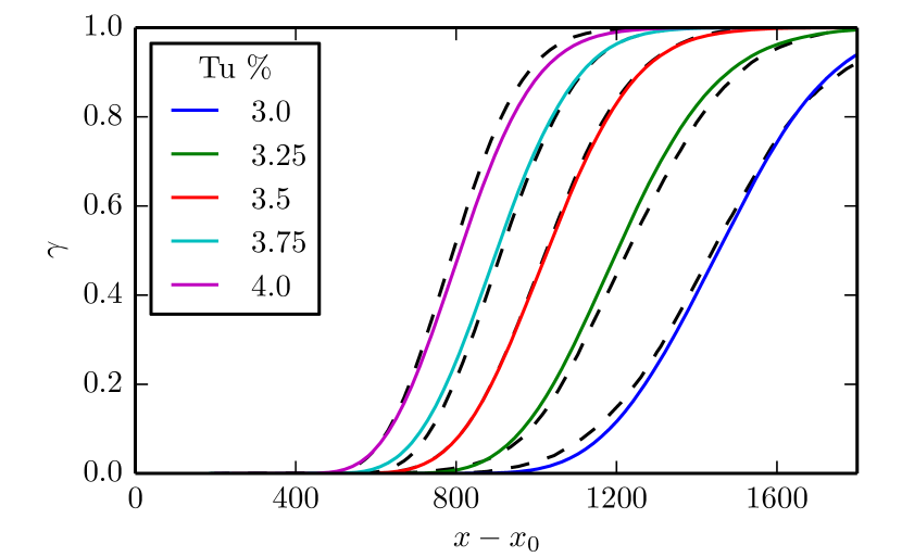
Figure 8: Comparison between the numerical simulations of the flow and the results from the cellular automaton model with intermittency curves $\gamma(x,Tu)$ for different turbulence levels. Black (dashed): simulation data, colours: automaton model.

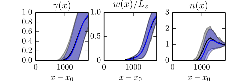
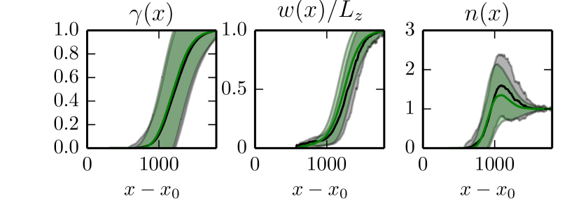
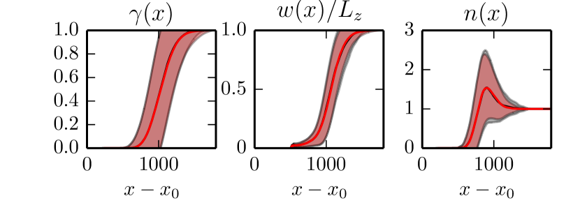
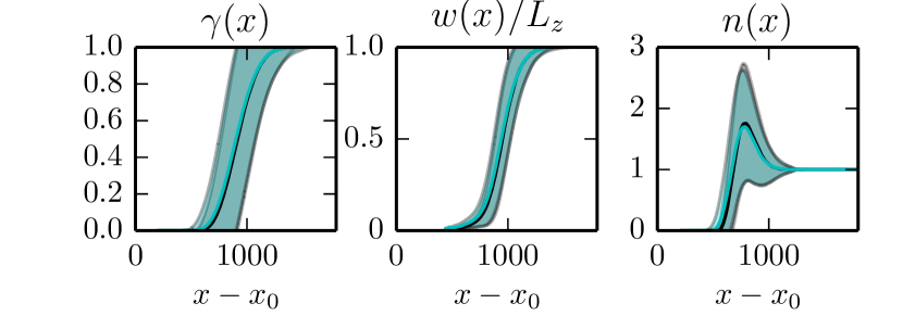
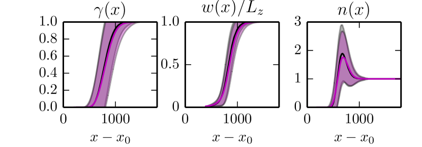
Figure 9: Detailed comparison between the numerical data and the PCA for the five values of Tu: $3.0\%$, $3.25\%$, $3.5\%$, $3.75\%$ and $4.0\%$ (from top to bottom). In addition to the intermittency factor $\gamma(x)$ (left), the average width of independent spots $w(x)$ (middle) and the number of independent spots $n(x)$ (right) is shown. For each quantity, the value from the numerical simulations of the flow is shown in black with the gray shaded area indicating $\pm$ one standard deviation and the value obtained from the cellular automaton is plotted in color. In most cases, the agreement is so good that no difference between the two curves is visible.

The results presented here show how the receptivity of the boundary layer can be combined with the nonlinear concept of a threshold curve to explain the spot nucleation mechanism. When the nucleation model is introduced into the constructed simple cellular automaton the simulation data is fully reproduced. Note that the concentrated breakdown hypothesis that assumes a fixed location for nucleation (Dhawan and Narasimha, 1957; Vinod and Govindarajan, 2004) does not reproduce the data as accurately. It is remarkable that our automaton involves only four spatially constant probabilities independent of the turbulence level. The results are an example of how the understanding that has been obtained for parallel, internal flows can be extended to the much wider class of spatially developing boundary layers.

Acknowledgements

We thank Peter Schmid for helpful comments on an earlier version of the paper and the Institute of Pure and Applied Mathematics (IPAM) at UCLA for enabling participation in the “Mathematics in Turbulence” program 2014. We acknowledge the financial support from the Alexander von Humboldt Foundation. Computer time was provided by the Swedish National Infrastructure for Computing (SNIC).

Appendix: numerical simulations

The time evolution of the boundary-layer flow is simulated using a fully spectral code Chevalier et al. (2007); Schlatter et al. (2004), which solves the incompressible Navier–Stokes equations in an open boundary-layer geometry. For the spatial discretization of the flow field a Fourier basis is used in the streamwise $x$ and spanwise $z$ directions and a Chebyshev expansion in the wall-normal $y$ one. Second-order Crank–Nicolson and third-order Runge–Kutta methods are used for time advancement of linear and nonlinear terms, respectively.

The no-slip (homogeneous Dirichlet) boundary conditions are imposed at the wall, whereas the free-stream is represented using Neumann boundary conditions. As a consequence of Fourier discretization periodic boundary conditions are imposed in the streamwise and spanwise directions. Thus in order to simulate the spatially growing boundary layer a fringe region is included at the end of the numerical domain. In the fringe region a volume forcing is added, damping all fluctuations and returning the flow to the required inflow state.

The entrance of the reference numerical domain is at a distance $x_{0}$ from the leading edge of the plate and corresponds to $R(x_{0})=300$. We measure all quantities in units of $U_{\infty}$ and $\delta_{0}^{*}$ at this location. In these units $x_{0}\approx 101$, and the Reynolds number, assuming laminar flow, is related to the distance from the leading edge $x$ by $R\approx 29.8\sqrt{x}$. We perform simulations in a box of size $L_{x}\times L_{y}\times L_{z}=2000\times 130\times 500$ with a resolution of $N_{x}\times N_{y}\times N_{z}=1024\times 201\times 768$. Since our approach is based on long-time statistics, the smallest scales of turbulence are modeled by a subgrid-scale model, which reduces the computational cost. The subgrid scales are modeled with a wall-resolved LES model of relaxation type (ADM-RT).

The free-stream turbulence at the inlet is formed by a superposition of the continuous spectrum of the Orr–Sommerfeld and Squire operators Brandt et al. (2004). The modes are chosen in the specific way in order to ensure isotropy of the resulting turbulence. An energy spectrum characteristic of isotropic homogeneous turbulence is obtained by rescaling the coefficients of the superposition. The integral length scale, which corresponds to the peak in the energy spectrum, is set to $L_{I}=10$. This value is somewhat higher than the ones used in Ref. Brandt et al. (2004) and motivates the use of a higher numerical domain in our study.

Neglecting initial transients the required simulation data is sampled over $10000$ advective time units for $Tu=3.0\%,3.25\%,3.75\%$ and $4.0\%$ and for $20000$ time units for $Tu=3.5\%$.

References

- Schlichting (2004) H. Schlichting, Boundary-layer theory (Springer, 2004).
- Schmid and Henningson (2001) P. J. Schmid and D. S. Henningson, Stability and Transition in Shear Flows, Applied mathematical sciences No. Bd. 142 (Springer, 2001).
- Emmons (1951) H. W. Emmons, J. Aeronaut. Sci. 18, 490 (1951).
- Klebanoff et al. (1962) P. S. Klebanoff, K. D. Tidstrom, and L. M. Sargent, J. Fluid Mech. 12, 1 (1962).
- Dhawan and Narasimha (1957) S. Dhawan and R. Narasimha, J. Fluid Mech. 3, 418 (1957).
- Narasimha (1985) R. Narasimha, Prog. Aerosp. Sci. 22, 29 (1985).
- Johnson and Ercan (1999) M. W. Johnson and A. H. Ercan, Int. J. Heat Fluid Flow 20, 95 (1999).
- Vinod and Govindarajan (2004) N. Vinod and R. Govindarajan, Phys. Rev. Lett. 93, 114501 (2004).
- Vinod and Govindarajan (2007) N. Vinod and R. Govindarajan, J. Turbul. 8, N2 (2007).
- Ustinov (2013) M. V. Ustinov, Fluid Dynam. 48, 192 (2013).
- Wygnanski and Champagne (1973) I. J. Wygnanski and F. H. Champagne, J. Fluid Mech. 59, 281 (1973).
- Lundbladh and Johansson (1991) A. Lundbladh and A. V. Johansson, J. Fluid Mech. 229, 499 (1991).
- Avila et al. (2011) K. Avila, D. Moxey, A. de Lozar, M. Avila, D. Barkley, and B. Hof, Science 333, 192 (2011).
- Faisst and Eckhardt (2003) H. Faisst and B. Eckhardt, Phys. Rev. Lett. 91, 224502 (2003).
- Eckhardt et al. (2007) B. Eckhardt, T. M. Schneider, B. Hof, and J. Westerweel, Annu. Rev. Fluid Mech. 39, 447 (2007).
- Eckhardt (2008) B. Eckhardt, Nonlinearity 21, T1 (2008).
- Skufca et al. (2006) J. D. Skufca, J. A. Yorke, and B. Eckhardt, Phys. Rev. Lett. 96, 174101 (2006).
- Duguet et al. (2012) Y. Duguet, P. Schlatter, D. S. Henningson, and B. Eckhardt, Phys. Rev. Lett. 108, 044501 (2012).
- Cherubini et al. (2011a) S. Cherubini, P. De Palma, J.-C. Robinet, and A. Bottaro, Phys. Fluids 23, 051705 (2011a).
- Cherubini et al. (2011b) S. Cherubini, P. De Palma, J.-C. Robinet, and A. Bottaro, J. Fluid Mech. 689, 221 (2011b).
- Duguet et al. (2013) Y. Duguet, A. Monokrousos, L. Brandt, and D. S. Henningson, Phys. Fluids 25, 084103 (2013).
- Kerswell et al. (2014) R. R. Kerswell, C. C. T. Pringle, and A. P. Willis, Rep. Prog. Phys. 77, 085901 (2014).
- Chevalier et al. (2007) M. Chevalier, P. Schlatter, A. Lundbladh, and D. S. Henningson, A pseudo-spectral solver for incompressible boundary layer flows, Tech. Rep. (KTH Mechanics, Stockholm, Sweden, 2007).
- Schlatter et al. (2004) P. Schlatter, S. Stolz, and L. Kleiser, Int. J. Heat Fluid Flow 25, 549 (2004).
- Örlü and Schlatter (2013) R. Örlü and P. Schlatter, Exp. fluids 54, 1547 (2013).
- Chaté and Manneville (1988) H. Chaté and P. Manneville, Physica D 32, 409 (1988).
- Daviaud et al. (1990) F. Daviaud, M. Bonetti, and M. Dubois, Phys. Rev. A 42, 3388 (1990).
- Barkley (2011) D. Barkley, Phys. Rev. E 84, 016309 (2011).
- Allhoff and Eckhardt (2012) K. T. Allhoff and B. Eckhardt, Fluid Dyn. Res. 44, 031201 (2012).
- Andersson et al. (2001) P. Andersson, L. Brandt, A. Bottaro, and D. S. Henningson, J. Fluid Mech. 428, 29 (2001).
- Matsubara and Alfredsson (2001) M. Matsubara and P. H. Alfredsson, J. Fluid Mech. 430, 149 (2001).
- Brandt et al. (2004) L. Brandt, P. Schlatter, and D. S. Henningson, J. Fluid Mech. 517, 167 (2004).
- Fransson et al. (2005) J. H. M. Fransson, M. Matsubara, and P. H. Alfredsson, J. Fluid Mech. 527, 1 (2005).
- Schlatter et al. (2008) P. Schlatter, L. Brandt, H. C. de Lange, and D. S. Henningson, Phys. Fluids 20, 101505 (2008).
- Shahinfar and Fransson (2011) S. Shahinfar and J. H. M. Fransson, J. Phys. Conf. Ser. 318, 043008 (2011).
- Nolan and Zaki (2013) K. P. Nolan and T. A. Zaki, J. Fluid Mech. 728, 306 (2013).