Non-Gaussian eccentricity fluctuations

Abstract

We study the fluctuations of the anisotropy of the energy density profile created in a high-energy collision at the LHC. We show that the anisotropy in harmonic $n$ has generic non-Gaussian fluctuations. We argue that these non-Gaussianities have a universal character for small systems such as p+Pb collisions, but not for large systems such as Pb+Pb collisions where they depend on the underlying non-Gaussian statistics of the initial density profile. We generalize expressions for the eccentricity cumulants $\varepsilon_{2}\{4\}$ and $\varepsilon_{3}\{4\}$ previously obtained within the independent-source model to a general fluctuating initial density profile.

I Introduction

Anisotropic flow in heavy-ion collisions Heinz:2013th can be simply understood as the hydrodynamic response to spatial anisotropy in the initial state Luzum:2013yya . The largest components of anisotropic flow are elliptic flow, $v_{2}$, and triangular flow, $v_{3}$. In hydrodynamics, both are determined to a good approximation by linear response Gardim:2014tya ; Niemi:2012aj ; Gardim:2011xv to the eccentricity $\varepsilon_{2}$ Alver:2006wh and triangularity $\varepsilon_{3}$ Alver:2010gr ; Teaney:2010vd of the initial energy density profile. As a consequence, the probability distribution of anisotropic flow Aad:2013xma directly constrains the initial geometry Renk:2014jja ; Yan:2014nsa .

The fluctuations of the initial anisotropy $\varepsilon_{n}$ are to a first approximation Gaussian Voloshin:2007pc ; Blaizot:2014nia . When the anisotropy is solely due to fluctuations (that is, with the notable exception of $v_{2}$ in non-central nucleus-nucleus collision, which is mostly driven by the eccentricity in the reaction plane), non-Gaussianities can be measured directly using higher-order cumulants of the distribution of $v_{n}$, for instance the order 4 cumulant $v_{n}\{4\}$. Non-Gaussian flow fluctuations have first been seen through $v_{3}\{4\}$ in Pb-Pb collisions ALICE:2011ab ; Chatrchyan:2013kba . Similar non-Gaussianities are seen in initial-state models of $\varepsilon_{3}$ Bhalerao:2011ry . $v_{2}\{4\}$ has also been measured in p-Pb collisions Aad:2013fja ; Chatrchyan:2013nka , and is also predicted by standard initial-state models Bozek:2013uha .

The question therefore arises as to what non-Gaussianities can tell us about the density fluctuations in the initial state: do they reveal interesting features of the dynamics, or are they the result of some general constraints? It has been pointed out for instance that the condition $|\varepsilon_{n}|\leq 1$ alone generates a universal non-Gaussian component Yan:2013laa , which matches recent measurements of higher-order cumulants $v_{2}\{6\}$ and $v_{2}\{8\}$ in p-Pb collisions Khachatryan:2015waa . On the other hand, this is known to be only approximate. General analytic results about the statistics of $\varepsilon_{n}$ can be obtained within a simple model where the initial density profile is a superposition of pointlike, independent sources Bhalerao:2006tp . Non-gaussianities arise typically as corrections to the central limit Floerchinger:2014fta . Expressions of $\varepsilon_{2}\{4\}$ Alver:2008zza and $\varepsilon_{3}\{4\}$ Bhalerao:2011bp reveal a non-trivial dependence on the initial density profile, thus breaking the universal behavior just mentioned, as will be illustrated in Sec. III.

The goal of this paper is to assess more precisely what the non-Gaussianity of anisotropy fluctuations may tell us about the initial density profile and its fluctuations, thereby extending the study initiated in Ref. Blaizot:2014wba . For simplicity, we restrict ourselves to the case of central collisions, i.e. $b=0$, where initial anisotropies are solely due to fluctuations. In the next section we recall general definitions of eccentricities and the cumulants of their probability distribution. Then in Sec. III, we review known results from the independent source model. In Sec. IV, we carry out a perturbative analysis for a general fluctuating density distribution, assuming that the fluctuations are small and uncorrelated. In Sec. V, these perturbative results are compared with full Monte Carlo simulations in order to assess the validity of the perturbative expansion. Conclusions are presented in Sec. VI. Technical material is gathered in several appendices.

II Initial anisotropies

We first recall the definitions of the anisotropy $\varepsilon_{n}$ and of the cumulants $\varepsilon_{n}\{2\}$ and $\varepsilon_{n}\{4\}$. We denote by $\rho(z)$ the energy density in a given event, where $z=x+iy$ is the complex coordinate in the transverse plane. The complex Fourier anisotropies Teaney:2010vd ; Qiu:2011iv are defined by

$$\varepsilon_{n}=\frac{\int_{z}z^{n}\rho(z)}{\int_{z}|z|^{n}\rho(z)},$$ (1)

where we use the short hand $\int_{z}=\int{\rm d}x{\rm d}y$ for the integration over the transverse plane. The definition (1) assumes that the center of the density lies at the origin. In an arbitrary coordinate system, one must replace $z$ with $z-z_{0}$, where $z_{0}=\int_{z}z\rho(z)/\int_{z}\rho(z)$ is the center of the distribution. We refer to this correction as to the “recentering” correction.

The density $\rho(z)$ fluctuates event to event, which entails fluctuations of the eccentricities $\varepsilon_{n}$. There is therefore an associated probability distribution of $|\varepsilon_{n}|$. Assuming that $v_{n}$ is proportional to $|\varepsilon_{n}|$ in every event, the probability of $|\varepsilon_{n}|$ is, up to a rescaling, the measured probability distribution of $v_{n}$ Aad:2013xma . Experimental observables involve even moments of this distribution, which are conveniently combined into cumulants. The first 2 cumulants $\varepsilon_{n}\{2\}$ and $\varepsilon_{n}\{4\}$ are defined as Borghini:2001vi ; Miller:2003kd :

$$\varepsilon_{n}\{2\}^{2} \equiv \langle|\varepsilon_{n}|^{2}\rangle$$ (2)

$$\varepsilon_{n}\{4\}^{4} \equiv 2\langle|\varepsilon_{n}|^{2}\rangle^{2}-\langle|\varepsilon_{n}|^{4}\rangle,$$ (3)

where angular brackets denote averages over events in a given centrality class.

Note that cumulants of anisotropic flow, which are defined similarly, with $\varepsilon_{n}$ replaced by $v_{n}$, were originally introduced Borghini:2001vi in order to eliminate nonflow correlations: The idea was that higher-order cumulants such as $v_{n}\{4\}$ would isolate collective motion, and that the difference between $v_{n}\{2\}$ and $v_{n}\{4\}$ was due to jets and other sources not driven by collective flow. It was then recognized that nonflow correlations are largely suppressed by rapidity gaps Adler:2003kt and that the difference between $v_{n}\{2\}$ and $v_{n}\{4\}$ mostly comes from fluctuations in the initial geometry, i.e., it originates from the difference between $\varepsilon_{n}\{2\}$ and $\varepsilon_{n}\{4\}$.

If the anisotropy is solely due to fluctuations, and if the distribution of anisotropy fluctuations is Gaussian Voloshin:2007pc , $\varepsilon_{n}\{4\}$ vanishes. Thus a non-vanishing $\varepsilon_{n}\{4\}$ directly reflects the non-Gaussianity of anisotropy fluctuations. If one assumes that $v_{n}$ is proportional to $\varepsilon_{n}$ in every event for $n=2,3$, then the observation of a positive $v_{2}\{4\}$ in proton-nucleus collisions Aad:2013fja ; Chatrchyan:2013nka implies that $\varepsilon_{2}\{4\}^{4}>0$, and the observation of a positive $v_{3}\{4\}$ ALICE:2011ab ; Chatrchyan:2013kba in nucleus-nucleus collisions, at all centralities, implies that $\varepsilon_{3}\{4\}^{4}>0$. Since the anisotropy is due to fluctuations in both cases, this in turn implies that these fluctuations are not Gaussian.

As already stated, our goal is to see what these results tell us about the fluctuations of the density $\rho(z)$. The task is complicated by the fact that the relation between density and eccentricity fluctuations is not a direct one, because the relation (1) between $\rho(z)$ and $\varepsilon_{n}$ is non linear. Also, the same relation (1) shows that $\rho(z)>0$ ensures that $|\varepsilon_{n}|\leq 1$. This puts a constraint on the allowed range of local density fluctuations. Our efforts will mostly focus on the relations between the cumulants of the density fluctuations and those of the eccentricity fluctuations. Our study is limited to $\varepsilon_{n}\{2\}$ and $\varepsilon_{n}\{4\}$, but higher-order cumulants such as $\varepsilon_{n}\{6\}$ could be studied in a similar way.

III Identical sources

We first recall known analytical results obtained within a simple model where the energy density is represented by a sum of identical, pointlike sources, much as in a Monte Carlo Glauber simulation Miller:2007ri :

$$\rho(z)=\sum_{i=1}^{N}\delta(z-z_{i}).$$ (4)

The positions $z_{i}$ of the sources, $i=1,\cdots,N$, are independent random variables with probability $p(z_{i})$ ($\int_{z}p(z)=1$) and $N\geq 2$ is fixed. With this normalization, the total energy is $\int_{z}\rho(z)=N$. It is dimensionless. Since the sources are independent, the statistics of the fluctuations of $\rho(z)$ is formally equivalent to that of the density fluctuations of a two-dimensional ideal gas of $N$ particles with an average density profile $\langle\rho(z)\rangle=Np(z)$. Inserting Eq. (4) into (1), one obtains

$$\varepsilon_{n}=\frac{\sum_{i=1}^{N}(z_{i}-z_{0})^{n}}{\sum_{i=1}^{N}|z_{i}-z_{0}|^{n}},$$ (5)

where $z_{0}=(1/N)\sum_{i=1}^{N}z_{i}$ is the center of the distribution. Throughout this paper, we assume for simplicity that $\langle\rho(z)\rangle$ has radial symmetry and depends only on $r\equiv|z|$, that is, we consider collisions at zero impact parameter. The anisotropy $\varepsilon_{n}$ still differs from zero in general because the number of sources $N$ is finite ($N$ controls the strength of the fluctuations, which vanishes as $N\to\infty$). The non linear dependence between $\rho(z)$ and $\varepsilon_{n}$ is reflected here in a non linear dependence of $\varepsilon_{n}$ on the position of the sources. This makes the analytical calculation of the distribution of $\varepsilon_{n}$ difficult for an arbitrary $p(z_{i})$.

III.1 An exact result

In the particular case where the average density profile is Gaussian, $p(z_{i})\propto\exp(-|z_{i}|^{2}/R_{0}^{2})$, the probability distribution of $|\varepsilon_{2}|$ can be calculated exactly Yan:2013laa ; Ollitrault:1992bk :

$$P(|\varepsilon_{2}|)=(N-2)|\varepsilon_{2}|\left(1-|\varepsilon_{2}|^{2}\right)^{\frac{N}{2}-2}.$$ (6)

Eqs. (2) and straightforward integrations then give the first cumulants:

$$\varepsilon_{2}\{2\} = \sqrt{\frac{2}{N}}$$ (7)

$$\varepsilon_{2}\{4\} \equiv \left(\frac{16}{N^{2}(N+2)}\right)^{1/4}.$$ (8)

In the limiting case $N=2$, the energy consists of two pointlike spots, therefore $|\varepsilon_{2}|=1$ for all events, which implies $\varepsilon_{2}\{2\}=\varepsilon_{2}\{4\}=1$.

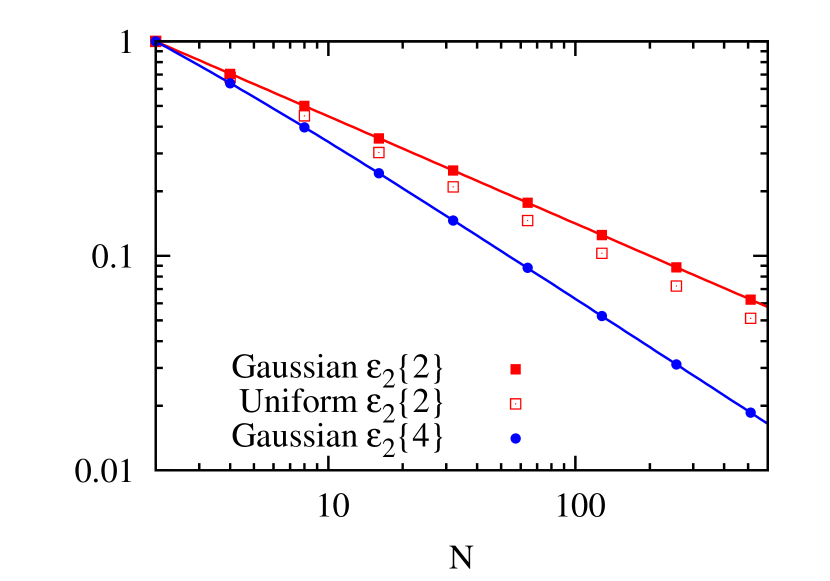
Figure 1: (Color online) Closed symbols: values of $\varepsilon_{2}\{2\}$ and $\varepsilon_{2}\{4\}$ obtained in a Monte Carlo simulation of the Gaussian independent-source model. Lines: exact result given by Eq. (7). Open squares display, for sake of comparison, the values of $\varepsilon_{2}\{2\}$ for a uniform average density profile (Sec. III.2). Statistical errors are smaller than symbols.

Both $\varepsilon_{2}\{2\}$ and $\varepsilon_{2}\{4\}$ vanish in the limit $N\to\infty$, as expected since the average density profile is isotropic. $\varepsilon_{2}\{4\}$ decreases faster than $\varepsilon_{2}\{2\}$ because eccentricity fluctuations become more and more Gaussian in the limit of large $N$. As we shall see below, the scaling laws $\varepsilon_{2}\{2\}\propto N^{-1/2}$ and $\varepsilon_{2}\{4\}\propto N^{-3/4}$ are general, in the source model, for fluctuation-dominated eccentricities in the limit $N\gg 1$ Floerchinger:2014fta .

The identical source model can easily be implemented through Monte Carlo simulations, by sampling the positions of the source $z_{i}$ according to the distribution $p(z)$, for a large number of events. Numerical results are shown in Fig. 1. They are compatible with the exact result for all $N$, as they should.

Eliminating $N$ between the two equations (7), one obtains the following relation between $\varepsilon_{2}\{2\}$ and $\varepsilon_{2}\{4\}$:

$$\varepsilon_{2}\{4\}=\varepsilon_{2}\{2\}^{3/2}\left(\frac{2}{1+\varepsilon_{2}\{2\}^{2}}\right)^{1/4}.$$ (9)

It has been conjectured Yan:2013laa that this relation, which effectively takes into account the constraint $|\varepsilon_{2}|<1$, holds to a good approximation for all models of initial conditions, and also for $\varepsilon_{3}$. However, we shall see on explicit examples that this is not always the case.

III.2 Perturbative results

More general results, i.e., valid for an arbitrary average density profile $p(z)$ and when $N\gg 1$, have been obtained for $\varepsilon_{2}$ Alver:2008zza and $\varepsilon_{3}$ Bhalerao:2011bp , by treating fluctuations as a small parameter, as we shall explain later. To leading order in $1/N$, one obtains

$$\varepsilon_{n}\{2\}^{2} = \frac{1}{N}\frac{\langle r^{2n}\rangle}{\langle r^{n}\rangle^{2}}$$ (10)

$$\varepsilon_{n}\{4\}^{4} = \frac{1}{N^{3}}\left(-\frac{8\langle r^{2n}\rangle^{3}}{\langle r^{n}\rangle^{6}}+\frac{8\langle r^{3n}\rangle\langle r^{2n}\rangle}{\langle r^{n}\rangle^{5}}\right.$$ (12)

$$-\frac{\langle r^{4n}\rangle}{\langle r^{n}\rangle^{4}}+\left.\frac{2\langle r^{2n}\rangle^{2}}{\langle r^{n}\rangle^{4}}\right),$$

where angular brackets denote average values taken with $p(z)$ (or, equivalently, the average density profile $\langle\rho(z)\rangle$), and $r\equiv|z|$.

Note that $\varepsilon_{n}\{4\}^{4}$ is the sum of two positive and two negative terms, and there are typically large cancellations. For a 2-dimensional Gaussian average density profile, for instance, $\langle r^{2k}\rangle=k!R_{0}^{2k}$ and Eq. (10) yields for $n=2$:

$$\varepsilon_{2}\{2\}^{2} = \frac{2}{N}$$ (13)

$$\varepsilon_{2}\{4\}^{4} = \frac{1}{N^{3}}\left(-64+96-24+8\right)=\frac{16}{N^{3}},$$ (14)

in agreement with the exact result (7) for $N\gg 1$.

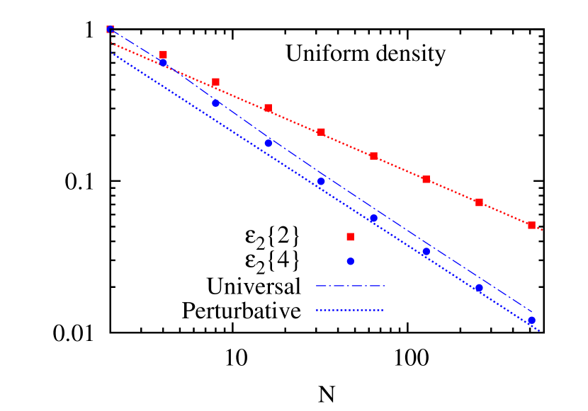
Figure 2: (Color online) Same as Fig. 1 for a uniform density distribution in a disk. Symbols are values obtained in a Monte Carlo simulation, and dotted lines are straight lines corresponding to the perturbative formulas (15). Dash-dotted line, labeled “Universal”: value of $\varepsilon_{2}\{4\}$ derived using Eq. (9), where $\varepsilon_{2}\{2\}$ in the right-hand side is taken from the Monte Carlo result.

For a generic average density profile $\langle\rho(r)\rangle$, the relative magnitudes of the four terms in the expression of $\varepsilon_{n}\{4\}^{4}$, Eq. (10), may vary. The Cauchy-Schwarz inequality $\langle xy\rangle^{2}\leq\langle x^{2}\rangle\langle y^{2}\rangle$ with $x=r^{n/2}$ and $y=r^{3n/2}$ proves that the second term is always larger than the first term (in absolute magnitude). The first term is itself at least four times larger than the fourth term. But the magnitude of the third term may vary significantly, so that the sign of $\varepsilon_{n}\{4\}^{4}$ may be negative if the density decreases slowly for large $r$. Therefore, the observation that $v_{n}\{4\}^{4}>0$ in experiments, which implies that $\varepsilon_{n}\{4\}^{4}>0$ if $v_{n}$ is proportional to $\varepsilon_{n}$ in every event, provides nontrivial information.

In order to illustrate the sensitivity of $\varepsilon_{n}$ to $\langle\rho(r)\rangle$, we carry out simulations with a uniform average density profile, $\langle\rho(r)\rangle\propto\theta(R_{0}-r)$. Figure 1 shows that $\varepsilon_{2}\{2\}$ is slightly smaller than with a Gaussian profile. This is confirmed by the analytic formulas Eq. (10): The moments are given by $\langle r^{2k}\rangle=R_{0}^{2k}/(k+1)$ and one has

$$\varepsilon_{2}\{2\}^{2} = \frac{4}{3N}$$ (15)

$$\varepsilon_{2}\{4\}^{4} = \frac{368}{135N^{3}}.$$ (16)

Comparison with Eq. (13) reveals that $\varepsilon_{2}\{2\}^{2}$ is smaller by a factor $\frac{2}{3}$. With a Gaussian density profile, it may happen that a source lies far from the center, which typically increases the anisotropy. The uniform distribution has no tail and therefore tends to produce rounder systems. Figure 2 shows that Monte Carlo results converge to the perturbative values (15) for large $N$ as expected.

The fact that the anisotropies depend on the average density profile $p(z)$ implies that the relation between $\varepsilon_{n}\{4\}$ and $\varepsilon_{n}\{2\}$ is not universal: Eq. (9) cannot always hold, as we have already indicated. Yet, as can be seen in Fig. 2, it accounts reasonably well for numerical results at all $N$, and is particularly accurate for small $N$ where it gives a much better result than the asymptotic formula (15).

In Sec. IV, the perturbative result Eq. (10) will be generalized to an arbitrary initial density profile. We shall be able to assign a physical interpretation to each of the four terms in the perturbative expansion of $\varepsilon_{n}\{4\}^{4}$, namely:

• The first term arises from the non linear relation, Eq. (1), between the eccentricity and the density $\rho(z)$. Due to this nonlinearity, even when $\rho(z)$ has a Gaussian distribution, the distribution of $\varepsilon_{n}$ can be non-Gaussian.

• The second and third term arise from the genuine non-Gaussianity of the distribution of $\rho(z)$, that is, they are related respectively to the cumulants of order three and four of the density distribution.

• The fourth term is due to energy conservation, namely, the constraint that the total energy $N$ should be exactly the same for all events.

IV Generalization to an arbitrary fluctuating density profile

We now generalize the results of Sec. III.2 to an arbitrary (typically continuous) density profile $\rho(z)$. We write $\rho(z)=\langle\rho(z)\rangle+\delta\rho(z)$, where $\langle\rho(z)\rangle$ is the density averaged over events and $\delta\rho(z)$ the fluctuation. In addition, we no longer consider the total energy $E=\int_{z}\rho(z)$ a dimensionless quantity, as in the identical source model.

IV.1 Small fluctuations

Radial symmetry implies $\int_{z}z^{n}\langle\rho(z)\rangle=0$ and Eq. (1) can be rewritten as

$$\varepsilon_{n}=\frac{\int_{z}z^{n}\delta\rho(z)}{\int_{z}r^{n}\langle\rho(z)\rangle+\int_{z}r^{n}\delta\rho(z)},$$ (17)

where we have neglected the recentering correction. We introduce the shorthand notation, for any function of $z$:

$$\delta f \equiv \frac{1}{\langle E\rangle}\int_{z}f(z)\delta\rho(z)$$ (18)

$$\langle f\rangle \equiv \frac{1}{\langle E\rangle}\int_{z}f(z)\langle\rho(z)\rangle,$$ (19)

where $\langle E\rangle$ is the average total energy:

$$\langle E\rangle=\int_{z}\langle\rho(z)\rangle.$$ (20)

With this notation, Eq. (17) can be rewritten as

$$\varepsilon_{n}=\frac{\delta z^{n}}{\langle r^{n}\rangle+\delta r^{n}}=\frac{\delta z^{n}}{\langle r^{n}\rangle}\left(1+\frac{\delta r^{n}}{\langle r^{n}\rangle}\right)^{-1}.$$ (21)

We expect $\delta z^{n}/\langle r^{n}\rangle$ and $\delta r^{n}/\langle r^{n}\rangle$ in Eq. (21) to be small for a large system and accordingly we treat them in a perturbative expansion. The size fluctuation $\delta r^{n}$ can be neglected to leading order Blaizot:2014nia , but must be taken into account at next-to-leading order, by expanding Eq. (21) in powers of $\delta r^{n}$. One thus obtains for the moments:

$$|\varepsilon_{n}|^{2} \simeq \frac{\delta z^{n}\delta\bar{z}^{n}}{\langle r^{n}\rangle^{2}}\left(1-2\frac{\delta r^{n}}{\langle r^{n}\rangle}+3\frac{(\delta r^{n})^{2}}{\langle r^{n}\rangle^{2}}+\cdots\right)$$ (22)

$$|\varepsilon_{n}|^{4} \simeq \frac{(\delta z^{n})^{2}(\delta\bar{z}^{n})^{2}}{\langle r^{n}\rangle^{4}}\left(1-4\frac{\delta r^{n}}{\langle r^{n}\rangle}+10\frac{(\delta r^{n})^{2}}{\langle r^{n}\rangle^{2}}+\cdots\right),$$

where $\bar{z}=x-iy$ denotes the complex conjugate of $z$. To perform the average over events, one is then led to evaluate averages of products of $\delta f$’s. For instance, a 2-point average is of the form:

$$\langle\delta f\,\delta g\rangle=\frac{1}{\langle E\rangle^{2}}\int_{z_{1},z_{2}}f(z_{1})g(z_{2})\langle\delta\rho(z_{1})\delta\rho(z_{2})\rangle.$$ (24)

More generally, terms of order $n$ in the fluctuations involve $n$-point functions of the density field, $\langle\delta\rho(z_{1})\cdots\delta\rho(z_{n})\rangle$. We now derive the general form of these $n$-point functions.

IV.2 Locality and cumulants

We assume that that fluctuations are correlated only over distances much shorter than any other scale of interest Blaizot:2014nia . A consequence of this locality hypothesis is that the energy $E$ contained in a transverse area $S$ much larger than the typical area $\sigma$ of a local fluctuation has almost Gaussian fluctuations. This is seen by decomposing the area $S$ in a large number $S/\sigma$ of independent subareas, and applying the central limit theorem. However, the condition $E>0$ induces non-Gaussianities that are visible when the relative fluctuations become sizable. In particular, the probability is likely to have positive skew, as illustrated in Fig. 3. Skewness is proportional to the third cumulant of the energy distribution.

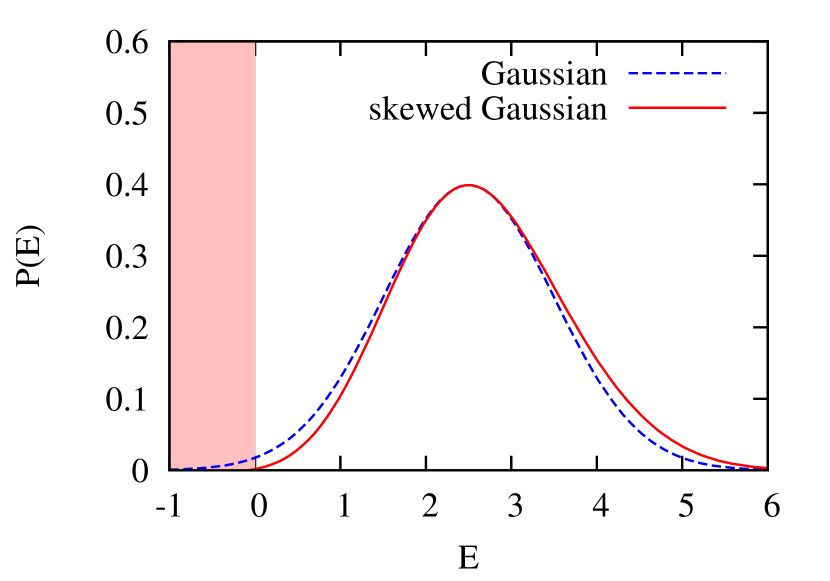
Figure 3: (Color online) Sketch of the probability of the energy $E$ in a given area. The Gaussian (dashed line) extends into the forbidden region $E<0$ (shaded area). Significant improvement is obtained by skewing the Gaussian (solid line).

Consider now two areas $S_{1}$ and $S_{2}$ large compared to $\sigma$ but small compared to the total area of the system. Let $E_{1}$ and $E_{2}$ denote the energies in these two different areas. The absence of correlations between fluctuations beyond an area of size $\sigma$ implies that $E_{1}$ and $E_{2}$ are independent variables. Denoting by $E=E_{1}+E_{2}$ the sum, one obtains for arbitrary $k$:

$$\ln\langle e^{kE}\rangle=\ln\langle e^{kE_{1}}\rangle+\ln\langle e^{kE_{2}}\rangle.$$ (25)

This function of $k$ is called the generating function of cumulants. The cumulant of order $n$, denoted by $\kappa_{n}$, is obtained by expanding to a given order $k^{n}$.

$$\ln\langle e^{kE}\rangle=\sum_{n=1}^{+\infty}\frac{k^{n}}{n!}\kappa_{n}$$ (26)

Eq. (25) shows that cumulants of the sum are sums of individual cumulants to all orders.

The additivity property Eq. (25) implies that cumulants of the energy in a cell scale like the transverse area $S$ of the cell. Therefore we denote by $\kappa_{n}(z)\equiv\kappa_{n}/S$ the density of the cumulant per unit transverse area at point $z$. At this point we note that all quantities that we are interested in are integrals of functions that are smooth on the scale of $S$. This allows us to abandon all reference to $S$ and use a completely local formalism. A general definition of $\kappa_{n}(z)$ is given in Appendix A using the formalism of functional integrals. The first cumulant $\kappa_{1}(z)$ is the average value of the energy density, $\kappa_{1}(z)=\langle\rho(z)\rangle$. The second cumulant $\kappa_{2}(z)$ is the variance. The magnitude of fluctuations is controlled by $\kappa_{2}(z)$.

The identical source model of Sec. III. does not satisfy the locality condition Eq. (25) because the total energy $N$ is fixed by construction, which introduces a long-range correlation. One recovers Eq. (25) if $N$ is allowed to fluctuate according to a Poisson distribution, as shown in Appendix C. In this case, all cumulants are equal: $\kappa_{n}(z)=\langle N\rangle p(z)$, where $\langle N\rangle$ is the average value of $N$. In the general case, one can define an effective number of sources as follows Blaizot:2014nia :

$$N_{\rm eff}\equiv\frac{(\int_{z}\kappa_{1}(z))^{2}}{\int_{z}\kappa_{2}(z)},$$ (27)

which coincides with $\langle N\rangle$ for identical sources.

Cumulants of order $3$ and higher vanish for a Gaussian distribution. The cumulants $\kappa_{3}(z)$ and $\kappa_{4}(z)$ correspond to the skewness and kurtosis, respectively.

IV.3 $n$-point functions

We show in Appendix A that the 2-point function is:

$$\langle\delta\rho(z_{1})\delta\rho(z_{2})\rangle=\kappa_{2}(z_{1})\delta(z_{1}-z_{2}),$$ (28)

where $\kappa_{2}(z)$ parametrizes the variance of the energy density at point $z$. Inserting Eq. (28) into Eq. (24), one obtains

$$\langle\delta f\,\delta g\rangle=\frac{1}{\langle E\rangle^{2}}\int_{z}f(z)g(z)\kappa_{2}(z),$$ (29)

where $\langle E\rangle=\int_{z}\kappa_{1}(z)$ (Eq. (20)). The order of magnitude of the relative fluctuation is $\langle\delta f\,\delta g\rangle/\langle f\rangle\langle g\rangle\sim 1/N_{\rm eff}$, which means that the typical order of magnitude of relative fluctuations $\delta f/\langle f\rangle$ in a given event is $1/\sqrt{N_{\rm eff}}$.

Higher-order averages are computed in a similar way, as discussed in Appendix A. In particular, the non-Gaussian character of energy fluctuations results in non-trivial $3$-point averages:

$$\langle\delta f\,\delta g\,\delta h\rangle=\frac{1}{\langle E\rangle^{3}}\int_{z}f(z)g(z)h(z)\kappa_{3}(z).$$ (30)

This quantity is of order $1/N_{\rm eff}^{2}$. In a given event, $\delta f\,\delta g\,\delta h$ is of order $1/N_{\rm eff}^{3/2}$, but after averaging over events, the result is smaller by a factor $1/\sqrt{N_{\rm eff}}$. Thus 3 and 4-point averages contribute to the same order. More generally, orders $2n-1$ and $2n$ both give contributions of order $1/N_{\rm eff}^{n}$. This implies that the expansions of $\langle|\varepsilon_{n}|^{2}\rangle$ or $\langle|\varepsilon_{n}|^{4}\rangle$ are eventually in powers of $1/N_{\rm eff}$ rather than $1/\sqrt{N_{\rm eff}}$. It also implies that the terms proportional to $\delta r^{n}$ and $(\delta r^{n})^{2}$ in Eq. (22), even though they appear to be of different orders by naive power counting, both contribute at the same (next-to-leading) order.

The fourth-order moment in Eq. (22) involves terms up to order 6 in the fluctuations. 4-point averages and higher can be reduced using Wick’s theorem (Eqs. (65) and (69)) which breaks them into a sum of products of lower-order terms and a connected part, which is much smaller and vanishes for Gaussian fluctuations.

IV.4 Perturbative results

It is now a straightforward exercise to evaluate the moments of the distribution of $|\varepsilon_{n}|$ by averaging Eq. (22) over events, keeping terms up to next-to-leading order. We introduce the following notations:

$$a \equiv \frac{\langle\delta z^{n}\,\delta\bar{z}^{n}\rangle}{\langle r^{n}\rangle^{2}}$$ (31)

$$a^{\prime} \equiv \frac{\langle(\delta r^{n})^{2}\rangle}{\langle r^{n}\rangle^{2}}$$ (32)

$$b \equiv \frac{\langle\delta z^{n}\,\delta\bar{z}^{n}\delta r^{n}\rangle}{\langle r^{n}\rangle^{3}}$$ (33)

$$c \equiv \frac{\langle(\delta z^{n})^{2}\,(\delta\bar{z}^{n})^{2}\rangle_{c}}{\langle r^{n}\rangle^{4}},$$ (34)

where the subscript $c$ in the last line denotes the connected part, defined in Appendix A by Eq. (60). We have scaled by powers of $\langle r^{n}\rangle$ so as to obtain dimensionless quantities. Then $a$, $a^{\prime}$, $b$ and $c$ are of order $1/N_{\rm eff}$, $1/N_{\rm eff}$, $1/N_{\rm eff}^{2}$ and $1/N_{\rm eff}^{3}$, respectively. Using Eqs. (29), (30) and (66), one obtains

$$a=a^{\prime} = \frac{\int_{z}r^{2n}\kappa_{2}(z)}{\left(\int_{z}r^{n}\kappa_{1}(z)\right)^{2}}$$

$$b = \frac{\int_{z}r^{3n}\kappa_{3}(z)}{\left(\int_{z}r^{n}\kappa_{1}(z)\right)^{3}}$$

$$c = \frac{\int_{z}r^{4n}\kappa_{4}(z)}{\left(\int_{z}r^{n}\kappa_{1}(z)\right)^{4}}.$$ (35)

Since one expects cumulants to be positive to all orders, these quantities are all positive. Both $b$ and $c$ result from the non-Gaussianity of density fluctuations, i.e., they are proportional to averages of the cumulants $\kappa_{3}(z)$ and $\kappa_{4}(z)$, respectively.

The moments (22) can be simply expressed in terms of these elementary building blocks using Wick’s theorem (Eqs. (65) and (69)), and using radial symmetry (which implies that $\kappa_{n}(z)$ only depends on $|z|$) to eliminate terms such as $\langle\delta z^{n}\,\delta r^{n}\rangle$ or $\langle(\delta z^{n})^{2}\rangle$:

$$\langle|\varepsilon_{n}|^{2}\rangle = a-2b+3aa^{\prime}$$ (36)

$$\langle|\varepsilon_{n}|^{4}\rangle = 2a^{2}+c-16ab+20a^{2}a^{\prime},$$ (37)

where the first term in each line is the leading order term, and the next terms are the next-to-leading corrections. The leading-order result for $\varepsilon_{n}\{2\}$ has already been obtained in Ref. Blaizot:2014nia , namely:

$$\varepsilon_{n}\{2\}^{2}\equiv\langle|\varepsilon_{n}|^{2}\rangle=a=\frac{\int_{z}r^{2n}\kappa_{2}(z)}{\left(\int_{z}r^{n}\kappa_{1}(z)\right)^{2}}.$$ (38)

Terms of order $1/N_{\rm eff}^{2}$ cancel in the 4-cumulant (2):

$$\varepsilon_{n}\{4\}^{4}=-8a^{2}a^{\prime}+8ab-c,$$ (39)

where we have kept all terms of order $1/N_{\rm eff}^{3}$, which is the leading non-trivial order for this quantity. This equation is one of the main results of this article. Together with Eq. (IV.4), it expresses the non-Gaussianity of eccentricity fluctuations in terms of the statistical properties of the underlying density field, in the regime where the perturbative expansion is valid.

We can check the result for identical, pointlike sources where $\kappa_{n}(z)=\langle N\rangle p(z)$. Eq. (IV.4) then reduces to

$$a=a^{\prime} = \frac{1}{\langle N\rangle}\frac{\langle r^{2n}\rangle}{\langle r^{n}\rangle^{2}}$$ (40)

$$b = \frac{1}{\langle N\rangle^{2}}\frac{\langle r^{3n}\rangle}{\langle r^{n}\rangle^{3}}$$ (41)

$$c = \frac{1}{\langle N\rangle^{3}}\frac{\langle r^{4n}\rangle}{\langle r^{n}\rangle^{4}}.$$ (42)

Inserting these expressions into Eq. (39), one recovers the first three terms in Eq. (10), if one replaces $N$ with $\langle N\rangle$. The missing (fourth) term is due to energy conservation (i.e., the condition that $N$ is fixed), which breaks locality. As shown in Appendix C, the missing term appears as a contribution to $c$.

We now discuss the case of a general density $\rho(x)$. If density fluctuations were Gaussian, $b$ and $c$ would vanish, which would result in $\varepsilon_{n}\{4\}^{4}<0$. The only positive contribution is the second term in Eq. (39), which originates from the third cumulant of the density fluctuations. Therefore the observation of a positive $v_{n}\{4\}$ in experiments is by itself a clear indication that the density field has positive skew.

For simplicity, we have neglected energy conservation and the recentering correction. Energy conservation is important in practice because experimental analyses are essentially done at fixed energy: Experiments use as a proxy for impact parameter an observable dubbed “centrality” which is typically based on the energy deposited in a detector (a scintillator in the case of ALICE Abelev:2013qoq ), which is strongly correlated with the total energy. Therefore one can essentially consider that the total energy $E=\int_{z}\rho(z)$ is fixed in a narrow centrality class. This imposes a constraint on the density fluctuations, which modifies the expressions of $a^{\prime}$, $b$ and $c$, as discussed in Appendix D. However, the numerical effect on eccentricity cumulants often turns out to be small, as the numerical study presented in the next section will show. As for the effect of the recentering correction, it is discussed in detail in Appendix E. It brings additional terms to Eq. (36), but these terms cancel in $\varepsilon_{n}\{4\}^{4}$ so that Eq. (39) is unchanged.

V Monte Carlo simulations

In this section we present results of numerical simulations. Our goal is twofold. First, we want to assess the domain of validity of the results obtained in Sec. IV: How large must the system be for the expansion in powers of fluctuations to be valid? Second, we want to go beyond the identical source model of Sec. III and test the perturbative results in a more general situation where cumulants of the density $\kappa_{n}(z)$ depend on the order $n$. This will be achieved by weighing the sources differently so that they are no longer identical, as discussed in Appendix B. All the Monte Carlo simulations in this section are done with a Gaussian average density profile, as in Sec. III.1.

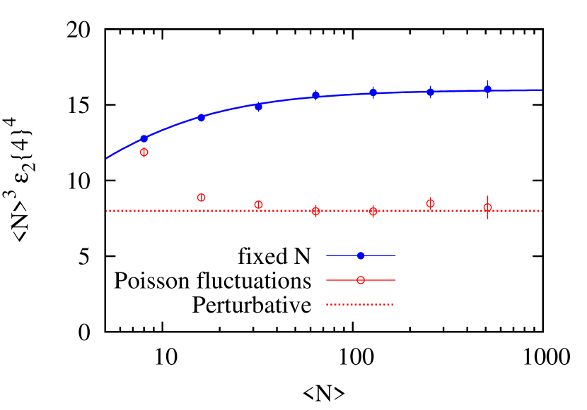
Figure 4: (Color online) $\langle N\rangle^{3}\varepsilon_{2}\{4\}^{2}$ versus $\langle N\rangle$. Closed symbols: fixed $N$, as in Fig. 1. Full line: exact result (7). Open symbols: Poisson fluctuations. Dotted line: Perturbative result Eq. (43).

V.1 Identical sources

The first set of simulations is similar to that discussed in Sec. III.1. The only difference is that the number of sources $N$ is no longer fixed but follows a Poisson distribution, so that we can apply Eq. (40). Note that the Monte Carlo simulation uses a Lagrangian specification of the density field, by sampling the position of each source, while the derivation of Sec. IV.3 use a Eulerian point of view, by specifying the correlators of the density at given points. Both Lagrangian and Eulerian descriptions are equivalent, as shown in Appendix C.

For a Gaussian density profile, Eqs. (39) and (40) give

$$\varepsilon_{n}\{4\}^{4}=\frac{8}{\langle N\rangle^{3}}.$$ (43)

Comparison with Eq. (13) shows that the lack of energy conservation decreases $\varepsilon_{n}\{4\}^{4}$ by a factor 2. One sees in Fig. 4 that Monte Carlo results quickly converge to the perturbative result (43) for large $\langle N\rangle$. The effect of energy conservation is smaller for smaller $\langle N\rangle$.

V.2 Negative binomial fluctuations

In order to test the perturbative results of Sec. IV in the more general case where cumulants differ, we allow for a simple generalization of Eq. (4), by letting the energy of each source fluctuate:

$$\rho(z)=\sum_{i=1}^{N}w_{i}\delta(z-z_{i}),$$ (44)

where $w_{i}>0$ is the energy of source $i$, and $N$ is still distributed according to a Poisson distribution to ensure locality. We assume for simplicity that the fluctuations in the position ($z_{i}$) and the strength ($w_{i}$) are uncorrelated. Then $\rho(z)$ can be viewed as the density of a polydisperse ideal gas, which generalizes the monodisperse case of Sec. III. While the cumulants of the density are all equal for identical sources, they differ in general for weighted sources: $\kappa_{n}(z)=\langle w^{n}\rangle\langle N\rangle p(z)$ (see Appendices B and C). Inserting this expression into Eq. (IV.4), one finds that weights are taken into account by replacing $r^{n}$ with $wr^{n}$ everywhere in Eqs. (40).

The fluctuations of the weights increase eccentricity fluctuations Dumitru:2012yr ; Schenke:2012fw . Thus, the effective number of sources as defined by Eq. (27) is:

$$N_{\rm eff}\equiv\frac{\langle w\rangle^{2}}{\langle w^{2}\rangle}\langle N\rangle.$$ (45)

It is smaller than $\langle N\rangle$ if $w$ fluctuates.

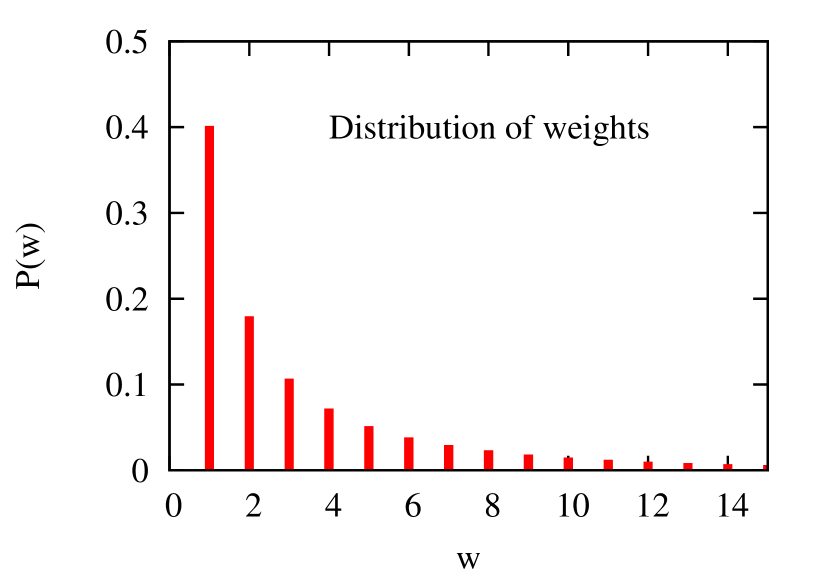
Figure 5: (Color online) Probability distribution of the energy of a single source, corresponding to Eq. (46) with $p=0.892$.

For simplicity again, we assume that $w$ is an integer, so that it represents a multiplicity rather than an energy. The probability distribution $P(w)$ used in our calculations is displayed in Fig. 5. It is chosen in such a way that the total multiplicity $\sum_{i=1}^{N}w_{i}$ follows a negative binomial distribution, in line with observations in high-energy physics experiments Giovannini:1985mz ; Gelis:2009wh . As shown in Appendix F, this is satisfied if each $w_{i}$ follows a logarithmic distribution:

$$P(w)=-\frac{1}{\ln(1-p)}\frac{p^{w}}{w}.$$ (46)

This distribution depends on a single parameter $p$, which lies between 0 and 1. The limit $p\to 0$ corresponds to identical sources, $w=1$. The larger $p$, the wider the distribution. Throughout this paper, we use the value $p=0.892$ corresponding to multiplicity fluctuations at LHC energies Kozlov:2014fqa . With this distribution, Eq. (45) gives

$$N_{\rm eff}=-\frac{p}{\ln(1-p)}\langle N\rangle.$$ (47)

With the chosen value of $p$, $N_{\rm eff}\approx 0.4\langle N\rangle$. When weights are taken into account, Eq. (40) is replaced with (121). These equations show that $N_{\rm eff}$ reflects incompletely the fluctuations of the density: in particular, for a given $N_{\rm eff}$, the non-Gaussian contractions $b$ and $c$ increase with $p$, because cumulants increase rapidly with order. Inserting Eqs. (121) into Eqs. (36) and (39), one obtains for a Gaussian density profile:

$$\varepsilon_{2}\{2\}^{2} = \frac{2}{N_{\rm eff}}-\frac{12p}{N_{\rm eff}^{2}}+{\cal O}\left(\frac{1}{N_{\rm eff}^{3}}\right)$$ (48)

$$\varepsilon_{2}\{4\}^{4} = \frac{8(1-3p^{2})}{N_{\rm eff}^{3}}+{\cal O}\left(\frac{1}{N_{\rm eff}^{4}}\right).$$ (49)

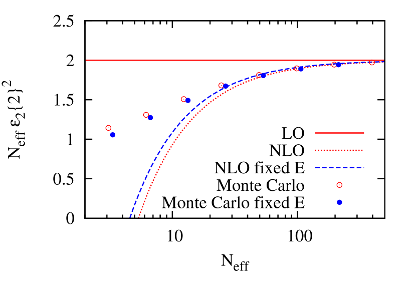
Figure 6: (Color online) $N_{\rm eff}\varepsilon_{2}\{2\}^{2}$ versus $N_{\rm eff}$. Symbols are results of Monte Carlo calculations, with (closed symbols) and without (open symbols) energy conservation. They are slightly shifted right and left, respectively, so that they do not overlap. The full line is the leading order perturbative result, the dotted and dashed lines are the next-to-leading perturbative results, with (Eq. (50)) and without (Eq. (48)) energy conservation.

Figure 6 displays Monte Carlo results for $\varepsilon_{2}\{2\}$ together with the leading order and next-to-leading order perturbative results, Eq. (48). The convergence of the numerical results to the asymptotic result is slower than for identical sources (see Figs. 2 and 4). The large magnitude of the next-to-leading order correction and the fact that it overestimates the correction are signs that the perturbative expansion diverges for small values of $N_{\rm eff}$.

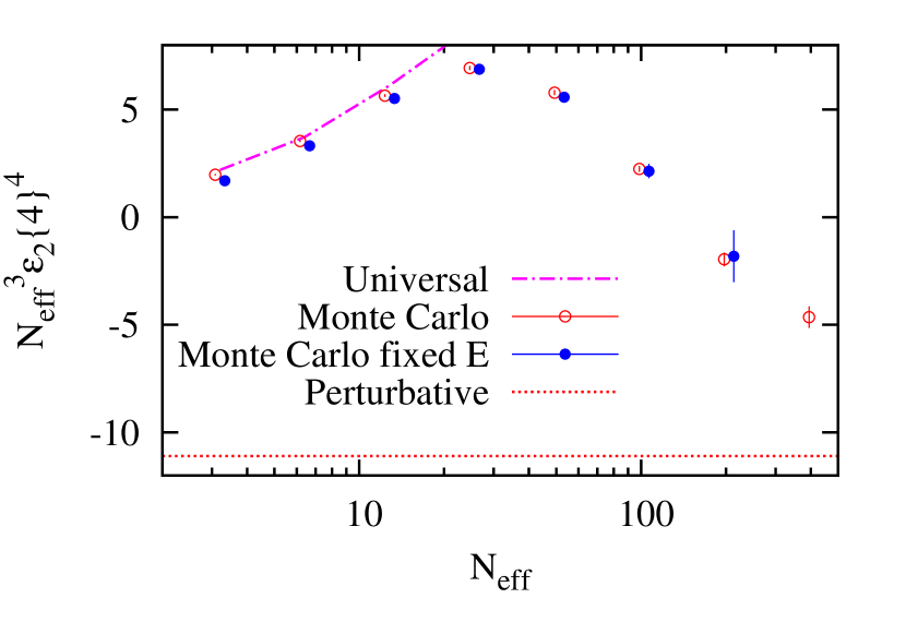
Figure 7: (Color online) $N_{\rm eff}^{3}\varepsilon_{2}\{4\}^{4}$ versus $N_{\rm eff}$. Symbols are results of Monte Carlo calculations, with (closed symbols) and without (open symbols) energy conservation. As in the previous figure, they are slightly shifted to the left or to the right. Dotted line: perturbative result (48). Dash-dotted line: Eq. (9), where $\varepsilon_{2}\{2\}$ in the right-hand side is taken from the Monte Carlo simulation.

Figure 7 displays our results for $\varepsilon_{2}\{4\}^{4}$. The perturbative result Eq. (48) is negative. On the other hand, Monte Carlo simulations return a positive $\varepsilon_{2}\{4\}^{4}$ result for $N_{\rm eff}$ up to $\sim 100$, again showing that the convergence of the perturbative expansion is very slow. For values of $N_{\rm eff}$ smaller than 20, the universal scaling, Eq. (9), gives a rather accurate result. This is not surprising, since the condition $|\varepsilon_{n}|\leq 1$ is what drives the non-Gaussianity when it is large, which occurs if $N_{\rm eff}$ is sufficiently small. As $N_{\rm eff}$ increases, agreement becomes worse as, presumably, other effects contribute to the non-Gaussianity. We do not have a satisfactory explanation of why the convergence to the asymptotic value is so slow. This observation implies that the expansion scheme chosen in Sec. IV.1 is not efficient with the additional source of fluctuations considered in this section. Our understanding is that negative binomial fluctuations increase the probability of a large fluctuation; and it is such a large, negative size fluctuation $\delta r_{n}$ in Eq. (21) which jeopardizes the power series expansion.

V.3 Energy conservation

Finally, we study the combined effect of negative binomial fluctuations and energy conservation. In the Monte Carlo simulations, this is done by generating events with arbitrary energies and keeping only those which have the exact same energy $E=\sum_{i=1}^{N}w_{i}$. This procedure is time consuming, in particular for large systems, which is the reason why our results with energy conservation, shown in Figs. 6 and 7, do not go as high in $N_{\rm eff}$ as results without energy conservation. Numerical results show that energy conservation has a very small effect for all $N_{\rm eff}$. This was not a priori expected: we have seen indeed that, for identical sources, energy conservation decreases $\varepsilon_{2}\{4\}^{4}$ by a factor 2 (see Fig. 4).

Energy conservation modifies the $n$-point functions of the density field $\rho(z)$, as shown in Appendix D. As a consequence, the values of $a^{\prime}$, $b$, $c$ are changed, and Eq. (IV.4) is replaced with (106). With logarithmic weights, energy conservation modifies Eq. (121) into Eq. (124), and the first of Eqs. (48) is replaced with

$$\varepsilon_{2}\{2\}^{2}=\frac{2}{N_{\rm eff}}-\frac{8p+2}{N_{\rm eff}^{2}}+{\cal O}\left(\frac{1}{N_{\rm eff}^{3}}\right).$$ (50)

The corresponding change is very modest, as can be seen in Fig. 6. Furthermore, it turns out that the recentering correction, discussed in Appendix E, cancels the effect of energy conservation for a Gaussian density profile, so that the full next-to-leading order expression with both energy conservation and recentering is again Eq. (48).

We have not derived the modification of $\varepsilon_{2}\{4\}^{4}$ due to energy conservation: it involves the connected 4-point function, whose modifications due to energy conservation are more complicated. However, the results displayed in Fig. 7 suggest that this modification may be of little relevance in practice.

VI Discussion

We have studied the non-Gaussianity of eccentricity fluctuation by means of Monte Carlo simulations and perturbative calculations. While all the numerical results shown in this paper are for $\varepsilon_{2}$, we have checked that conclusions also hold for the triangularity $\varepsilon_{3}$. We have generalized the perturbative calculation of Ref. Alver:2008zza to an arbitrary energy density profile, under the sole assumption that density fluctuations at different points are uncorrelated.

When a perturbative expansion, which relies of the smallness of the local density fluctuations, is valid, we have obtained evidence that the non-Gaussianity of eccentricity fluctuations largely originates from the non-Gaussianity of density fluctuations. More specifically, the skewness and kurtosis of density fluctuations give positive and negative contributions to $\varepsilon_{n}\{4\}^{4}$, respectively. While the condition that the energy is positive naturally generates such non-Gaussianities, their magnitude is not universal but depends on the higher order cumulants of the density distribution. In particular, the sign of $\varepsilon_{n}\{4\}^{4}$ is not universal, and can be negative for a large system in the presence of large (negative binomial) fluctuations of the multiplicity. Therefore, the observation that $v_{3}\{4\}^{4}$ is positive for all centralities in Pb+Pb collisions is nontrivial.

However, Monte Carlo simulations suggest that the convergence of the perturbative series can be very slow, and that results for a few hundred sources (corresponding to the number of participants in a central nucleus-nucleus collisions Blaizot:2014wba ) may vary significantly from the perturbative result. This makes it difficult to draw too definite conclusions from the present study. For small systems, on the other hand, we find that the universal statistics proposed in Ref. Yan:2013laa is generally a good approximation: More precisely, it works well for an effective number of sources smaller than 15, which is the typical number of participant nucleons for a central p+Pb collision. Our results thus confirm that this universal statistics should apply to the initial anisotropies in proton-nucleus collisions. The observation that the values of higher order cumulants of $v_{2}$ in p+Pb collisions Khachatryan:2015waa agree with predictions based on this universality therefore further supports the conclusion that elliptic flow in these systems originates from the initial eccentricity $\varepsilon_{2}$.

Appendix A Cumulants and $n$-point functions

In this Appendix we use functional methods to obtain the connected $n$-point functions and the cumulants $\kappa_{n}(z)$ introduced in Sec. IV.3. The generating functional of moments is defined as:

$${\cal Z}\left\{j(z)\right\}\equiv\left\langle\exp\left(\int_{z}j(z)\rho(z)\right)\right\rangle.$$ (51)

The $n$-point functions, such as the $2$-point function $\langle\rho(z_{1})\rho(z_{2})\rangle$, are obtained by differentiating ${\cal Z}$ twice with respect to the auxiliary source $j(z)$ and setting $j$ to 0. Connected $n$-point functions are obtained by differentiating $\ln{\cal Z}$, e.g.:

$$\langle\rho(z_{1})\rho(z_{2})\rangle_{c} = \langle\delta\rho(z_{1})\delta\rho(z_{2})\rangle$$ (52)

$$= \left.\frac{\delta^{2}\ln{\cal Z}\left\{j(z)\right\}}{\delta j(z_{1})\delta j(z_{2})}\right|_{j=0}.$$ (53)

Assuming that density fluctuations at different points are uncorrelated entails that the contributions of different points to ${\cal Z}\left\{j(z)\right\}$ factorize, therefore $\ln{\cal Z}\left\{j(z)\right\}$ can be written as an integral over $z$ of a function, which can itself be expanded in a power series

$$\ln{\cal Z}\left\{j(z)\right\}=\int_{z}\sum_{n=1}^{+\infty}\frac{j(z)^{n}}{n!}\kappa_{n}(z).$$ (54)

This equation provides a formal definition of the cumulants $\kappa_{n}(z)$. Successive differentiations of Eq. (54) with respect to $j(z)$ at $j=0$ yield connected $n$-point functions. The 2-point function is Eq. (28). The connected 3-point and 4-point functions are given by:

$$\langle\rho(z_{1})\rho(z_{2})\rho(z_{3})\rangle_{c} = \langle\delta\rho(z_{1})\delta\rho(z_{2})\delta\rho(z_{3})\rangle$$

$$= \kappa_{3}(z_{1})\delta(z_{1}-z_{2})\delta(z_{1}-z_{3}),$$

and

$$\langle\rho(1)\rho(2)\rho(3)\rho(4)\rangle_{c} \equiv \langle\delta\rho(1)\delta\rho(2)\delta\rho(3)\delta\rho(4)\rangle$$ (60)

$$-\langle\delta\rho(1)\delta\rho(2)\rangle\langle\delta\rho(3)\delta\rho(4)\rangle$$

$$-\langle\delta\rho(1)\delta\rho(3)\rangle\langle\delta\rho(2)\delta\rho(4)\rangle$$

$$-\langle\delta\rho(1)\delta\rho(4)\rangle\langle\delta\rho(2)\delta\rho(3)\rangle$$

$$= \kappa_{4}(z_{1})\delta_{12}\delta_{13}\delta_{14},$$ (61)

where $\delta\rho(i)$ stands for $\delta\rho(z_{i})$, $\delta_{12}$ for $\delta(z_{1}-z_{2})$, etc. The higher-order cumulants $\kappa_{3}(z)$ and $\kappa_{4}(z)$ express the non-Gaussian character of the initial energy density distribution.

Using Eq. (60), $4$-point averages can be decomposed as:

$$\langle\delta f\,\delta g\,\delta h\,\delta k\rangle = \langle\delta f\,\delta g\rangle\langle\delta h\,\delta k\rangle$$ (65)

$$+\langle\delta f\,\delta h\rangle\langle\delta g\,\delta k\rangle$$

$$+\langle\delta f\,\delta k\rangle\langle\delta g\,\delta h\rangle$$

$$+\langle fghk\rangle_{c},$$

where the first three terms in the right-hand side, which are given by Wick’s theorem, are of order $1/N_{\rm eff}^{2}$, while the last term is a non-Gaussian correction, of order $1/N_{\rm eff}^{3}$:

$$\langle fghk\rangle_{c}=\frac{1}{\langle E\rangle^{4}}\int_{z}f(z)g(z)h(z)k(z)\kappa_{4}(z).$$ (66)

Higher order $n$-point functions can be expanded using Wick’s theorem in a similar way. In particular, the 5-point function gets contributions from 2 and 3 point functions.

$$\langle\delta f\,\delta g\,\delta h\,\delta k\,\delta l\rangle = \langle\delta f\,\delta g\rangle\langle\delta h\,\delta k\,\delta l\rangle$$ (69)

$$+{\rm permutations}\ (10\ {\rm terms})$$

$$+\langle fghkl\rangle_{c},$$

where the various contractions are of order $1/N_{\rm eff}^{3}$, while the connected part is of order $1/N_{\rm eff}^{4}$.

Appendix B Cumulants of local sources

We derive here the expressions of the cumulants for identical, pointlike sources, starting with the case where each source has unit energy. Consider the distribution of energy $E$ in an infinitesimal transverse area $S$. This area contains a source with probability $\alpha\ll 1$. The energy $E$ in the area is $0$ with probability $1-\alpha$ and $1$ with probability $\alpha$, therefore

$$\langle e^{kE}\rangle=1-\alpha+\alpha e^{k},$$ (70)

and the generating function of cumulants is simply

$$\ln\langle e^{kE}\rangle=\alpha\left(e^{k}-1\right).$$ (71)

Using Eq. (26) and expanding to order $k^{n}$, one obtains

$$\kappa_{n}=\alpha.$$ (72)

All cumulants are equal and positive. If, in addition, locality is assumed, this result is generalized to an arbitrary area by dividing it into infinitesimal areas and using the fact that cumulants are additive.

We assume that the numbers of sources in two separate areas are independent variables. This in turn implies that the total number of sources $N$ follows a Poisson distribution.

The independent source model can be generalized by allowing the energy of each source $w$ to fluctuate with a probability $P(w)$. The previous results hold with the replacement of $e^{k}$ with $\left\langle e^{wk}\right\rangle$ in Eqs. (70) and (71), where brackets denote an average taken with respect to $P(w)$. Eq. (72) is then replaced by

$$\kappa_{n}=\alpha\left\langle w^{n}\right\rangle.$$ (73)

Cumulants are no longer equal, but still positive.

Appendix C Identical sources

We derive the connected $n$-point functions of the density for the identical source model. We insert $\rho(z)$ from Eq. (4) into the generating functional (51):

$${\cal Z}\left\{j(z)\right\} = \left\langle\prod_{i=1}^{N}\exp\left(j(z_{i})\right)\right\rangle$$ (74)

$$= \sum_{N=0}^{+\infty}p_{N}\left(\int_{z}p(z)e^{j(z)}\right)^{N},$$ (75)

where $p_{N}$ is the probability of having $N$ sources and $p(z)$ is the probability distribution of a source in the transverse plane. We now study two versions of the independent source model: the case where $N$ follows a Poisson distribution, and the case where $N$ is fixed.

If $N$ follows a Poisson distribution, then $p_{N}=e^{-\langle N\rangle}\langle N\rangle^{N}/N!$. By resumming the series in Eq. (74), one obtains

$$\ln{\cal Z}\left\{j(z)\right\}=\langle N\rangle\left(\int_{z}p(z)e^{j(z)}-1\right).$$ (76)

This equation is of the type (54) with $\kappa_{n}(z)=\langle N\rangle p(z)$. Connected $n$-point functions are therefore local, and cumulants $\kappa_{n}(z)$ are all equal, as expected from the discussion of Appendix B.

For fixed $N$, Eq. (74) yields

$$\ln{\cal Z}\left\{j(z)\right\}\equiv N\ln\left(\int_{z}p(z)e^{j(z)}\right).$$ (77)

Thus the connected $n$-point functions to all orders are proportional to $N$. Successive differentiations with respect to $j$ at $j=0$ give:

$$\langle\rho(z)\rangle=Np(z)$$ (78)

and, using Eq. (52):

$$\langle\delta\rho(z_{1})\delta\rho(z_{2})\rangle=N\left(p(z_{1})\delta(z_{1}-z_{2})-p(z_{1})p(z_{2})\right).$$ (79)

The first term in the right-hand side of Eq. (79) is a local correlation. The second term is a disconnected term: this term results from the constraint $\sum_{z}\delta\rho(z)=0$: the integral over $z$ of Eq. (79) is $0$.

The connected 3-point and 4-point functions are

$$\langle\delta\rho(z_{1})\delta\rho(z_{2})\delta\rho(z_{3})\rangle = Np(z_{1})\delta(z_{1}-z_{2})\delta(z_{1}-z_{3})$$ (84)

$$-Np(z_{1})p(z_{2})\delta(z_{2}-z_{3})$$

$$-Np(z_{2})p(z_{3})\delta(z_{3}-z_{1})$$

$$-Np(z_{3})p(z_{1})\delta(z_{1}-z_{2})$$

$$+2Np(z_{1})p(z_{2})p(z_{3}).$$

and

$$\langle\rho(1)\rho(2)\rho(3)\rho(4)\rangle_{c} = Np(1)\delta_{12}\delta_{13}\delta_{14}$$ (89)

$$-N\left(p(1)\delta_{12}\delta_{13}p(4)+...\right)$$

$$-N\left(p(1)\delta_{12}p(3)\delta_{34}+...\right)$$

$$+2N\left(p(1)\delta_{12}p(3)p(4)+...\right)$$

$$-6Np(1)p(2)p(3)p(4),$$

where $\delta\rho(i)$ stands for $\delta\rho(z_{i})$, where $\delta_{12}$ stands for $\delta(z_{1}-z_{2})$, etc., and where $+...$ means that one should average over all permutations, which yield 4, 3 and 6 terms respectively for the 2nd, 3rd and 4th lines of Eq. (89). The integral over $z_{1}$ is zero because of energy conservation.

After inserting Eqs. (79), (84) and (89) into the definitions of $a$, $a^{\prime}$, $b$ and $c$, Eq. (31), one finds that the condition that $N$ is fixed modifies Eq. (40) into

$$a = \frac{1}{\langle N\rangle}\frac{\langle r^{2n}\rangle}{\langle r^{n}\rangle^{2}}$$ (90)

$$a^{\prime} = \frac{1}{\langle N\rangle}\left(\frac{\langle r^{2n}\rangle}{\langle r^{n}\rangle^{2}}-1\right)$$ (91)

$$b = \frac{1}{\langle N\rangle^{2}}\left(\frac{\langle r^{3n}\rangle}{\langle r^{n}\rangle^{3}}-\frac{\langle r^{2n}\rangle}{\langle r^{n}\rangle^{2}}\right)$$ (92)

$$c = \frac{1}{\langle N\rangle^{3}}\left(\frac{\langle r^{4n}\rangle-2\langle r^{2n}\rangle^{2}}{\langle r^{n}\rangle^{4}}\right).$$ (93)

The first coefficient $a$ is unchanged. The modifications of $a^{\prime}$ and $b$ cancel in the combination $-aa^{\prime}+b$ entering the expression of $\varepsilon_{n}\{4\}$, Eq. (39). The modification of $c$, which produces the last term in Eq. (10), is due to the 3rd line of Eq. (89).

Appendix D Energy conservation

We now derive the expressions of connected $n$-point functions for an arbitrary density profile $\rho(z)$ when the total energy is fixed. Similar results have been obtained for momentum conservation Borghini:2000cm ; Borghini:2003ur . We denote by ${\cal Z}_{E}\left\{j(z)\right\}$ the generating function corresponding to a fixed energy $E$:

$${\cal Z}_{E}\left\{j(z)\right\}\equiv\frac{\left\langle\exp\left(\int_{z}j(z)\rho(z)\right)\delta\left(E-\int_{z}\rho(z)\right)\right\rangle}{\left\langle\delta\left(E-\int_{z}\rho(z)\right)\right\rangle}.$$ (94)

It is normalized so that ${\cal Z}_{E}\left\{j=0\right\}=1$. Using the integral representation of the Dirac distribution, $\delta(x)=\frac{1}{2\pi}\int e^{-ikx}dk$, one can express ${\cal Z}_{E}$ in terms of ${\cal Z}$ using Eq. (51):

$${\cal Z}_{E}\left\{j(z)\right\}=\frac{\int_{-\infty}^{+\infty}\exp\left(-ikE\right){\cal Z}\{j(z)+ik\}dk}{\int_{-\infty}^{+\infty}\exp\left(-ikE\right){\cal Z}\{ik\}dk}.$$ (95)

The integral over $k$ in the numerator is evaluated using the saddle point method. The saddle point $k_{0}$ is obtained by truncating the cumulant expansion Eq. (54) to order 2, inserting it into (95), and differentiating the exponent with respect to $k$:

$$ik_{0}=\frac{E-\int_{z}\kappa_{1}(z)-\int_{z}j(z)\kappa_{2}(z)}{\int_{z}\kappa_{2}(z)}.$$ (96)

In the saddle point approximation, the integral in the numerator of Eq. (95) is obtained by evaluating the integrand at $k=k_{0}$. One thus obtains

$$\ln{\cal Z}_{E}\left\{j(z)\right\} = -ik_{0}E+\int_{z}(j(z)+ik_{0})\kappa_{1}(z)$$ (98)

$$+\frac{1}{2}\int_{z}(j(z)+ik_{0})^{2}\kappa_{2}(z),$$

where we have left out the contribution of the denominator which is independent of $j$. The connected $n$-point functions are then obtained by differentiating $\ln{\cal Z}_{E}\left\{j(z)\right\}$ at $j=0$. The one-point function is the average value of the density:

$$\langle\rho(z_{1})\rangle=\kappa_{1}(z_{1})+\frac{E-\int_{z}\kappa_{1}(z)}{\int_{z}\kappa_{2}(z)}\kappa_{2}(z_{1}).$$ (99)

The first term in the right-hand side of Eq. (99) is the average value of $\rho(z)$ in the absence of energy conservation, while the second term is the correction due to energy conservation. This equation means that the energy excess $E-\int_{z}\kappa_{1}(z)$ is distributed in the transverse plane proportionally to the variance $\kappa_{2}(z)$.

The 2-point function (28) becomes:

$$\langle\delta\rho(z_{1})\delta\rho(z_{2})\rangle=\kappa_{2}(z_{1})\delta(z_{1}-z_{2})-\frac{\kappa_{2}(z_{1})\kappa_{2}(z_{2})}{\int_{z}\kappa_{2}(z)}.$$ (100)

Note that it does not involve the value of $E$. One can check that the right-hand side vanishes upon integration over $z_{1}$, as expected from the condition of energy conservation which implies $\int_{z}\delta\rho(z)=0$.

The connected $3$-point function is obtained by expanding the generating functional ${\cal Z}_{E}$ to first order in the higher-order cumulants $\kappa_{3}$. The only effect of energy conservation is to replace $j(z)$ by $j(z)+ik_{0}$, or (since the constant term drops upon differentiation) through the substitution

$$j(z)\rightarrow j(z)-\frac{\int_{z^{\prime}}j(z^{\prime})\kappa_{2}(z^{\prime})}{\int_{z^{\prime}}\kappa_{2}(z^{\prime})}.$$ (101)

Eq. (A) becomes:

$$\langle\delta\rho(z_{1})\delta\rho(z_{2})\delta\rho(z_{3})\rangle = \kappa_{3}(z_{1})\delta(z_{1}-z_{2})\delta(z_{1}-z_{3})$$ (105)

$$-\frac{\kappa_{3}(z_{1})\delta(z_{1}-z_{2})\kappa_{2}(z_{3})+{\rm perm.}}{\int_{z}\kappa_{2}(z)}$$

$$+\frac{\kappa_{3}(z_{1})\kappa_{2}(z_{2})\kappa_{2}(z_{3})+{\rm perm.}}{\left(\int_{z}\kappa_{2}(z)\right)^{2}}$$

$$-\frac{\int\kappa_{3}}{\left(\int\kappa_{2}\right)^{3}}\kappa_{2}(z_{1})\kappa_{2}(z_{2})\kappa_{2}(z_{3})$$

The second and third lines must be summed over circular permutations of $z_{1},z_{2},z_{3}$. One may again check that the right-hand side vanishes upon integration over $z_{1}$. Note that the three-point function involves cumulants of two different orders $\kappa_{2}$ and $\kappa_{3}$, and that it is linear in $\kappa_{3}$. This linearity is due to the fact that we evaluate the non-Gaussanity to first (linear) order. In the case of identical sources, where $\kappa_{3}(z)=\kappa_{2}(z)$, one recovers Eq. (84). Note that the 2-point function and 3-point functions do not involve $E$. The correlations are not changed by triggering on the tail of the distribution, that is, on ultracentral collisions.

Energy conservation modifies Eqs. (31) to

$$a = \frac{\int_{z}r^{2n}\kappa_{2}(z)}{\left(\int_{z}r^{n}\kappa_{1}(z)\right)^{2}}$$ (106)

$$a^{\prime} = \frac{\int_{z}r^{2n}\kappa_{2}(z)}{\left(\int_{z}r^{n}\kappa_{1}(z)\right)^{2}}-\frac{\left(\int_{z}r^{n}\kappa_{2}(z)\right)^{2}}{\left(\int_{z}r^{n}\kappa_{1}(z)\right)^{2}\int_{z}\kappa_{2}(z)}$$ (107)

$$b = \frac{\int_{z}r^{3n}\kappa_{3}(z)}{\left(\int_{z}r^{n}\kappa_{1}(z)\right)^{3}}-\frac{\int_{z}r^{2n}\kappa_{3}(z)\int_{z}r^{n}\kappa_{2}(z)}{\left(\int_{z}r^{n}\kappa_{1}(z)\right)^{3}\int_{z}\kappa_{2}(z)},$$ (108)

Note that the expression of $a$ is unchanged, so that the leading order anisotropy (38) is not affected by energy conservation. For identical sources, where $\kappa_{n}(z)$ is independent of the order $n$, Eq. (106) reduces to Eq. (90). We have not derived the modified expression of $c$, which involves the connected 4-point function.

Appendix E Recentering correction

We discuss here the effect of the recentering correction on perturbative results. Our discussion is limited to $\varepsilon_{2}$ for simplicity. The recentering correction arises from the requirement that the coordinate system be centered in every event. When one takes it into account, Eq. (21) is replaced by Bhalerao:2011bp

$$\varepsilon_{2}=\frac{\delta z^{2}-(\delta z)^{2}}{\langle r^{2}\rangle}\left(1+\frac{\delta r^{2}}{\langle r^{2}\rangle}-\frac{\delta z\,\delta\bar{z}}{\langle r^{2}\rangle}\right)^{-1}.$$ (109)

In order to evaluate the moment $\langle|\varepsilon_{2}|^{2}\rangle$ to next-to-leading order in the fluctuations, as in Sec. IV.4, we must keep all terms of order 3 and 4 in the fluctuations. The recentering correction introduces new nontrivial contractions, in addition to those defined in Eq. (31):

$$d \equiv \frac{\langle(\delta z)^{2}(\delta\bar{z})^{2}\rangle}{\langle r^{2}\rangle^{2}}=\frac{2\left(\int_{z}r^{2}\kappa_{2}(z)\right)^{2}}{\langle E\rangle^{2}\left(\int_{z}r^{2}\kappa_{1}(z)\right)^{2}}$$ (110)

$$e \equiv \frac{\langle\delta z^{2}\delta\bar{z}^{2}\delta z\delta\bar{z}\rangle}{\langle r^{2}\rangle^{3}}=\frac{\int_{z}r^{4}\kappa_{2}(z)\int_{z}r^{2}\kappa_{2}(z)}{\langle E\rangle\left(\int_{z}r^{2}\kappa_{1}(z)\right)^{3}}$$ (111)

$$f \equiv \frac{\langle\delta z^{2}(\delta\bar{z})^{2}\rangle}{\langle r^{2}\rangle^{2}}=\frac{\int_{z}r^{4}\kappa_{3}(z)}{\langle E\rangle\left(\int_{z}r^{2}\kappa_{1}(z)\right)^{2}},$$ (112)

which are all of order $1/N_{\rm eff}^{2}$ according to the power counting of Sec. IV.3. The first of Eqs. (36) becomes

$$\langle|\varepsilon_{2}|^{2}\rangle=a-2b+3aa^{\prime}+d+2e-2f.$$ (113)

Let us check the validity of these additional terms in the particular case of identical sources. For identical sources, all cumulants are equal and the energy $E$ is just the number of sources $N$, therefore $e=f$ and $d=2/\langle N\rangle^{2}$. For a Gaussian density profile, the exact results are $\langle|\varepsilon_{2}|^{2}\rangle=2/N$ with recentering and $\langle|\varepsilon_{2}|^{2}\rangle=2/(N+1)$ without recentering. The recentering correction is therefore $2/N-2/(N+1)\simeq 2/N^{2}$, in agreement with our perturbative estimate for large $N$.

We have checked that the recentering correction does not affect the result (39), i.e., it does contribute to $\varepsilon_{2}\{4\}^{4}$ to order $1/N^{3}$.

Appendix F Logarithmic weights

In this section, we explain how to choose the weights, in an independent-source model, in such a way that the distribution of the total energy is a negative binomial. The negative binomial distribution is

$$P_{NBD}(w)=\begin{pmatrix}w+k-1\cr w\end{pmatrix}p^{w}(1-p)^{k},$$ (114)

where $p$ and $k$ are two parameters, with $0\leq p<1$ and $k>0$. If two variables $w_{1}$ and $w_{2}$ are both distributed according to $P_{NBD}(w)$, then the sum $w_{1}+w_{2}$ also follows a negative binomial distribution with the same $p$ and $k\to 2k$. Thus $p$ is an intensive quantity and $k$ an extensive quantity. In limit of a small area, defined by $k\to 0$, Eq. (114) reduces to

$$P_{NBD}(0) = 1+k\ln(1-p)$$ (115)

$$P_{NBD}(w) = k\frac{p^{w}}{w}\ {\rm for}\ w\geq 1.$$ (116)

The probability of finding a source within the small area is defined as

$$\alpha\equiv 1-P_{NBD}(0)=\sum_{w=1}^{+\infty}P_{NBD}(w)=-k\ln(1-p).$$ (117)

This equation gives $k$ as a function of $\alpha$. Inserting into the second line of Eq. (115), One obtains $P_{NBD}(w)=\alpha P(w)$ for $w\geq 1$, where $P(w)$ is the distribution of $w$ for a single source, given by Eq. (46).

The moments of the distribution $P(w)$ can be calculated analytically. One obtains

$$\frac{\langle w^{2}\rangle}{\langle w\rangle^{2}} = \frac{-\ln(1-p)}{p}$$ (118)

$$\frac{\langle w^{3}\rangle}{\langle w\rangle^{3}} = \left(\frac{-\ln(1-p)}{p}\right)^{2}(1+p)$$ (119)

$$\frac{\langle w^{4}\rangle}{\langle w\rangle^{4}} = \left(\frac{-\ln(1-p)}{p}\right)^{3}(1+4p+p^{2}).$$ (120)

The cumulants of the energy density are proportional to the moments of $w$ as shown in Appendix B: $\kappa_{n}(z)=\langle N\rangle\langle w^{n}\rangle p(z)$. Inserting the above expressions into Eq. (IV.4), one obtains

$$a=a^{\prime} = \frac{1}{N_{\rm eff}}\frac{\langle r^{2n}\rangle}{\langle r^{n}\rangle^{2}}$$ (121)

$$b = \frac{(1+p)}{N_{\rm eff}^{2}}\frac{\langle r^{3n}\rangle}{\langle r^{n}\rangle^{3}}$$ (122)

$$c = \frac{(1+4p+p^{2})}{N_{\rm eff}^{3}}\frac{\langle r^{4n}\rangle}{\langle r^{n}\rangle^{4}},$$ (123)

where $N_{\rm eff}$ is defined by Eq. (47). Eqs. (121) reduces to Eqs. (40) in the limit $p\to 0$, as expected. Inserting Eq. (121) into Eqs. (36) and (39), one obtains Eq. (48).

With energy conservation taken into account, one uses Eq. (106) instead of Eq. (IV.4):

$$a = \frac{1}{N_{\rm eff}}\frac{\langle r^{2n}\rangle}{\langle r^{n}\rangle^{2}}$$ (124)

$$a^{\prime} = \frac{1}{N_{\rm eff}}\left(\frac{\langle r^{2n}\rangle}{\langle r^{n}\rangle^{2}}-1\right)$$ (125)

$$b = \frac{(1+p)}{N_{\rm eff}^{2}}\left(\frac{\langle r^{3n}\rangle}{\langle r^{n}\rangle^{3}}-\frac{\langle r^{2n}\rangle}{\langle r^{n}\rangle^{2}}\right).$$ (126)

We finally consider the effect of the recentering correction. With logarithmic weights, Eqs. (110) become

$$d = \frac{2}{N_{\rm eff}^{2}}$$ (127)

$$e = \frac{1}{N_{\rm eff}^{2}}\frac{\langle r^{4}\rangle}{\langle r^{2}\rangle^{2}}$$ (128)

$$f = \frac{1+p}{N_{\rm eff}^{2}}\frac{\langle r^{4}\rangle}{\langle r^{2}\rangle^{2}}.$$ (129)

Inserting Eqs. (127) and (124) into Eqs. (113), one finds that the contribution to $\varepsilon_{2}\{2\}^{2}$ from recentering exactly cancels the contribution from energy conservation for a Gaussian density profile.

References

- (1) U. Heinz and R. Snellings, Ann. Rev. Nucl. Part. Sci. 63, 123 (2013) [arXiv:1301.2826 [nucl-th]].
- (2) M. Luzum and H. Petersen, J. Phys. G 41, 063102 (2014) [arXiv:1312.5503 [nucl-th]].
- (3) F. G. Gardim, J. Noronha-Hostler, M. Luzum and F. Grassi, Phys. Rev. C 91, no. 3, 034902 (2015) [arXiv:1411.2574 [nucl-th]].
- (4) H. Niemi, G. S. Denicol, H. Holopainen and P. Huovinen, Phys. Rev. C 87, no. 5, 054901 (2013) [arXiv:1212.1008 [nucl-th]].
- (5) F. G. Gardim, F. Grassi, M. Luzum and J. Y. Ollitrault, Phys. Rev. C 85, 024908 (2012) [arXiv:1111.6538 [nucl-th]].
- (6) B. Alver et al. [PHOBOS Collaboration], Phys. Rev. Lett. 98, 242302 (2007) [nucl-ex/0610037].
- (7) B. Alver and G. Roland, Phys. Rev. C 81, 054905 (2010) Erratum: [Phys. Rev. C 82, 039903 (2010)] [arXiv:1003.0194 [nucl-th]].
- (8) D. Teaney and L. Yan, Phys. Rev. C 83, 064904 (2011) [arXiv:1010.1876 [nucl-th]].
- (9) G. Aad et al. [ATLAS Collaboration], JHEP 1311, 183 (2013) [arXiv:1305.2942 [hep-ex]].
- (10) T. Renk and H. Niemi, Phys. Rev. C 89, no. 6, 064907 (2014) [arXiv:1401.2069 [nucl-th]].
- (11) L. Yan, J. Y. Ollitrault and A. M. Poskanzer, Phys. Lett. B 742, 290 (2015) [arXiv:1408.0921 [nucl-th]].
- (12) S. A. Voloshin, A. M. Poskanzer, A. Tang and G. Wang, Phys. Lett. B 659, 537 (2008) [arXiv:0708.0800 [nucl-th]].
- (13) J. P. Blaizot, W. Broniowski and J. Y. Ollitrault, Phys. Lett. B 738, 166 (2014) [arXiv:1405.3572 [nucl-th]].
- (14) K. Aamodt et al. [ALICE Collaboration], Phys. Rev. Lett. 107, 032301 (2011) [arXiv:1105.3865 [nucl-ex]].
- (15) S. Chatrchyan et al. [CMS Collaboration], Phys. Rev. C 89, no. 4, 044906 (2014) [arXiv:1310.8651 [nucl-ex]].
- (16) R. S. Bhalerao, M. Luzum and J. Y. Ollitrault, J. Phys. G 38, 124055 (2011) [arXiv:1106.4940 [nucl-ex]].
- (17) G. Aad et al. [ATLAS Collaboration], Phys. Lett. B 725, 60 (2013) [arXiv:1303.2084 [hep-ex]].
- (18) S. Chatrchyan et al. [CMS Collaboration], Phys. Lett. B 724, 213 (2013) [arXiv:1305.0609 [nucl-ex]].
- (19) P. Bozek and W. Broniowski, Phys. Rev. C 88, no. 1, 014903 (2013) [arXiv:1304.3044 [nucl-th]].
- (20) L. Yan and J. Y. Ollitrault, Phys. Rev. Lett. 112, 082301 (2014) [arXiv:1312.6555 [nucl-th]].
- (21) V. Khachatryan et al. [CMS Collaboration], Phys. Rev. Lett. 115, no. 1, 012301 (2015) [arXiv:1502.05382 [nucl-ex]].
- (22) R. S. Bhalerao and J. Y. Ollitrault, Phys. Lett. B 641, 260 (2006) [nucl-th/0607009].
- (23) S. Floerchinger and U. A. Wiedemann, JHEP 1408, 005 (2014) [arXiv:1405.4393 [hep-ph]].
- (24) B. Alver et al., Phys. Rev. C 77, 014906 (2008) [arXiv:0711.3724 [nucl-ex]].
- (25) R. S. Bhalerao, M. Luzum and J. Y. Ollitrault, Phys. Rev. C 84, 054901 (2011) [arXiv:1107.5485 [nucl-th]].
- (26) J. P. Blaizot, W. Broniowski and J. Y. Ollitrault, Phys. Rev. C 90, no. 3, 034906 (2014) [arXiv:1405.3274 [nucl-th]].
- (27) Z. Qiu and U. W. Heinz, Phys. Rev. C 84, 024911 (2011) [arXiv:1104.0650 [nucl-th]].
- (28) N. Borghini, P. M. Dinh and J. Y. Ollitrault, Phys. Rev. C 64, 054901 (2001) [nucl-th/0105040].
- (29) M. Miller and R. Snellings, nucl-ex/0312008.
- (30) S. S. Adler et al. [PHENIX Collaboration], Phys. Rev. Lett. 91, 182301 (2003) [nucl-ex/0305013].
- (31) M. L. Miller, K. Reygers, S. J. Sanders and P. Steinberg, Ann. Rev. Nucl. Part. Sci. 57, 205 (2007) [nucl-ex/0701025].
- (32) J. Y. Ollitrault, Phys. Rev. D 46, 229 (1992).
- (33) B. Abelev et al. [ALICE Collaboration], Phys. Rev. C 88, no. 4, 044909 (2013) [arXiv:1301.4361 [nucl-ex]].
- (34) A. Dumitru and Y. Nara, Phys. Rev. C 85, 034907 (2012) [arXiv:1201.6382 [nucl-th]].
- (35) B. Schenke, P. Tribedy and R. Venugopalan, Phys. Rev. C 86, 034908 (2012) [arXiv:1206.6805 [hep-ph]].
- (36) A. Giovannini and L. Van Hove, Z. Phys. C 30, 391 (1986).
- (37) F. Gelis, T. Lappi and L. McLerran, Nucl. Phys. A 828, 149 (2009) [arXiv:0905.3234 [hep-ph]].
- (38) I. Kozlov, M. Luzum, G. Denicol, S. Jeon and C. Gale, arXiv:1405.3976 [nucl-th].
- (39) N. Borghini, P. M. Dinh and J. Y. Ollitrault, Phys. Rev. C 62, 034902 (2000) [nucl-th/0004026].
- (40) N. Borghini, Eur. Phys. J. C 30, 381 (2003) [hep-ph/0302139].