The Manifold Particle Filter for State Estimation on High-dimensional Implicit Manifolds

Abstract

We estimate the state a noisy robot arm and underactuated hand using an Implicit Manifold Particle Filter (MPF) informed by touch sensors. As the robot touches the world, its state space collapses to a contact manifold that we represent implicitly using a signed distance field. This allows us to extend the MPF to higher (six or more) dimensional state spaces. Earlier work (which explicitly represents the contact manifold) only shows the MPF in two or three dimensions [1]. Through a series of experiments, we show that the implicit MPF converges faster and is more accurate than a conventional particle filter during periods of persistent contact. We present three methods of sampling the implicit contact manifold, and compare them in experiments.

I Introduction

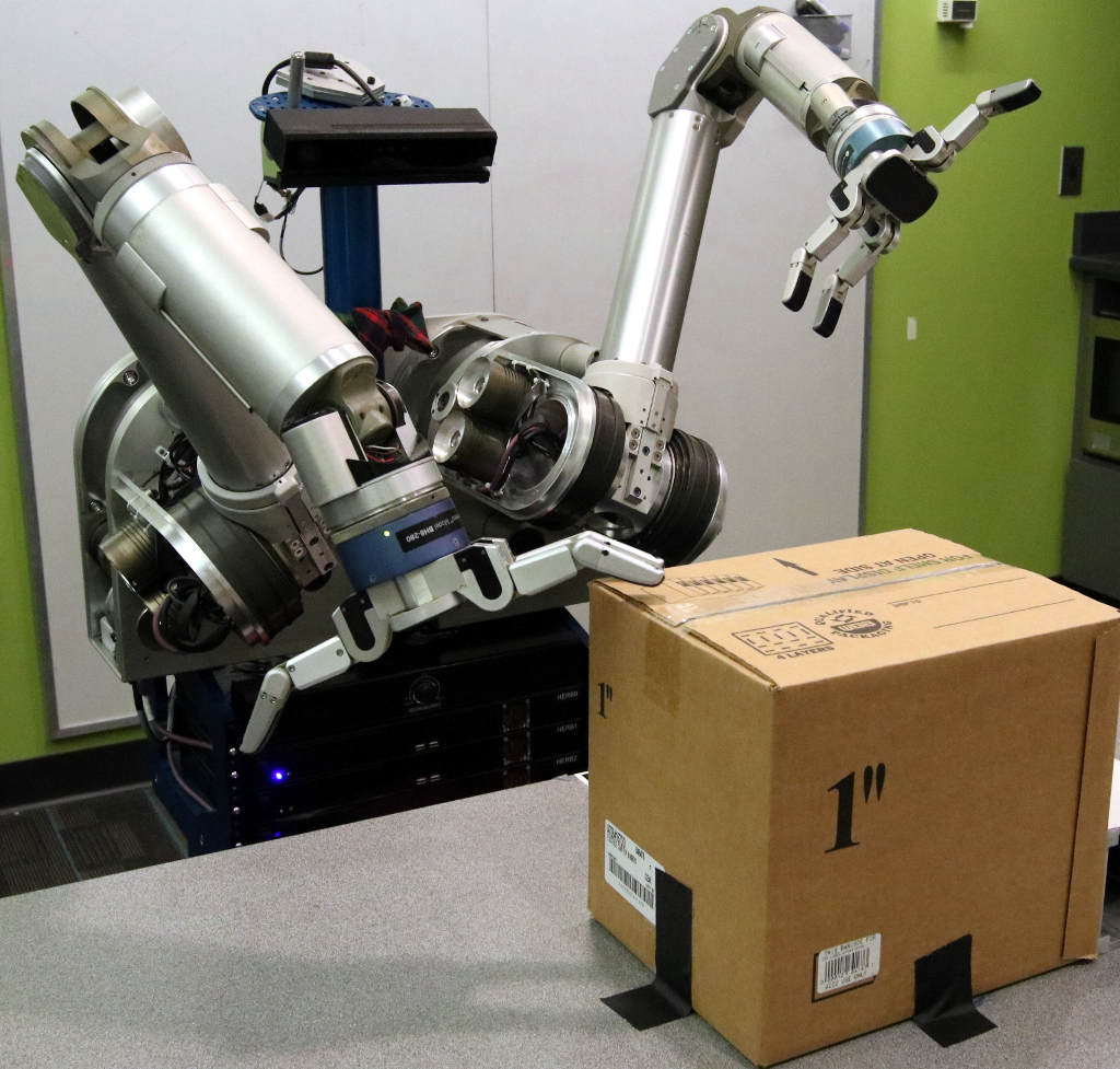
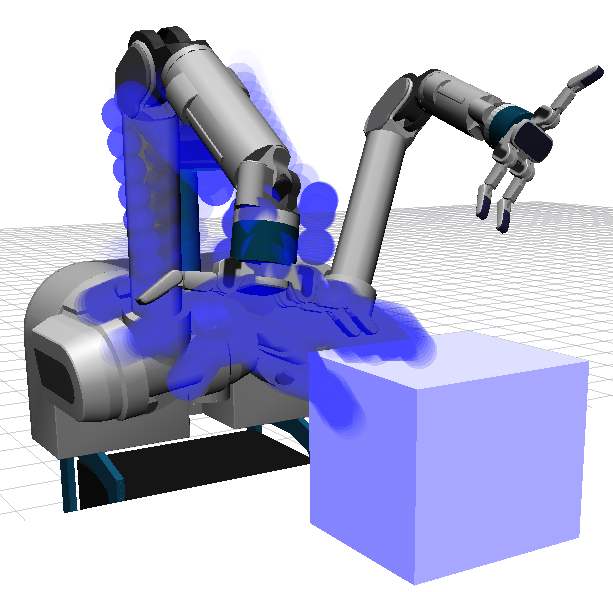
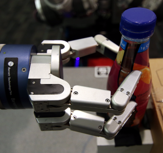
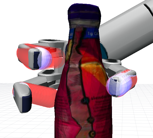
Figure 1: Two examples of imperfect proprioception. (Top) The Barrett WAM [2] touching a box. The solid render shows the configuration of the arm estimated by the WAM’s encoders and the blue renders are particles. Note that there are two modes in the distribution. (Bottom) The BarrettHand [3] grapsing a bottle with no position sensors on its distal joints. The solid render shows the configuration of the hand when the distal joints are assumed to be fixed. The red render shows the mode estimated from the particles.

Robots often have imperfect proprioception. This may arise from difficult-to-model transmissions, underactuated degrees of freedom, or poorly calibrated sensors. Fig. 1 (Top) shows a Barrett WAM arm [2] touching a box. The WAM measures its joint angles through a cable drive transmission that suffers from hysteresis related to stretch in the cables [4]. Fig. 1 (Bottom) shows the BarrettHand [3] grasping a bottle. The position of the distal finger joints depends on the state of a mechanical clutch that engages when a torque threshold is met.

In both cases, the nominal configuration reported by the robot is in error. In Fig. 1 (Top), the robot believes that it is several centimeters above the box even though a finger is in contact. In Fig. 1 (Bottom), the robot computed the configuration of its distal links under the assumption that the clutch did not engage even though all three fingers made contact with the object. In both cases, the nominal joint positions are inconsistent with the robot’s readings from its contact sensors.

Our goal is to use contact sensors to refine a robot’s estimate of its configuration. Like related work (Section II) dating back to the 1970s [5], we frame this as a problem of Bayesian estimation. State is the configuration of the robot, an action is a commanded change in configuration, and an observation is a measurement from the robot’s contact sensors (Section III). Under this formulation, a contact observation constrains the set of feasible states to a lower dimensional contact manifold that place the active sensors in non-penetrating contact with the environment.

Traditional Bayesian estimation techniques perform poorly on this domain. The extended [6] and unscented [7] Kalman filters assume a Gaussian distribution over state, which cannot accurately represent a set of feasible solutions on the contact manifold. The conventional particle filter (CPF) [8] suffers from particle deprivation because there the contact manifold has zero measure: there is zero probability of sampling a state from the ambient space that lies on it [1].

Instead, we use the manifold particle filter (MPF) [1]. The MPF is identical to the CPF when the robot has not sensed contact. When the robot does sense contact, the MPF samples particles from the contact manifold and re-weights them based on their proximity to the previous set of particles. The MPF has been successfully used to estimate the pose of an object relative to the hand during planar manipulation using explicit analytic and sample-based representations of the contact manifold.

Explicit representations of the contact manifold do not scale to the high-dimensional state space of this problem. Our key insight is to build an implicit representation of the contact manifold using a signed distance field (SDF) and constraint projection (Section IV). First, we sample a set of particles uniformly from the region of state space near the previous set of particles. Then, we use a SDF and the Jacobian of the manipulator to project the samples onto the manifold.

We demonstrate the efficacy of this technique in simulation (Section V) and real robot (Section VI) experiments for two problem domains. First, we consider a two, three, or seven degree-of-freedom arm with noisy positions sensors moving in a static environment. Second, we consider an underactuated robotic hand grasping a static object. In both cases, we show that the proposed technique significantly outperforms the CPF.

We believe that the proposed approach is applicable to a wide variety of problem domains. However, it has one key limitation: it requires a known, static environment. We plan to relax this assumption in future work by incorporating the pose of dynamic objects into the filter’s state space (Section VII).

II Related Work

There are a variety of approaches that use feedback from contact sensors for manipulation. One approach is to plan a sequence of move-until-touch actions that are guaranteed to localize an object to the desired accuracy [9, 10, 11] Other approaches formulate the problem as a partially observable Markov decision process [12] and solve for a policy that optimizes expected reward [13, 14, 15]. These algorithms require an efficient implementation of a Bayesian state estimator that can be queried many times during planning. Our approach could be used as a state estimator in one of these planners.

Recent work has used the conventional particle filter (CPF) [8] to estimate the pose of an object while it is being pushed using visual and tactile observations [16, 17]. Unfortunately, the CPF performs poorly because the set of feasible configurations lie on lower-dimensional contact manifold. The manifold particle filter (MPF) avoids particle deprivation by sampling from an approximate representation of this manifold [1]. However, building an explicit representation of the contact manifold is only feasible for low-dimensional—typically planar—problems.

In this work, we extend the MPF to estimate the full—typically six or more dimensional—configuration of a robot under proprioceptive uncertainty. Depth-based trackers, such as articulated ICP [18, 19], GMAT [20], and DART [21], can track the configuration of a robot using commercially available depth sensors. DART has been extended to incorporate contact observations using a method similar to our constraint projection [22]. However, all of these methods maintain a uni-modal state estimate and, thus, perform best when the robot is visible and un-occluded. In contrast, the MPF maintains a full distribution over belief space, only requires contact sensors, and is unaffected by occlusion.

The work most similar to our own aims to localize a mobile robot in a known environment using contact with the environment. Prior work has used the CPF to localize the pose of a mobile manipulator by observing where its arm contacts with the environment [23]. The same approach was used to localize a quadruped on known terrain by estimating the stability of the robot given its configuration [24]. Estimating the base pose of a mobile robot is equivalent to solving the problem formulated in this paper with the addition of a single, unconstrained six degree-of-freedom joint that attaches the robot to the world.

Techniques for estimating the configuration of an articulated body from contact sensors are applicable to humans as well as robots. Researchers in the computer graphics community have instrumented objects with contact sensors [25] and used multi-touch displays [26] to reconstruct the configuration of a human hand from contact observations. Both of these approaches generate natural hand configurations by interpolating between data points collected on the same device. Other work has used machine learning to reconstruct the configuration of a human from the ground reaction forces measured by pressure sensors [27]. We hope that our approach is also useful in these problem domains.

A recent work on robot state estimation from touch [28] estimates the robot’s joint angles and Denavit Hartenberg parameters from a single self-touch. Our work is related only insofar as we are estimating the joint angles of a robot arm using touch, but differs in that we use online filtering rather than batch optimization, and rather than estimating the state using one closed-chain self touch, we estimate the state using multiple open-chain touches of the environment.

III Background

Our approach is straightforward: as the robot moves around and contacts surfaces, we run a high-dimensional Manifold Particle Filter in its configuration space. Physical constraints from contact and collision with the robot’s body allow us to reason about how its joints have moved, compensating for joint angle noise.

III-A Problem Definition

Consider a robot with configuration space $Q=\mathbb{R}^{n}$. At each timestep the robot executes a control input $\mathbf{u}\in U$, transitions to the successor state $\mathbf{q}^{\prime}\sim p(\mathbf{q}^{\prime}|\mathbf{q},\mathbf{u})$, and receives an observation $\mathbf{z}\sim p(\mathbf{z}|\mathbf{q}^{\prime},\mathbf{u})$. An observation $\mathbf{z}=({\mathbf{q}_{\text{e}}},\mathbf{c})\in Z$ includes a noisy estimate ${\mathbf{q}_{\text{e}}}\in\mathbb{R}^{n}$ of the robot’s configuration and a binary vector of readings $\mathbf{c}\in\{0,1\}^{m}$ from the robot’s $m$ contact sensors.

Our goal is to estimate the belief state $\text{bel}(\mathbf{q}_{t})=p(\mathbf{q}_{t}|\mathbf{u}_{1:t},\mathbf{z}_{1:t})$, the probability distribution over the state $\mathbf{q}_{t}$ given the history of actions $\mathbf{u}_{1:t}=\mathbf{u}_{1},\dotsc,\mathbf{u}_{t}$ and observations $\mathbf{z}_{1:t}=\mathbf{z}_{1},\dotsc,\mathbf{z}_{t}$.

III-A1 Transition Model

Our method is applicable to any transition model where it is possible to sample from $p(\mathbf{q}^{\prime}|\mathbf{q},\mathbf{u})$ for given values of $\mathbf{q}$ and $\mathbf{u}$. In our experiments, we choose $\mathbf{u}$ to be commanded joint velocities and define

$$\mathbf{q}^{\prime}=\textbf{F}\left(\mathbf{q}+\operatorname{uniform}B\left(\mathbf{u},r_{a}\right)\Delta t\right)$$

as the noisy forward integration of the control input $\mathbf{u}$, where the noise is a uniform sample drawn from a ball $B$ of radius $r_{a}$. We assume that the world is static and does not change in response to the robot’s touch. In our experiments we use a simple physics simulation F involving frictionless soft collisions with the environment. As the robot touches the static environment, contact forces push it away from obstacles.

III-A2 Observation Model

We assume that proprioceptive and contact sensor observations are conditionally independent given the state $\mathbf{q}$ and most recent action $\mathbf{u}$. Under this assumption, we can express the observation model

$$p(\mathbf{z}|\mathbf{q},\mathbf{u}) =p({\mathbf{q}_{\text{e}}}|\mathbf{q},\mathbf{u})p(\mathbf{c}|\mathbf{q},\mathbf{u})$$

as the product of two marginal distributions.

The distribution $p({\mathbf{q}_{\text{e}}}|\mathbf{q},\mathbf{u})$ models uncertainty in the robot’s joint position sensors. We make no assumptions about the form of this distribution other than that it be possible to evaluate the probability density for given values of ${\mathbf{q}_{\text{e}}}$, $\mathbf{q}$, and $\mathbf{u}$. In our experiments, we model ${\mathbf{q}_{\text{e}}}$ as a measurement of $\mathbf{q}$ corrupted by a static (but unknown) joint offset

$$\mathbf{q}={\mathbf{q}_{\text{e}}}+{\Delta\mathbf{q}}$$

the initial offset ${\Delta\mathbf{q}}$ is sampled from a Gaussian at time $0$:

$${\Delta\mathbf{q}}\sim\mathcal{N}(0,\Sigma_{\Delta\mathbf{q}})$$

and remains static for the rest of the experiment. Therefore

$$p({\mathbf{q}_{\text{e}}}|\mathbf{q},\mathbf{u})=\mathcal{N}({\mathbf{q}_{\text{e}}}-\mathbf{q},\Sigma_{\Delta\mathbf{q}})$$

To model this, instead of estimating a belief over the full state $\mathbf{q}$, we estimate a belief over offsets ${\Delta\mathbf{q}}$ (the state being derivative of the offset and the joint encoders). It should be understood that whenever the state $\mathbf{q}$ is mentioned in this work, what is meant is $\mathbf{q}={\mathbf{q}_{\text{e}}}+{\Delta\mathbf{q}}$.

If one or more joints are unobserved, such as the distal joints in Fig. 1 (Bottom), then ${\mathbf{q}_{\text{e}}}$ has fewer dimensions than $\mathbf{q}$. We treat those unobserved dimensions of $\mathbf{q}$ as initially having uniform probability over the entire state space.

The distribution $p(\mathbf{c}|\mathbf{q},\mathbf{u})$ models the robot’s contact sensors. Each sensor is a rigid body that is attached to one of the robot’s links. The sensor returns “contact” if any part of the sensor touches the environment and otherwise returns “no contact.” Similar to prior work [1], we assume that the contact sensors do not generate false positives.

III-B Bayes Filter

The Bayes filter provides method of recursively constructing $\text{bel}(\mathbf{q}_{t})$ from $\text{bel}(\mathbf{q}_{t-1})$. Given an initial belief $\text{bel}(\mathbf{q}_{0})$, the Bayes filter applies the update rule

$$\text{bel}(\mathbf{q}_{t}) =\eta\,p(\mathbf{z}|\mathbf{q}_{t},\mathbf{u})\int_{Q}p(\mathbf{q}_{t}|\mathbf{q}_{t-1},\mathbf{u})\text{bel}(\mathbf{q}_{t-1})\,d\mathbf{q}_{t-1}$$

where $\eta$ is a normalization constant. This equation is derived from the definition of the belief state and the Markov property.

There are several ways of implementing the Bayes filter. The discrete Bayes filter represents $\text{bel}(\mathbf{q}_{t})$ as a piecewise constant histogram. Discretization is intractable on our problem $Q$ is typically high dimensional: $n\geq 6$ for a most manipulators. The Kalman filter, extended Kalman filter [6], and unscented Kalman filter [7] avoid discretization by assuming that $\text{bel}(\mathbf{q}_{t})$ is Gaussian. This assumption is not valid for our problem: the observation model $p(\mathbf{c}|\mathbf{q},\mathbf{u})$ is discontinuous and tends to produce multi-modal belief states.

III-C Conventional Particle Filter

Instead, we use the particle filter [8]. The particle filter (Alg. 1) is an implementation of the Bayes filter that represents $\text{bel}(s_{t})$ using a discrete set of weighted samples $Q_{t}=\{\langle\mathbf{q}_{t}^{[i]},w_{t}^{[i]}\rangle\}_{i=1}^{k}$, known as particles. The set of particles $Q_{t}$ at time $t$ is recursively constructed from the set of particles $X_{t-1}$ at time $t-1$ using importance sampling.

Input: $Q_{t-1}$ particles sampled from $\text{bel}(\mathbf{q}_{t-1})$

Output: $Q_{t}$ particles sampled from $\text{bel}(\mathbf{q}_{t})$

1

2$Q_{t}\leftarrow\emptyset$

3 for $\mathbf{q}_{t-1}^{[i]}\in Q_{t-1}$ do

4       $\mathbf{q}_{t}^{[i]}\sim p(\mathbf{q}_{t}|\mathbf{q}_{t-1}^{[i]},u_{t})$

5       $w_{t}^{[i]}\leftarrow p(\mathbf{z}|\mathbf{q}_{t}^{[i]},u_{t})$

6 end for

$Q_{t}\leftarrow\textsc{Resample}(Q_{t})$

Algorithm 1 Conventional Particle Filter

First, the particle filter samples a set of $k$ states $\mathbf{q}_{t}^{[i]}\sim\rho_{\text{conv}}(\mathbf{q})$ from a proposal distribution $\rho_{\text{conv}}(\mathbf{q})$. Conventionally, the proposal distribution is chosen to be

$$\rho_{\text{conv}}(\mathbf{q}_{t}) =\int_{Q}p(\mathbf{q}_{t}|\mathbf{q}_{t-1},\mathbf{u})\text{bel}(\mathbf{q}_{t-1})\,d\mathbf{q}_{t-1},$$ (1)

the transition model applied to the previous belief state. This can be implemented by forward simulating $Q_{t-1}$ to time $t$ using the transition model.

Next, the particle filter computes an importance weight $w_{t}^{[i]}=\text{bel}(\mathbf{q}_{t}^{[i]})/\rho_{\text{conv}}(\mathbf{q}_{t}^{[i]})$ to correct for the discrepancy between the proposal distribution $\rho_{\text{conv}}(\mathbf{q}_{t})$ and the desired distribution $\text{bel}(\mathbf{q}_{t})$. When using the proposal distribution shown in Eq. 1, the corresponding importance weight s $w_{t}^{[i]}=\eta\,p(\mathbf{z}_{t}|\mathbf{q}_{t}^{[i]},\mathbf{u}_{t})$. This can be thought of as updating $Q_{t}$ to agree with the most recent observation $\mathbf{z}_{t}$.

Finally, the particle filter periodically resamples each particle in $Q_{t}$ with replacement, with probability proportional to its weight. This process is known as sequential importance resampling (SIR) and is necessary to achieve good performance over long time horizons.

III-D Degeneracy of the Conventional Particle Filter

Prior work [1] has shown that the conventional particle filter (CPF) performs poorly with contact sensors because $\text{bel}(s_{t})$ collapses to a lower-dimensional manifold. This leads to particle deprivation during contact, where $w_{t}^{[i]}=0$ for all but a few particles, because it is vanishingly unlikely that a particle sampled from the transition model will lie on the zero measure contact manifold.

To see why this is the case, consider a 2D, two jointed and two linked robot with a single point contact sensor on its distal link Fig. 2. When the robot contacts the environment, the contact state of its sensor changes. Infinitesimal motion along the surface results in the same contact state, but Infinitesimal motion away from the surface results in a different contact state. The set of configurations with the same contact state locally form a manifold that is lower dimensional than the full state space.

III-E Manifold Particle Filter

The manifold particle filter (MPF, Alg. 2) avoids particle deprivation by operating in two modes [1]. When no contact is observed, particle deprivation is behaves identically to the CPF by sampling particles from the transition model and weighting them by the observation model. When contact is observed, the MPF switches to sampling particles from the observation model and weighting them by the transition model.

Both modes of the MPF implement importance sampling with different proposal distributions. During contact, the MPF samples particles from the dual proposal distribution

$$\rho_{\text{dual}}(\mathbf{q}_{t}) =\frac{p(\mathbf{z}_{t}|\mathbf{q}_{t},\mathbf{u}_{t})}{p(\mathbf{z}_{t}|\mathbf{u}_{t})},$$

where $p(\mathbf{z}_{t}|\mathbf{u}_{t})$ is a normalization constant. Sampling from $\rho_{\text{dual}}(\mathbf{q}_{t})$ generates configurations that are consistent with the most recent observation $\mathbf{z}_{t}$ according to the observation model. The remainder of this paper describes how to generate these samples efficiently.

The importance weight for a particle $\mathbf{q}_{t}^{[i]}\sim\rho_{\text{dual}}(\mathbf{q}_{t})$ is

$$w_{t}^{[i]} =\eta\int_{Q}p(\mathbf{q}_{t}|\mathbf{q}_{t-1},\mathbf{u})\text{bel}(\mathbf{q}_{t-1})\,d\mathbf{q}_{t-1}$$ (2)

where $\eta$ is another normalization constant. The importance weight $w_{t}^{[i]}$ incorporates information from $\text{bel}(\mathbf{q}_{t-1})$ into the posterior belief state; i.e. enforces temporal consistency with the transition model.

Computing $w_{t}^{[i]}$ exactly is not possible with a particle-based representation of $\text{bel}(\mathbf{q}_{t-1})$. Instead, we forward simulate the particles $Q_{t-1}$ by applying the transition model just like we do in the CPF. This set of particles $Q_{t-1}^{+}$ are distributed according to the right-hand side of Eq. 2. We approximate the weight $w_{t}^{[i]}$ using a kernel density estimate [29] built from $Q_{t-1}^{+}$.

Input: $\mathbf{u}_{t}$, $Q_{t-1}$ particles sampled from $\text{bel}(\mathbf{q}_{t-1})$

Output: $Q_{t}$ particles sampled from $\text{bel}(\mathbf{q}_{t})$

1

2$Q_{t}\leftarrow\emptyset$

3 for $\mathbf{q}_{t-1}^{[i]}\in Q_{t-1}$ do

4       if $\mathbf{c}_{t}=0$ then

5             $\mathbf{q}_{t}^{[i]}\sim p(\mathbf{q}_{t}|\mathbf{q}_{t-1}^{[i]},\mathbf{u}_{t})$

6             $w_{t}^{[i]}\leftarrow p(\mathbf{c}_{t}|\mathbf{q}_{t}^{[i]},\mathbf{u}_{t})$

7      else

8             $\mathbf{q}_{t}^{[i]}\sim\operatorname{uniform}M(\mathbf{c})$

9             $w_{t}^{[i]}\leftarrow\textsc{KernelDensityEstimate}(Q_{t-1}^{+},\mathbf{q}_{t}^{[i]})$

10       end if

11      

12 end for

13$Q_{t}\leftarrow\textsc{Resample}(Q_{t})$

Algorithm 2 Manifold Particle Filter

IV Implicit Contact Manifold Representation

Implementing the MPF requires sampling from the lower-dimensional contact manifold associated with the active contact sensors. In this section, we formally define the contact manifold (Section IV-A) associated with contact observation $\mathbf{c}$ and explain why it is infeasible to build an explicit representation of this manifold.

Instead, we implicitly define the contact manifold as the iso-contour of a loss function (Section IV-B) and use a local optimizer to project onto it (Section IV-C) by using a signed-distance field to compute gradient information (Section IV-D). Finally, we describe three different methods of using projection to sample from the observation model (Section IV-E).

IV-A Contact Manifold

Suppose the robot is in a static environment with obstacles $X_{\text{obs}}\subseteq\mathbb{R}^{3}$ with boundary $X_{\text{surf}}=X_{\text{obs}}\setminus\operatorname{int}(X_{\text{obs}})$. The robot’s $i$-th contact sensor is a rigid body with geometry $c(\mathbf{q})\subseteq\mathbb{R}^{3}$ in configuration $\mathbf{q}$. If the robot senses contact with sensor $i$, then we know that $c_{i}(\mathbf{q})$ is in non-penetrating contact with the environment; i.e. $c_{i}(\mathbf{q})\cap X_{\text{surf}}\neq\emptyset$.

We define the sensor contact manifold $M_{i}$ of sensor $i$ as

$$M_{i} =\{\mathbf{q}\in Q:c(\mathbf{q})\cap X_{\text{surf}}\neq\emptyset\},$$

the set of all configurations that put $c_{i}(\mathbf{q})$ in contact with the environment. If multiple contact sensors are active, then we know that all active sensors are in non-penetrating contact with the environment. Fig. 2(a) shows a simple example of this.

The observation contact manifold $M(\mathbf{c})$ is given by the intersection of the active sensor contact manifolds

$$M(\mathbf{c}) =\bigcap_{i\in\Phi(\mathbf{c})}M_{i},$$

where $\Phi(\mathbf{c})$ denotes the indices of the sensors active in $\mathbf{c}$.

Explicitly representing $M(\mathbf{c})$ for small problems. For example, Fig. 4(a) shows a 2D robot with two joints in an environment consisting of a single point. In this environment, the contact manifold can be computed easily using analytic inverse kinematics. However, as the environment and dimensionality of the problem increase in complexity (Fig. 4(b), Fig. 4(c)), deriving an explicit representation of the manifold becomes computationally infeasible, because it requires computing inverse kinematics solutions for every surface point which would cause the contact $\mathbf{c}$.

IV-B Implicit Representation of the Contact Manifold

Luckily for the MPF, we do not need to compute an explicit representation of $M(\mathbf{c})$: we only have to be able to draw samples from it. In this work, we first sample from the full state space, and then project onto the $M(\mathbf{c})$, which is only represented implicitly as the iso-contour of a loss function. We then reject any sample that is not close enough to the manifold.

We represent the sensor contact manifold $M_{i}$ as the zero iso-contour $M_{i}=\{\mathbf{q}\in Q:\operatorname{dist}(c_{i}(\mathbf{q}),X_{\text{obs}})=0\}$ of the signed distance function

$$\operatorname{dist}(X,Y) =\min_{x\in X}\begin{cases}\hphantom{-}\operatorname{dist}(x,Y)&:x\not\in Y\\ -\operatorname{dist}(x,Y)&:\text{otherwise}\end{cases}$$

between the sensor and the environment. A signed distance is a positive value equal to the distance between two disjoint sets or negative value equal to the deepest penetration between two intersecting sets. The signed distance $\operatorname{dist}(c_{i}(\mathbf{q}),X_{\text{obs}})$ is zero iff contact sensor $i$ is in non-penetrating contact with the environment in configuration $\mathbf{q}$.

A configuration $\mathbf{q}$ lies on the observation contact manifold $M(\mathbf{c})$ if the signed distance $\operatorname{dist}(c_{i}(\mathbf{q}),X_{\text{obs}})=0$ for all sensors active $i\in\Phi(\mathbf{c})$ in observation $\mathbf{c}$. We represent this set as the zero iso-contour $M(\mathbf{c})=\{\mathbf{q}\in Q:D_{\mathbf{c}}(\mathbf{q})=0\}$ of the loss function

$$D_{\mathbf{c}}(\mathbf{q}) =\sum_{i\in\Phi(\mathbf{c})}\left[\operatorname{dist}(c_{i}(\mathbf{q}),X_{\text{obs}})\right]^{2},$$

which is zero iff $\mathbf{q}\in M(\mathbf{c})$. Any function that satisfies this property is sufficient. We choose sum-of-squared distances to simplify the projection operator described below.

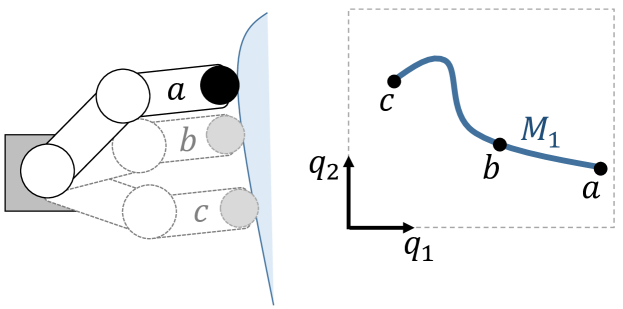
(a) Contact manifold

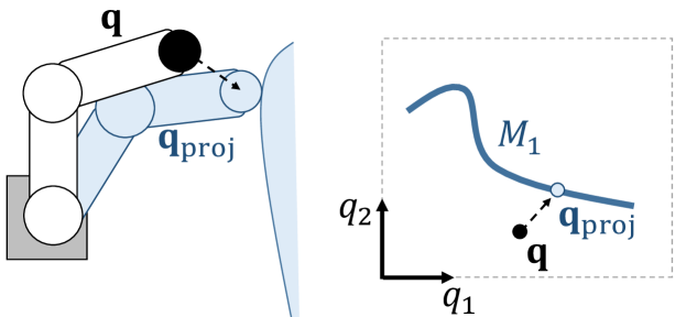
(b) Projection onto the contact manifold

Figure 2: Example of the contact manifold for a contact sensor (black circle) on a planar, two degree-of-freedom robot. The robot’s configuration space, parameterized by the two joint angles $q_{1}$ and $q_{2}$ is shown on the right. (2(a)) Three different configurations $a$, $b$, and $c$ that lie on the contact manifold $M_{1}$. (2(b)) The configuration $\mathbf{q}$ is projected to a nearby configuration $\mathbf{q}_{\text{proj}}$ that lies on $M_{1}$.

IV-C Projecting onto the Contact Manifold

We project a sample from the ambient space $\mathbf{q}$ onto the the contact manifold $M(\mathbf{c})$ by solving the optimization problem

$$\operatorname{proj}(\tilde{\mathbf{q}},\mathbf{c}) =\operatornamewithlimits{arg\,min}_{\mathbf{q}\in N(\tilde{\mathbf{q}})}D_{\mathbf{c}}(\mathbf{q})$$ (3)

in a neighborhood $N(\tilde{\mathbf{q}})\subseteq Q$ around an initial configuration $\tilde{\mathbf{q}}\in Q$. If the distance $D_{\mathbf{c}}(\mathbf{q})=0$ at the end of the optimization, then we have found a configuration $\mathbf{q}\in M(\mathbf{c})$. Fig. 2(b) shows an example of the outcome of this process.

We implement the minimization in Eq. 3 using simple gradient descent optimization. The optimizer is initialized with $\mathbf{q}^{(0)}=\tilde{\mathbf{q}}$ and iteratively applies the update rule

$$\mathbf{q}^{(j+1)} =\mathbf{q}^{(j)}-\lambda\nabla D_{\mathbf{c}}^{T}D_{\mathbf{c}}(\mathbf{q}^{(j)})$$

until $\mathbf{q}^{(j)}$ has converged, where $\lambda$ is the learning rate. Performing this update requires computing the gradient

$$\nabla D_{\mathbf{c}} =\nabla_{\mathbf{q}}\operatorname{dist}\mathbf{c}(\mathbf{q}) =2\sum_{i\in\Phi(\mathbf{c})}\nabla_{\mathbf{q}}\operatorname{dist}(c_{i}(\mathbf{q}),X_{\text{obs}}),$$

which, in turn, requires computing the gradient of the signed distance function. We describe how to efficiently compute $\operatorname{dist}(\cdot,\cdot)$ and $\nabla_{\mathbf{q}}\operatorname{dist}(\cdot,\cdot)$ in the next section.

Note that this procedure may converge to a configuration where $D_{\mathbf{c}}(\mathbf{q})\geq\epsilon$ because (1) there is no solution in the neighborhood $N(\tilde{\mathbf{q}})$ or (2) the optimizer reached a local minimum. In either case, the projection fails and needs to be re-initialized with a different $\tilde{\mathbf{q}}\in Q$.

This method of projecting onto the contact manifold using an implicit representation is commonly used in computer graphics to quickly compute contacts for simulated collision resolution and inverse kinematics. The method described here for computing an implicit contact manifold for an articulated body is essentially the same as one described in [30].

IV-D Signed Distance Computation

Evaluating $D_{\mathbf{c}}(\mathbf{q})$ requires computing the distance $\operatorname{dist}(c_{i}(\mathbf{q}),X_{\text{obs}})$ between each contact sensor $c_{i}(\mathbf{q})$ and the environment $X_{\text{obs}}$. Computing this distance metric is difficult and, potentially computationally expensive, for arbitrary geometric shapes. To avoid this, we approximate the static environment, which may contain arbitrary geometry, with a voxel grid and each contact sensors with a collection of geometric primitives (e.g. spheres, capsules, boxes).

As an offline pre-computation step, we compute a discrete signed distance field over the voxel grid using the technique from Felzenszwalb and Huttenlocher [31]. A signed distance field (SDF) is a function $\Phi:x\in\mathbb{R}^{3}\mapsto\operatorname{dist}(x,X_{\text{obs}})$ that maps each point $x$ in the workspace to its signed distance to the nearest obstacle. Fig. 3 shows an example of a SDF computed in built in this way.

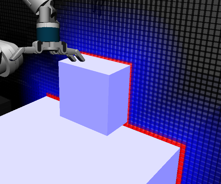
Figure 3: Visualizing a two-dimensional slice of the signed distance field (SDF) $\Phi(\cdot)$. Blue voxels have $\Phi(\cdot)>0$ and red voxels have $\Phi(\cdot)\leq 0$. Precomputing this SDF takes between two and five seconds. The voxel grid has a 2 cm resolution.

Without loss of generality, assume that the geometry of each contact sensor is a sphere with center $\mathbf{p}_{i}(\mathbf{q})\in Q$ and radius $r_{i}$. The signed distance between the sensor and the environment is given by

$$\operatorname{dist}(c_{i}(\mathbf{q}),X_{\text{obs}}) =\Phi(\mathbf{p}_{i}(\mathbf{q}))-r_{i}.$$

The gradient of the distance is given by

$$\nabla_{\mathbf{q}}\operatorname{dist}(c_{i}(\mathbf{q}),X_{\text{obs}}) =-\left[\Phi(\mathbf{p}_{i}(\mathbf{q}))-r_{i}\right]\left[J_{i}(\mathbf{q})\right]^{T}\nabla_{\mathbf{x}}\Phi(\mathbf{p}_{i}(\mathbf{q})),$$

where $J_{i}(\mathbf{q})=\frac{\partial\mathbf{p}_{i}}{\partial\mathbf{q}}$ is the linear Jacobian of the manipulator. We approximate the gradient $\nabla_{\mathbf{x}}\Phi(\mathbf{p}_{i}(\mathbf{q}))$ of the SDF with a finite difference.

Critically, evaluating $\Phi(\cdot)$ requires a single memory lookup and evaluating the gradient $\Delta_{x}\Phi(x)$ can be efficiently approximated by a finite difference. This is the same representation of the environment used by CHOMP, a gradient-based trajectory optimizer [32].

IV-E Sampling from the Contact Manifold via Projection

The projection operator described above starts with a single initial configuration $\tilde{\mathbf{q}}\in Q$ and projects it onto the contact manifold $M(\mathbf{c})$. Sampling from the dual proposal distribution requires $n$ such samples distributed uniformly over $M(\mathbf{c})$. We describe three different approaches for selecting the set of initializations $\tilde{Q}_{t}=\{\tilde{\mathbf{q}}^{[i]}\}_{i=1}^{n}$ used to generate the set of particles $Q_{t}$. If a projection operation fails, i.e. $D_{\mathbf{c}}(\mathbf{q}^{[i]})\geq\epsilon$, then we generate a new initialization $\tilde{\mathbf{q}}^{[i]}$ and try again.

IV-E1 Uniform Projection

The simplest strategy is to sample $\tilde{\mathbf{q}}^{[i]}\sim\operatorname{uniform}(Q)$ uniformly from the robot’s configuration space. This method is unbiased with respect to the previous set of particles $Q_{t-1}$. Unfortunately, since $Q$ is high dimensional, it may take a large number of particles to adequately cover the the manifold. This may lead to particle deprivation.

IV-E2 Particle Projection

We can focus our samples near $Q_{t-1}$ by directly projecting the previous set of particles $\tilde{Q}_{t}=Q_{t-1}$ onto the contact manifold. This method tightly focuses samples on the portions of the manifold that will be assigned high importance weights. However, this comes with two downsides: (1) $Q_{t}$ will have a non-uniform distribution (2) the set of particles may have size $|Q_{t}|<n$ if projecting any particles fails.

IV-E3 Ball Projection

We can combine the advantages of both approaches by uniformly sampling particles $\tilde{\mathbf{q}}_{t}\sim\operatorname{uniform}R(Q_{t-1})$ from the region of configuration space $R(Q_{t-1})$ near the previous set of particles $Q_{t-1}$. We define the region

$$R(Q_{t-1}) =\bigcup_{\mathbf{q}^{[i]}\in Q_{t-1}}B_{r_{\epsilon}}(\mathbf{q}^{[i]})$$

where $B_{r_{\epsilon}}(\mathbf{q}^{[i]})=\{\mathbf{q}\in Q:||\mathbf{q}-\mathbf{q}^{[i]}||<r_{\epsilon}\}$ is a ball centered at $\mathbf{q}^{[i]}$ with radius $r_{\epsilon}$. The set $R(Q_{t-1})$ is the union of all such balls centered at the particles in $Q_{t-1}$.

This approach is equivalent to particle projection as $r_{\epsilon}\to 0$. and equivalent to uniform projection as $r_{\epsilon}\to\infty$. We select the radius $r_{\epsilon}$ such that the transition model has probability $\operatorname{Pr}(\mathbf{q}^{\prime}\not\in R(Q_{t-1}))<\epsilon$ of generating a successor state $\mathbf{q}^{\prime}\sim p(\mathbf{q}^{\prime}|\mathbf{q},\mathbf{u})$ outside of $R(Q_{t-1})$ given any $\mathbf{q}\in Q_{t-1}$. For this choice of $r_{\epsilon}$, this approach is an $\epsilon$-approximation of the uniform sampling method. However, this approach concentrates the particles $Q_{t}$ concentrated on the region of $M(\mathbf{c})$ with high importance weights.

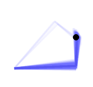
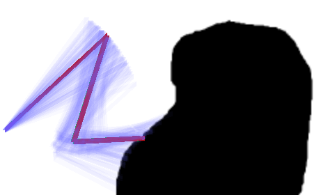
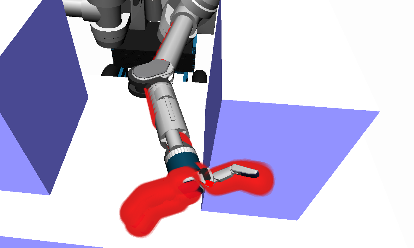
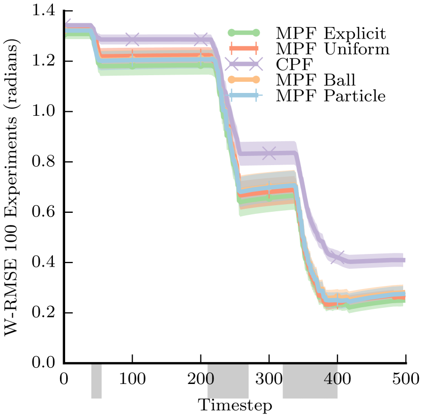
(a) 2-DOF Simulation.

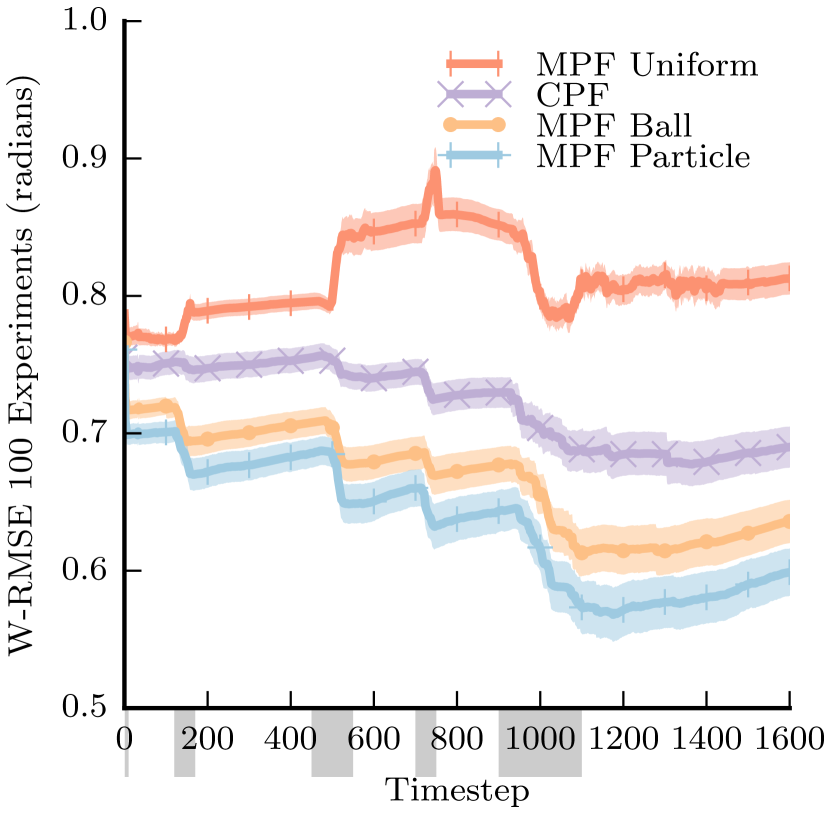
(b) 3-DOF Simulation.

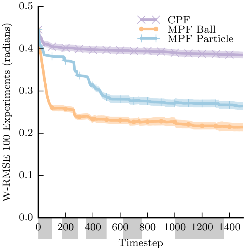
(c) 7-DOF Simulation.

Figure 4: Filter performance using simulated data with 250 particles. Top row: the 2-DOF, 3-DOF and 7-DOF simulations. Bottom row: filter performance. Periods of persistent contact (in any experiemnt) are shaded grey on the $x$ axis. The weighted root mean square error is shown over 100 experiments with randomized starting conditions drawn from the prior, the $95\%$ confidence interval is lightly shaded.

V Simulation Experiments

V-A Experimental Design

We evaluate an estimator by performing a number of trials where we draw an initial state $\mathbf{q}_{0}\sim\text{bel}(\mathbf{q}_{0})$ from the initial belief state $\text{bel}(\mathbf{q}_{0})$ and forward-simulate $\mathbf{q}_{t+1}\sim p(\mathbf{q}_{t+1}|\mathbf{q}_{t},\mathbf{u}_{t})$ through a pre-defined sequence of $T$ actions $\mathbf{u}_{1},\dotsc,\mathbf{u}_{T}$. After each timestep, we draw an observation $\mathbf{z}_{t}\sim p(\mathbf{z}_{t}|\mathbf{q}_{t},\mathbf{u}_{t})$ from the observation model.

The estimator returns a set of particles $Q_{t}$ at each timestep. We measure the accuracy of this estimate by computing the weighted root mean square error (W-RMSE)

$$\text{W-RMSE}(\mathbf{q}_{t},Q_{t}) =\sqrt{\frac{\sum_{i=1}^{k}w_{t}^{[i]}||\mathbf{q}_{t}^{[i]}-\mathbf{q}_{t}||^{2}}{\sum_{i=1}^{k}w_{t}^{[i]}}}.$$

We average W-RMSE over 100 trials with different initial states.

We considered three different environments:

V-B Two-Dimensional 2-DOF Arm

First, we consider a two degree-of-freedom arm in a two-dimensional environment containing a single point obstacle (Fig. 4(a)). We set $\Sigma_{\Delta\mathbf{q}}=2.0(\mathbf{I})$. The robot executes a series of velocity commands that bring it into contact with the obstacle several times. The noise in the motion model $r_{a}=0.05$ rad. It tracks its belief with $k=250$ particles.

The robot has a point contact sensor on the tip of its manipulator. The contact manifold always consists of two points in configuration space. Our simulation results confirm this: the robot was able to reduce most of its uncertainty in two touches. The first touch constrains the robot to one of two configurations. The second touch disambiguates between those configurations. This also allows us to implement MPF-Explicit by solving for an analytic solution to the robot’s inverse kinematics.

The CPF performed poorly due to particle deprivation. The contact manifold has zero measure, so the probability of sampling a particle near the manifold is low and the CPF collapses to one (possibly incorrect) mode. All MPF variants significantly outperform the CPF, but perform similarly: the contact manifold is small, so a small number of samples is sufficient to densely cover it.

V-C Two-Dimensional 3-DOF Arm

Next, we consider a three degree-of-freedom arm in a two-dimensional environment that contains a large, unstructured obstacle (Fig. 4(b)). The robot has 20 circular contact sensors spaced evenly along its outer two links. We set $\Sigma_{\Delta\mathbf{q}}=0.8(\mathbf{I})$ The robot executes a series of human-controlled velocity commands that cause it to come into contact with and, in some cases,slide along the obstacle. The motion model noise $r_{a}=0.05$ rad. The robot tracks its belief with $k=250$ particles.

The results show that MPF-Particle and MPF-Ball perform significantly better than CPF, but MPF-Uniform performs worse. We cannot implement MPF-Explicit in this domain because of the complex shape of the obstacle. MPF-Uniform suffers from particle deprivation because the contact manifold is too large to cover densely with $250$ particles.

Surprisingly, MPF-Particle slightly outperforms MPF-Ball in this domain. We hypothesize that occurs because the robot maintains long periods of persistent contact with the obstacle. Prior work has shown that the kernel density estimation step of the MPF introduces additional variance into the belief state during persistent contact [1]. This is partially masked by the local optimization performed by MPF-Particle.

V-D Three-Dimensional 7-DOF Arm

Finally, we consider a simulated seven degree-of-freedom Barrett WAM [2] equipped with a BarrettHand [3] end-effector simulated by the Dynamic Animation and Robotics Toolkit (DART) [33]. The BarrettHand is kept in a fixed configuration and the environment contains of two large boxes in front of the robot. The robot has spherical contact sensors (not shown in the figure) on its fingers, wrist, and forearm. We set $\Sigma_{\Delta\mathbf{q}}=0.5(\mathbf{I})$. The robot executes a deterministic series of velocity commands that cause it to touch the environment and slide along it. A small amount of uniform noise ($r_{a}=0.01$ rad) is used in the motion model. 250 particles are used to track the belief.

The results show that MPF-Ball and MPF-Particle both outperform CPF. It is not possible to implement MPF-Explicit in this domain. MPF-Uniform is omitted from the plot because its large error would distort the scale. In this domain, MPF-Ball significantly outperforms MPF-Particle because the bias introduced by a direct projection step prevents the filter from finding a good solution. All filters perform in real-time (Table  I), with most of the time spent computing the observation model (resampling and projection to the contact manifold). MPF-Uniform is particularly slow because it must continually reject samples that fail to project to the manifold.

Algorithm	Total	Transition	Observation
CPF	$4\pm 1$ ms	$3\pm 1$ ms	$1\pm 1$ ms
MPF-Particle	$9\pm 7$ ms	$2\pm 1$ ms	$8\pm 7$ ms
MPF-Ball	$10\pm 7$ ms	$2\pm 1$ ms	$8\pm 8$ ms
MPF-Uniform	$35\pm 12$ ms	$2\pm 1$ ms	$34\pm 12$ ms

TABLE I: Timing data for the 7-DOF simulation (Fig. 4(c)), times shown in milliseconds with $95\%$ confidence interval. The total time is broken into its component transition and observation model updates. Only iterations of the filter where the robot was in contact are recorded. Time was recorded on a consumer laptop with an Intel core i7 CPU.

VI Real-Robot Experiments

We validated our simulation results in two real-robot experiments on a 7-DOF Barrett WAM [2] equipped with a BarrettHand [3] end-effector; the same platform simulated in the 7-DOF simulation experiments. Each finger of the BarrettHand’s three fingers contain a strain gauge that measures torque around the distal joint. The robot detects contact with the environment by thresholding changes in measurements reported by these sensors. We treat this value as a binary observation of contact anywhere on the distal finger link.

VI-A Arm Configuration Estimation

In the first experiment, we consider the robot’s arm configuration to be uncertain. We tele-operated the robot to execute a trajectory in an environment similar to the one described in Section V-D. We use the positions measured by the WAM’s motor encoders, which are located before the cable drive transmission, as proprioceptive observations ${\mathbf{q}_{\text{e}}}$. We measure the ground truth position of the arm using optical joint encoders installed after the cable drive transmission. These measurements are only used for evaluation purposes and are not available to the estimator.

Our goal is to estimate the 7-DOF configuration of the arm. Here, $\Sigma_{\Delta\mathbf{q}}=0.1(\mathbf{I})$. Fig. 5(a) shows one run of the experiment with $k=100$ particles, with $r_{a}=0.01$  rad. The results from this single experiment mirror those from Section V-D: both variants of MPF outperform CPF and MPF-Ball significantly outperforms MPF-Particle.

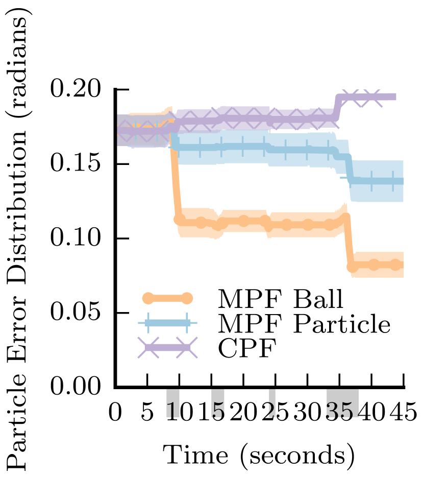
(a) Noisy arm.

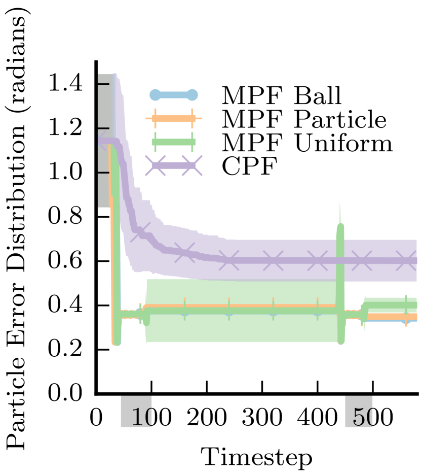
(b) Underactuated hand.

Figure 5: Experiments with real robot data (Fig. 1) with 250 particles. One run is shown with the mean error and standard deviation of the particle distribution for each filter. The $x$-axis is lightly shaded in grey wherever the robot is in persistent contact.

VI-B Underactuated Hand State Estimation

In the second experiment, the arm is held in a static configuration and the robot closes its hand around an object with a known pose. The BarrettHand [3] is underacutated: each finger has two joints that are coupled by a mechanical clutch. We assume that the proximal joint angles are known, but the distal joint angles are not. We record the ground truth distal joint angles using joint encoders for evaluation purposes, but do not make this data available to the estimator. The resolution of the SDF voxel grid was set to $10$ mm.

Our goal is to estimate the 3-DOF configuration of the distal finger joints. We chose the initial belief state to be a uniform distribution over a ball with radius $1$ rad centered at the origin of configuration space. Fig. 5(b) shows data from one trial that contains two grasps: one from $t\approx 40$ to $t\approx 100$ and another from $t\approx 450$ to $t\approx 500$.

The data shows that all variants of the MPF significantly outperform the CPF, but there is no significant difference between MPF-Uniform, MPF-Particle, and MPF-Ball. This is consistent with our results in the two-dimensional planar domain (Section V-B): this is a relatively simple problem because each of the three joints is part of an independent kinematic chain.

We were surprised to see that the touches introduced large transients in the MPF particle distribution, especially for MPF-Uniform. We believe that these are caused by latency in the strain gauge sensors that is not accounted for in our observation model.

VII Discussion and Future Work

We have shown how the MPF can be extended to high dimensional state spaces by implicitly representing the contact manifold with an objective function. Our simulation and real-robot results show that this approach outperforms the conventional particle filter in a number of scenarios. This approach can be used to compensate for proprioceptive error in a manipulator or to estimate the configuration of an underactuated robotic hand.

However, our approach has a key limitation: it requires a known, static environment. We could relax this requirement by incorporating the pose of movable objects in the environment—including the base pose of the robot—into the estimator’s state space. This is challenging because: (1) it is no longer possible to pre-compute a signed distance field and (2) the behavior of the projection depends on the parameterization of this configuration state space. We plan to explore these challenges in future work.

Finally, even though an implicit representation of the contact manifold allows us to sample from it efficiently, the samples we draw are biased by the fact that uniform samples of the ambient space will not project uniformly onto the contact manifold for two reasons: (1) because the measures of the full state space and the contact manifold may differ (a problem that even an explicit representation of the contact manifold suffers from) and (2) because projecting samples from the full state space to the contact manifold introduces bias. Our experiments have so far not made clear to what extent this bias degrades performance of the filter. One way of eliminating bias might be by rejecting and resampling particles that fail to meet some criterion of uniformity (e.g. Poisson disc sampling). An alternative solution might be sampling from the tangent space of the manifold rather than projecting to it [34].

References

- [1] M. Koval, N. Pollard, and S. Srinivasa, “Pose estimation for planar contact manipulation with manifold particle filters,” International Journal of Robotics Research, vol. 34, no. 7, pp. 922–945, 2015.
- [2] K. Salisbury, W. Townsend, B. Eberman, and D. DiPietro, “Preliminary design of a whole-arm manipulation system (WAMS),” in IEEE International Conference on Robotics and Automation, 1988.
- [3] W. Townsend, “The BarrettHand grasper–programmably flexible part handling and assembly,” Industrial Robot: An International Journal, vol. 27, no. 3, pp. 181–188, 2000.
- [4] B. Boots, A. Byravan, and D. Fox, “Learning predictive models of a depth camera & manipulator from raw execution traces,” in IEEE International Conference on Robotics and Automation, 2014.
- [5] S. Simunovic, “An information approach to parts mating,” Ph.D. dissertation, Massachusetts Institute of Technology, 1979.
- [6] R. Kalman, “A new approach to linear filtering and prediction problems,” Journal of Basic Engineering, 1960.
- [7] S. Julier and J. Uhlmann, “A new extension of the Kalman filter to nonlinear systems,” in International Symposium on Aerospace/Defense Sensing, Simulation, and Controls, 1997.
- [8] N. Gordon, S. D.J., and A. Smith, “Novel approach to nonlinear/non-Gaussian Bayesian state estimation,” in IEE Proceedings F, 1993.
- [9] A. Petrovskaya and O. Khatib, “Global localization of objects via touch,” IEEE Transactions on Robotics, vol. 27, no. 3, pp. 569–585, 2011.
- [10] S. Javdani, M. Klingensmith, J. Bagnell, N. Pollard, and S. Srinivasa, “Efficient touch based localization through submodularity,” in IEEE International Conference on Robotics and Automation, 2013.
- [11] P. Hebert, T. Howard, N. Hudson, J. Ma, and J. Burdick, “The next best touch for model-based localization,” in IEEE International Conference on Robotics and Automation, 2013.
- [12] R. Smallwood and E. Sondik, “The optimal control of partially observable Markov processes over a finite horizon,” Operations Research, vol. 21, no. 5, pp. 1071–1088, 1973.
- [13] K. Hsiao, L. Kaelbling, and T. Lozano-Pèrez, “Grasping POMDPs,” in IEEE International Conference on Robotics and Automation, 2007.
- [14] M. Horowitz and J. Burdick, “Interactive non-prehensile manipulation for grasping via POMDPs,” in IEEE International Conference on Robotics and Automation, 2013.
- [15] M. Koval, N. Pollard, and S. Srinivasa, “Pre- and post-contact policy decomposition for planar contact manipulation under uncertainty,” in Robotics: Science and Systems, 2014.
- [16] L. Zhang and J. Trinkle, “The application of particle filtering to grasping acquisition with visual occlusion and tactile sensing,” in IEEE International Conference on Robotics and Automation, 2012.
- [17] L. Zhang, S. Lyu, and J. Trinkle, “A dynamic Bayesian approach to simultaneous estimation and filtering in grasp acquisition,” in IEEE International Conference on Robotics and Automation, 2013.
- [18] S. Pellegrini, K. Schindler, and D. Nardi, “A generalisation of the ICP algorithm for articulated bodies,” in British Machine Vision Conference, vol. 3, 2008, p. 4.
- [19] M. Krainin, P. Henry, X. Ren, and D. Fox, “Manipulator and object tracking for in-hand 3D object modeling,” International Journal of Robotics Research, vol. 30, no. 11, pp. 1311–1327, 2011.
- [20] M. Klingensmith, T. Galluzzo, C. Dellin, M. Kazemi, J. Bagnell, and N. Pollard, “Closed-loop servoing using real-time markerless arm tracking,” in IEEE International Conference on Robotics and Automation Humanoids Workshop, 2013.
- [21] T. Schmidt, R. Newcombe, and D. Fox, “DART: Dense articulated real-time tracking,” in Robotics: Science and Systems, 2014.
- [22] T. Schmidt, K. Hertkorn, R. Newcombe, Z. Marton, M. Suppa, and D. Fox, “Depth-based tracking with physical constraints for robot manipulation,” in IEEE International Conference on Robotics and Automation, 2015.
- [23] M. R. Dogar, V. Hemrajani, D. Leeds, B. Kane, and S. Srinivasa, “Proprioceptive localization for mobile manipulators,” Robotics Institute, Carnegie Mellon University, Tech. Rep. CMU-RI-TR-10-05, 2010.
- [24] P. V. Sachin Chitta and, R. Geykhman, and D. D. Lee, “Proprioceptive localization for a quadrupedal robot on known terrain,” in IEEE International Conference on Robotics and Automation, 2007.
- [25] P. G. Kry and D. K. Pai, “Interaction capture and synthesis,” ACM Transactions on Graphics, vol. 25, no. 3, 2006.
- [26] S.-J. Chung, J. Kim, S. Han, and N. S. Pollard, “Quadratic encoding for hand pose reconstruction from multi-touch input,” in Eurographics Short Paper, 2015.
- [27] S. Ha, Y. Bai, and C. K. Liu, “Human motion reconstruction from force sensors,” in ACM SIGGRAPH/Eurographics Symposium on Computer Animation, 2011.
- [28] A. Roncone, M. Hoffmann, U. Pattacini, and G. Metta, “Automatic kinematic chain calibration using artificial skin: self-touch in the icub humanoid robot,” in Robotics and Automation (ICRA), 2014 IEEE International Conference on. IEEE, 2014, pp. 2305–2312.
- [29] M. Rosenblatt, “Remarks on some nonparametric estimates of a density function,” The Annals of Mathematical Statistics, vol. 27, no. 3, pp. 832–837, 1956.
- [30] H. Tian, X. Zhang, C. Wang, J. Pan, and D. Manocha, “Efficient global penetration depth computation for articulated models,” Computer-Aided Design, vol. 70, pp. 116 – 125, 2016, {SPM} 2015. [Online]. Available: http://www.sciencedirect.com/science/article/pii/S0010448515001074
- [31] P. F. Felzenszwalb and D. P. Huttenlocher, “Distance transforms of sampled functions,” Cornell Computing and Information Science, Tech. Rep., 2004.
- [32] N. Ratliff, M. Zucker, J. A. Bagnell, and S. Srinivasa, “Chomp: Gradient optimization techniques for efficient motion planning,” in Robotics and Automation, 2009. ICRA ’09. IEEE International Conference on, May 2009, pp. 489–494.
- [33] “Dynamic Animation and Robotics Toolkit,” http://dartsim.github.io, 2013.
- [34] H. Snoussi, “Particle filtering on riemannian manifolds. application to covariance matrices tracking,” in Matrix Information Geometry, 2013, pp. 427–449.