It from Knot

Abstract

Knot physics is the theory of the universe that not only unified all the fundamental interactions but also explores the underlying physics of quantum mechanics. In knot physics, the most important physical result is the unification of everything (including matter, motion, interaction and space-time, …) into the entanglement between vortex-membranes: our universe is a projection of a four three dimensional entangled vortex-membranes in five dimensional inviscid incompressible fluid, of which the low energy effective theory not only reproduces the Standard model – an $\mathrm{SU}_{\mathrm{strong}}\mathrm{(3)}\otimes\mathrm{SU}_{\mathrm{weak}}\mathrm{(2)}\otimes$U_Y(1) gauge theory but also leads to the physics of general relativity. In a word, it from knot.

I Introduction

In modern physics, quantum physics including quantum mechanics and quantum field theory describes the universe. In the framework of quantum field theory, it is believed that the interaction comes from exchanging virtual bosons via local gauge symmetry principles. The Standard model (an $\mathrm{SU_{\mathrm{strong}}(3)}\otimes\mathrm{SU}_{\mathrm{weak}}\mathrm{(2)}\otimes$U_Y(1) gauge theory with Higgs mechanism due to spontaneous symmetry breaking) is a special type of quantum field theory that focuses on three non-gravitational interactions: weak interaction, strong interaction, and electromagnetic interactionstand . On the other hand, to understand gravitational interaction, the general relativity is developed by Einstein that provides a unified description of gravity as a geometric property of space-time.

A Theory of Everything (TOE) to unify all interactions is a dream of physicists. There are several approaches towards TOE. String theory is a possible theory of TOEss . According to string theory, quantum matter consists of vibrating strings (or strands) and different oscillatory patterns of strings become different particles with different masses. For the researcheres on string theory, the key point can be summarized into ”it from string”. In condensed matter physics, the idea of our universe as an “emergent” phenomenon has become increasingly popular. In emergence approach, a deeper and unified understanding of the universe is developed based on a complicated many-body system with long range entanglement. This is the idea of ”it from qubit”. Different quantum fields correspond to different many-body systems: the vacuum corresponds to the ground state and the elementary particles correspond to the excitations of the systemswen . In addition, there exist many other proposals of TOE from different points of view, such as loop quantum gravity theoryloop , G. Lisi’s E8 theorye8 , C. Schiller’s Strand ModelStrand , R. Penrose’s twistor theorytwistor , Grigory E. Volovik’s emergent theory in liquid heliumvo …

In this paper, we point out a new approach – knot physics towards understanding our universekou1 ; kou2 ; kou3 . This paper summarizes the earlier three long papers, kou1 ; kou2 ; kou3 . In knot physics, our universe is a projection of four entangled three-dimensional vortex-membranes in five dimensional inviscid incompressible fluid. The collective motions of this system are described by fermionic elementary particles (different types of knots) and gauge fields. In particular, all four types of fundamental interactions (electromagnetic, weak, strong and gravitational interactions) are unified into single simple framework – knot. That means, ”it from knot”.

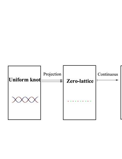
Figure 1: The framework structure of knot physics

II The foundation of knot physics

Fig.1 is the framework structure of knot physics. In this figure, we take a one dimensional (1D) knot with two entangled vortex-membranes as an example. Our starting point is a knot Under projection, the knot turns into zero-lattice. In the continuum limit, the effective theories of zero-lattice become quantum field theories. We show the correspondence between modern physics and knot physics as,

The universe $$\iff\text{ Entangled vortex-membranes }$$

(A uniform knot),

The space-time $$\iff\text{ 3+1D zero-lattice,}$$

Matter $$\iff\text{ Extra zeroes,}$$

Motion $$\iff\text{ The changing of the zero distribution,}$$

Quantum mechanics $$\iff\text{ Geometric Biot-Savart mechanics}$$

for extra zeroes.

Here, $\Longleftrightarrow$ denotes the correspondence between modern physics and knot physics.

The following points are foundation of knot physics.

Vortices are extended objects with singular vorticity in divergence-free inviscid incompressible fluid that can be regarded as a closed oriented embedded subvortex-membrane with Marsden-Weinstein (MW) symplectic structureleap . For two dimensional (2D) inviscid incompressible fluid, we have 0-dimensional point-vortices; For three dimensional (3D) case, we have 1D vortex-lines; For four dimensional case, we have 2D vortex-surfaces; For five dimensional (5D) case, we have 3D vortex-membranes. The geometric Biot-Savart equation for a 3D vortex-piece under local induction approximation (LIA) can be described by Hamiltonian formulaleap and the Hamiltonian of the vortex-membranes is just $3$-volume.

For Kelvin waves on a 3D helical vortex-membrane, the plane-wave is described by a complex field, $\mathrm{z}(\vec{x},t)=r_{0}e^{\pm i\vec{k}\cdot\vec{x}-i\omega t}$ where $\vec{k}$ is the winding wave vector along a direction on 3D vortex-membrane with $\left|\vec{k}\right|=\frac{\pi}{a}$ and $a$ is a fixed length that denotes the half pitch of the windings. For two entangled vortex-membranes, the nonlocal interaction leads to leapfrogging motion1 . For leapfrogging motion, the entangled vortex-membranes exchange energy in a periodic fashion. The winding radii of two vortex-membranes oscillate with a fixed leapfrogging angular frequency $\omega^{\ast}$.

In the paper kou1 ; kou2 ; kou3 , a periodic entanglement-pattern between vortex-membranes is called (uniform) knot that is described by a special pure state of Kelvin waves with fixed wave length. A zero on a knot is a sharp, fragmentized, topological phase-changing in knot physics and would become a ”point” after projection. The definition of a ”knot” is based on periodic structures of zeroes that is similar to atom-crystal where the atoms form a periodic arrangement: A zero corresponds to an elementary object of a knot; A knot can be regarded as composite system of multi-zero.

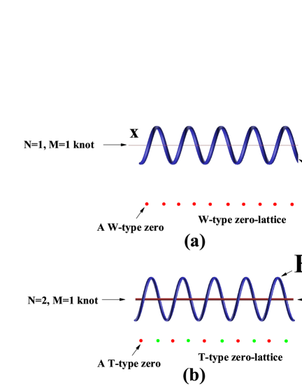
Figure 2: (a) 1D W-type knot (two vortex-lines with winding central axis) and its projected zero-lattice for winding cental axis; (b) 1D T-type knot (two entangled vortex-lines with flat central axis) and its projected zero-lattice between the vortex-lines

To characterize the deformed knot, we project the vortex-membranes $\mathrm{z}(\vec{x},t)=\xi(\vec{x},t)+i\eta(\vec{x},t)$ by solving the zero equation $\hat{P}[\mathrm{z}(\vec{x},t)]\equiv\xi(\vec{x},t)=0.$ After projecting, we show that different entangled vortex-membranes correspond to different zero-lattices. In knot physics, the information is characterized by the distribution of zeroes. Here, the information unit corresponds to a zero between projected vortex-membranes. There exist two types of zero-lattices – T-type zero-lattice and W-type zero-lattice. See the illustration in Fig.2. Firstly, we consider the W-type zero-lattice from projection on a central axis of the two vortex-membranes. A crossing between a helical central axis $\mathrm{z}(\vec{x},t)$ and a straight mathematical membrane ($\mathrm{z}(\vec{x},t)=0$) in its center corresponds to a solution of the equation $\hat{P}_{\theta}[\mathrm{z}(\vec{x},t)]=0,$ that is $\xi(\vec{x},t)=0.$ Next, we consider the T-type zero-lattice from projection on two entangled vortex-membranes themselves. A crossing between the two vortex-membranes ($\mathrm{z}_{\mathrm{A}}(\vec{x},t)$ and $\mathrm{z}_{\mathrm{B}}(\vec{x},t)$) corresponds to a solution of the equation $\hat{P}[\mathrm{z}_{\mathrm{A}}(\vec{x},t)]=\hat{P}[\mathrm{z}_{\mathrm{B}}(\vec{x},t)],$ that is $\xi_{\mathrm{A}}(\vec{x},t)=\xi_{\mathrm{B}}(\vec{x},t).$ According to the existence of two types of zero-lattices, there are two types of zeroes: W-type zero and T-type zero (See Fig.2).

III Emergent quantum mechanics

The elementary excitations of a knot are zeroes with unit information. For a (T-type or W-type) knot, there are three conserved physical quantities: the energy of a (static) zero that is proportional to its volume on vortex-membrane; the (Lamb impulse) angular momentum that is proportional to its volume in the 5D fluid; the winding number $\pm\frac{1}{2}$ or the zero number $\pm 1$. According to the geometric character of the three conserved physical quantities, the shape of zero will never be changed. However, the ”zero” can split and the three physical quantities are conserved for all knot-pieces. Quantum mechanics becomes the mechanics to determine the distribution of knot-pieces.

The five fundamental assumptions of emergent quantum mechanics in knot physics are given by:

1. Quantum states: To characterize the distribution of zeroes, we have introduced the concept of ”knot-pieces”. Quantum mechanics is a mechanics to determine the distribution of knot-pieces, that is the information of a (deformed) knot. Therefore, an important issue is to obtain the spatial and temporal distribution of the knot-pieces that has the information of a (deformed) knot with an extra zero. Quantum state for a particle is just the distribution of zero (or the distribution of knot-pieces for a deformed knot with an extra zero). We point out that the distribution of the knot-pieces and plays the role of the wave-function in quantum mechanics: the angle becomes the quantum phase angle of wave-function and the zero density becomes the density of knot-pieces.

2. Operators: From the point view of information, the momentum denotes the spatial distribution of knot-pieces (or information) and the energy denotes the temporal distribution of knot-pieces (or information). From the point view of fluid mechanics, the momentum is proportional to Lamb impulse and the energy is proportional to the rotating velocity in extra dimensions. As a result, the energy and momentum for the extra zero are described by operators. The effective Planck constant is obtained as projected angular momentum in extra dimensions of the extra knot.

3. Schrödinger equation: The geometric Biot-Savart equation for the deformed knot becomes Schrödinger equation for probability waves of the knot-pieces of a zero. And the classical functions for perturbative Kelvin waves become wave-functions for quantum particle.

4. Fermionic statistics: In quantum mechanics, another assumption is statistics of Fermionic particles. In knot physics, when we exchange two zeroes, the angle in extra dimensions (that is just the phase of wave-function) is $\pi$. As a result, an zero becomes a fermionic particle.

5. Measurement theory: The information is the distribution of zeroes between projected vortex-membranes that is determined by zero density for a given quantum state described by the wave-function. That means to identify the deformation of vortex-membranes, people detect the distribution function of knot-pieces. During measurement processes, the phase angle of knot-pieces is fixed that depends on the time of measurement. This gives an explanation of ”wave-function collapse” in quantum mechanics. The probability of emergent quantum mechanics comes from dynamically detecting the distribution of zeroes, or dynamically projecting entangled vortex-membranes via stochastic projected time under ”fast clock effect” that leads to stochastic projected angle.

In addition, we discuss the complementarity principle and wave–particle duality in knot physics.

In knot physics, complementarity principle comes from complementarity property of knots. On the one hand, a knot-piece is phase-changing – a sharp, time-independent, topological phase-changing; On the other hand, a knot-piece has a fixed phase angle that is determined by wave function. One cannot exactly determine the phase angle of a knot-piece by observing its phase-changing.

Wave-particle duality of quantum particles comes from fragmentation of a unit information in knot physics. On the one hand, a knot is information unit that is a sharp, fragmentized, topological phase-changing and would become a ”point” after projection. Thus, it shows particle-like behavior; On the other hand, the distribution of knot-pieces shows wave-like behavior that is characterized by wave-functions.

IV Emergent gauge theory

Composite knot	Quantum field theory
$\mathcal{N}=1$ and $\mathcal{M}=1$	Weyl Fermion model
$\mathcal{N}=2$ and $\mathcal{M}=1$	Dirac Fermion model
$\mathcal{N}=4$ and $\mathcal{M}=2$	SU(n)*U(1) gauge field theory
$\mathcal{N}=4$ and $\mathcal{M}=3$ with $n=3$	Standard model

Table 1: The correspondence between different quantum field theories in modern physics and the different composite knots in knot physics

We then discuss the Kelvin wave and knot dynamics on complex entangled vortex-membranes – composite knots. By projecting entangled vortex-membranes into several coupled zero-lattices, the information of the system becomes the coupled zero-lattices with internal degrees of freedom. After considering the topological interplay between knots and the internal degrees of freedom (internal twistings, additional internal zeroes) – twist-writhe locking conditionkou3 , different kinds of gauge interactions emerge. In particular, it is the 3D quantum gauge field theories that characterize the knot dynamics of the composite knots. The knot physics may give a complete interpretation on quantum chromodynamics (QCD) and quantum electrodynamics (QED). The collective motions of composite knots are described by quantum fluctuations of zero-lattices: different fermionic elementary particles are zeroes that are topological defects of different zero-lattices with internal-twistings; U(1) gauge field (Maxwell field) are phase fluctuations of internal twistings of internal T-type zero-lattice; SU(N) Yang-Mills field are fluctuations of additional internal zeroes, … Two composite knots interact by exchanging fluctuations of the internal-twistings. In table.1, we show the correspondence between different quantum field theories in modern physics and the different composite knots in knot physics.

A 3D $3$-level composite knot with ($\mathcal{N}=4$, $\mathcal{M}=3$) is an object of 3D four entangled vortex-membranes $\mathrm{A}_{1},$ $\mathrm{A}_{2}$ and $\mathrm{B}_{1},$ $\mathrm{B}_{2}$ in 5D space. Here, $\mathcal{N}$ denotes the number vortex-membranes and $\mathcal{M}$ denotes the number of levels. To generate a $3$-level composite knot with ($\mathcal{N}=4$, $\mathcal{M}=3$), we firstly tangle two symmetric vortex-membranes $\mathrm{A}_{1}$ and $\mathrm{A}_{2}$ and get A-knot. Next, we tangle two symmetric vortex-membranes $\mathrm{B}_{1}$ and $\mathrm{B}_{2}$ and get B-knot. Then, we tangle A-knot and B-knot into a 2-level composite knot with ($\mathcal{N}=4$, $\mathcal{M}=2$). Finally, we symmetrically wind the 2-level knot with ($\mathcal{N}=4$, $\mathcal{M}=2$) along different spatial directions and get a 3D $3$-level composite knot with ($\mathcal{N}=4$, $\mathcal{M}=3$). Fig.3(b) is an illustration of a composite knot with ($\mathcal{N}=4$, $\mathcal{M}=3$). For the $3$-level composite knot, there exist level-1 T/W-type zero-lattices, level-2 T/W-type zero-lattices and level-3 W-type zero-lattices.

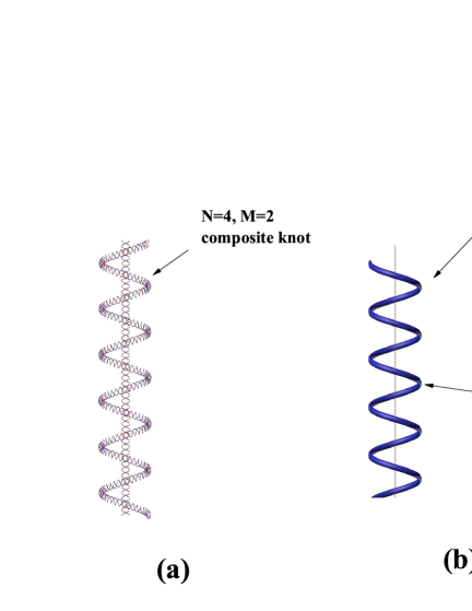
Figure 3: (a) The illustration of 1D $2$-level composite knot with ($\mathcal{N}=4$, $\mathcal{M}=2$); (b) The illustration of 1D $3$-level composite knot with ($\mathcal{N}=4$, $\mathcal{M}=3$). To generate a 1D 3-level composite knot with ($\mathcal{N}=4$, $\mathcal{M}=3$), we symmetrically wind a 1D 2-level knot with ($\mathcal{N}=4$, $\mathcal{M}=2$).

By trapping different types of level-1 internal zeroes, there exist different types of fermionic elementary particles. We use the following number series to label different types of zeroes, $[n_{\mathrm{L}_{2}},$ $n_{\mathrm{L}_{1}}]$ where $n_{\mathrm{L}_{2}}$ is the half linking number of level-2 entangled knot-crystals that is equal to the sum of the number of level-2 T-type zeroes $n_{\mathrm{L}_{2}\mathrm{T}}$ and the number of level-3 W-type zeroes $n_{\mathrm{L}_{3}\mathrm{W}}$ as $n_{\mathrm{L}_{2}}=n_{\mathrm{L}_{2}\mathrm{T}}+n_{\mathrm{L}_{3}\mathrm{W}},n_{\mathrm{L}_{1}}$ is the half linking number of level-1 entangled vortex-membranes that is equal to the sum of the number of level-1 T-type zeroes $n_{\mathrm{L}_{1}\mathrm{T}}$ and the number of level-2 W-type zeroes $n_{\mathrm{L}_{2}\mathrm{W}},$ $n_{\mathrm{L}_{1}}=n_{\mathrm{L}_{1}\mathrm{T}}+n_{\mathrm{L}_{2}\mathrm{W}}.$ For the case of $n=3$, the correspondence between four types of elementary particles is given by

An electron $$\Longleftrightarrow\text{A composite zero with }[1,3]\text{,}$$

A neutrino $$\Longleftrightarrow\text{A composite zero with }[1,0]\text{,}$$

An d-qurak $$\Longleftrightarrow\text{A composite zero with }[1,1]\text{,}$$

An u-qurak $$\Longleftrightarrow\text{A composite zero with }[1,2]\text{.}$$

From point view of fluctuations of level-1 internal twistings, without considering the fluctuations of level-3 W-type windings, the effective model is an $\mathrm{SU_{\mathrm{strong}}(3)}\otimes$U_EM(1) gauge theory. The U(1) gauge symmetry comes from indistinguishable phase of 1-level internal twistings inside a composite zero. Because the exact initial phase of a 1-level internal zero inside a composite zero is not a physical observable value under projection, different choices of initial phase angle of internal twistings lead to same physics result. The U_EM(1) gauge field characterizes the interaction from the phase fluctuations of internal twistings. The SU$\mathrm{{}_{\mathrm{strong}}(}$3) gauge symmetry comes from indistinguishable states of $3$ 1-level internal-zeroes inside the composite knot. The $\mathrm{SU_{\mathrm{strong}}(3)}$ gauge field characterizes the interaction from the fluctuations of additional 1-level internal zeroes. If we set the electric charge for an electron to be $e_{0}$, the electric charge for an internal zero is $\frac{e_{0}}{n}.$ For the case of $n=3$, the charge of an electron with $[1,$ $3]$ is $e_{0};$ the charge of a quark with $[1,$ $2]$ is $\frac{2e_{0}}{3},$ the charge of a quark with $[1,$ $1]$ is $\frac{e_{0}}{3}$, the charge of a neutrino with $[1,$ $0]$ is $0.$ Because electron and neutrino have no additional internal zero, the fluctuations of SU_strong(3) gauge field will never affect electron and neutrino.

After considering the winding fluctuations of level-3 composite knot, the electro-weak $\mathrm{SU}_{\mathrm{weak}}\mathrm{(2)\otimes U}_{\mathrm{Y}}\mathrm{(1)}$ gauge fields emerge. Electro-weak $\mathrm{SU}_{\mathrm{weak}}\mathrm{(2)\otimes U}_{\mathrm{Y}}\mathrm{(1)}$ gauge symmetry comes from the redundancies of 2-level composite zeroes and those of 1-level internal zeroes in unit cell of level-3 W-type zero-lattices. The fluctuations of $\mathrm{SU}_{\mathrm{weak}}\mathrm{(2)}$ gauge theory come from the winding fluctuations of level-3 composite knot and the fluctuations of $\mathrm{U}_{\mathrm{Y}}\mathrm{(1)}$ gauge theory come from the fluctuations of level-1 internal twistings (the internal zeroes) on a unit cell of level-3 W-type zero-lattice. As a result, because the $\mathrm{SU}_{\mathrm{weak}}\mathrm{(2)}$ gauge field characterizes the interaction by exchanging the winding fluctuations of level-3 composite knot, the $\mathrm{SU}_{\mathrm{weak}}\mathrm{(2)}$ gauge fields only couple to the left-handed components of the lepton fields.

The effect of leapfrogging motion is to change a left-hand zero to a right-hand zero. As a result, the fluctuating leapfrogging angular velocity of a Standard knot couples electro-weak $\mathrm{SU}_{\mathrm{weak}}\mathrm{(2)\otimes U}_{\mathrm{Y}}\mathrm{(1)}$ gauge fields and plays the role of Higgs field in Standard model. The finite angular velocity of leapfrogging motion plays the role of Higgs condensation and the Higgs mechanism of 3-level composite knot-crystal with ($\mathcal{N}=4$, $\mathcal{M}=3$) breaks the original gauge symmetry according to $\mathrm{SU}_{\mathrm{weak}}\mathrm{(2)\otimes U}_{\mathrm{Y}}\mathrm{(1)}\rightarrow\mathrm{U}_{\mathrm{EM}}\mathrm{(1)}$.

Finally, we derive the unified theory of Standard knot by considering all points of view. The low energy effective theory is just the Standard model – an $\mathrm{SU_{\mathrm{strong}}(3)}\otimes\mathrm{SU}_{\mathrm{weak}}\mathrm{(2)}\otimes$U_Y(1) gauge theory with Higgs mechanism due to spontaneous symmetry breaking. This is why I call this composite knot with ($\mathcal{N}=4$, $\mathcal{M}=3$) to be the Standard knot.

V Emergent gravity

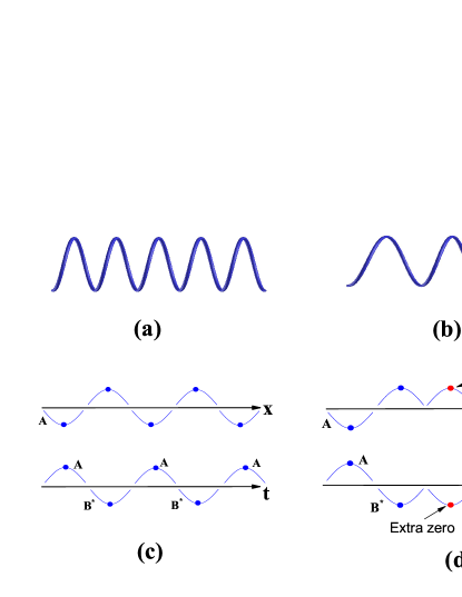
Figure 4: (a) The uniform 1D knot that corresponds to flat space-time for zeroes; (b) The deformed 1D knot that corresponds to curved space-time for zeroes; (c) The illustration of entanglement pattern of a uniform 1D knot with leapfrogging motion; (d) The illustration of entanglement pattern of a 1D leapfrogging knot with an additional zero that is a topological defect.

In knot physics, there exists topological interplay effect between zeroes and the knots: on the one hand, the deformation of the knot leads to the changes of particle motions that can be denoted by curved space-time; on the other hand, the zeroes trapping topological defects deform the knot that indicates matter may curve space-time. The Einstein-Hilbert action becomes a topological mutual BF term that exactly reproduces the low energy physics of the general relativity. We point out that to characterize the entanglement evolution, the corresponding Biot-Savart mechanics for a zero on smoothly deformed knot is mapped to quantum mechanics for particles on a curved space-time. Fig.4(b) is an illustration of deformed 1D knot that corresponds to curved space-time for matter.

For uniform entangled vortex-membranes, the knot is uniform and the scales are (half) winding numbers along spatial/tempo directions. The deformation of the knot leads to deformation of entanglement pattern. In particular, there exists the diffeomorphism invariance that comes from information invariance of zeroes – when the lattice-distance of zero-lattice changes, the size of the zeroes correspondingly changes.

There are two different descriptions to characterize the deformation of the knot. On the one hand, to characterize the changes of the positions of zeroes, we must consider a curved space-time by using geometric description; On the other hand, we can introduce an auxiliary gauge field and use a gauge description to characterize the deformation of the knot. There exists an intrinsic relationship between gauge description for the deformation between two vortex-membranes and geometric description for global coordinate transformation of the same deformed knot.

From point view of geometry, a zero becomes topological defect of the knot – an extra zero is not only anti-phase changing along arbitrary spatial direction but also becomes anti-phase changing along tempo direction. Fig.4(d) is an illustration of 1D deformed knot with an additional knot. From the point view of gauge description, a knot traps a ”magnetic charge” of the auxiliary gauge field. In the path-integral formulation, to enforce such topological constraint, we may add a topological mutual BF term in the action that is just the Einstein-Hilbert action. The variation of the action via the metric gives the Einstein’s equations.

VI Conclusion

In summary, knot physics is developed to understand our universekou1 ; kou2 ; kou3 . The key point of knot physics is the ultimate unification of everything (including matter, motion, interaction and space-time, …) into the entangled vortex-membranes that is a knot, i.e.,

Everything in the universe

$$\iff\text{Entangled vortex-membranes = A knot .}$$

In knot physics, our universe is a projection of Standard knot, a periodic entanglement-pattern between four 3D vortex-membranes. All fundamental interactions are unified into this simple framework, of which the low energy effective theory not only reproduces the Standard model – an $\mathrm{SU_{\mathrm{strong}}(3)}\otimes\mathrm{SU}_{\mathrm{weak}}\mathrm{(2)}\otimes$U_Y(1) gauge theory but also leads to the physics of general relativity. In addition, the new theory yields a deep understanding of the all kinds of elementary particles within different structures of knots.

References

- (1) C. Quigg, Gauge Theories of the Strong, Weak, and Electromagnetc Interactions, Addison–Wesley Pub. Co., Menlo Park, (1983).
- (2) M. Kaku, Introduction to Superstring and M-Theory 2nd edition. New York, Springer-Verlag (1999).
- (3) X.-G. Wen, Quantum Field Theory of Many-Body Systems, (Oxford Univ. Press, Oxford, 2004).
- (4) C. Rovelli, arXiv:1102.3660.
- (5) A. G. Lisi, arXiv:0711.0770 [hep-th] (2007).
- (6) C. Schiller, A fascinating speculation: The strand model.
- (7) R. Penrose, J. Math. Phys. 8, 345 (1967).
- (8) Grigory E. Volovik, The universe in a helium droplet, (Clarendon Press Oxford University Press New York, 2003).
- (9) S. P. Kou, Int. J Mod. Phys. B, V31, 1750241(2017).
- (10) S. P. Kou, Int. J Mod. Phys. B, V32, 1850090 (2018).
- (11) S. P. Kou, arxiv: 1706.06879, to be published as a chapter in book “Superfluids and Superconductors”.
- (12) Boris Khesin, Mosc. Math. J. 12 413 (2012).
- (13) N. Hietala, R. Hänninen, H. Salman, C. F. Barenghi, Phys. Rev. Fluids 1, 084501 (2016).