Linking dissipation-induced instabilities with nonmodal growth: the case of helical magnetorotational instability

Abstract

The helical magnetorotational instability is known to work for resistive rotational flows with comparably steep negative or extremely steep positive shear. The corresponding lower and upper Liu limits of the shear are continuously connected when some axial electrical current is allowed to flow through the rotating fluid. Using a local approximation we demonstrate that the magnetohydrodynamic behavior of this dissipation-induced instability is intimately connected with the nonmodal growth and the pseudospectrum of the underlying purely hydrodynamic problem.

The magnetorotational instability (MRI) VELI is believed to trigger turbulence and enable outward transport of angular momentum in magnetized accretion disks BAHA . The typical Keplerian rotation of the disks belongs to a wider class of flows with decreasing angular velocity and increasing angular momentum, which are Rayleigh-stable RAYLEIGH , but susceptible to the standard version of MRI (SMRI), with a vertical magnetic field $B_{z}$ imposed on the rotating flow. For SMRI to operate, both the rotation period and the Alfvén crossing time have to be shorter than the timescale for magnetic diffusion LIU2006 . For a disk of scale height $H$, this implies that both the magnetic Reynolds number ${\rm Rm}=\mu_{0}\sigma H^{2}\Omega$ and the Lundquist number $S=\mu_{0}\sigma Hv_{A}$ must be larger than one ($\Omega$ is the angular velocity, $\mu_{0}$ the magnetic permeability, $\sigma$ the conductivity, $v_{A}$ the Alfvén velocity).

These conditions are safely fulfilled in well-conducting parts of accretion disks. However, the situation is less clear in the “dead zones” of protoplanetary disks, in stellar interiors, and in the liquid cores of planets, because of low magnetic Prandtl numbers ${\rm Pm}=\nu/\eta$ there BH08 , i.e. the ratio of viscosity $\nu$ to magnetic diffusivity $\eta=(\mu_{0}\sigma)^{-1}$. Moreover, in compact objects like stars and planets even the condition of decreasing angular velocity is not everywhere fulfilled: an important counter-example is the equator-near strip (approximately between $\pm 30^{\circ}$) of the solar tachocline PAME , which is, interestingly, also the region of sunspot activity CHA .

The helical version of MRI (HMRI) is interesting both with respect to the low-${\rm Pm}$ problem as well as for regions with positive shear. Adding an azimuthal magnetic field $B_{\phi}$ to $B_{z}$, Hollerbach and Rüdiger HR95 had shown that this dissipation-induced instability works also in the inductionless limit, ${\rm Pm}=0$, and scales with the Reynolds number ${\rm Re}={\rm Rm}{\rm Pm}^{-1}$ and the Hartmann number ${\rm Ha}=S{\rm Pm}^{-1/2}$, in contrast to SMRI that is governed by ${\rm Rm}$ and $S$. Soon after, Liu et al. LIU showed that HMRI is restricted to rotational flows with negative shear slightly steeper than the Keplerian, or extremely steep positive shear. Specifically, their short-wavelength analysis gave a threshold of the negative steepness of the rotation profile $\Omega(r)$, expressed by the Rossby number ${\rm Ro}=r(2\Omega)^{-1}\partial\Omega/\partial r$, of ${\rm Ro}_{\rm LLL}=2(1{-}\sqrt{2})\approx-0.828$, and a corresponding threshold of the positive shear, at ${\rm Ro}_{\rm ULL}=2(1{+}\sqrt{2})\approx 4.828$. Here, the abbreviations LLL and ULL refer to the lower and upper Liu limits, respectively.

Surprisingly, the same Liu limits were later found APJ12 ; KS1314 to apply also to the so-called azimuthal MRI (AMRI) – a non-axisymmetric ”sibling” of the axisymmetric HMRI that prevails for large ratios of $B_{\phi}$ to $B_{z}$ TEELUCK . Quite recently, the destabilization of steep positive shear profiles by purely azimuthal fields was demonstrated by means of both a short-wavelength analysis SK15 and a one-dimensional stability analysis for a Taylor-Couette flow with narrow gap RUEDIGER .

By allowing axial electrical currents not only at the axis, but also within the fluid, i.e. by enabling the radial profile $B_{\phi}(r)$ to deviate from the current-free case $\propto 1/r$, it was recently shown KS1314 that the LLL and the ULL are just the endpoints of one common instability curve in a plane that is spanned by ${\rm Ro}$ and a corresponding steepness of the azimuthal magnetic field, called magnetic Rossby number, ${\rm Rb}=r(2B_{\phi}/r)^{-1}\partial{(B_{\phi}/r)}/\partial r$. In the limit of large ${\rm Re}$ and ${\rm Ha}$, this curve acquires the closed and simple form

$${\rm Rb}=-\frac{1}{8}\frac{({\rm Ro}+2)^{2}}{{\rm Ro}+1}.$$ (1)

An interesting consequence of this curve is that the strictness of the lower Liu limit ${\rm Ro}_{\rm LLL}=-0.828$, which would prevent Keplerian profiles ${\rm Ro}_{\rm Kep}=-0.75$ from being destabilized by HMRI or AMRI, could be relaxed if only a small amount of the axial current is allowed to pass through the liquid. This effect is now to be investigated in a planned liquid sodium Taylor-Couette experiment DRESDYN , which will combine and enhance the previous experiments on HMRI PRE , AMRI SEIL2 and the kink-type Tayler-instability SEIL1 .

Apart from these interesting theoretical and experimental achievements, the very existence of the two Liu limits (and the shape of their connecting curve Eq. (1) in the ${\rm Ro}-{\rm Rb}$ plane) has remained an unexplained conundrum. This Letter aims at explaining these magnetohydrodynamic features by analysing the dynamics of HMRI from the nonmodal point of view, which has not been done before, and linking them to the nonmodal dynamics of perturbations in the purely hydrodynamic case.

The nonmodal approach to the stability analysis of shear flows in its most general formulation focuses on the finite-time dynamics of perturbations, accounting for transient phenomena due to the shear-induced nonnormality of the flow Trefethen92 ; Farrell1996 ; Schmid_Henningson2001 ; Schmid2007 , in contrast to the canonical modal approach (spectral expansion in time), which is concerned with behavior at asymptotic times. It consists in calculating the optimal initial perturbations with a given positive norm that lead to the maximum possible linear amplification during some finite time. In self-adjoint flow problems, the perturbations that undergo the largest amplification are essentially the most unstable normal modes. By contrast, the situation is nontrivial in non-selfadjoint shear flow problems: the normal mode eigenfunctions are nonorthogonal due to the nonnormality, resulting in transient, or nonmodal growth of perturbations, which can be substantially faster than that of the most unstable normal mode Schmid_Henningson2001 ; Squire2014 . So, leaving the effects of the nonnormality out of consideration and relying only on the results of modal analysis leads to an incomplete picture of the overall dynamics (stability) of shear flows.

Our main goal is to examine the nonmodal dynamics of HMRI in differentially rotating flows, which represent a special class of shear flows for which the nonnormality inevitably plays a role. This can result in growth factors over intermediate (dynamical/orbital) times large compared to the modal growth of HMRI. Recently, the nonmodal dynamics of SMRI was studied by Squire & Bhattacharjee Squire2014 and Mamatsashvili et al. Mamatsashvili2013 ; the present study extends these investigations to the highly resistive, or low-${\rm Pm}$ regime, where only HMRI survives.

We start with the basic equations of nonideal magnetohydrodynamics for incompressible conductive media,

$$\frac{\partial{\bf u}}{\partial t}+{\bf u}\cdot\nabla{\bf u}=-\frac{1}{\rho}\nabla\left(p+\frac{{\bf B}^{2}}{2\mu_{0}}\right)+\frac{{\bf B}\cdot\nabla{\bf B}}{\mu_{0}\rho}+\nu\nabla^{2}{\bf u},$$ (2)

$$\frac{\partial{\bf B}}{\partial t}=\nabla\times\left({\bf u}\times{\bf B}\right)+\eta\nabla^{2}{\bf B},$$ (3)

$$\nabla\cdot{\bf u}=0,~{}~{}~{}\nabla\cdot{\bf B}=0.$$ (4)

where $\rho$ is the constant density, $p$ is the thermal pressure, ${\bf u}$ is the velocity and ${\bf B}$ is the magnetic field.

An equilibrium flow represents a fluid rotating with angular velocity $\Omega(r)$ and threaded by a magnetic field, which comprises a constant axial component $B_{0z}$ and an azimuthal one $B_{0\phi}$ with an arbitrary radial dependence:

$${\bf u}_{0}=r\Omega(r){\bf e}_{\phi},~{}~{}~{}~{}{\bf B}_{0}=B_{0\phi}(r){\bf e}_{\phi}+B_{0z}{\bf e}_{z}.$$

Consider now small axisymmetric ($\partial/\partial\phi=0$) perturbations about the equilibrium, ${\bf u}^{\prime}={\bf u}-{\bf u}_{0}$, $p^{\prime}=p-p_{0}$, ${\bf B}^{\prime}={\bf B}-{\bf B}_{0}$. Following Pessah2005 ; LIU ; KS1314 we adopt a local (WKB) approximation in the radial direction around some fiducial radius $r$, i.e., assume perturbation lengthscales much shorter than the characteristic lengths of radial variations of the equilibrium quantities, and represent perturbations as ${\bf u}^{\prime},{\bf B}^{\prime}\propto\exp({\rm i}k_{r}r+{\rm i}k_{z}z)$, with axial $k_{z}$ and large radial $k_{r}$ wavenumbers, $rk_{r}\gg 1$. Linearizing Eqs. (2)-(4) about the equilibrium and normalizing time by $\Omega^{-1}$, we arrive at the following equations for the perturbations (primes are omitted and the factor $(\mu_{0}\rho)^{-1/2}$ is absorbed in the magnetic field) ${\boldsymbol{\psi}}\equiv(u_{r},u_{\phi},B_{r},B_{\phi}$) (see KS1314 ; Squire2014 for details):

$$\frac{d\boldsymbol{\psi}}{dt}={\bf A}\cdot{\boldsymbol{\psi}},$$ (5)

where the evolution matrix operator ${\bf A}$ is independent of time for axisymmetric perturbations and reads as

$${\bf A}=\begin{pmatrix}-\frac{1}{\rm Re}&2\alpha^{2}&{\rm i}\omega_{z}&-2\omega_{\phi}\alpha^{2}\\ -2(1+{\rm Ro})&-\frac{1}{\rm Re}&2\omega_{\phi}(1+{\rm Rb})&{\rm i}\omega_{z}\\ {\rm i}\omega_{z}&0&-\frac{1}{\rm Rm}&0&\\ -2\omega_{\phi}{\rm Rb}&{\rm i}\omega_{z}&2{\rm Ro}&-\frac{1}{\rm Rm},\end{pmatrix}$$

where $\alpha=k_{z}/k$, $k^{2}=k_{r}^{2}+k_{z}^{2}$, $\omega_{z}\equiv k_{z}B_{0z}/\Omega$ and $\omega_{\phi}\equiv B_{0\phi}/r\Omega$. The Reynolds number, ${\rm Re}=\Omega/\nu k^{2}$, and the magnetic Reynolds number, ${\rm Rm}=\Omega/\eta k^{2}$ are chosen as ${\rm Re}=4000$ and ${\rm Rm}=0.012$, to give a small magnetic Prandlt number ${\rm Pm}={\rm Rm}/{\rm Re}=3\cdot 10^{-6}$ typical for liquid metals and also protoplanetary disks BH08 . The strength of the imposed axial field is measured by the Hartmann number ${\rm Ha}=\omega_{z}\sqrt{{\rm Re}\cdot{\rm Rm}}$, which is fixed to ${\rm Ha}=15$ as typical for liquid metal experiments PRE ; SEIL2 , and the azimuthal field by $\beta=\omega_{\phi}/\omega_{z}$. HMRI is most effective in the presence of an appreciable azimuthal field together with the axial one, $\beta\sim 1$ HR95 ; LIU ; KS1314 . We consider Rayleigh-stable rotation with ${\rm Ro}>-1$ and ${\rm Rb}<0$, since the axial current decreases with radius. It is readily shown that ${\bf A}$ is indeed nonnormal, or non-selfadjoint, i.e., ${\bf A}^{{\dagger}}\cdot{\bf A}-{\bf A}\cdot{\bf A}^{{\dagger}}\neq 0$ and the degree of the nonnormality increases for higher shear ($|{\rm Ro}|$).

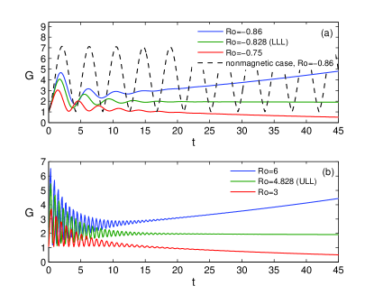
Figure 1: Maximum growth $G(t)$ vs. $t$ at different (a) ${\rm Ro}=-0.86,-0.828({\rm LLL}),-0.75({\rm Kepler})$ and (b) ${\rm Ro}=3,4.828({\rm ULL}),6$. Other parameters are $\alpha=1,Rb=-1$.

Figure 2: $G$ vs. $t$ at different ${\rm Rb}=-1,-0.78,-0.6$ and at fixed (a) ${\rm Ro}_{\rm Kep}=-0.75$ and (b) ${\rm Ro}=3$ both with $\alpha=1$.

We quantify the nonmodal amplification in terms of the total perturbation energy, $E=\frac{\rho}{2}(|{\bf u}|^{2}+|{\bf B}|^{2})={\boldsymbol{\psi}}^{{\dagger}}\cdot F^{{\dagger}}F\cdot{\boldsymbol{\psi}}$, where ${\bf F}=\sqrt{\rho/2}\cdot diag(\alpha^{-1},1,\alpha^{-1},1)$, which is a physically relevant norm. The maximum possible, or optimal growth at a specific time $t$ is defined as the ratio $G(t)=\max_{\boldsymbol{\psi}(0)}E(t)/E(0)$, where $E(t)$ is the energy at $t$ and the maximization is done over all initial states ${\boldsymbol{\psi}}(0)$ with a given initial energy $E(0)$ (e.g., Ref. Schmid_Henningson2001 ). The final state at $t$ is found from the initial state at $t=0$ by solving linear Eq. (5) and can be formally written as ${\boldsymbol{\psi}}(t)={\bf K}(t)\cdot{\boldsymbol{\psi}}(0)$, where ${\bf K}(t)$ is the propagator matrix. Then, the maximum possible amplification $G(t)$ is usually calculated by means of the singular value decomposition technique of ${\bf K}$ (e.g., Refs. Farrell1996 ; Schmid_Henningson2001 ; Trefethen2005 ; Schmid2007 ), which we adopt here. The square of the largest singular value gives the value of $G(t)$ and the corresponding initial condition that achieves this growth (i.e., optimal perturbations) at $t$ is given by the right singular vector of ${\bf K}$. Finally, we would like to stress that studying shear flow stability using the nonmodal approach combined with the method of optimal perturbations is the most general way of analyzing their dynamics at all times, as opposed to the modal approach, which concentrates only on the asymptotic behavior at large times and hence omits an important class of finite-time transient phenomena.

Figure 3: Isolines at $\epsilon=10^{0.25},10^{0.4},10^{0.55},...,10^{3.1}$ show the $\epsilon$-pseudospectra of the ${\bf A}$ matrix in the complex $\omega$-plane for ${\rm Rb}=-1,\alpha=1$ and ${\rm Ro}_{\rm Kep}=-0.75$. The circle indicates the complex $\omega_{K}$ corresponding to the Kreiss constant. The gray curve shows numerical range and the dot on it is the numerical abscissa. Four black dots represent the eigenvalues of the normal modes.

The modal analysis in the WKB approximation yields an expression for the growth rate of HMRI in the relevant limit of small ${\rm Pm}$, but both large ${\rm Re}$ and $\rm Ha$ LIU ; KS1314 . When maximized with respect to $\beta$ (which is typically around unity), this growth rate, given by Eq. (8.30) of KS1314 , becomes (in units of $\Omega$)

$$\gamma=-\frac{{\rm Ha}^{2}}{\rm Re}\left[\frac{({\rm Ro}+2)^{2}}{8(1+{\rm Ro}){\rm Rb}}+1\right],$$ (6)

while the real part of the eigenfrequency is equal to the frequency of inertial waves, $\omega_{\rm iw}=2\alpha\sqrt{1+{\rm Ro}}$. Equation (6) yields the stability boundary Eq. (1) which indicates that for ${\rm Rb}=-1$ the instability (i.e., $\gamma>0$) exists at negative, ${\rm Ro}<{\rm Ro}_{\rm LLL}=-0.828$, and positive, ${\rm Ro}>{\rm Ro}_{\rm ULL}=4.828$, shear, while at larger $-1<{\rm Rb}<0$, the stability region shrinks and the instability extends beyond the Liu limits. As a result, the modal growth of HMRI can also exist for the Keplerian rotation (${\rm Ro}_{\rm Kep.}=-0.75$) starting from ${\rm Rb}=-0.781$ KS1314 .

Now we examine the nonmodal growth of HMRI as a function of time. Figures 1 and 2 show the maximum energy growth $G(t)$ at modally stable and unstable Rossby and magnetic Rossby numbers together with the growth in the modally stable nonmagnetic case, where only the nonmodal growth is possible. In all cases, the initial stage of evolution is qualitatively similar: the energy increases with time, reaches a maximum $G_{m}$ and then decreases. This first nonmodal amplification phase is followed by minor amplifications. Like in the case of modal growth, the kinetic energy dominates over the magnetic one also during nonmodal growth. As a result, the duration of each amplification event is set by inertial waves and is about the half of their period. Correspondingly, the peak value $G_{m}$ is attained at around one quarter of the period, $t_{m}\approx\pi/2\omega_{\rm iw}$, similar to that in the nonmagnetic case, although its value is smaller than that in the latter case. At larger times, the optimal growth follows the behavior of the modal solution – it increases (for ${\rm Ro}=-0.86,6$), stays constant (for the Liu limits, ${\rm Ro}={\rm Ro}_{\rm LLL},{\rm Ro}_{\rm ULL}$) or decays (for ${\rm Ro}=-0.75,3$), respectively, if the flow is modally unstable, neutral or stable; in the latter case HMRI undergoes only transient amplification. This is readily understood: at large times the least stable modal solution (with growth rate given by Eq. 6) dominates, whereas at small and intermediate times the transient growth due the interference of nonorthogonal eigenfunctions is important. In particular, for the Liu limits, where the modal growth is absent, there is moderate nonmodal growth $G_{m}({\rm Ro_{LLL}})=4.06,G_{m}({\rm Ro_{ULL}})=5.46$. A similar evolution of axisymmetric perturbations’ energy with time for HMRI was already found in Priede2007 , where also the physical mechanism of HMRI was explained in terms of an additional coupling between meridional and azimuthal flow perturbations. Importantly, in Fig. 1, $G_{m}$ at modally stable and unstable Rossby numbers are comparable and several times larger than the modal growth factors during the same time $t_{m}$. Indeed, at ${\rm Ro}=-0.86$ the growth achieves the first peak $G_{m}=4.68$ at $t_{m}=1.86$, while at this time the energy of the normal mode would have grown only by a factor of $\exp[2t_{m}\gamma({\rm Ro})]=1.034$. This also implies that in the Keplerian regime, where there is no modal growth of HMRI for ${\rm Rb}=-1$, it still exhibits moderate nonmodal growth (red curves in Figs. 1a and 2a). It is seen from Fig. 2 that the peak $G_{m}$ is almost insensitive to ${\rm Rb}$, however, its effect becomes noticeable as time passes. Decreasing the slope at a given ${\rm Ro}$ increases the optimal growth and at large times makes the flow modally unstable.

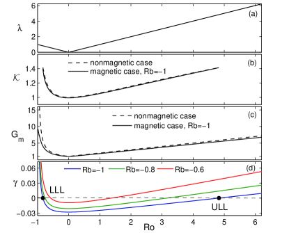
Figure 4: (a) numerical abscissa, $\lambda$, (b) Kreiss constant, ${\cal K}$ (c) $G_{m}$ for HMRI at ${\rm Rb}=-1$ as well as in the nonmagnetic case and (d) modal growth rate of HMRI from Eq. (6) vs. ${\rm Ro}$ at different ${\rm Rb}=-1,-0.8,-0.6$ and $\alpha=1$.

The other relevant notions used to characterize the nonmodal growth and its connection with the results of modal analysis are the pseudospectra and numerical range of the nonnormal operator ${\bf A}$ Schmid_Henningson2001 ; Trefethen2005 ; Schmid2007 . The maximal protrusion of the numerical range into the upper (unstable) half in the complex $\omega$-plane – a numerical abscissa, $\lambda$, defines the maximum growth rate at the beginning of evolution (at $t=0^{+}$), $2\lambda=\max_{{\boldsymbol{\psi}}(0)}E(t)^{-1}dE(t)/dt|_{t=0^{+}}$. On the other hand, the extent to which the pseudospectra contours penetrate into the upper half of the $\omega$-plane determines the amount of transient amplification over time. This is quantified by the Kreiss constant ${\cal K}=\max_{{\rm Im}(\omega)>0}{\rm Im(\omega)}||({\bf A}+{\rm i}\omega{\bf I})^{-1}||$, where ${\bf I}$ is the unit matrix and $||\cdot||$ denotes a suitably defined norm Schmid_Henningson2001 ; Trefethen2005 . This constant provides a lower estimate for the maximum nonmodal amplification of energy over time, i.e., $\max_{t>0}G(t)\geq{\cal K}^{2}$ Schmid_Henningson2001 ; Schmid2007 .

Figure 3 shows the normal mode spectra of Eq. (5) and the associated pseudospectra in the $\omega$-plane at ${\rm Ro}_{\rm Kep}=-0.75$, where all the eigenfrequencies (thick black dots) are in the lower half plane, indicating modal stability against HMRI. The mode which is closer to the ${\rm Im}(\omega)=0$-axis will first cross it and exhibit HMRI as ${\rm Ro}$ changes beyond the Liu limits, while the other two modes far in the lower half plane are rapidly damped magnetic (SMRI) modes. On the other hand, the numerical abscissa and the frequency, $\omega_{K}$, that results in the Kreiss constant, lie in the upper plane, which indicates the nonmodal amplification larger than ${\cal K}^{2}$ takes place over intermediate times.

Figure 4, which illustrates the central result of this Letter, shows (a) the numerical abscissa $\lambda$, (b) the Kreiss constant ${\cal K}$, (c) the maximum growth $G_{m}$ for ${\rm Rb}=-1$ and in the nonmagnetic case as well as (d) the modal growth rate $\gamma$ given by Eq. (6) at ${\rm Rb}=-1,-0.8,-0.6$ versus ${\rm Ro}$. The numerical abscissa, measuring the initial optimal growth rate of the energy, is equal to $|{\rm Ro}|$, i.e., to the maximum growth rate of ideal SMRI (see also Ref. Squire2014 ) despite the very high resistivity of the flow. $G_{m}$ increases linearly with ${\rm Ro}$ at ${\rm Ro}>0$ and much steeper at ${\rm Ro}<0$ which can be well approximated by $\propto(1+{\rm Ro})^{-0.78}$. For comparison, in this plot we also show the maximum transient growth factor for axisymmetric perturbations in the nonmagnetic case, $G_{m}^{(h)}=(1+{\rm Ro})^{{\rm sgn}({\rm Ro})}$, as derived in Afshordi2005 . So, although $G_{m}$ in the magnetic case is slightly smaller than that in the nonmagnetic one, the two curves are in fact close to each other and display nearly the same behavior with ${\rm Ro}$, a feature that is also shared by the Kreiss constant (b). Note that the dependencies of $G_{m}$, $G_{m}^{(h)}$ (Fig. 4c) and of the modal growth rate $\gamma$ (Fig. 4d) on ${\rm Ro}$ have very similar shapes. Remarkably, the latter, being given by Eq. (6), can be expressed in terms of the hydrodynamic nonmodal growth $G_{m}^{(h)}=(1+{\rm Ro})^{{\rm sgn}({\rm Ro})}$ in the closed form (${\rm Rb}=-1$)

$$\gamma=\frac{{\rm Ha}^{2}}{\rm Re}\left[\frac{(G_{m}^{(h)}+1)^{2}}{8G_{m}^{(h)}}-1\right]$$ (7)

which is indeed proportional to $G_{m}^{(h)}$ for larger values. Both Liu limits, at which HMRI sets in, are therefore connected with a corresponding threshold $G_{m}^{(h)}({\rm Ro}_{\rm LLL})=G_{m}^{(h)}({\rm Ro}_{\rm ULL})=5.828$.

In this Letter, we have investigated the nonmodal dynamics of HMRI due to the nonnormality of a magnetized shear flow with large resistivity. We traced the entire time evolution of the optimal growth of the perturbation energy and demonstrated how the nonmodal growth stage smoothly carries over to the modal behavior at large times. At small and intermediate (orbital/dynamical) times, HMRI undergoes transient amplification with the initial growth rate being equal to that of the most unstable SMRI. Then, it reaches a maximum, which is higher for larger $|{\rm Ro}|$, and finally at asymptotic times, it decays or increases exponentially, respectively, when ${\rm Ro}$ lies within or beyond the Liu limits. The transient growth of HMRI is generally several times larger than its modal growth during the dynamical time. It also occurs in the Keplerian regime, where the modal HMRI is thought to be non-existing. As illustrated in Fig. 4, and quantified exactly in Eq. (7), the modal growth rate of HMRI displays quite a similar dependence on ${\rm Ro}$ as the maximum nonmodal growth in the purely hydrodynamic shear flow, which indicates a fundamental connection between nonmodal dynamics and dissipation-induced modal instabilities, such as HMRI. Both, despite the latter being magnetically triggered, rely on hydrodynamic means of amplification, i.e., they extract energy from the background flow mainly by Reynolds stress due to shear Priede2007 .

This work was supported by the Alexander von Humboldt Foundation and the German Helmholtz Association in frame of the Helmholtz Alliance LIMTECH.

References

- (1) E.P. Velikhov, JETP 9, 995 (1959).
- (2) S.A. Balbus, J.F. Hawley, Rev. Mod. Phys. 70, 1 (1998).
- (3) Lord Rayleigh, Proc. R. Soc. London A 93, 148 (1917).
- (4) W. Liu, J. Goodman, H. Ji, Astrophys. J. 643, 306 (2006)
- (5) S.A. Balbus, P. Henri, Astrophys. J. 674, 408 (2008)
- (6) K.P. Parfrey, K. Menou, Astrophys. J. Lett. 667, L207 (2007)
- (7) P. Charbonneau, Liv. Rev. Sol. Phys. 7, 3 (2010)
- (8) R. Hollerbach, G. Rüdiger, Phys. Rev. Lett. 95, 124501 (2005)
- (9) W. Liu, J. Goodman, I. Herron, H. Ji, Phys. Rev. E 74, 056302 (2006)
- (10) O. Kirillov, F. Stefani, Astrophys. J., 712, 52 (2010); O.N. Kirillov, F. Stefani, Y. Fukumoto, Astrophys. J. 756, 83 (2012); O. Kirillov, F. Stefani, Phys. Rev. Lett. 111, 061103 (2013)
- (11) O. Kirillov, F. Stefani, Y. Fukumoto, J. Fluid Mech. 760, 591 (2014)
- (12) R. Hollerbach, V. Teeluck, G. Rüdiger, Phys. Rev. Lett. 104, 044502 (2010)
- (13) F. Stefani, O. Kirillov, Phys. Rev E 92, 051001(R) (2015)
- (14) G. Rüdiger et al. Phys. Fluids 28, 014105 (2016).
- (15) F. Stefani et al., Magnetohydrodynamics, 48, 103 (2012)
- (16) F.Stefani et al., Phys. Rev. Lett. 97, 184502 (2006); F. Stefani et al., Phys. Rev. E. 80, 066303 (2009)
- (17) M. Seilmayer et al., Phys. Rev. Lett. 113, 024505 (2014)
- (18) M. Seilmayer et al., Phys. Rev. Lett. 108, 244501 (2012)
- (19) L. Trefethen, A. Trefethen, S. Reddy, T. Driscoll, Science, 261, 578 (1993)
- (20) B. Farrell, P. Ioannou, J. Atmos. Sci. 53, 2025 (1996)
- (21) P. Schmid, D. Henningson, Stability and Transition in Shear Flows (Springer Verlag, New York, 2001)
- (22) P. Schmid, Annu. Rev. Fluid Mech., 39, 129 (2007)
- (23) J. Squire, A. Bhattacharjee, Phys. Rev. Lett., 113, 025006 (2014); J. Squire, A. Bhattacharjee, Astrophys. J., 797, 67 (2014)
- (24) G. Mamatsashvili, G. Chagelishvili, G. Bodo, P. Rossi, Mon. Not. R. Astron. Soc., 435, 2552 (2013)
- (25) L. Trefethen, M. Embree, Spectra and Pseudospectra, The behavior of Nonnormal Matrices and Operators (Princeton University Press, Princeton, NJ, 2005)
- (26) M. Pessah, D. Psaltis, Astrophys. J., 628, 879 (2005)
- (27) J. Priede, I. Grants, G. Gerbeth, Phys. Rev. E, 75, 047303 (2007)
- (28) N. Afshordi, P. Mukhopadhyay, R. Narayan, Astrophys. J., 629, 373 (2005)