Dynamically flavored description of holographic QCD in the presence of a magnetic field

Abstract

We construct the gravitational solution of the Witten-Sakai-Sugimoto model by introducing a magnetic field on the flavor brane. With taking into account their backreaction, we re-solve the type IIA supergravity in the presence of the magnetic field. Our calculation shows the gravitational solutions are magnetic-dependent and analytic both in the bubble (confined) and black brane (deconfined) case. We study the dual field theory at the leading order in the ratio of the number of flavors and colors, also in the Veneziano limit. Some physical properties related to the hadronic physics in an external magnetic field are discussed by using our confined backreaction solution holographically. We also investigate the thermodynamics and holographic renormalization of this model in both phases by our solution. Since the backreaction of the magnetic field is considered in our gravitational solution, it allows us to study the Hawking-Page transition with flavors and colors of this model in the presence of the magnetic field. Finally we therefore obtain the holographic phase diagram with the contributions from the flavors and the magnetic field. Our holographic phase diagram is in agreement with lattice QCD result qualitatively, which thus can be interpreted as the inhibition of confinement or chirally broken symmetry by the magnetic field.

Si-wen Li and Tuo Jia

1 Introduction

Motivation

Recent years, in some results from lattice QCD [1, 2], it seems the QCD phase could be changed by a strong magnetic field. By the analysis of some thermodynamic observables, it has been found the critical temperature of the crossover region should fall when the magnetic field increases [1, 2]. It implies the confinement/deconfinement phase transition or the chiral phase transition [3] would tend to be induced by a strong magnetic field. With the MIT bag model, this result could be reproduced qualitatively [4], reflecting the great significance of quark confinement. Furthermore, the approach of large-$N_{c}$ QCD has already been considered in [5]. From the analysis of the flavor correction $N_{f}/N_{c}$ to the pressure, this effect has also been obtained due to the quark degrees of freedom. On the other hand, gauge/gravity duality or AdS/CFT has become a framework to understand non-perturbative aspects of strong-coupled quantum field theory [6, 7, 8]. Therefore, the motivation of our work is to investigate the thermodynamics of the quarks and gluons by using the holographic method in the presence of a magnetic field with considering the dynamics of the flavors.

Model

The famous Witten-Sakai-Sugimoto model [9, 10] is the model which currently becomes closest to QCD since it has been proposed to holographically study the non-perturbative QCD for a long time, for examples [11, 12, 13, 14, 15, 16, 17, 18, 19, 20, 21]. By the underlying string theory, this model describes a non-supersymmetric and non-conformal Yang-Mills theory in 3+1 dimension coupled to $N_{f}$ chiral massless fermions (quarks) and adjoint massive matter, as a low energy effective theory. In this model, there are $N_{c}$ D4-branes compactified on a circle representing the dynamics of gluons, $N_{f}$ species of massless quarks introduced by putting in $N_{f}$ pairs of D8 and anti D8-branes ($\overline{\mathrm{D8}}$-branes). By taking the large $N_{c}$ limit i.e. $N_{f}\ll N_{c}\rightarrow\infty$, these $N_{c}$ D4-branes produce a 10D background geometry described by type IIA supergravity while the $N_{f}$ $\mathrm{D}8/\overline{\mathrm{D}8}$-branes are as probes. Accordingly, the fundamental quarks do not have dynamical degrees of freedoms thus they are quenched.

Furthermore, the description of deconfinement transition and chiral transition in the Witten-Sakai-Sugimoto model was proposed in [11]. At zero temperature, the bubble (confined) solution of the $N_{c}$ D4-branes is dominant, corresponding the confinement phase in the dual field theory, while the black brane (deconfined) solution of the $N_{c}$ D4-branes arises as the deconfinement phase at high temperature. Thus the phase transition between confinement and deconfinement can be identified as the Hawking-Page transition between two different background geometries. We can therefore evaluate the critical temperature by the analysis of the pressure in bubble and black brane background. The result shows that a confinement/deconfinement transition at $T_{c}=M_{KK}/2\pi$ arises, where $M_{KK}$ is a mass scale of the mass spectrum. However, while the bubble solution can be connected to the confinement phase of the dual field theory, this is less clear for the black brane solution because of the mismatched value of the Polyakov loops [17, 22, 23], which thus makes “the black D4-brane solution corresponding the deconfinement phase” may not be strictly rigorous. Nevertheless, we can focus on the chiral transition in this setup since the embedded flavor branes take connected/parallel configuration in the bubble/black D4-brane solution respectively, which corresponds to the chirally broken/symmetric phase in the dual field theory.

Goal and method

Our goals for this paper are collected as follows,

1. Construct gravitational solutions of this model by taking account of the backreaction from the flavor brane with a magnetic field. Then investigate some physical quantities in confinement phase with our solution.

2. Study the holographic renormalization, thermodynamics and Hawking-Page transition with our gravitational solutions. Compare our results with lattice QCD [1, 2].

In order to achieve the goals above, let us outline some technical details in our manuscript. First, we use the smearing technique [24, 25, 26, 27, 28] for the flavor branes to construct gravitational solutions as [18] in the presence of a magnetic field (with zero chemical potential). Then in order to preserve the isometries of the original background, we also homogeneously smear a large number $N_{f}$ of D8-branes on the $x_{4}$ circle where the $N_{c}$ D4-branes are wrapped. As it will be seen, while this configuration simplifies the calculations greatly, we have to solve a set of coupled second order equations of motion of this system. Because of the presence of the magnetic field, these equations of motion are all highly non-linear which are still extremely complicated to solve. Hence we focus on solving these equations in the limit of small magnetic field and small flavor backreaction since it admits analytically magnetic-dependent solutions. To determine the integration constants in our solution, we furthermore require that the backgrounds must be completely regular in the IR region of the dual field theory. With the presence of the magnetic field, the integration constants could be able to depend on the constant magnetic field. However, we find it is not enough to determine all the integration constants just by these geometric requirements. Besides, in the UV region, there also is an non-removable divergence unaffected by the presence of the magnetic field, which is due to the Landau pole in field theory, reflecting in the running coupling holographically.

Last but not least, since the onshell action evaluated by our gravitational solutions is divergent, we need to holographically renormalize the theory in order to study its thermodynamics. The counterterms have been computed with a magnetic field and we find if the parameters in the covariant counterterms depend on the magnetic field, they are enough to cancel all the divergences in our calculations. Then we can obtain the phase diagram by comparing the renormalized confined/deconfined pressure. Our holographic phase diagram shows, the critical temperature decreases when the magnetic field increases in the probe approximation, which qualitatively agrees with the lattice QCD results [1, 2].

Relation to previous works and outline

The thermodynamics of holographic QCD with this model has been widely studied in many present works [11, 15, 16, 17, 19, 20, 21, 29], however the backreaction case is not considered in these works. Particularly, in [18], the dynamical flavors have been taken into account in this model without magnetic field. In [29], the thermodynamics of the quarks and gluons in the presence of a magnetic field has been studied (without the flavored backreaction). Thus we would like to combine [18] with [29] in this manuscript. Technically, our calculation is an extension of [18] by introducing the dependence of the magnetic field, so we will employ the similar conventions as in [18].

This paper is organized as follows. In the next Section 2, we will give a brief review of the Witten-Sakai-Sugimoto model. In Section 3, we introduce a magnetic field on the flavor brane and construct the gravitational solution by re-solving the type IIA plus flavor brane action, both in confined (bubble) case and deconfined (black brane) case. The magnetic-dependent solution is also given in this section. In Section 4, we discuss some physical quantities by imposing the constructed solution with some special constraints in the confined case. In section 5, it shows the holographic renormalization in our calculation, then we evaluate the renormalized onshell action and the counterterms by our magnetic-dependent solutions. In Section 6, we discuss the holographic phase diagram with the magnetic field in the case of the probe approximation and backreaction respectively, then compare our results with lattice QCD. Discussion and summary are given in the final section.

2 Reviews of the Witten-Sakai-Sugimoto model

In this section, we review the Witten-Sakai-Sugimoto model systematically.

A non-supersymmetric and non-conformal (3+1 dimensional) Yang-Mills theory was proposed by Witten [34] as the low energy limit of a Kaluza-Klein (KK) reduction of a 5+1 dimensional $SU\left(N_{c}\right)$ super conformal theory which couples to massless adjoint scalar and fermions. This theory is the low energy effective theory describing the open string ending on the worldvolume of $N_{c}$ coincident D4-branes placed in the 10D Minkowskian spacetime. By the dimensional reduction, the theory is compactified on a circle (denoted as $x_{4}$) of length $\beta_{4}$. With the choice of boundary conditions for bosons (periodic b.c.) and fermions (anti-periodic b.c.), the massless modes at low energy scale i.e. $E\ll 1/\beta_{4}$ are the gauge fields of 3+1 dimensional $SU(N_{c})$ Yang-Mills theory. The supersymmetry breaks down since the other modes (including fermions) get masses $M_{kk}\sim 1/\beta_{4}$. If $T_{s}/M_{KK}=2\lambda_{4}/27\pi\ll 1$, where $T_{s},\ \lambda_{4}$ is the string tension and 4d ’t Hooft coupling respectively, the low energy theory could be decoupled from the Kaluza-Klein modes.

However, as it is known there is not any simple description in the most interesting region $\lambda_{4}\sim 1$ in Witten’s model. As a conjecture by holography, there should be a dual description in terms of a classical gravity theory on a background arising as the near-horizon limit of sourced $N_{c}$ D4-branes, we can therefore obtain many detailed informations in the region of $\lambda_{4}\gg 1$. Such a background produced by $N_{c}$ D4-branes would have the topology of a product $\mathbb{R}^{1,3}\times\mathbb{R}_{u}\times S_{x_{4}}\times S^{4}$. Here $\mathbb{R}^{1,3}$ represents the 3+1 dimensional spacetime where we live in. $\mathbb{R}_{u}$ represents the radial direction denoted by the coordinate $u$ as the holographic direction, which could be roughly treated as the energy scale of the renormalization group in the dual field theory. In the $\left(u,\ x_{4}\right)$ plane of the subspace, the confined background looks like a cigar and the size of the $x_{4}$ circle smoothly shrinks to zero at a finite value $u_{KK}$ of the radial coordinate $u$. $S^{4}$ represents the additional dimensions, whose isometry group is $SO\left(5\right)$ identified as a global symmetry group under rotation of the massive Kaluza-Klein fields. The theory describes confinement in the dual field theory and the chiral symmetry breaks at zero temperature once it couples to the chiral massless quarks.

It is achieved to add a stack of $N_{f}$ pairs of suitably $\mathrm{D}8/\overline{\mathrm{D}8}$-branes embedded in the $N_{c}$ D4-branes background geometry to introduce $N_{f}$ chiral fundamental massless quarks as [9] in Witten’s model. Quarks are in the fundamental representation of color and flavor group since they come from the massless spectrum of the open strings which are stretching between the color and flavor branes. Because the flavor $\mathrm{D}8/\overline{\mathrm{D}8}$-branes are probes in this system, their backreaction to the geometric background is neglected. Correspondingly, the fundamental quarks in the dual field theory are in the quenched approximation. Besides, the flavor branes offer a $U_{R}\left(N_{f}\right)\times U_{L}\left(N_{f}\right)$ symmetry which could be identified as the global flavor symmetry holographically. Then it is recognized that the flavor branes connect to each other as a U-shape at zero temperature representing chirally broken symmetry automatically.

In the bubble (confined) background, the geometry is described by the bubble solution of $N_{c}$ D4-brane with the following metric,

$$ds^{2} =\ \left(\frac{u}{R}\right)^{3/2}\left[\eta_{\mu\nu}dx^{\mu}dx^{\nu}+f\left(u\right)dx_{4}^{2}\right]+\left(\frac{R}{u}\right)^{3/2}\left[\frac{du^{2}}{f\left(u\right)}+u^{2}d\Omega_{4}^{2}\right]$$

$$e^{\phi} =\ g_{s}\left(\frac{u}{R}\right)^{3/4},\ \ \ F_{4}=\frac{3N_{c}}{4\pi}\omega_{4},\ \ \ f\left(u\right)=1-\frac{u_{KK}^{3}}{u^{3}}.$$ (2.1)

where $R^{3}=\pi g_{s}N_{c}l_{s}^{3}$ is the curvature radius of the background geometry and $\omega_{4}$ is the volume form of $S^{4}$, $g_{s}$ and $l_{s}$ is the string coupling and length respectively. $\phi$ is dilaton and $F_{4}$ is the Ramond-Ramond four form. For the index, we have defined $\mu=0,1,2,3$. At the scale $M_{KK}$, the ’t Hooft coupling is defined as $\lambda_{4}=g_{YM}^{2}N_{c}=4\pi^{2}g_{s}N_{c}l_{s}/\beta_{4}$ in the 4-dimensional theory. Since $f\left(u_{KK}\right)=0$, the $x_{4}$ circle shrinks at $u=u_{KK}$. In order to omit the conical singularities at $u=u_{KK}$, it provides the following relation,

$$9\beta_{4}^{2}u_{KK}=16\pi^{2}R^{3}.$$ (2.2)

Here $\beta_{4}$, as the length of the $x_{4}$ circle, is related to the mass scale $M_{KK}$ by $\beta_{4}=2\pi/M_{KK}$.

There is an alternatively allowed solution which is the black brane (deconfined) solution taking the following metric,

$$ds^{2} =\ \left(\frac{u}{R}\right)^{3/2}\left[-f_{T}\left(u\right)dt^{2}+\delta_{ij}dx^{i}dx^{j}+dx_{4}^{2}\right]+\left(\frac{R}{u}\right)^{3/2}\left[\frac{du^{2}}{f_{T}\left(u\right)}+u^{2}d\Omega_{4}^{2}\right]$$

$$f_{T}\left(u\right) =\ 1-\frac{u_{T}^{3}}{u^{3}}.$$ (2.3)

Here $i,j=1,2,3$. Similarly, it provides the following relation with the $x_{0}$ circle smoothly shrinking to zero at the horizon $u=u_{T}$,

$$9\beta^{2}u_{T}=16\pi^{2}R^{3}.$$ (2.4)

Therefore, we have the Hawking temperature as

$$T=1/\beta,$$ (2.5)

where $\beta$ is the length of $x^{0}$ in the deconfined geometry.

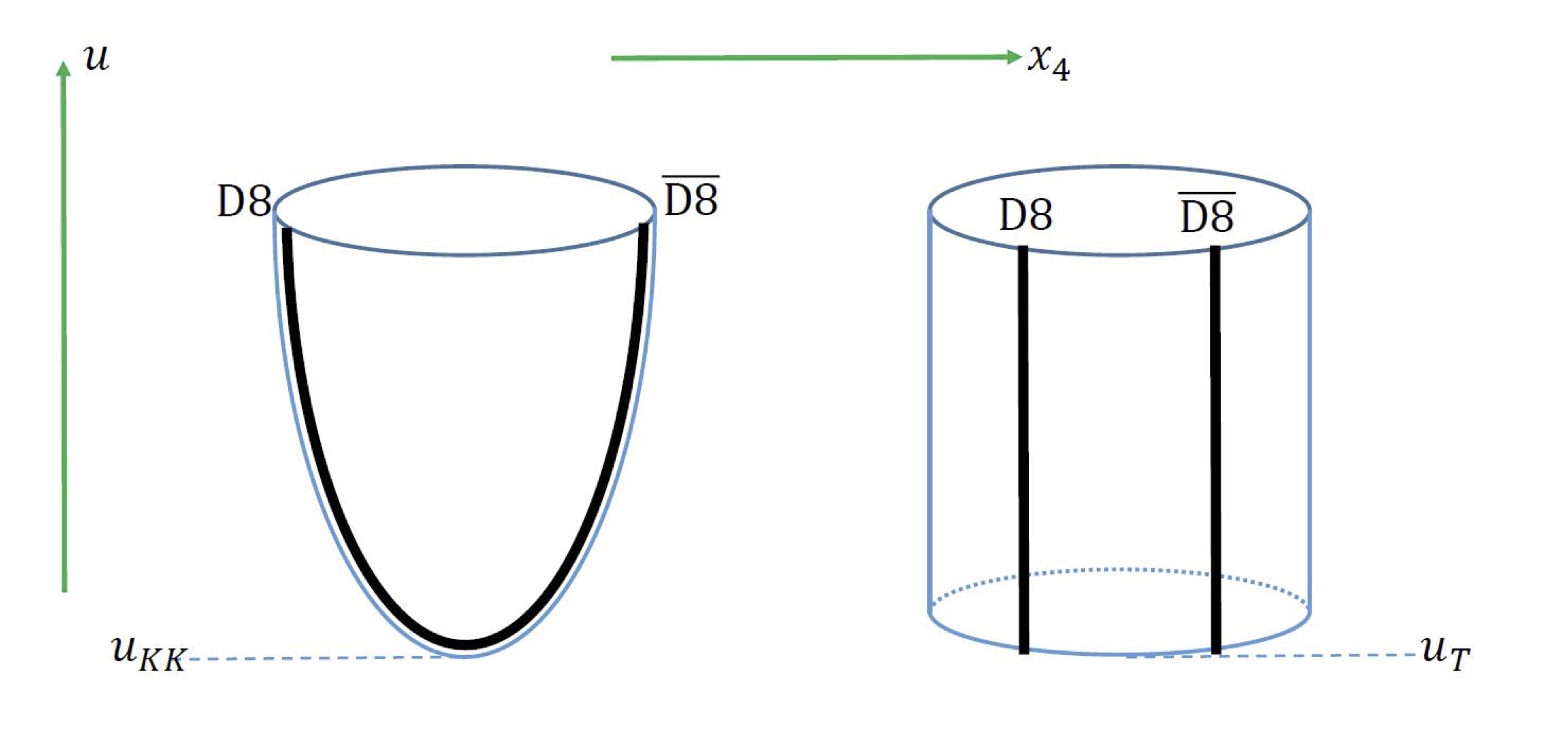
Figure 1: Phase Transition in our model. Left: In confined geometry the flavor $\mathrm{D}8/\overline{\mathrm{D}8}$-branes are located at antipodal points of $x_{4}$ - circle and always connected, realizing as chirally broken phase. Right: In deconfined geometry the flavor $\mathrm{D}8/\overline{\mathrm{D}8}$-branes could be parallel, realizing as chirally symmetric phase.

In the classical limit, the gravity partition function $Z\sim e^{-S}$, which is related to the Euclidean onshell action, could be identified as the free energy of the system thermodynamically. The phase diagram can be obtained by comparing the free energy of the two phases above. It has turned out the bubble solution is dominant at zero temperature, while the black brane solution of the $N_{c}$ D4-branes arises at high temperature, which provides the critical temperature of the phase transition as,

$$T_{c}=1/\beta_{4}=\frac{M_{KK}}{2\pi}.$$ (2.6)

In this manuscript, we are going to work in the following configuration when the flavor branes are considered. That is, in the confined case, the $\mathrm{D}8/\overline{\mathrm{D}8}$-branes are placed at antipodal points of $x_{4}$ - circle. When the temperature increases, the connected position on $\mathrm{D}8/\overline{\mathrm{D}8}$-branes falls into the horizon in the $T>T_{c}$ phase as in Figure 1. It thus turns to the deconfined case and the $\mathrm{D}8/\overline{\mathrm{D}8}$-branes become parallel (disconnected). Accordingly, the chiral symmetry is restored since the flavor symmetry group remains $U_{R}\left(N_{f}\right)\times U_{L}\left(N_{f}\right)$ in the configuration of a stake of parallel $\mathrm{D}8/\overline{\mathrm{D}8}$-branes. So the confined/deconfined or chiral phase transition could be identified as the Hawking-Page transition of the background with the connected/parallel configuration of the flavor branes.

3 Solutions with the flavored backreaction in the presence of a magnetic field

In the following sections, there would be three relevant and useful coordinates which are $\rho,\ x,\ r$. For the reader convenience, the relation of these coordinates and the standard $u$ coordinate used in the Witten-Sakai-Sugimoto model (2.1) (2.3) is summarized as follows,

$$e^{-3r}=1-\frac{u_{0}^{3}}{u^{3}},\ r=a\rho,\ x=e^{-3r/2}.$$ (3.1)

As it will be seen that $u_{0}$ represents $u_{KK}$ in confined geometry or $u_{T}$ in deconfined geometry. We are going to use $a_{T}$ to replace $a$ in (3.1) in the deconfined geometry and the explicit definition of $a$ or $a_{T}$ could be found in the following relevant formulas (in Eq.(3.13) and Eq.(3.32)). Since our calculation is an extension of [18], we will employ the similar conventions as in [18].

3.1 Confined geometry

Ansatz and solution

In the Witten-Sakai-Sugimoto model [9], the flavor $\mathrm{D}8/\overline{\mathrm{D}8}$-branes are treated as the probes embedded in the confined geometry. However, in this subsection we would like to take into account their backreaction to the first order of $N_{f}/N_{c}$ in the confined case. Hence we are going to use the same trick as [18], that is to consider a setup where $N_{f}$ D8-branes are smeared homogeneously along the transverse $x_{4}$ circle [24, 25, 26, 27, 28]. And we will consider the model below the critical temperature ($T<T_{c}$) with a background magnetic field on the flavor branes.

For $T=0$, the ansatz of the metric in string frame is given as [11],

$$ds^{2}=e^{2\lambda}\left(-dt^{2}+dx_{a}dx^{a}\right)+e^{2\tilde{\lambda}}dx_{4}^{2}+l_{s}^{2}e^{-2\varphi}d\rho^{2}+l_{s}^{2}e^{2\nu}d\Omega_{4}^{2},$$ (3.2)

where $a=1,2,3$ and $\lambda,\tilde{\lambda},\nu,\phi$ are functions depended on the holographic coordinate $\rho$ only. $x_{4}$ is the compactified coordinate on a circle with the length $\beta_{4}=2\pi/M_{KK}$. The function $\varphi$ are defined as

$$\varphi=2\phi-4\lambda-\tilde{\lambda}-4\nu.$$ (3.3)

In order to take into account the backreaction of the flavor and the magnetic field, we have to consider the total action in type IIA supergravity with the presence of a magnetic field on the flavor branes. The relevant action (bulk fields plus smeared flavor brane) is,

$$S =\frac{1}{2k_{0}^{2}}\int d^{10}x\sqrt{-g}\left[e^{-2\phi}\left(\mathcal{R}+4\left(\partial\phi\right)^{2}\right)-\frac{1}{2}\left|F_{4}\right|^{2}\right]$$

$$\ \ -\frac{N_{f}T_{8}M_{KK}}{\pi}\int d^{10}x\frac{\sqrt{-\det\left(g+2\pi\alpha^{\prime}F\right)}}{\sqrt{g_{44}}}e^{-\phi}.$$ (3.4)

The first part of (3.4) is the action of the bulk fields while the last part arises as the contribution from the Dirac-Born-Infield (DBI) action of $N_{f}$ D8-branes which are smeared on the transverse $x_{4}$ circle. Here $k_{0}$ is related to the 10d Newton coupling. In confined geometry, we consider the antipodal configuration for the flavor branes and put the smeared DBI action on-shell i.e. the embedding coordinate $x_{4}=x_{4}\left(\rho\right)$ satisfies its equation of motion $\frac{d}{d\rho}x_{4}=0$. The integration over the radial coordinate has been calculated as two times to account for the presence of two branches at two antipodal points on the $x_{4}$. Furthermore, we have turned on a $U\left(1\right)$ gauge field on the flavor branes which is the dual of an external background magnetic field. Thus as [19, 29, 30] we set a constant magnetic field $2\pi\alpha^{\prime}F_{12}=b$, where $b$ is dimensionless constant. With the implementation of the ansatz (3.2), it yields the following 1d action [11, 18],

$$S = \mathcal{V}\int d\rho\left[-4\dot{\lambda}^{2}-\dot{\widetilde{\lambda}}^{2}-4\dot{\nu}^{2}+\dot{\varphi}^{2}+V+\mathrm{total\ derivatives}\right],$$

$$V = 12e^{-2\nu-2\varphi}-Q_{c}^{2}e^{4\lambda+\widetilde{\lambda}-4\nu-\varphi}-Q_{f}e^{2\lambda-\frac{\widetilde{\lambda}}{2}+2\nu-\frac{3}{2}\varphi}\sqrt{1+b^{2}e^{-4\lambda}},$$ (3.5)

where we have defined

$$R^{3} =\pi g_{s}N_{c}l_{s}^{3},\ \ Q_{c}=\frac{3}{\sqrt{2}g_{s}}\frac{R^{3}}{l_{s}^{3}}=\frac{3\pi N_{c}}{\sqrt{2}},\ \ \epsilon_{f}=\frac{R^{3/2}u_{0}^{1/2}g_{s}}{l_{s}^{2}}Q_{f},$$

$$Q_{f} =\frac{2k_{0}^{2}N_{f}T_{8}M_{KK}l_{s}^{2}}{\pi},\ \ \mathcal{V}=\frac{1}{2k_{0}^{2}}V_{3}V_{S^{4}}\frac{1}{T}\frac{2\pi}{M_{KK}}l_{s}^{3},$$ (3.6)

Note that we are going to use parameter $\epsilon_{f}$ (or $\epsilon_{fT}$, in the deconfined case) to weigh the contribution from flavors to the action, and the dot represents the derivatives are w.r.t. $\rho$. Moreover action (3.5) has to be supported by the zero-energy constraint [18, 38],

$$-4\dot{\lambda}^{2}-\dot{\widetilde{\lambda}}^{2}-4\dot{\nu}^{2}+\dot{\varphi}^{2}=V,$$ (3.7)

which makes the equations of motion from 10d action (3.4) and the effective 1d action (3.5) coincident if the homogeneous ansatz (3.2) is adopted. Then the equations of motion from the previous action (3.5) are as follows (derivatives are w.r.t. $\rho$),

$$\ddot{\lambda}-\frac{1}{2}Q_{c}^{2}e^{8\lambda+2\widetilde{\lambda}-2\phi} = \frac{1}{4}Q_{f}e^{8\lambda+8\nu-3\phi+\widetilde{\lambda}}\frac{1}{\sqrt{1+b^{2}e^{-4\lambda}}},$$

$$\ddot{\widetilde{\lambda}}-\frac{1}{2}Q_{c}^{2}e^{8\lambda+2\widetilde{\lambda}-2\phi} = -\frac{1}{4}Q_{f}e^{8\lambda+8\nu-3\phi+\widetilde{\lambda}}\sqrt{1+b^{2}e^{-4\lambda}},$$

$$\ddot{\phi}-\frac{1}{2}Q_{c}^{2}e^{8\lambda+2\widetilde{\lambda}-2\phi} = \frac{Q_{f}e^{8\lambda+8\nu-3\phi+\widetilde{\lambda}}\left(3b^{2}e^{-4\lambda}+5\right)}{4\sqrt{1+b^{2}e^{-4\lambda}}},$$

$$\ddot{\nu}-3e^{6\nu-4\phi+8\lambda+2\widetilde{\lambda}}+\frac{1}{2}Q_{c}^{2}e^{8\lambda+2\widetilde{\lambda}-2\phi} = \frac{1}{4}Q_{f}e^{8\lambda+8\nu-3\phi+\widetilde{\lambda}}\sqrt{1+b^{2}e^{-4\lambda}}.$$ (3.8)

We have used the definition of (3.3) to replace $\varphi$ by the dilaton field $\phi$. However, we will not attempt to solve equations (3.8) exactly, instead, we will focus on the small magnetic field case i.e. keeping only the leading $b^{2}$ term. On the other hand, since our concern is to find a perturbative solution of (3.8) at the first order of the parameter $\epsilon_{f}$, we write all the relevant functions in (3.8) as,

$$\Psi\left(r\right)=\Psi_{0}\left(r\right)+\epsilon_{f}\Psi_{1}\left(r\right)+\mathcal{O}\left(\epsilon_{f}^{2}\right),$$ (3.9)

Then we use the following unflavored solutions as the zeroth order solution,

$$\lambda_{0}\left(r\right) = f_{0}\left(r\right)+\frac{3}{4}\log\frac{u_{0}}{R},$$

$$\widetilde{\lambda}_{0}\left(r\right) = f_{0}\left(r\right)-\frac{3}{2}r+\frac{3}{4}\log\frac{u_{0}}{R},$$

$$\phi_{0}\left(r\right) = f_{0}\left(r\right)+\frac{3}{4}\log\frac{u_{0}}{R}+\log g_{s},$$

$$\nu_{0}\left(r\right) = \frac{1}{3}f_{0}\left(r\right)+\frac{1}{4}\log\frac{u_{0}}{R}+\log\frac{R}{l_{s}},$$ (3.10)

with

$$f_{0}\left(r\right)=-\frac{1}{4}\log\left(1-e^{-3r}\right).$$ (3.11)

In order to keep the leading $b^{2}$ terms, we have the following equations from (3.8) for the leading order function $\Psi_{1}\left(r\right)$ in the expansion of (3.9), (derivatives are w.r.t. $r$),

$$\lambda_{1}^{\prime\prime}-\frac{9}{2}\frac{e^{-3r}}{\left(1-e^{-3r}\right)^{2}}\left(4\lambda_{1}+\widetilde{\lambda}_{1}-\phi_{1}\right) = \frac{1}{4}\frac{e^{-3r/2}}{\left(1-e^{-3r}\right)^{13/6}}\left[1-\frac{1}{2}q_{b}^{2}\left(1-e^{-3r}\right)\right],$$

$$\widetilde{\lambda}_{1}^{\prime\prime}-\frac{9}{2}\frac{e^{-3r}}{\left(1-e^{-3r}\right)^{2}}\left(4\lambda_{1}+\widetilde{\lambda}_{1}-\phi_{1}\right) = -\frac{1}{4}\frac{e^{-3r/2}}{\left(1-e^{-3r}\right)^{13/6}}\left[1+\frac{1}{2}q_{b}^{2}\left(1-e^{-3r}\right)\right],$$

$$\phi_{1}^{\prime\prime}-\frac{9}{2}\frac{e^{-3r}}{\left(1-e^{-3r}\right)^{2}}\left(4\lambda_{1}+\widetilde{\lambda}_{1}-\phi_{1}\right) = \frac{1}{4}\frac{e^{-3r/2}}{\left(1-e^{-3r}\right)^{13/6}}\left[5+\frac{1}{2}q_{b}^{2}\left(1-e^{-3r}\right)\right],$$

$$\nu_{1}^{\prime\prime}-\frac{3}{2}\frac{e^{-3r}}{\left(1-e^{-3r}\right)^{2}}\left(12\nu_{1}+4\lambda_{1}-5\phi_{1}+\widetilde{\lambda}_{1}\right) = \frac{1}{4}\frac{e^{-3r/2}}{\left(1-e^{-3r}\right)^{13/6}}\left[1+\frac{1}{2}q_{b}^{2}\left(1-e^{-3r}\right)\right].$$

Here $q_{b}=bR^{3/2}u_{0}^{-3/2}$ and we have assumed $\epsilon_{f}=\frac{R^{3/2}u_{0}^{1/2}g_{s}}{l_{s}^{2}}Q_{f}=\frac{1}{12\pi^{3}}\lambda_{4}^{2}\frac{N_{f}}{N_{c}}\ll 1$. $\lambda_{4}$ is the ’t Hooft coupling constant which should be fixed. Other relevant parameters are defined as

$$r=a\rho,\ a=\frac{\sqrt{2}Q_{c}u_{0}^{3}}{3R^{3}g_{s}}=\frac{u_{0}^{3}}{l_{s}^{3}g_{s}^{2}},\ \lambda_{4}=g_{YM}^{2}N_{c}.$$ (3.13)

With the equations in (LABEL:eq:18), we find that,

$$\widetilde{\lambda}_{1} = \lambda_{1}-\frac{1}{2}f-A_{1}-B_{1}r,$$

$$\phi_{1} = \lambda_{1}+f+\frac{q_{b}^{2}}{4}h-A_{2}-B_{2}r,$$ (3.14)

where $A_{1,2}$ and $B_{1,2}$ are integration constants and $f,\ h$ are two particular functions which satisfy

$$f^{\prime\prime}\left(r\right) = \frac{e^{-3r/2}}{\left(1-e^{-3r}\right)^{13/6}},$$

$$h^{\prime\prime}\left(r\right) = \frac{e^{-3r/2}}{\left(1-e^{-3r}\right)^{7/6}}.$$ (3.15)

The equations in (LABEL:eq:18) would be quite easy to solve after a re-combination and the definition of $4y=4\lambda_{1}+\widetilde{\lambda}_{1}-\phi_{1}$, it yields an equation for $y$ which is,

$$y^{\prime\prime}-\frac{18e^{-3r}}{\left(1-e^{-3r}\right)^{2}}y+\frac{1}{8}\frac{e^{-3r/2}}{\left(1-e^{-3r}\right)^{13/6}}+\frac{3}{16}q_{b}^{2}\frac{e^{-3r/2}}{\left(1-e^{-3r}\right)^{5/6}}=0.$$ (3.16)

So we have the following solution expressed in terms of generalized hypergeometric functions as,

$$\lambda_{1} = \frac{q_{b}^{2}}{16}h+\frac{3}{8}f+y-\frac{1}{4}\left(A_{2}-A_{1}\right)-\frac{1}{4}\left(B_{2}-B_{1}\right)r,$$

$$\widetilde{\lambda}_{1} = \frac{q_{b}^{2}}{16}h-\frac{1}{8}f+y-\frac{1}{4}\left(A_{2}+B_{2}r\right)-\frac{3}{4}\left(A_{1}+B_{1}r\right),$$

$$\phi_{1} = \frac{5q_{b}^{2}}{16}h+\frac{11}{8}f+y+\frac{1}{4}\left(A_{1}+B_{1}r\right)-\frac{5}{4}\left(A_{2}+B_{2}r\right),$$

$$\nu_{1} = \frac{5q_{b}^{2}}{48}h+\frac{11}{24}f+\frac{1}{3}\left(y-v\right)+\frac{1}{12}\left(A_{1}+B_{1}r\right)-\frac{5}{12}\left(A_{2}+B_{2}r\right).$$ (3.17)

And the relevant functions in (3.17) are

$$f = \frac{4}{9}e^{-3r/2}\ _{3}F_{2}\left(\frac{1}{2},\frac{1}{2},\frac{13}{6};\frac{3}{2},\frac{3}{2};e^{-3r}\right),$$

$$h = \frac{4}{9}e^{-3r/2}\left[3\ _{2}F_{1}\left(\frac{1}{6},\frac{1}{2},\frac{3}{2};e^{-3r}\right)-2\ _{3}F_{2}\left(\frac{1}{6},\frac{1}{2},\frac{1}{2};\frac{3}{2},\frac{3}{2};e^{-3r}\right)\right],$$

$$y = C_{2}-\coth\left(\frac{3}{2}r\right)\left(C_{1}+C_{2}\left(1+\frac{3}{2}r\right)\right)+z+q_{b}^{2}w,$$

$$z = -\frac{e^{-9r/2}\left(1+e^{-3r}\right)\left(9e^{3r}\ _{3}F_{2}\left(\frac{1}{2},\frac{1}{2},\frac{19}{6};\frac{3}{2},\frac{3}{2};e^{-3r}\right)+\ _{3}F_{2}\left(\frac{3}{2},\frac{3}{2},\frac{19}{6};\frac{5}{2},\frac{5}{2};e^{-3r}\right)\right)}{162\left(1-e^{-3r}\right)}$$

$$-\frac{8e^{-3r/2}\left(3+10e^{-3r}\right)\ _{2}F_{1}\left(\frac{1}{6},\frac{1}{2},\frac{3}{2},e^{-3r}\right)}{819\left(1-e^{-3r}\right)}+\frac{e^{-15r/2}\left(38e^{3r}+8e^{6r}-40\right)}{273\left(1-e^{-3r}\right)^{13/6}},$$

$$w = \frac{e^{-3r/2}\left(2e^{-3r}+1\right)}{7\left(1-e^{-3r}\right)^{7/6}}-\frac{e^{-3r/2}\left(4e^{-3r}+3\right)\ _{2}F_{1}\left(\frac{1}{6},\frac{1}{2},\frac{1}{2},e^{-3r}\right)}{21\left(1-e^{-3r}\right)}$$

$$-\frac{e^{-3r/2}\left(1+e^{-3r}\right)\left(e^{-6r}\ _{3}F_{2}\left(\frac{5}{2},\frac{5}{2},\frac{19}{6};\frac{7}{2},\frac{7}{2};e^{-3r}\right)-25\ _{3}F_{2}\left(\frac{1}{2},\frac{1}{2},\frac{19}{6};\frac{3}{2},\frac{3}{2};e^{-3r}\right)\right)}{300\left(1-e^{-3r}\right)},$$

$$v = y-6M_{2}+3\coth\left(\frac{3}{2}r\right)\left(M_{2}\left(3r+2\right)+M_{1}\right)-5z+\frac{q_{b}^{2}}{3}w.$$ (3.18)

Here $A_{1,2},B_{1,2},M_{1,2},C_{1,2}$ are eight integration constants and some of them could be determined by some physical requirements. For example, the zero-energy constraint (3.7) provides a condition to the first order in $\epsilon_{f}$, which is

$$5B_{1}-B_{2}-18\left(C_{2}+4M_{2}\right)=0.$$ (3.19)

Asymptotics

Other constraints for the integration constants in (3.17) (3.18) would arise by analyzing the asymptotics of this solution. Since our solution is a perturbation to the zero-th order solution (3.10), it should be regularity at the tip of the ($x_{4},u$) cigar which corresponds to the limit of $r\rightarrow\infty$ (i.e. it gives IR behavior). As a comparison with [18], we work in $x$ coordinate and obtain the following IR asymptotics ($r\rightarrow\infty$ i.e. $x=e^{-3r/2}\rightarrow 0$),

$$\lambda_{1} = \frac{3\left(A_{1}-A_{2}-4C_{1}\right)-2\left(B_{1}-B_{2}-6C_{2}\right)\log\left(x\right)}{12}+\mathcal{O}\left(x^{2}\right),$$

$$\widetilde{\lambda}_{1} = \frac{-3\left(3A_{1}+A_{2}+4C_{1}\right)+2\left(3B_{1}+B_{2}+6C_{2}\right)\log\left(x\right)}{12}+\mathcal{O}\left(x^{2}\right),$$

$$\phi_{1} = \frac{3\left(A_{1}-5A_{2}-4C_{1}\right)+2\left(-B_{1}+5B_{2}+6C_{2}\right)\log\left(x\right)}{12}+\mathcal{O}\left(x^{2}\right),$$

$$\nu_{1} = \frac{1}{12}\left(A_{1}-5A_{2}-12M_{1}\right)-\frac{1}{18}\left(B_{1}-5B_{2}-36M_{2}\right)\log\left(x\right)+\mathcal{O}\left(x^{2}\right).$$ (3.20)

Accordingly, it yields the following constraints for the integration constants,

$$B_{1}=6C_{2},\ B_{2}=0,\ M_{2}=\frac{C_{2}}{6}.$$ (3.21)

Note that (3.21) satisfies (3.19) automatically. And the UV behavior of functions are given as follows ($r\rightarrow 0$ i.e. $x=e^{-3r/2}\rightarrow 1$),

$$\lambda_{1} = \frac{-C_{1}-C_{2}+k}{1-x}+\frac{101}{455\left(2\right)^{1/6}\left(1-x\right)^{1/6}}+\lambda_{1}^{UV}+\mathcal{O}\left(1-x\right)^{5/6},$$

$$\widetilde{\lambda}_{1} = \frac{-C_{1}-C_{2}+k}{1-x}-\frac{29}{455\left(2\right)^{1/6}\left(1-x\right)^{1/6}}+\widetilde{\lambda}_{1}^{UV}+\mathcal{O}\left(1-x\right)^{5/6},$$

$$\phi_{1} = \frac{-C_{1}-C_{2}+k}{1-x}+\frac{361}{455\left(2\right)^{1/6}\left(1-x\right)^{1/6}}+\phi_{1}^{UV}+\mathcal{O}\left(1-x\right)^{5/6},$$

$$\nu_{1} = \frac{-M_{1}-2M_{2}+K}{1-x}+\frac{25}{91\left(2\right)^{1/6}\left(1-x\right)^{1/6}}+\nu_{1}^{UV}+\mathcal{O}\left(1-x\right)^{5/6},$$ (3.22)

with

$$k = -\frac{\pi^{3/2}\left(3+\sqrt{3}\pi+3\log\left(\frac{27}{16}\right)\right)}{130\Gamma\left(-\frac{5}{3}\right)\Gamma\left(\frac{1}{6}\right)}-\frac{3\pi^{3/2}q_{b}^{2}\left(\sqrt{3}\pi+3\log\left(\frac{27}{16}\right)+12\right)}{560\Gamma\left(-\frac{5}{3}\right)\Gamma\left(\frac{1}{6}\right)},$$

$$K = \frac{5}{3}k+\frac{2\pi^{3/2}q_{b}^{2}\left(\sqrt{3}\pi+12+3\log\left(\frac{27}{16}\right)\right)}{567\Gamma\left(\frac{1}{6}\right)\Gamma\left(\frac{4}{3}\right)},$$

$$\lambda_{1}^{UV} = \frac{A_{1}-A_{2}+2\left(C_{1}+C_{2}\right)}{4}+\frac{\pi^{2/3}\left(681-85\sqrt{3}\pi+1020\log\left(2\right)-765\log\left(3\right)\right)}{1092\Gamma\left(\frac{1}{6}\right)\Gamma\left(-\frac{2}{3}\right)}$$

$$-\frac{q_{b}^{2}\pi^{3/2}\left(36+17\sqrt{3}\pi+51\log\left(\frac{27}{16}\right)\right)}{672\Gamma\left(\frac{1}{6}\right)\Gamma\left(-\frac{2}{3}\right)},$$

$$\widetilde{\lambda}_{1}^{UV} = \frac{2\left(C_{1}+C_{2}\right)-3A_{1}-A_{2}}{4}+\frac{\pi^{2/3}\left(-255+19\sqrt{3}\pi+57\log\left(\frac{27}{16}\right)\right)}{1092\Gamma\left(\frac{1}{6}\right)\Gamma\left(-\frac{2}{3}\right)}$$

$$-\frac{q_{b}^{2}\pi^{3/2}\left(36+17\sqrt{3}\pi+51\log\left(\frac{27}{16}\right)\right)}{672\Gamma\left(\frac{1}{6}\right)\Gamma\left(-\frac{2}{3}\right)},$$

$$\phi_{1}^{UV} = \frac{A_{1}-5A_{2}+2\left(C_{1}+C_{2}\right)}{4}-\frac{6559693\sqrt{3}\Gamma\left(-\frac{49}{6}\right)}{30441996288\Gamma\left(-\frac{23}{3}\right)}\big{(}-2553+293\sqrt{3}\pi-3516\log\left(2\right)$$

$$+2637\log\left(3\right)\big{)}-\frac{q_{b}^{2}\sqrt{\pi}85276009\Gamma\left(-\frac{49}{6}\right)}{243535970304\Gamma\left(-\frac{23}{3}\right)}\left(36+73\sqrt{3}\pi-876\log\left(2\right)+657\log\left(3\right)\right),$$

$$\nu_{1}^{UV} = \frac{A_{1}-5A_{2}+6M_{1}+12M_{2}}{12}-\frac{q_{b}^{2}\pi^{3/2}\left(-4+23\sqrt{3}\pi+69\log\left(\frac{27}{16}\right)\right)}{672\Gamma\left(\frac{1}{6}\right)\Gamma\left(-\frac{2}{3}\right)}$$

$$+\frac{344080\pi^{3/2}\Gamma\left(-\frac{23}{3}\right)}{808321761\Gamma\left(-\frac{5}{3}\right)^{2}\Gamma\left(-\frac{2}{3}\right)^{2}\Gamma\left(\frac{1}{6}\right)^{2}}\left(-823+107\sqrt{3}\pi+420\log\left(3\right)\right)\times$$

$$\left[-34875948800\pi^{3/2}\Gamma\left(-\frac{23}{3}\right)\log\left(\frac{27}{16}\right)\log\left(2\right)-28431\Gamma\left(-\frac{5}{3}\right)\Gamma\left(-\frac{2}{3}\right)\Gamma\left(\frac{1}{6}\right)\right],$$

The sub-leading terms in (3.22), diverging as $\left(1-x\right)^{-1/6}$, do not depend on any integration constants, which are same as in [18] and could be interpreted as the dual of the “universal” terms. In the UV asymptotics, the combinations of the appearing integration constants may be interpreted as corresponding to some gauge invariant operators, however it is less clear about what the combinations of these functions correspond to gauge invariant operators. Nevertheless, in order to omit the sources or VEVs of the dual operators, at least to switch off the most divergent terms in (LABEL:eq:29), we impose the prudent condition as [18],

$$C_{1}+C_{2}=k,\ M_{1}+2M_{2}=K.$$ (3.24)

And we do not have any more constraints on the integration constants appearing in our solution, thus the integration constants $A_{1},A_{2},C_{2}$ could not be determined here and we have to keep them generic.

In principle, the integration constants should be determined by analyzing the complete D4-$\mathrm{D}8/\overline{\mathrm{D}8}$ solution of this model. The full D4-$\mathrm{D}8/\overline{\mathrm{D}8}$ solution must depend on the physical values of D4 and $\mathrm{D}8/\overline{\mathrm{D}8}$-branes. Accordingly, if we expand the complete D4-$\mathrm{D}8/\overline{\mathrm{D}8}$ solution in the Veneziano limit, there must be some constants depending on the physical values of $\mathrm{D}8/\overline{\mathrm{D}8}$-branes additional to the unflavored D4-brane solution as zero-th order solution. Therefore these extra constants should correspond to the integration constants presented in our gravitational solution where the flavored backreaction is perturbation. While this is the standard way to fix the integration constants, the complete D4-$\mathrm{D}8/\overline{\mathrm{D}8}$ solution is currently out of reach. However, at least it is easy to understand that the integration constant must depend on the magnetic field ($q_{b}$ as another constant as the input of our theory).

Although this is a bit different from the case without the magnetic field in [18], a possibly special choice of $A_{1},A_{2},C_{2}$ may remain as [18], which is

$$A_{1}=\frac{81\sqrt{3}\pi^{2}\left(-9+\sqrt{3}\pi-12\log 2+9\log 3\right)}{43120\left(2\right)^{2/3}\Gamma\left(-\frac{14}{3}\right)\Gamma\left(-\frac{2}{3}\right)^{2}},\ A_{2}=-2A_{1}\ C_{2}=0.$$ (3.25)

Since our solution is based on the expansion of small $q_{b}$, we can, for example, fix $C_{2}=0,\ A_{2}=-2A_{1}$ in (3.25) and look for the relations between $A_{1}$ and $q_{b}$ if necessary. These integration constants may be further determined when we study the thermodynamics as in Section 6.

3.2 Deconfined geometry

The deconfined background geometry of this model in unflavored case corresponds to the black D4-brane solution. The circle $x_{4}$ never shrinks while the Euclideanized temporal circle shrinks at $u=u_{T}$. The flavor branes take the position at $x_{4}=const.$ and the configuration of a stack of parallel $\mathrm{D}8/\overline{\mathrm{D}8}$-branes is recognized as the chirally symmetric phase in the dual field theory.

Ansatz and solution

Similarly as the confined case, we turn on a constant $U\left(1\right)$ gauge field strength as a background magnetic field on the flavor branes and consider two stacks of flavor branes smeared on the $x_{4}$ circle. The relevant action (with the flavor branes putting onshell) reads as (3.4). We use the following ansatz for the metric in string frame as,

$$ds^{2}=-e^{2\widetilde{\lambda}}dt^{2}+e^{2\lambda}dx_{a}dx^{a}+e^{2\lambda_{s}}dx_{4}^{2}+l_{s}^{2}e^{-2\varphi}d\rho^{2}+l_{s}^{2}e^{2\nu}d\Omega_{4}^{2},$$ (3.26)

where

$$\varphi=2\phi-3\lambda-\widetilde{\lambda}-\lambda_{s}-4\nu.$$ (3.27)

And we also adopt the ansatz for the gauge field strength as $2\pi\alpha^{\prime}F_{12}=b$ as the confined case. Here $b$ also represents a dimensionless constant. Inserting the ansatz (3.26) and the magnetic field into (3.4), it yields the following 1d action,

$$S = \mathcal{V}\int d\rho\left[-3\dot{\lambda}^{2}-\dot{\lambda}_{s}^{2}-\dot{\widetilde{\lambda}}^{2}-4\dot{\nu}^{2}+\dot{\varphi}^{2}+V+\mathrm{total\ derivative}\right],$$

$$V = 12e^{-2\nu-2\varphi}-Q_{c}^{2}e^{3\lambda+\lambda_{s}+\widetilde{\lambda}-4\nu-\varphi}-Q_{f}e^{\frac{3}{2}\lambda-\frac{1}{2}\lambda_{s}+\frac{1}{2}\widetilde{\lambda}+2\nu-\frac{3}{2}\varphi}\sqrt{1+b^{2}e^{-4\lambda}}.$$ (3.28)

Similarly, this action (3.28) should also be supported by the zero-energy constraint as (3.7). Then we can obtain the equations of motion as (derivatives are w.r.t. $\rho$)

$$\ddot{\lambda}-\frac{Q_{c}^{2}}{2}e^{6\lambda+2\lambda_{s}+2\widetilde{\lambda}-2\phi} = \frac{Q_{f}}{12}\left(3-b^{2}e^{-4\lambda}\right)\frac{e^{6\lambda+\lambda_{s}+2\widetilde{\lambda}-3\phi+8\nu}}{\sqrt{1+b^{2}e^{-4\lambda}}},$$

$$\ddot{\lambda}_{s}-\frac{Q_{c}^{2}}{2}e^{6\lambda+2\lambda_{s}+2\widetilde{\lambda}-2\phi} = -\frac{Q_{f}}{4}\left(1+b^{2}e^{-4\lambda}\right)\frac{e^{6\lambda+\lambda_{s}+2\widetilde{\lambda}-3\phi+8\nu}}{\sqrt{1+b^{2}e^{-4\lambda}}},$$

$$\ddot{\widetilde{\lambda}}-\frac{Q_{c}^{2}}{2}e^{6\lambda+2\lambda_{s}+2\widetilde{\lambda}-2\phi} = \frac{Q_{f}}{4}\left(1+b^{2}e^{-4\lambda}\right)\frac{e^{6\lambda+\lambda_{s}+2\widetilde{\lambda}-3\phi+8\nu}}{\sqrt{1+b^{2}e^{-4\lambda}}}$$

$$\ddot{\nu}+\frac{Q_{c}^{2}}{2}e^{6\lambda+2\lambda_{s}+2\widetilde{\lambda}-2\phi}-3e^{6\lambda+2\lambda_{s}+2\widetilde{\lambda}-4\phi+6\nu} = \frac{Q_{f}}{4}\left(1+b^{2}e^{-4\lambda}\right)\frac{e^{6\lambda+\lambda_{s}+2\widetilde{\lambda}-3\phi+8\nu}}{\sqrt{1+b^{2}e^{-4\lambda}}},$$

$$\ddot{\phi}-\frac{Q_{c}^{2}}{2}e^{6\lambda+2\lambda_{s}+2\widetilde{\lambda}-2\phi} = \frac{Q_{f}}{4}\left(5+3b^{2}\right)\frac{e^{6\lambda+\lambda_{s}+2\widetilde{\lambda}-3\phi+8\nu}}{\sqrt{1+b^{2}e^{-4\lambda}}}.$$

Since we are going to search for a perturbative solution in the first order of $N_{f}/N_{c}$, we choose the zero-th order solution as the unflavored solution for deconfined case, which is

$$\lambda_{0}\left(r\right) = f_{0}\left(r\right)+\frac{3}{4}\log\left(\frac{u_{T}}{R}\right),$$

$$\lambda_{s}\left(r\right) = \lambda_{0}\left(r\right),$$

$$\widetilde{\lambda}_{0}\left(r\right) = f_{0}\left(r\right)-\frac{3}{2}r+\frac{3}{4}\log\left(\frac{u_{T}}{R}\right),$$

$$\phi_{0}\left(r\right) = f_{0}\left(r\right)+\frac{3}{4}\log\left(\frac{u_{T}}{R}\right)+\log g_{s},$$

$$\nu_{0}\left(r\right) = \frac{1}{3}f_{0}\left(r\right)+\frac{1}{4}\log\left(\frac{u_{T}}{R}\right)+\log\left(\frac{R}{l_{s}}\right),$$ (3.30)

where we have defined

$$f_{0}\left(r\right) = -\frac{1}{4}\log\left[1-e^{-3r}\right],$$ (3.31)

and

$$r=a_{T}\rho \ a_{T}=\frac{\sqrt{2}Q_{c}u_{T}^{3}}{3R^{3}g_{s}}=\frac{u_{T}^{3}}{l_{s}^{3}g_{s}},\ q_{b}=\frac{R^{3/2}}{u_{T}^{3/2}}b.$$ , (3.32)

Then we expand all the fields as what we have done in the confined case,

$$\Psi\left(r\right)=\Psi_{0}\left(r\right)+\epsilon_{fT}\Psi_{1}\left(r\right)+\mathcal{O}\left(\epsilon_{fT}^{2}\right),$$ (3.33)

with

$$\epsilon_{fT}=\frac{R^{3/2}u_{T}^{1/2}g_{s}}{l_{s}^{2}}Q_{f}=\epsilon_{f}\sqrt{\frac{u_{T}}{u_{0}}}=\frac{\lambda_{4}^{2}}{12\pi^{3}}\frac{2\pi T}{M_{KK}}\frac{N_{f}}{N_{c}}\ll 1$$ (3.34)

Here the relation between $u_{0},\ u_{T}$ and $M_{KK},\ T$ from zero-th order solution has been imposed. And we have required that $\epsilon_{fT}=\epsilon_{f}$ at the phase transition which thus suggests a definition of running coupling as [18]. Then the equations of motion for the leading order functions used in the metric are (derivatives are w.r.t. $r$),

$$\lambda_{1}^{\prime\prime}-\frac{9}{2}\frac{e^{-3r}}{\left(1-e^{-3r}\right)^{2}}\left(3\lambda_{1}+\lambda_{s1}+\widetilde{\lambda}_{1}-\phi_{1}\right) = \frac{1}{4}\frac{e^{-3r}}{\left(1-e^{-3r}\right)^{13/6}}\frac{1}{\sqrt{1+\left(1-e^{-3r}\right)q_{b}^{2}}}$$

$$-\frac{q_{b}^{2}}{12}\frac{e^{-3r}}{\left(1-e^{-3r}\right)^{7/6}}\frac{1}{\sqrt{1+\left(1-e^{-3r}\right)q_{b}^{2}}},$$

$$\lambda_{s1}^{\prime\prime}-\frac{9}{2}\frac{e^{-3r}}{\left(1-e^{-3r}\right)^{2}}\left(3\lambda_{1}+\lambda_{s1}+\widetilde{\lambda}_{1}-\phi_{1}\right) = -\frac{1}{4}\frac{e^{-3r}}{\left(1-e^{-3r}\right)^{13/6}}\frac{1}{\sqrt{1+\left(1-e^{-3r}\right)q_{b}^{2}}}$$

$$-\frac{q_{b}^{2}}{4}\frac{e^{-3r}}{\left(1-e^{-3r}\right)^{7/6}}\frac{1}{\sqrt{1+\left(1-e^{-3r}\right)q_{b}^{2}}},$$

$$\widetilde{\lambda}_{1}^{\prime\prime}-\frac{9}{2}\frac{e^{-3r}}{\left(1-e^{-3r}\right)^{2}}\left(3\lambda_{1}+\lambda_{s1}+\widetilde{\lambda}_{1}-\phi_{1}\right) = \frac{1}{4}\frac{e^{-3r}}{\left(1-e^{-3r}\right)^{13/6}}\frac{1}{\sqrt{1+\left(1-e^{-3r}\right)q_{b}^{2}}}$$

$$+\frac{q_{b}^{2}}{4}\frac{e^{-3r}}{\left(1-e^{-3r}\right)^{7/6}}\frac{1}{\sqrt{1+\left(1-e^{-3r}\right)q_{b}^{2}}},$$

$$\nu_{1}^{\prime\prime}-\frac{3}{2}\frac{e^{-3r}}{\left(1-e^{-3r}\right)^{2}}\left(3\lambda_{1}+\lambda_{s1}+\widetilde{\lambda}_{1}-5\phi_{1}+12\nu_{1}\right) = \frac{1}{4}\frac{e^{-3r}}{\left(1-e^{-3r}\right)^{13/6}}\frac{1}{\sqrt{1+\left(1-e^{-3r}\right)q_{b}^{2}}}$$

$$+\frac{q_{b}^{2}}{4}\frac{e^{-3r}}{\left(1-e^{-3r}\right)^{7/6}}\frac{1}{\sqrt{1+\left(1-e^{-3r}\right)q_{b}^{2}}},$$

$$\phi_{1}^{\prime\prime}-\frac{9}{2}\frac{e^{-3r}}{\left(1-e^{-3r}\right)^{2}}\left(3\lambda_{1}+\lambda_{s1}+\widetilde{\lambda}_{1}-\phi_{1}\right) = \frac{5}{4}\frac{e^{-3r}}{\left(1-e^{-3r}\right)^{13/6}}\frac{1}{\sqrt{1+\left(1-e^{-3r}\right)q_{b}^{2}}}$$

$$+\frac{3q_{b}^{2}}{4}\frac{e^{-3r}}{\left(1-e^{-3r}\right)^{7/6}}\frac{1}{\sqrt{1+\left(1-e^{-3r}\right)q_{b}^{2}}}.$$

We will also focus on the case of small magnetic field instead of solving (LABEL:eq:41) exactly in $q_{b}$, i.e. keeping $q_{b}^{2}$ terms by an expansion. So in a word, we need to solve the following equations,

$$\lambda_{1}^{\prime\prime}-\frac{9}{2}\frac{e^{-3r}}{\left(1-e^{-3r}\right)^{2}}\left(3\lambda_{1}+\lambda_{s1}+\widetilde{\lambda}_{1}-\phi_{1}\right) = \frac{1}{4}\frac{e^{-3r}}{\left(1-e^{-3r}\right)^{13/6}}-\frac{5q_{b}^{2}}{24}\frac{e^{-3r}}{\left(1-e^{-3r}\right)^{7/6}},$$

$$\lambda_{s1}^{\prime\prime}-\frac{9}{2}\frac{e^{-3r}}{\left(1-e^{-3r}\right)^{2}}\left(3\lambda_{1}+\lambda_{s1}+\widetilde{\lambda}_{1}-\phi_{1}\right) = -\frac{1}{4}\frac{e^{-3r}}{\left(1-e^{-3r}\right)^{13/6}}-\frac{q_{b}^{2}}{8}\frac{e^{-3r}}{\left(1-e^{-3r}\right)^{7/6}},$$

$$\widetilde{\lambda}_{1}^{\prime\prime}-\frac{9}{2}\frac{e^{-3r}}{\left(1-e^{-3r}\right)^{2}}\left(3\lambda_{1}+\lambda_{s1}+\widetilde{\lambda}_{1}-\phi_{1}\right) = \frac{1}{4}\frac{e^{-3r}}{\left(1-e^{-3r}\right)^{13/6}}+\frac{q_{b}^{2}}{8}\frac{e^{-3r}}{\left(1-e^{-3r}\right)^{7/6}},$$

$$\nu_{1}^{\prime\prime}-\frac{3}{2}\frac{e^{-3r}}{\left(1-e^{-3r}\right)^{2}}\left(3\lambda_{1}+\lambda_{s1}+\widetilde{\lambda}_{1}-5\phi_{1}+12\nu_{1}\right) = \frac{1}{4}\frac{e^{-3r}}{\left(1-e^{-3r}\right)^{13/6}}+\frac{q_{b}^{2}}{8}\frac{e^{-3r}}{\left(1-e^{-3r}\right)^{7/6}},$$

$$\phi_{1}^{\prime\prime}-\frac{9}{2}\frac{e^{-3r}}{\left(1-e^{-3r}\right)^{2}}\left(3\lambda_{1}+\lambda_{s1}+\widetilde{\lambda}_{1}-\phi_{1}\right) = \frac{5}{4}\frac{e^{-3r}}{\left(1-e^{-3r}\right)^{13/6}}+\frac{q_{b}^{2}}{8}\frac{e^{-3r}}{\left(1-e^{-3r}\right)^{7/6}}.$$

With the similar tricks used for the confined case, we thus have the solution as,

$$\lambda_{1} = \frac{1}{28}f+\frac{1}{24}q_{b}^{2}h+y-\frac{1}{4}\left(a_{2}-a_{1}-a_{3}\right)-\frac{1}{4}\left(b_{2}-b_{1}-b_{3}\right)r,$$

$$\lambda_{s1} = \lambda_{1}-\frac{1}{21}f+\frac{q_{b}^{2}}{12}h-a_{1}-b_{1}r,$$

$$\widetilde{\lambda}_{1} = \lambda_{1}+\frac{1}{3}q_{b}^{2}h-a_{3}-b_{3}r,$$

$$\phi_{1} = \lambda_{1}+\frac{2}{21}f+\frac{1}{3}q_{b}^{2}h-a_{2,}-b_{2}r,$$

$$\nu_{1} = w-y+\frac{11}{252}f+\frac{q_{b}^{2}}{8}h,$$ (3.37)

where the functions in (3.37) are given as

$$f\left(r\right) = \frac{6}{\left(1-e^{-3r}\right)^{1/6}}+\sqrt{3}\tan^{-1}\left[\frac{2\left(1-e^{-3r}\right)^{1/6}-1}{\sqrt{3}}\right]+\sqrt{3}\tan^{-1}\left[\frac{2\left(1-e^{-3r}\right)^{1/6}+1}{\sqrt{3}}\right]$$

$$2\tanh^{-1}\left[\left(1-e^{-3r}\right)^{1/6}\right]-\coth^{-1}\left[\left(1-e^{-3r}\right)^{1/6}+\frac{1}{\left(1-e^{-3r}\right)^{1/6}}\right],$$

$$h\left(r\right) = -\frac{4}{\left(1-e^{-3r}\right)^{1/6}}+\frac{2}{3}f\left(r\right),$$

$$y\left(r\right) = c_{2}-\coth\left(\frac{3r}{2}\right)\left[c_{2}\left(\frac{3}{2}r+1\right)+c_{1}\right]+q_{b}^{2}i\left(r\right)+z\left(r\right),$$

$$z\left(r\right) = \frac{3e^{3r}\left(1-e^{-3r}\right)^{5/6}-\frac{\sqrt{3}}{2}\left(e^{3r}+1\right)\left[\tan^{-1}\left(\frac{2\left(1-e^{-3r}\right)^{1/6}-1}{\sqrt{3}}\right)+\tan^{-1}\left(\frac{2\left(1-e^{-3r}\right)^{1/6}+1}{\sqrt{3}}\right)\right]}{546\left(e^{3r}-1\right)}$$

$$+\frac{1}{2}\left(e^{3r}+1\right)\frac{2\tanh^{-1}\left[\left(1-e^{-3r}\right)^{1/6}\right]+\coth^{-1}\left[\left(1-e^{-3r}\right)^{1/6}+\frac{1}{\left(1-e^{-3r}\right)^{1/6}}\right]}{546\left(e^{3r}-1\right)},$$

$$i\left(r\right) = -\frac{\left(7e^{-3r}+3\right)}{7\left(1-e^{-3r}\right)^{7/6}}+\frac{5\left(1+e^{-3r}\right)}{42\left(1-e^{-3r}\right)}f\left(r\right),$$

$$w\left(r\right) = 2m_{2}-\left[m_{1}+\left(3r+2\right)m_{2}\right]\coth\left(\frac{3r}{2}\right)+\frac{1}{12}\left(a_{1}-5a_{2}+a_{3}+b_{1}r-5b_{2}r+b_{3}r\right)$$ (3.38)

$$+\frac{5}{3}z\left(r\right)-q_{b}^{2}i\left(r\right)+y\left(r\right).$$

The integration constants are represented by $a_{1,2},\ b_{1,2},\ m_{1,2}$. And the zero-energy condition (3.7) in the case of small $q_{b}$ thus is

$$-3\dot{\lambda}^{2}-\dot{\lambda}_{s}^{2}-\dot{\widetilde{\lambda}}^{2}-4\dot{\nu}^{2}+\dot{\varphi}^{2}-\frac{b^{2}}{2}Q_{f}e^{-\frac{5}{2}\lambda-\frac{1}{2}\lambda_{s}+\frac{1}{2}\widetilde{\lambda}+2\nu-\frac{3}{2}\varphi}-P=0,$$ (3.39)

where

$$P=12e^{-2\nu-2\varphi}+Q_{f}e^{\frac{3}{2}\lambda-\frac{1}{2}\lambda_{s}+\frac{1}{2}\widetilde{\lambda}+2\nu-\frac{3}{2}\varphi}-Q_{c}^{2}e^{3\lambda+\lambda_{s}+\widetilde{\lambda}-4\nu-\varphi}.$$ (3.40)

Notice that (3.39) would be satisfied with the leading order solution if

$$-2b_{1}-2b_{2}+10b_{3}+3\left(-12c_{2}-48m_{2}-\frac{20}{7}q_{b}^{2}\right)=0.$$ (3.41)

Asymptotics

The near horizon (i.e. $x=e^{-3r/2}\rightarrow 0$) behavior of the relevant functions are given as follows,

$$\lambda_{1} \sim const.+\frac{228-546b_{1}+546b_{2}-546b_{3}+3276c_{2}+962q_{b}^{2}}{3276}\log\left(x\right)+\mathcal{O}\left(x\right),$$

$$\widetilde{\lambda}_{1} \sim const.+\frac{76-182b_{1}+182b_{2}+546b_{3}+1092c_{2}+442q_{b}^{2}}{1092}\log\left(x\right)+\mathcal{O}\left(x\right),$$

$$\lambda_{s1} \sim const.+\frac{-28+546b_{1}+182b_{2}-182b_{3}+1092c_{2}+442q_{b}^{2}}{1092}\log\left(x\right)+\mathcal{O}\left(x\right),$$

$$\phi_{1} \sim const.+\frac{284-182b_{1}+910b_{2}-182b_{3}+1092c_{2}+806q_{b}^{2}}{1092}\log\left(x\right)+\mathcal{O}\left(x\right),$$

$$\nu_{1} \sim const.+\frac{92+2184m_{2}+182q_{b}^{2}}{1092}\log\left(x\right)+\mathcal{O}\left(x\right).$$ (3.42)

Furthermore, we require that the solution is regular at the tip of the Euclidean cigar, it thus leads the following constraints

$$b_{1}=\frac{1}{7}-\frac{1}{6}q_{b}^{2},\ b_{2}=-\frac{2}{7}-\frac{2}{3}q_{b}^{2},\ m_{2}=\frac{5}{3276}+\frac{b_{3}}{36}+\frac{q_{b}^{2}}{216},\ c_{2}=\frac{1}{546}+\frac{b_{3}}{6}-\frac{53q_{b}^{2}}{252}.$$ (3.43)

Notice that (3.43) fulfills the zero-energy constraint (3.41) automatically as well. And the UV behavior (i.e. $x\rightarrow 1$) of these functions is,

$$\lambda_{1} = -\frac{c_{1}+c_{2}}{1-x}+\frac{101}{455\left(2\right)^{1/6}\left(1-x\right)^{1/6}}+\frac{1}{4}\left[a_{1}-a_{2}+a_{3}+2\left(c_{1}+c_{2}\right)\right]+\mathcal{O}\left(\left(1-x\right)^{1/6}\right),$$

$$\lambda_{s1} = -\frac{c_{1}+c_{2}}{1-x}+\frac{29}{455\left(2\right)^{1/6}\left(1-x\right)^{1/6}}+\frac{1}{4}\left[-3a_{1}-a_{2}+a_{3}+2\left(c_{1}+c_{2}\right)\right]+\mathcal{O}\left(\left(1-x\right)^{1/6}\right),$$

$$\widetilde{\lambda}_{1} = -\frac{c_{1}+c_{2}}{1-x}+\frac{101}{455\left(2\right)^{1/6}\left(1-x\right)^{1/6}}+\frac{1}{4}\left[a_{1}-a_{2}-3a_{3}+2\left(c_{1}+c_{2}\right)\right]+\mathcal{O}\left(\left(1-x\right)^{1/6}\right),$$

$$\phi_{1} = -\frac{c_{1}+c_{2}}{1-x}+\frac{361}{455\left(2\right)^{1/6}\left(1-x\right)^{1/6}}+\frac{1}{4}\left[a_{1}-5a_{2}+a_{3}+2\left(c_{1}+c_{2}\right)\right]+\mathcal{O}\left(\left(1-x\right)^{1/6}\right),$$

$$\nu_{1} = -\frac{m_{1}+2m_{2}}{1-x}+\frac{25}{91\left(2\right)^{1/6}\left(1-x\right)^{1/6}}+\frac{1}{12}\left[a_{1}-5a_{2}+a_{3}+6m_{1}+12m_{2}\right]+\mathcal{O}\left(\left(1-x\right)^{1/6}\right).$$

To eliminate the leading divergences as discussed in the confined case, we impose

$$c_{1}=-c_{2},\ m_{1}=-2m_{2}.$$ (3.45)

Then we do not have any more constraints for other integration constants, thus we have to keep $a_{1,2,3}$ and $b_{3}$ generic. Nevertheless a possible choice for $a_{1,2,3}$ and $b_{1}$ with small magnetic field might be (same as [18]),

$$a_{1}=a_{2}=a_{3}=b_{3}=0.$$ (3.46)

However, we have to keep in mind that (3.46) is also not strictly necessary and further determination of the integration constants will be discussed in Section 6.

4 Some physical properties

In this section, we will study some holographically physical effects in hadronic physics by using our magnetic-dependent backreaction solution in confined case (3.17) (3.18).

To begin with, since the ($x_{4},r$) cigar has to close smoothly at the tip ($r\rightarrow\infty$), the relation between the parameter $u_{0}$ and $M_{KK}$ is modified by the backreaction from the flavor and magnetic field. Therefore we have,

$$M_{KK}=\frac{3}{2}\frac{u_{0}^{1/2}}{R^{3/2}}\left[1-\frac{\epsilon_{f}}{6}\left(5A_{1}-A_{2}-4C_{2}-12k-24K\right)\right].$$ (4.1)

If using the special choice (3.25) as [18], we obtain $5A_{1}-A_{2}-4C_{2}-12k-24K\approx 2+\frac{2}{5}q_{b}^{2}$. Obviously, with this choice, the length of the $x_{4}$ circle becomes larger as the magnetic field increases. For the reader convenience, we also give the relation between the parameter $u_{T}$, $R$ and Hawking temperature $T$ in the deconfined case,

$$\frac{u_{T}}{R^{3}}=\frac{4}{9}\left(2\pi T\right)^{2}\left[1+\frac{2}{9}\epsilon_{fT}\left(1-\frac{3}{2}\left(a_{1}+a_{2}-5a_{3}\right)-b_{3}+\left(\frac{71}{42}+\frac{15}{14}\sqrt{3}\pi-\frac{15}{14}\log 432\right)q_{b}^{2}\right)\right],$$ (4.2)

as the metric has to be regular at the horizon of the Euclideanized black hole as well.

Notice that we have to keep in mind all the discussions in this section would not be strictly rigorous once the special choice (3.25) for the undetermined integration constants is imposed. Since all our results should definitely return to [18] if turning off the magnetic field, we assume (3.25) (from [18], i.e. the non-magnetic case) is a simple choice for the undetermined integration constants. Absolutely this is not necessary or strict in our magnetic case. However because of the lack of the geometric constraints for our gravitational solution and the less clear relation between the integration constants and the magnetic field, some integration constants are not determined in fact. So we can not conclude or compare anything with [18] if keeping all the undetermined constants generic. Accordingly, we therefore impose the special choice (3.25) throughout the calculations in the following subsections. Consequently our results in this section might not be strictly conclusive but they are good comparisons with [18].

4.1 The running coupling

In the Witten-Sakai-Sugimoto model, the Yang-Mills coupling constant is related to the compactified circle $x_{4}$ [34]. By examining a D4-brane as the probe wrapped on the $x_{4}$ circle, we obtain the running gauge coupling [39] (the formulas are expressed in the coordinate of $x=e^{-3r/2}$. )

$$\frac{1}{g_{YM,x}^{2}}=\frac{1}{2\pi l_{s}M_{KK,0}}e^{-\phi+\widetilde{\lambda}}=\frac{x}{g_{YM}^{2}}\left[1-\epsilon_{f}\left(\phi_{1}-\widetilde{\lambda}_{1}\right)\right].$$ (4.3)

According to the UV behavior ($x\rightarrow 1$) (3.22) of the functions, we thus obtain the formula of the running coupling which remains as [18],

$$\frac{1}{g_{YM,x}^{2}}\simeq\frac{1}{g_{YM}^{2}}\left[1-\frac{3}{7}\epsilon_{f}\frac{2^{5/6}}{\left(1-x\right)^{1/6}}\right].$$ (4.4)

Obviously, this formula is independent on the presence of the magnetic field which seems different from QFT/QCD approach as [40] but in agreement with [18]. Technically, (4.4) corresponds to the condition (3.24) we have chosen. In (3.22) we have omitted the most divergent terms by imposing (3.24) to turn off the sources or VEVs of some gauge invariant operators in the dual field theory although some details about the holographic correspondence here are also less clear. So the surviving divergences in (3.22) are all independent on the integration constants, which thus yields a integration-constant-independent divergence in (4.4) by (4.3). In this sense our (4.4) is same as [18] since we have chosen the same boundary conditions for the gravitational solution while the gravitational solution itself is actually different.

On the other hand (4.4) signals a Landau pole since the coupling constant tends to diverge in the UV limit (i.e. $x\rightarrow 1$) which strongly differs from QCD in fact. There might be a simple interpretation about the appearance of the Landau pole. As it is known the background of this model is Witten’s geometry [34] at the limit $N_{c}\rightarrow\infty$. In our backreaction case, we could require $N_{c}$ is large but not infinity and $N_{f}/N_{c}\ll 1$ fixed. Accordingly, the background geometry is actually 11d ($AdS_{7}\times S^{4}$) while the 11th direction is compacted on a cycle with a very small size (as some energy scales in the dual field theory). Therefore the dual field theory could be conformal upon this energy scale [34]. So it is possible to generate a Landau pole by adding flavors to a CFT.

Besides (4.4) only shows the the UV behavior ($x\rightarrow 1$) of the running coupling, but basically we can obtain the complete relation between the running coupling and the magnetic field by using (4.3). The behavior of $g_{YM,x}$ with $B$ is actually quite ambiguous because of the presence of the undetermined integration constants $A_{1},A_{2},C_{2}$. Due to the different behaviors in UV limit, we can impose the special choice (3.25) to (4.3), as a result it yields to a different behavior of $g_{YM,x}$ with $B$ from the QFT result in [40]. However, we need to emphasize that this comparison with QCD is strictly significant only if the theories with same number of colors and flavors are considered, otherwise theories with different numbers of colors or flavors could have different behaviors.

4.2 QCD String tension

The QCD string tension could be obtained by evaluating a string action. It has turned out that, by using (4.1) the string tension is given as,

$$T_{s}=\frac{1}{2\pi\alpha^{\prime}}e^{2\lambda}\bigg{|}_{x=0}=\frac{2}{27\pi}\lambda_{4}M_{KK}^{2}\left[1+\epsilon_{f}\left(3A_{1}-A_{2}-12K-8k\right)\right].$$ (4.5)

Imposing the special choice (3.25), we have $3A_{1}-A_{2}-12K-8k\simeq 1.13+0.28q_{b}^{2}$. In this sense, we can naively conclude that the string tension increase by the effect of the dynamical flavors and the presence of the magnetic field. But our result (4.5) seems unrealistic if $T_{s}$ could be holographically interpreted as some QCD tensions, because intuitively speaking the theory should confine less when more flavors (or magnetic field) are added. However this behavior of the theory should depend on which scheme is chosen and where some observable is kept fixed, since theories with different $N_{f}$ are actually different as mentioned [18]. Nevertheless we are not clear about whether the opposite behavior in (4.5) corresponds to large $N_{c}$ limit or the choice (3.25) for the undetermined integration constants in our theory. We believe a future study about this is also needed.

4.3 Baryon mass

In AdS/CFT, a baryon is a wrapped D-brane on the extra dimensions [42, 43]. Accordingly, a baryon vertex is a wrapped $\mathrm{D}4^{\prime}$-brane on $S^{4}$ in the Witten-Sakai-Sugimoto model. And it corresponds to the deep IR of the dual field theory since it is localized at the radial position i.e. the holographic direction. So with the Euclidean version of the backreaction solution in the confined case, we can easily read the wrapped $\mathrm{D}4^{\prime}$-brane action,

$$S_{D4^{\prime}}^{E}=T_{4}\int dx^{0}d\Omega_{4}e^{-\phi}\sqrt{\det g_{5}}=T_{4}V_{S^{4}}l_{s}^{4}\int dx^{0}e^{\lambda+4\nu-\phi}\bigg{|}_{x=0}=m_{B}\int dx^{0},$$ (4.6)

here $T_{4}=\left(2\pi\right)^{-4}l_{s}^{-5}$ is the tension of the $\mathrm{D}4^{\prime}$-brane. Using our solution in the confined case at $x=e^{-3r/2}\rightarrow 0$ (i.e. the IR value of the radial direction), we have the baryon mass which is given as

$$m_{B}=\frac{1}{27\pi}\lambda_{4}N_{c}M_{KK}\left[1+\epsilon_{f}\left(2A_{1}-A_{2}-8K+N\right)\right],$$ (4.7)

where

$$N=\frac{16\pi^{3/2}\left(\sqrt{3}\pi+3+3\log\left(\frac{27}{16}\right)\right)}{195\Gamma\left(-\frac{5}{3}\right)\Gamma\left(\frac{1}{6}\right)}+\frac{2\pi^{3/2}q_{b}^{2}\left(\sqrt{3}\pi+12+3\log\left(\frac{27}{16}\right)\right)}{105\Gamma\left(\frac{1}{6}\right)\Gamma\left(\frac{4}{3}\right)}.$$ (4.8)

For the special choice (3.25) it gives $2A_{1}-A_{2}-8K+N\simeq 0.95+0.11q_{b}^{2}$. Therefore, the baryon mass also increases by the modification of the flavor dynamics and the presence of the magnetic field. The comments are similar as in the previous subsections.

5 Holographic renormalization with the magnetic field

In this section, we are going to discuss the main subject of this manuscript, i.e. study the thermodynamics and holographic renormalization of this model, by our magnetic-dependent solution.

Through the holographic formula $F=TS_{E}^{onshell}$, the Euclidean gravity action is related to the free energy of this model. As we are going to discuss the thermodynamics of this model, we need to evaluate the Euclidean onshell action, taking into account the backreaction by our magnetic-dependent solutions. And the Euclidean version of the Type II A supergravity action could be obtained by a Wick rotation from (3.4), which is

$$S_{E} =-\frac{1}{2k_{0}^{2}}\int d^{10}x\sqrt{-g}\left[e^{-2\phi}\left(\mathcal{R}+4\left(\partial\phi\right)^{2}\right)-\frac{1}{2}\left|F_{4}\right|^{2}\right]$$

$$\ \ -\frac{N_{f}T_{8}M_{KK}}{\pi}\int d^{10}x\frac{\sqrt{-\det\left(g+2\pi\alpha^{\prime}F\right)}}{\sqrt{g_{44}}}e^{-\phi}.$$ (5.1)

However, the onshell action (5.1) is divergent if inserting our solutions in confined or deconfined case. Since we would like to compare the free energy of this model with different backreaction solutions, we have to renormalize the theory holographically. The renormalized gravity action could be written as

$$S_{E}^{ren}=S_{E}+S_{GH}+S_{c.t}^{bulk}+S_{c.t}^{D8}.$$ (5.2)

$S_{E}$ is the Euclidean version of the Type II A supergravity action (5.1) and $S_{GH}$, $S_{c.t}^{bulk}$, $S_{c.t}^{D8}$ is Gibbons-Hawking (GH) term, the bulk counterterm and the D8-brane counterterm respectively. In string frame, they are given as

$$S_{GH} =\ -\frac{1}{k_{0}^{2}}\int d^{9}x\sqrt{h}e^{-2\phi}K,$$

$$S_{c.t}^{bulk} =\ \frac{1}{k_{0}^{2}}\left(\frac{g_{s}^{1/3}}{R}\right)\int d^{9}x\sqrt{h}\frac{5}{2}e^{-7\phi/3},$$

$$S_{c.t}^{D8} =\ \frac{Q_{f}}{k_{0}^{2}l_{s}^{2}}\int d^{9}x\frac{\sqrt{h}}{\sqrt{h_{44}}}\left[\chi_{1}\frac{R}{g_{s}^{1/3}}e^{-2\phi/3}-2\chi_{2}\frac{R^{2}}{g_{s}^{2/3}}e^{-\phi/3}\left(K-\frac{8}{3}n\cdot\nabla\phi-n\cdot\frac{\nabla\left(\sqrt{g_{44}}\right)}{\sqrt{g_{44}}}\right)\right],$$ (5.3)

where $\chi_{1,2}$ are two constants for the case of smeared D8-branes and $h$ is the determinant of the metric at the UV boundary i.e. the slice of the 10d metric fixed at $r=\varepsilon$ with $\varepsilon\rightarrow 0$. $K$ is the trace of the boundary extrinsic curvature whose explicit form in our notation is

$$K=h^{MN}\nabla_{M}n_{N}=-\frac{1}{\sqrt{g}}\partial_{r}\left(\frac{\sqrt{g}}{\sqrt{g_{rr}}}\right)\bigg{|}_{r=\varepsilon},$$ (5.4)

and

$$n^{M}=-\frac{\delta^{Mr}}{\sqrt{g_{rr}}}.$$ (5.5)

Then we are going to evaluate all the terms in (5.1) and (5.3) by our magnetic-dependent solutions both in confined and deconfined case.

5.1 Confined case

Evaluating the action (5.1) and (5.3) by our magnetic-dependent solution for confined case, we have the following onshell actions (up to the first order on $\epsilon_{f}$)

$$S_{E} =-a\mathcal{V}\left[\frac{9}{4}-\frac{3}{2\varepsilon}+\epsilon_{f}h_{1}\right],$$

$$S_{GH} =-a\mathcal{V}\left[-\frac{7}{4}+\frac{19}{6\varepsilon}+\epsilon_{f}h_{2}\right],$$

$$S_{c.t.}^{bulk} =a\mathcal{V}\left[\frac{5}{3\varepsilon}+\epsilon_{f}h_{3}\right],$$

$$S_{c.t.}^{D8} =a\mathcal{V}\epsilon_{f}\left[\frac{2\chi_{1}^{c}-8\chi_{2}^{c}}{3\left(3\right)^{1/6}\varepsilon^{7/6}}+\frac{14\chi_{1}^{c}-8\chi_{2}^{c}}{12\left(3\right)^{1/6}\varepsilon^{1/6}}\right].$$ (5.6)

where

$$a\mathcal{V} =\frac{1}{2k_{0}^{2}g_{s}^{2}}\frac{V_{3}}{T}\frac{2\pi}{M_{KK}}V_{S^{4}}u_{0}^{3},$$

$$h_{1} =9C_{2}-\frac{150\pi^{3/2}}{7\Gamma\left(-\frac{2}{3}\right)\Gamma\left(\frac{1}{6}\right)}+\frac{8645\pi^{3/2}q_{b}^{2}}{2592\Gamma\left(\frac{4}{3}\right)\Gamma\left(\frac{25}{6}\right)}-\frac{823}{1365\left(3\right)^{1/6}\varepsilon^{7/6}}-\frac{6685+3330q_{b}^{2}}{924\left(3\right)^{1/6}\varepsilon^{1/6}},$$

$$h_{2} =-7C_{2}-\frac{66\pi^{3/2}}{5\Gamma\left(-\frac{5}{3}\right)\Gamma\left(\frac{1}{6}\right)}-\frac{21\pi^{3/2}q_{b}^{2}}{4\Gamma\left(-\frac{5}{3}\right)\Gamma\left(\frac{1}{6}\right)}+\frac{25}{39\left(3\right)^{1/6}\varepsilon^{7/6}}+\frac{6713+2490q_{b}^{2}}{924\left(3\right)^{1/6}\varepsilon^{1/6}},$$

$$h_{3} =\frac{14}{117\left(3\right)^{1/6}\varepsilon^{7/6}}+\frac{245+150q_{b}^{2}}{1386\left(3\right)^{1/6}\varepsilon^{1/6}}.$$ (5.7)

In order to cancel all the divergences in (5.6) and (5.7), we have to choose

$$\chi_{1}^{c}=-\frac{1893+15275q_{b}^{2}}{15015},\ \chi_{2}^{c}=-\frac{56+15275q_{b}^{2}}{60060}.$$ (5.8)

As we can see from (5.7), there are magnetic-dependent divergences. However, for a constant magnetic field, it is possible to choose the $q_{b}$-dependent constants (5.8) in the counterterm action [29]. Therefore the renormalized action for the backreaction case reads

$$S_{E}^{ren}=-\frac{1}{2}a\mathcal{V}\left(1+\epsilon_{f}\left[4C_{2}+\frac{8\pi^{3/2}}{7\Gamma\left(-\frac{2}{3}\right)\Gamma\left(\frac{1}{6}\right)}+\frac{8645\pi^{3/2}q_{b}^{2}}{5832\Gamma\left(\frac{4}{3}\right)\Gamma\left(\frac{25}{6}\right)}\right]\right).$$ (5.9)

5.2 Deconfined case

As in the confined case, the Euclidean version of the onshell action (plus the GH term) (which is the Gibbs free energy) is also divergent, thus it must be renormalized by approaching the counterterms in (5.2). The functional form of each term in (5.2) takes the same formulas as (5.1) and (5.3) respectively, however it needs to be evaluated by our deconfined solution. Therefore we have,

$$S_{E} =-a_{T}\mathcal{V}\left[\frac{9}{4}-\frac{3}{2\varepsilon}+\epsilon_{fT}g_{1}\right],$$

$$S_{GH} =-a_{T}\mathcal{V}\left[-\frac{7}{4}+\frac{19}{6\varepsilon}+\epsilon_{fT}g_{2}\right],$$

$$S_{c.t.}^{bulk} =a_{T}\mathcal{V}\left[\frac{5}{3\varepsilon}+\epsilon_{fT}g_{3}\right],$$

$$S_{c.t.}^{D8} =a_{T}\mathcal{V}\epsilon_{fT}\left[\frac{2\chi_{1}^{d}-8\chi_{1}^{d}}{3\left(3\right)^{1/6}\varepsilon^{7/6}}+\frac{\chi_{1}^{d}-16\chi_{1}^{d}}{6\left(3\right)^{1/6}\varepsilon^{1/6}}\right].$$ (5.10)

where

$$a_{T}\mathcal{V} =\frac{1}{2k_{0}^{2}g_{s}^{2}}\frac{V_{3}}{T}\frac{2\pi}{M_{KK}}V_{S^{4}}u_{T}^{3},$$

$$g_{1} =\frac{25}{14}+\frac{3}{2}b_{3}+\left(\frac{153}{28}-\frac{5\sqrt{3}\pi}{14}+\frac{5}{7}\log 12+\frac{5}{14}\log 3\right)q_{b}^{2}-\frac{823}{1365\left(3\right)^{1/6}\varepsilon^{7/6}}$$

$$\ \ -\frac{955+5562q_{b}^{2}}{924\left(3\right)^{1/6}\varepsilon^{1/6}},$$

$$g_{2} =-\frac{11}{6}-\frac{7b_{3}}{6}-\frac{133}{36}q_{b}^{2}+\frac{25}{39\left(3\right)^{1/6}\varepsilon^{7/6}}+\frac{959+3858q_{b}^{2}}{924\left(3\right)^{1/6}\varepsilon^{1/6}},$$

$$g_{3} =\frac{14}{117\left(3\right)^{1/6}\varepsilon^{7/6}}+\frac{35-1146q_{b}^{2}}{1386\left(3\right)^{1/6}\varepsilon^{1/6}}.$$ (5.11)

As we can see, the “bulk counterterm” $S_{c.t.}^{bulk}$ cancels the $\mathcal{O}\left(\epsilon_{fT}^{0}\right)$ divergences only as the confined case. We thus have introduced the additional counterterm, i.e. the “flavor counterterm” $S_{c.t.}^{D8}$ which is related to the D8-branes, to cancel the remaining divergences. Consequently, we have to choose the following values,

$$\chi_{1}^{d}=-\frac{1821-30550q_{b}^{2}}{15015},\ \chi_{2}^{d}=\frac{8+15275q_{b}^{2}}{30030},$$ (5.12)

to cancel all the divergences in (5.10) and (5.11). With these choices, we have the renormalized action in the deconfined case which is,

$$S_{E}^{ren}=-\frac{1}{2}a_{T}\mathcal{V}\left[1+\epsilon_{fT}\left(-\frac{2}{21}+\frac{2}{3}b_{3}+\left(\frac{15}{7}\log 3+\frac{20}{7}\log 2-\frac{5\sqrt{3}\pi}{7}+\frac{223}{63}\right)q_{b}^{2}\right)\right].$$ (5.13)

6 The phase diagram

In this section, let us discuss the phase diagram of this holographic model in the presence of a magnetic field and compare the diagram with lattice QCD. Since there is no chemical potential through our setup, we will thus focus on the case of finite temperature and zero chemical potential in QCD.

6.1 The probe approximation

Since our goal is to quantify the effects from the flavors on the critical temperature in the presence of the magnetic field when the phase transition happens between the confined and deconfined geometric phase. Therefore, we just need to compare the free energy from the renormalized onshell action. And we should first calculate the pressure $p$ both for confined and deconfined phase by using,

$$p=-\frac{S_{E}^{ren}T}{V_{3}}.$$ (6.1)

Since we have introduced the additional boundary terms for the flavor branes in (5.3), it admits the holographically renormalized bulk action. Moreover, according to our calculations, it is obvious that the backreaction from the flavors and magnetic field is a perturbation to the bulk geometry. So that going back to the case of the probe limit (which means the flavor branes are treated as probes as usually discussed in this model) should be required definitely from our gravity solutions. Hence in the probe approximation, we have the onshell D8-brane action with the U-shape embedding i.e. $x_{4}=const.$, which is

$$S_{D8}^{\mathrm{conf.}}=\frac{Q_{f}}{2k_{0}^{2}}\frac{2\pi}{l_{s}^{2}M_{KK}}\int d^{9}xe^{-\phi_{0}}\sqrt{\det g_{9}^{(0)}}=a\mathcal{V}\epsilon_{f}d_{probe}^{\mathrm{conf}},$$ (6.2)

where,

$$d_{probe}^{\mathrm{conf.}}=\frac{2}{21\left(3\right)^{1/6}\varepsilon^{7/6}}+\frac{7+6q_{b}^{2}}{6\left(3\right)^{1/6}\varepsilon^{1/6}}-\frac{2\pi^{3/2}\left(8+7q_{b}^{2}\right)}{21\Gamma\left(\frac{1}{6}\right)\Gamma\left(\frac{4}{3}\right)}.$$ (6.3)

Here we have expanded the action in small $q_{b}$ limit. It can be found there are two divergent terms in the onshell action (6.2) in the UV. Therefore, in order to cancel the divergences in (6.2), we have to choose

$$\chi_{1}^{c}=-\frac{8}{7}-q_{b}^{2},\ \chi_{2}^{c}=-\frac{1}{4}-\frac{1}{4}q_{b}^{2},$$ (6.4)

in the D8-brane counterterm (5.6) for the probe approximation. In a word, we obtain the renormalized action (bulk plus flavor brane) in the probe approximation as,

$$S_{E,\ probe}^{ren,\mathrm{conf.}}=-\frac{1}{2}a\mathcal{V}\left[1+\epsilon_{f}\left(\frac{32\pi^{3/2}}{21\Gamma\left(\frac{1}{6}\right)\Gamma\left(\frac{4}{3}\right)}+\frac{4\pi^{3/2}}{3\Gamma\left(\frac{1}{6}\right)\Gamma\left(\frac{4}{3}\right)}q_{b}^{2}\right)\right].$$ (6.5)

Accordingly, we have the pressure in the probe approximation for the confined case,

$$p_{\mathrm{conf}.}^{probe}=\frac{2N_{c}^{2}\lambda_{4}M_{KK}^{4}}{3^{7}\pi^{2}}\left[1+\epsilon_{f}\left(\frac{32\pi^{3/2}}{21\Gamma\left(\frac{1}{6}\right)\Gamma\left(\frac{4}{3}\right)}+\frac{4\pi^{3/2}}{3\Gamma\left(\frac{1}{6}\right)\Gamma\left(\frac{4}{3}\right)}q_{b}^{2}\right)\right].$$ (6.6)

For the deconfined case (similarly as in the confined phase), we also have the onshell D8-brane action with the parallel embedding, which is

$$S_{D8}^{\mathrm{deconf}}=\frac{Q_{f}}{2k_{0}^{2}}\frac{2\pi}{l_{s}^{2}M_{KK}}\int d^{9}xe^{-\phi_{0}}\sqrt{\det g_{9}^{(0)}}=a_{T}\mathcal{V}\epsilon_{fT}d_{probe}^{deconf},$$ (6.7)

where

$$d_{probe}^{\mathrm{deconf}}=\frac{2}{21\left(3\right)^{1/6}\varepsilon^{7/6}}+\frac{1+6q_{b}^{2}}{6\left(3\right)^{1/6}\varepsilon^{1/6}}-\frac{2}{7}-q_{b}^{2}.$$ (6.8)

So we need the following choice,

$$\chi_{1}^{d}=\frac{1}{7}-2q_{b}^{2},\ \chi_{2}^{d}=\frac{1}{14}-\frac{1}{2}q_{b}^{2},$$ (6.9)

for the additional flavor brane counterterm in (5.10). Obviously, in the probe approximation the renormalized onshell D8-brane action reads

$$S_{E,\ probe}^{ren,\mathrm{deconf}}=-\frac{1}{2}a_{T}\mathcal{V}\left[1+\epsilon_{fT}\left(\frac{4}{7}+2q_{b}^{2}\right)\right].$$ (6.10)

And its pressure is,

$$p_{\mathrm{deconf}.}^{probe}=\frac{128\pi^{4}N_{c}^{2}T^{6}\lambda_{4}}{2187M_{KK}^{2}}\left[1+\epsilon_{fT}\left(\frac{4}{7}+2q_{b}^{2}\right)\right].$$ (6.11)

Consequently, we can obtain the phase diagram in the probe approximation by comparing the pressure (6.6) and (6.12) with the equation $p_{\mathrm{deconf}.}(T=T_{c})=p_{\mathrm{conf}.}$, it gives

$$\frac{2\pi T_{c}}{M_{KK}}=1-\frac{1}{126\pi^{3}}\lambda_{4}^{2}\frac{N_{f}}{N_{c}}\left[1-\frac{8\pi^{3/2}}{3\Gamma\left(\frac{1}{6}\right)\Gamma\left(\frac{4}{3}\right)}\right]-\frac{81}{16\pi}\frac{N_{f}}{N_{c}}\frac{B^{2}}{M_{KK}^{4}}\left[1-\frac{2\pi^{3/2}}{3\Gamma\left(\frac{1}{6}\right)\Gamma\left(\frac{4}{3}\right)}\right],$$ (6.12)

where

$$1-\frac{8\pi^{3/2}}{3\Gamma\left(\frac{1}{6}\right)\Gamma\left(\frac{4}{3}\right)} \simeq-1.987,\ \ 1-\frac{2\pi^{3/2}}{3\Gamma\left(\frac{1}{6}\right)\Gamma\left(\frac{4}{3}\right)}\simeq 0.253.$$ (6.13)

So from (6.12) and (6.13), we could conclude that, at zero chemical potential without the magnetic field, the critical temperature increases by the effect of the flavors (see also [18, 29]). And we also notice that the contribution from the magnetic field is quadratic for any $N_{f}$. Moreover, (6.12) shows $T_{c}$ decreases when $B$ increases (as shown in Figure 2) which is in agreement with the lattice QCD results [1, 2].

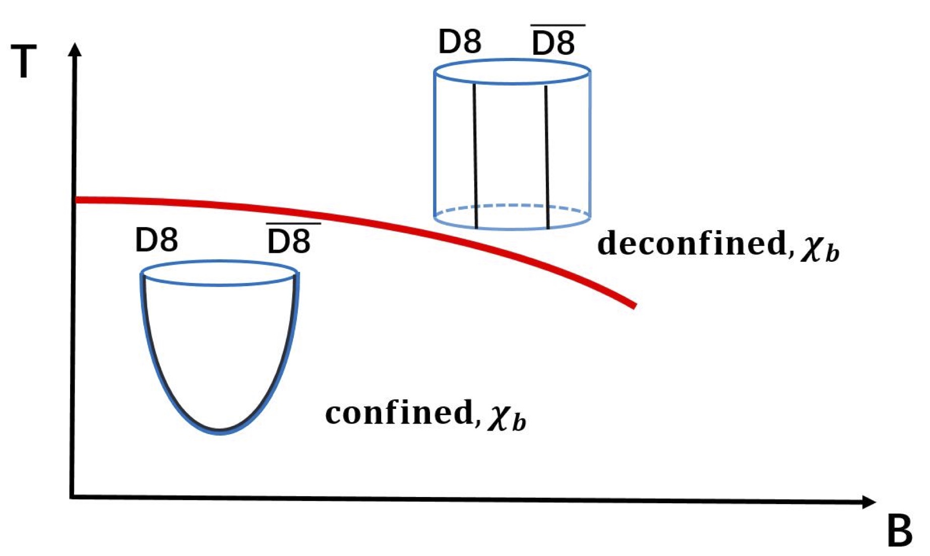
Figure 2: Holographic phase diagram V.S. lattice QCD result. Upper: The phase diagram in T-B plan from our holographic formula (6.12) (6.15). Lower: The phase diagram in T-B plan from some lattice QCD results in [1]. $N_{t}$ is a parameter in the lattice calculations.

6.2 The backreaction case

Let us turn to the case of backreaction. To get the phase diagram, first we need to imposing (4.1) and (4.2) on (5.9) and (5.13), thus obtain the pressure of each phase as,

$$p_{\mathrm{conf}.} =\frac{2N_{c}^{2}\lambda_{4}M_{KK}^{4}}{3^{7}\pi^{2}}\bigg{[}1-\frac{\lambda_{4}^{2}}{12\pi^{3}}\frac{N_{f}}{N_{c}}\bigg{(}-5A_{1}+A_{2}-\frac{2\pi^{3/2}\left(9+7\sqrt{3}\pi+21\log\frac{27}{16}\right)}{35\Gamma\left(-\frac{5}{3}\right)\Gamma\left(\frac{1}{6}\right)}$$

$$\ \ \ -\frac{1729\pi^{3/2}\left(72+\sqrt{3}\pi+3\log\frac{27}{16}\right)}{69984\Gamma\left(\frac{4}{3}\right)\Gamma\left(\frac{25}{6}\right)}q_{b}^{2}\bigg{)}\bigg{]},$$

$$p_{\mathrm{deconf}.} =\frac{128\pi^{4}N_{c}^{2}T^{6}\lambda_{4}}{2187M_{KK}^{2}}\left[1+\frac{\lambda_{4}^{2}}{12\pi^{3}}\frac{N_{f}}{N_{c}}\left(\frac{4}{7}-a_{1}-a_{2}+5a_{3}+\frac{14}{3}q_{b}^{2}\right)\right].$$ (6.14)

In order to obtain the critical temperature at the phase transition point, we could solve the equation $p_{\mathrm{deconf.}}(T=T_{c})=p_{\mathrm{conf.}}$ as in the probe approximation. Then we find the following relation between the critical temperature $T_{c}$ and the magnetic field $B$,

$$\frac{2\pi T_{c}}{M_{KK}} =1+\frac{N_{f}}{N_{c}}\left(X\lambda_{4}^{2}+\frac{B^{2}}{M_{KK}^{4}}Y\right),$$ (6.15)

where

$$X \simeq 0.0005,\ Y\simeq-2.44,$$ (6.16)

and we have also imposed the special choice (3.25) (3.46) to (6.15).

So similar to the case of the probe approximation, (6.15) shows the critical temperature increases by the effect of the flavors without magnetic field. Notice that the factor in front of the magnetic field is also negative which shows that the behavior of (6.15) is in agreement with the probe approximation. However, (6.15) should be a scheme-dependent statement thus it depends on the choices of the appropriate interpretation (also the numbers of colors and flavors). We have to keep this in mind, since we are less clear about the full relations between the integration constants and the constant magnetic field $B$, we therefore use the same ansatz as the most simple choice as [18] for the undetermined integration constants. The behavior of $T_{c}$ with $B$ (6.15) would be sensitive to the relations between the integration constants and the constant magnetic field.

Since the backreaction in our gravity solution is a perturbation, we could additionally require the following relations in order to omit the above ambiguities,

$$-5A_{1}+A_{2}-\frac{2\pi^{3/2}\left(9+7\sqrt{3}\pi+21\log\frac{27}{16}\right)}{35\Gamma\left(-\frac{5}{3}\right)\Gamma\left(\frac{1}{6}\right)}-\frac{1729\pi^{3/2}\left(72+\sqrt{3}\pi+3\log\frac{27}{16}\right)}{69984\left(\frac{4}{3}\right)\Gamma\left(\frac{25}{6}\right)}q_{b}^{2}$$

$$= \ \ \frac{32\pi^{3/2}}{21\Gamma\left(\frac{1}{6}\right)\Gamma\left(\frac{4}{3}\right)}+\frac{4\pi^{3/2}}{3\Gamma\left(\frac{1}{6}\right)\Gamma\left(\frac{4}{3}\right)}q_{b}^{2},$$ (6.17)

and

$$-a_{1}-a_{2}+5a_{3}+\frac{14}{3}q_{b}^{2}=2q_{b}^{2},$$ (6.18)

by comparing the thermodynamical quantities (6.14) with (6.6) (6.12) in the probe limit. It is consistent that our gravity solution does not describe the full reactions from the flavors, because all our calculations are in the Veneziano limit. On the other hand, it is not necessary to discuss the full D4-$\mathrm{D}8/\overline{\mathrm{D}8}$ solution since it provides a totally different holographic duality from the Witten-Sakai-Sugimoto model, which can not be described by our perturbative solution in Section 3. In this sense, according to (6.17) (6.18) with some special choices, all the integration constants could be determined by the thermodynamical constraints. However it implies that everything discussed in our manuscript can not go beyond the probe approximation in fact.

7 Summary and discussion

In this paper, by considering the backreaction of the flavors and the magnetic field, we have constructed gravitational solutions as a magnetic-dependently holographic background in the Witten-Sakai-Sugimoto model. Thus it corresponds to a large $N_{c}$ quantum field theory (or large $N_{c}$ QCD) with dynamical flavors in an external magnetic field. We have proved out our gravitational solutions satisfy their equations of motion explicitly in the first order of $N_{f}/N_{c}$. The solutions are analytic both in confined (bubble) and deconfined (black brane) case at low (zero) or high (finite) temperature. Therefore these solutions are able to study the the influence of dynamical flavors in an external magnetic field as a holographic version of [1, 2, 3, 4]. In order to determine the integration constants in our solutions, we require the backgrounds are completely regular in the IR region of the dual field theory as the unflavored case since the flavors are small perturbations. On the other hand, we also try to turn off the sources or VEVs of some gauge invariant operators in the dual field theory as another constraint. However the calculation shows it is not enough to determine all the integration constants just by these two constraints. So we have to keep those undetermined integration constants as some generic parameters temporarily.

In order to compare our magnetic-dependent case with [18], we simply chose the same value for the undetermined integration constants as [18], to study some physical properties about hadronic physics in an external magnetic field, such as the running coupling, (QCD) string tension, baryon mass. We find the UV behavior of the running coupling is not affected by the presence of the magnetic field. And the string tension, the mass of baryon increase by the presence of the flavor or the magnetic field. But we need to keep in mind these behaviors should depend on which scheme is chosen and where some observables is kept fixed in the theory since theories with different numbers of flavors might be different. Additionally, due to the simply choice as [18] for those undetermined integration constants, the results (in this part) are not strictly rigorous thus some of them might still seem unrealistic.

Moreover, it shows the physical significance of our work by investigating the holographic renormalization and thermodynamics with our magnetic-dependently gravitational solution. We employ the counterterm [29] and its covariant formula [18] for this model then evaluate them by our magnetic solution. The motivation for studying this counterterm is to renormalize the free energy, to study the Hawking-Page transition holographically in the presence of the magnetic field. In some applications of the Witten-Sakai-Sugimoto model, holographic renormalization may not be necessary for studying the phase transition. Since those concerns are the difference of the free energy of the various configurations of the flavor branes in the same background, which is not the Hawking-Page transition of this model. So the difference of the free energy could be finite in those approaches (such as [11, 15, 19, 16, 30]). However, in our calculations, holographic renormalization is needed since we (more than that) also consider the transition between differently geometric background. According to our calculations, if the parameters in the covariant counterterms are allowed to depend on the magnetic field as [29], we find the present counterterms are enough to cancel all the divergences.

In particular, after the holographic renormalization, we have concentrated the attention on the holographic phase diagrams in the presence of the magnetic field, and compare it with lattice QCD results. In our backreaction case, we find the pressure of both phases evaluated by our magnetic-dependent solution agrees with [29] qualitatively. Although the behavior of the phase diagram agrees with lattice QCD [1, 2], there might be a bit ambiguous since we have chosen the special value for the integration constants. In the probe approximation, the phase diagram is clear and also in agreement with the lattice QCD [1, 2] qualitatively (Figure 2). Thus it could be interpreted as the inhibition of confinement or chirally broken symmetry by the magnetic field holographically. Besides, we additionally require our backreaction solution coincides with the case of probe limit by the analyses of the thermodynamics, so that all the integration constants could be determined in this sense.

Finally, let us comment something more about our work. As an improvement to [29], we have employed the technique used in [18] to take into account the backreaction from flavors and the magnetic field. Because of the presence of the magnetic field, actually we need to solve a set of highly non-linear equations of motion first to obtain a magnetic-dependently gravitational solution, as shown in (3.17) and (3.37). Since it is hopeless to find an analytic solution from these extremely complicated equations, we solve them by keeping the leading $B^{2}$ terms. So while it is a challenge to keep all the orders of the DBI action to solve analytically, some numerical calculations might be worthy. Besides, during our calculations, we have restricted that $\mathrm{D}8/\overline{\mathrm{D}8}$-branes are placed at antipodal points of $x_{4}$ - circle in the confined phase. So to extend this part to the non-antipodal case would be natural, and the chiral symmetry could also be restored after deconfinement transition. Moreover, it is also interesting to turn on a chemical potential and a magnetic field together on the flavor branes in this framework, since a similar phenomena, named as “inverse magnetic catalysis”, has also been found by using this model in the probe approach of [19]. However, there would be a non-vanished Chern-Simons term necessarily if turning on the chemical potential and the magnetic field together as [19, 30]. It would be more difficult to search for an analytic solution even in the expansion of small baryon charge, magnetic field and $N_{f}/N_{c}$ in that case since the equations of motion would be complicatedly coupled to each other once the backreaction is considered. We would like to leave these interesting topics for a future study to improve our calculations about holographic QCD.

References

• [1] G. S. Bali, F. Bruckmann, G. Endrodi, Z. Fodor, S. D. Katz, S. Krieg, A. Schafer, K. K. Szabo, “The QCD phase diagram for external magnetic fields”, JHEP 1202 (2012) 044, [arXiv:1111.4956].
• [2] G. S. Bali, F. Bruckmann, G. Endrodi, S. D. Katz, A. Schafer, “The QCD equation of state in background magnetic fields”, JHEP 1408, 177 (2014), [arXiv:1406.0269].
• [3] Kenji Fukushima, Yoshimasa Hidaka, “Magnetic Catalysis vs Magnetic Inhibition”, PhysRevLett.110.031601, [arXiv:1209.1319].
• [4] Eduardo S. Fraga, Leticia F. Palhares, “Deconfinement in the presence of a strong magnetic background: an exercise within the MIT bag model”, Phys.Rev. D86 (2012) 016008.
• [5] Eduardo S. Fraga, Jorge Noronha, Leticia F. Palhares, “Large Nc Deconfinement Transition in the Presence of a Magnetic Field”, PhysRevD.87.114014, [arXiv:1207.7094].
• [6] J. M. Maldacena, “The large N limit of superconformal field theories and supergravity”, Adv. Theor. Math. Phys. 2, 231 (1998) [Int. J. Theor. Phys. 38, 1113 (1999)] [arXiv:hep-th/9711200].
• [7] E. Witten, “Anti-de Sitter space and holography”, Adv. Theor. Math. Phys. 2, 253 (1998), [arXiv:hep-th/9802150].
• [8] O. Aharony, S. S. Gubser, J. Maldacena, H. Ooguri and Y. Oz, “Large N Field Fheories, String Theory and Gravity”, Phys. Rept. 323 (2000) 183, [hep-th/9905111].
• [9] T. Sakai, S. Sugimoto, “Low energy hadron physics in holographic QCD,” Prog. Theor. Phys. 113, 843 (2005), [hep-th/0412141].
• [10] T. Sakai, S. Sugimoto, “More on a holographic dual of QCD”, Prog. Theor. Phys. 114, 1083 (2005) [arXiv:hep-th/0507073].
• [11] O. Aharony, J. Sonnenschein, S. Yankielowicz, “A Holographic model of deconfinement and chiral symmetry restoration”, Annals Phys. 322 (2007) 1420-1443, [hep-th/0604161].
• [12] Hiroyuki Hata, Tadakatsu Sakai, Shigeki Sugimoto, Shinichiro Yamato, “Baryons from instantons in holographic QCD”, Prog.Theor.Phys.117:1157 (2007), [arXiv:hep-th/0701280].
• [13] K. Hashimoto, T. Sakai and S. Sugimoto, “Nuclear Force from String Theory”, Prog. Theor. Phys. 122 (2009) 427, [arXiv:0901.4449 [hep-th]].
• [14] K. Hashimoto, N. Iizuka and Y. Piljin, “A Matrix Model for Baryons and Nuclear Forces”, JHEP 1010, 003(2010), [arXiv:1003.4988 [hep-th]].
• [15] Oren Bergman, Gilad Lifschytz, Matthew Lippert, “Holographic Nuclear Physics”, JHEP0711:056 (2007), [arXiv:0708.0326].
• [16] Si-wen Li, Andreas Schmitt, Qun Wang, “From holography towards real-world nuclear matter”, PhysRevD.92.026006, [arXiv:1505.04886].
• [17] Anton Rebhan, “The Witten-Sakai-Sugimoto model: A brief review and some recent results”, [arXiv:1410.8858].
• [18] Francesco Bigazzi, Aldo L. Cotrone, “Holographic QCD with Dynamical Flavors”, JHEP01(2015)104, [arXiv:1410.2443].
• [19] Florian Preis, Anton Rebhan, Andreas Schmitt, “Inverse magnetic catalysis in dense holographic matter”, JHEP 1103:033,2011, [arXiv:1012.4785].
• [20] Moshe Rozali, Hsien-Hang Shieh, Mark Van Raamsdonk, Jackson Wu, “Cold Nuclear Matter In Holographic QCD”, JHEP0801:053 (2008), [arXiv:0708.1322].
• [21] Kazuo Ghoroku, Kouki Kubo, Motoi Tachibana, Tomoki Taminato, Fumihiko Toyoda, “Holographic cold nuclear matter as dilute instanton gas ”, Phys.Rev. D87 (2013) no.6, 066006, [arXiv:1211.2499].
• [22] Gautam Mandal, Takeshi Morita, “Gregory-Laflamme as the confinement/deconfinement transition in holographic QCD”, JHEP 1109 (2011) 073, [arXiv:1107.4048].
• [23] Gautam Mandal, Takeshi Morita, “What is the gravity dual of the confinement/deconfinement transition in holographic QCD?”, J.Phys.Conf.Ser. 343 (2012) 012079, [arXiv:1111.5190].
• [24] F. Bigazzi, R. Casero, A. L. Cotrone, E. Kiritsis, A. Paredes, “Non-critical holography and four-dimensional CFT’s with fundamentals,” JHEP 0510, 012 (2005), [hepth/ 0505140].
• [25] R. Casero, C. Nunez, A. Paredes, “Towards the string dual of N=1 SQCD-like theories”, Phys. Rev. D 73, 086005 (2006), [hep-th/0602027].
• [26] F. Benini, F. Canoura, S. Cremonesi, C. Nunez and A. V. Ramallo, “Unquenched flavors in the Klebanov-Witten model,” JHEP 0702, 090 (2007), [hep-th/0612118].
• [27] C. Nunez, A. Paredes, A. V. Ramallo, “Unquenched Flavor in the Gauge/Gravity Correspondence,” Adv. High Energy Phys. 2010, 196714 (2010), [arXiv:1002.1088 [hepth]].
• [28] F. Bigazzi, A. L. Cotrone, J. Mas, D. Mayerson, J. Tarrio, “Holographic Duals of Quark Gluon Plasmas with Unquenched Flavors”, Commun. Theor. Phys. 57, 364 (2012) [arXiv:1110.1744 [hep-th]].
• [29] A. Ballon-Bayona, “Holographic deconfinement transition in the presence of a magnetic field,” JHEP 1311, 168 (2013), [arXiv:1307.6498 [hep-th]].
• [30] F. Preis, A. Rebhan, A. Schmitt, “Inverse magnetic catalysis in field theory and gauge-gravity duality”, Lect.Notes Phys. 871 (2013) 51-86, [arXiv:1208.0536].
• [31] Kiminad A. Mamo, “Inverse magnetic catalysis in holographic models of QCD”, JHEP05(2015)121, [arXiv:1501.03262].
• [32] E. Antonyan, J.A. Harvey, S. Jensen, D. Kutasov, “NJL and QCD from String Theory”, [arXiv:hep-th/0604017].
• [33] Joshua L. Davis, Michael Gutperle, Per Kraus, Ivo Sachs, “Stringy NJL and Gross-Neveu models at finite density and temperature”, JHEP0710:049(2007), [arXiv:0708.0589].
• [34] E. Witten, “Anti-de Sitter space, thermal phase transition, and connement in gauge theories,” Adv. Theor. Math. Phys. 2, 505 (1998) [hep-th/9803131].
• [35] Koji Hashimoto, Takashi Oka, Akihiko Sonoda, “Electromagnetic instability in holographic QCD”, JHEP 1506 (2015) 001, [arXiv:1412.4254].
• [36] Koji Hashimoto, Takashi Oka, Akihiko Sonoda, “Magnetic instability in AdS/CFT : Schwinger effect and Euler-Heisenberg Lagrangian of Supersymmetric QCD”, JHEP 1406 (2014) 085, [arXiv:1403.6336].
• [37] Koji Hashimoto, Takashi Oka, “Vacuum Instability in Electric Fields via AdS/CFT: Euler-Heisenberg Lagrangian and Planckian Thermalization”, JHEP 1310 (2013) 116, [arXiv:1307.7423].
• [38] I.R. Klebanov, A.A. Tseytlin, “D-Branes and Dual Gauge Theories in Type 0 String Theory”, Nucl.Phys.B546:155-181 (1999), [arXiv:hep-th/9811035].
• [39] F. Bigazzi, A. L. Cotrone, L. Martucci, L. A. Pando Zayas, “Wilson loop, Regge trajectory and hadron masses in a Yang-Mills theory from semiclassical strings,” Phys. Rev. D 71, 066002 (2005) [hep-th/0409205].
• [40] Alejandro Ayala, C. A. Dominguez, L. A. Hernandez, M. Loewe, R. Zamora, “The magnetized effective QCD phase diagram”, Phys. Rev. D 92, 096011 (2015), [arXiv:1509.03345].
• [41] D. Giataganas, N. Irges, “Flavor Corrections in the Static Potential in Holographic QCD,” Phys. Rev. D 85, 046001 (2012), [arXiv:1104.1623 [hep-th]].
• [42] E. Witten, “Baryons and branes in anti-de Sitter space,” JHEP 9807, 006 (1998), [hep-th/ 9805112].
• [43] David J. Gross, Hirosi Ooguri, “Aspects of Large N Gauge Theory Dynamics as Seen by String Theory”, Phys. Rev. D 58, 106002, [arXiv:hep-th/9805129].
• [44] D. Mateos, R. C. Myers, R. M. Thomson, “Thermodynamics of the brane,” JHEP 0705, 067 (2007), [hep-th/0701132].
• [45] D. Dudal, D. R. Granado, T. G. Mertens, “On (no) inverse magnetic catalysis in the QCD hard and soft wall models”, [arXiv:1511.04042].
• [46] Hui Li, Xin-li Sheng, Qun Wang, “Electromagnetic fields with electric and chiral magnetic conductivities in heavy ion collisions”, [arXiv:1602.02223].