APPROXIMATIONS FOR THE CAPUTO DERIVATIVE (II)

Abstract

In the present paper we use the expansion formula of the polylogarithm function to construct approximations of the Caputo derivative which are related to the midpoint approximation of the integral in the definition of the Caputo derivative. The asymptotic expansion formula of the Riemann sum approximation of the beta function and the first terms of the expansion formulas of the approximations of the Caputo derivative of the power function are obtained in the paper. The induced shifted approximations of the Grünwald formula and the approximations of the Caputo derivative studied in the first part of the paper are constructed and applied for numerical solution of fractional differential equations.
MSC 2010: 65D30, 26A33, 34A08, 42A38, 65D32.
Key Words and Phrases: fractional derivative, approximation, Fourier transform, asymptotic expansion formula, fractional differential equation.

1 Introduction

The finite difference schemes for numerical solution of ordinary and partial fractional differential equations (FDEs) involve approximations of the fractional derivatives. The fractional integral of order $\alpha>0$ and the Caputo fractional derivative of order $\alpha$, where $0<\alpha<1$ are defined as

$$I^{\alpha}y(t)=\dfrac{1}{\Gamma(\alpha)}\int_{0}^{t}(t-x)^{\alpha-1}y(x)dx,$$

$$y^{(\alpha)}(t)=D^{\alpha}y(t)=\dfrac{1}{\Gamma(1-\alpha)}\int_{0}^{t}\dfrac{y^{\prime}(x)}{(t-x)^{\alpha}}dx.$$ (1.1)

The Caputo derivative of the exponential function is expressed with the Mittag-Leffler function as $D^{\alpha}e^{t}=t^{1-\alpha}E_{1,2-\alpha}(t)$. The Caputo derivatives of the sine and cosine functions satisfy

$$D^{\alpha}\sin t=t^{1-\alpha}E_{2,2-\alpha}\left(-t^{2}\right),\;D^{\alpha}\cos t=-t^{2-\alpha}E_{2,3-\alpha}\left(-t^{2}\right).$$

Let $h=t/n$, where $n$ is a positive integer, and $t_{m}=mh$, $y_{m}=y(t_{m})$. The L1 approximation for the Caputo derivative is a commonly used approximation for numerical solution of fractional differential equations [7, 18, 24].

$$\dfrac{1}{\Gamma(2-\alpha)h^{\alpha}}\sum_{k=0}^{n}\sigma_{k}^{(\alpha)}y_{n-k}=y^{(\alpha)}_{n}+O\left(h^{2-\alpha}\right),$$ (1.2)

where $\sigma_{0}^{(\alpha)}=1$, $\sigma_{n}^{(\alpha)}=(n-1)^{1-\alpha}-n^{1-\alpha}$ and

$$\sigma_{k}^{(\alpha)}=(k+1)^{1-\alpha}-2k^{1-\alpha}+(k-1)^{1-\alpha},\quad(k=2,\cdots,n-1).$$

The weights $\sigma_{k}^{(\alpha)}$ of the L1 approximation have the following properties

$$(i)\quad\sigma_{0}^{(\alpha)}>0,\;\sigma_{1}^{(\alpha)}<\sigma_{2}^{(\alpha)}<\cdots<\sigma_{k}^{(\alpha)}<\cdots<\sigma_{n-1}^{(\alpha)}<0,\;\sigma_{n}^{(\alpha)}<0,$$

$$(ii)\quad\sum_{k=0}^{n}\sigma_{k}^{(\alpha)}=0,\quad\sum_{k=1}^{n}k\sigma_{k}^{(\alpha)}=-n^{1-\alpha},$$ (1.3)

$$(iii)\quad\sigma_{k}^{(\alpha)}=\dfrac{C_{1}}{k^{1+\alpha}}+O\left(\dfrac{1}{k^{2+\alpha}}\right),\quad\sigma_{n}^{(\alpha)}=\dfrac{C_{2}}{n^{\alpha}}+O\left(\dfrac{1}{n^{1+\alpha}}\right),$$

where $C_{1}=\alpha(\alpha-1)$ and $C_{2}=\alpha-1$. When the function $y\in C^{2}[0,t_{n}]$, the L1 approximation of the Caputo derivative has an order $2-\alpha$ ([22]). The L1 approximation is constructed by using a linear interpolation of the integrand function on all subintervals $[t_{m-1},t_{m}]$. Approximations of fractional integrals and derivatives is an active research field. Higher order approximations of the fractional derivative which use a Lagrange polynomial or spline interpolation of the integrand function are studied by Odibat [25], Li, Chen and Ye [20], Sousa [30], Chen and Deng [3], Gao, Sun and Zhang [15], Yan, Pal and Ford [37], Alikhanov [2], Li, Cao and Li [21], Kumar, Pandey and Sharma [19]. Algorithms for computation of the Caputo derivative in $O(N\ln^{2}N)$ time are studied by Jiang et al. [17], Yan, Sun and Zhang [38], Ren, Mao and Zhang [27]. The two-term equation is a basic ordinary FDE. When $0<\alpha<1$ the two-term FDE is called fractional relaxation equation.

$$y^{(\alpha)}(t)+y(t)=F(t),\quad y(0)=y_{0}.$$ (1.4)

Suppose that

$$\dfrac{1}{h^{\alpha}}\sum_{k=0}^{n}\lambda_{k}^{(\alpha)}y_{n-k}=y_{n}^{(\alpha)}+O\left(h^{\beta(\alpha)}\right)$$ (*)

is an approximation of the Caputo derivative. The numerical solution of the two term equation (1.4) of order $\beta(\alpha)$, which uses approximation (*) of the Caputo derivative is computed with $u_{0}=y_{0}$ and [7, 9, 11]

$$u_{n}=\dfrac{1}{\lambda_{0}^{(\alpha)}+h^{\alpha}}\left(h^{\alpha}F_{n}-\sum_{k=1}^{n}\lambda_{k}^{(\alpha)}u_{n-k}\right).$$ (NS1(*))

In the first part of the paper [9] we study the numerical solutions of the two-term equations

$$y^{(\alpha)}(t)+y(t)=1 +t+t^{2}+t^{3}+t^{4}+\dfrac{t^{1-\alpha}}{\Gamma(2-\alpha)}$$ (1.5)

$$+\dfrac{2t^{2-\alpha}}{\Gamma(3-\alpha)}+\dfrac{6t^{3-\alpha}}{\Gamma(4-\alpha)}+\dfrac{24t^{4-\alpha}}{\Gamma(5-\alpha)},\quad y(0)=1,$$

$$y^{(\alpha)}(t)+y(t)=e^{t}+t^{1-\alpha}E_{1,2-\alpha}(t),\quad y(0)=1,$$ (1.6)

$$y^{(\alpha)}(t)+y(t)=\cos(2\pi t)-4\pi^{2}t^{1-\alpha}E_{2,3-\alpha}(-4\pi^{2}t^{2}),\quad y(0)=1.$$ (1.7)

Two-term equations (1.5), (1.6), (1.7) have the solutions $y(t)=1+t+t^{2}+t^{3}+t^{4},\;y(t)=e^{t},\;y(t)=\cos(2\pi t).$ The numerical results for the error and the order of numerical solution NS1(1.2), which uses the L1 approximation of the Caputo derivative of two-term equation (1.5) and $\alpha=0.25$, equation (1.6),$\alpha=0.5$ and equation (1.7), $\alpha=0.75$ are presented in Table 1. The errors of the numerical solutions are computed on the interval $[0,1]$ with respect to the maximum $l_{\infty}$ norm. The Riemann zeta function is a special function defined as

$$\zeta(\alpha)=\displaystyle{\sum_{n=1}^{\infty}\dfrac{1}{n^{\alpha}}},\;(\alpha>1),\quad\zeta(\alpha)=\displaystyle{\dfrac{1}{1-2^{1-\alpha}}\sum_{n=1}^{\infty}\dfrac{(-1)^{n-1}}{n^{\alpha}}},\;(\alpha>0).$$

The Euler-Mclaurin formula

$$h\left(\dfrac{y(0)}{2}+\sum_{k=1}^{n-1}y(kh)+\dfrac{y(t)}{2}\right)= \int_{0}^{t}y(\xi)d\xi+$$ (1.8)

$$\sum_{n=1}^{\infty}2(-1)^{n+1}\zeta(2n) \left(y^{(2n-1)}(t)-y^{(2n-1)}(0)\right)\left(\dfrac{h}{2\pi}\right)^{2n}$$

and the expansion formulas of the approximations of the fractional integrals and derivatives involve the values of the zeta function. In [7, 8] we use the formula for sum of powers

$$\sum_{k=1}^{n-1}k^{\alpha}=\zeta(-\alpha)+\dfrac{n^{1+\alpha}}{1+\alpha}\sum_{m=0}^{\infty}\binom{\alpha+1}{m}\dfrac{B_{m}}{n^{m}}.$$

to derive the expansion formula of the L1 approximation

$$\dfrac{1}{\Gamma(2-\alpha)h^{\alpha}}\sum_{k=0}^{n}\sigma_{k}^{(\alpha)}y(t-kh)=y^{(\alpha)}(t)+ \dfrac{\zeta(\alpha-1)}{\Gamma(2-\alpha)}y^{\prime\prime}(t)h^{2-\alpha}+O\left(h^{2}\right),$$

and a second-order approximation for the Caputo derivative by modifying the first three weights of the L1 approximation with the value of the zeta function $\zeta(\alpha-1)$.

$$y^{(\alpha)}_{n}=\dfrac{1}{\Gamma(2-\alpha)h^{\alpha}}\sum_{k=0}^{n}\delta_{k}^{(\alpha)}y_{n-k}+O\left(h^{2}\right),$$ (1.9)

where $\delta_{k}^{(\alpha)}=\sigma_{k}^{(\alpha)}$ for $2\leq k\leq n$ and

$$\delta_{0}^{(\alpha)}=\sigma_{0}^{(\alpha)}-\zeta(\alpha-1),\;\delta_{1}^{(\alpha)}=\sigma_{1}^{(\alpha)}+2\zeta(\alpha-1),\;\delta_{2}^{(\alpha)}=\sigma_{2}^{(\alpha)}-\zeta(\alpha-1).$$

The Riemann zeta function is a special case $(t=1)$ of the polylogarithm function defined as

$$Li_{\alpha}(t)=\sum_{n=1}^{\infty}\dfrac{t^{n}}{n^{\alpha}}=t+\dfrac{t^{2}}{2^{\alpha}}+\cdots+\dfrac{t^{n}}{n^{\alpha}}+\cdots\qquad(|t|<1).$$

The polylogarithm function has properties

$$Li_{\alpha}(t)+Li_{\alpha}(-t)=2^{1-\alpha}Li_{\alpha}(t^{2}),$$ (1.10)

$$Li_{\alpha}(t)=\Gamma(1-\alpha)\left(\ln\dfrac{1}{t}\right)^{\alpha-1}+\sum_{n=0}^{\infty}\dfrac{\zeta(\alpha-n)}{n!}\left(\ln t\right)^{n},$$ (1.11)

where $\alpha\neq 1,2,3,\cdots$ and $|\ln t|<2\pi$. From (1.11) with $t=e^{i\omega h}$ we obtain

$$Li_{\alpha}\left(e^{iwh}\right)=\Gamma(1- \alpha)(-iw)^{\alpha-1}h^{\alpha-1}+\zeta(\alpha)-(-iw)\zeta(\alpha-1)h$$ (1.12)

$$+(-iw)^{2}\dfrac{\zeta(\alpha-2)}{2}h^{2}-(-iw)^{3}\dfrac{\zeta(\alpha-3)}{6}h^{3}+O\left(h^{4}\right).$$

In [9] we use (1.12) to obtain approximations of the Caputo derivative and their expansion formulas:

$$\dfrac{1}{2\Gamma(1-\alpha)h^{\alpha}}\sum_{k=0}^{n}\sigma_{k}^{(\alpha)}y_{n-k}=y_{n}^{(\alpha)}+O\left(h^{2-\alpha}\right),$$ (1.13)

where $\sigma_{0}^{(\alpha)}=1-2\zeta(\alpha),\;\sigma_{1}^{(\alpha)}=\dfrac{1}{2^{\alpha}}+2\zeta(\alpha)$ and

$$\sigma_{k}^{(\alpha)}=\dfrac{1}{(k+1)^{\alpha}}-\dfrac{1}{(k-1)^{\alpha}},\quad(k=2,\cdots,n).$$

Approximation (1.13) has an order $2-\alpha$ when the function $y(t)\in C^{2}[0,t_{n}]$ and satisfies the condition $y(0)=y^{\prime}(0)=0$. The approximation is extended to all functions of the class $C^{2}[0,t_{n}]$ by applying a modification of the last two weights $\sigma_{n-1}^{(\alpha)}$ and $\sigma_{n}^{(\alpha)}$:

$$\sigma_{n-1}^{(\alpha)}=-\dfrac{1}{(n-2)^{\alpha}}-2\left(\sum_{k=1}^{n-1}\frac{1}{k^{\alpha}}-\frac{n^{1-\alpha}}{1-\alpha}-\zeta(\alpha)\right),$$

$$\sigma_{n}^{(\alpha)}=-\dfrac{1}{(n-1)^{\alpha}}+2\left(\sum_{k=1}^{n-1}\frac{1}{k^{\alpha}}-\frac{n^{1-\alpha}}{1-\alpha}-\zeta(\alpha)\right).$$

$$\dfrac{1}{\Gamma(-\alpha)h^{\alpha}}\sum_{k=0}^{n}\sigma_{k}^{(\alpha)}y_{n-k}=y_{n}^{(\alpha)}+O\left(h^{2-\alpha}\right),$$ (1.14)

where $\sigma_{0}^{(\alpha)}=\zeta(\alpha)-\zeta(1+\alpha),\;\sigma_{1}^{(\alpha)}=1-\zeta(\alpha)$ and

$$\sigma_{k}^{(\alpha)}=\dfrac{1}{k^{1+\alpha}},\quad(k=2,\cdots,n),$$

and modified weights $\sigma_{n-1}^{(\alpha)}$ and $\sigma_{n}^{(\alpha)}$:

$$\sigma_{n-1}^{(\alpha)}=\dfrac{1}{(n-1)^{1+\alpha}}-\dfrac{n^{1-\alpha}}{\alpha(1-\alpha)}+n\left(\zeta(1+\alpha)-\sum_{k=1}^{n-1}\dfrac{1}{k^{1+\alpha}}\right)-\left(\zeta(\alpha)-\sum_{k=1}^{n-1}\dfrac{1}{k^{\alpha}}\right),$$

$$\sigma_{n}^{(\alpha)}=(1-n)\left(\zeta(1+\alpha)-\sum_{k=1}^{n-1}\dfrac{1}{k^{1+\alpha}}\right)+\left(\zeta(\alpha)-\sum_{k=1}^{n-1}\dfrac{1}{k^{\alpha}}\right)+\dfrac{n^{1-\alpha}}{\alpha(1-\alpha)}.$$

The exponential Fourier transform of the function $y$ is defined as

$$\mathcal{F}[y(t)](w)=\hat{y}(w)=\int_{-\infty}^{\infty}e^{iwt}y(t)dt.$$

The Fourier transform has properties $\mathcal{F}[y(t-b)](w)=e^{iwb}\hat{y}(w)$ and

$$\mathcal{F}[D^{\alpha}y(t)](w)=(-iw)^{\alpha}\hat{y}(w),\quad\mathcal{F}[I^{\alpha}y(t)](w)=(-iw)^{-\alpha}\hat{y}(w).$$

The generating function and the expansion formulas of an approximation are related to the Fourier transform of the approximation. Approximations for the Caputo derivative, constructed from the properties of the Fourier transform and the generating function of the approximation, are studied by Tadjeran, Meerschaert and Scheffer [31], Tian, Zhou and Deng [32], Ding and Li [12, 13], Dimitrov [9], Ren and Wang [28]. In section 3 we use Fourier transform and (1.12) to construct approximations of the Caputo derivative and their expansion formulas which are related to the midpoint approximation of the fractional integral (1) in the definition of the Caputo derivtive.

$$\dfrac{1}{\Gamma(1-\alpha)h^{\alpha}}\sum_{k=0}^{n}\sigma_{k}^{(\alpha)}y_{n-k}=y_{n}^{(\alpha)}+O\left(h^{2-\alpha}\right),$$ (1.15)

where

$$\sigma_{0}^{(\alpha)}=2^{\alpha}-\left(2^{\alpha}-1\right)\zeta(\alpha),\quad\sigma_{1}^{(\alpha)}=\left(\dfrac{2}{3}\right)^{\alpha}-2^{\alpha}+\left(2^{\alpha}-1\right)\zeta(\alpha),$$

$$\sigma_{k}^{(\alpha)}=2^{\alpha}\left(\dfrac{1}{(2k+1)^{\alpha}}-\dfrac{1}{(2k-1)^{\alpha}}\right),\quad(k=2,\cdots,n),$$

and modified weights $\sigma_{n-1}^{(\alpha)}$ and $\sigma_{n}^{(\alpha)}$:

$$\sigma_{n-1}^{(\alpha)}=\dfrac{2^{\alpha}}{(2n-1)^{\alpha}}-\dfrac{2^{\alpha}}{(2n-3)^{\alpha}}+\frac{n^{1-\alpha}}{1-\alpha}-\zeta(\alpha)-2^{\alpha}\left(\sum_{k=1}^{n}\dfrac{1}{(2k-1)^{\alpha}}-\zeta(\alpha)\right),$$

$$\sigma_{n}^{(\alpha)}=-\dfrac{2^{\alpha}}{(2n-1)^{\alpha}}+\zeta(\alpha)-\frac{n^{1-\alpha}}{1-\alpha}+2^{\alpha}\left(\sum_{k=1}^{n}\dfrac{1}{(2k-1)^{\alpha}}-\zeta(\alpha)\right).$$

$$\dfrac{1}{\Gamma(1-\alpha)h^{\alpha}}\sum_{k=0}^{n}\delta_{k}^{(\alpha)}y_{n-k}=y_{n}^{(\alpha)}+O\left(h^{2}\right),$$ (1.16)

where $\delta_{0}^{(\alpha)}=2^{\alpha}+\dfrac{3}{2}\left(1-2^{\alpha}\right)\zeta(\alpha)+\left(2^{\alpha-1}-1\right)\zeta(\alpha-1),$

$$\delta_{1}^{(\alpha)}=2^{\alpha}\left(\dfrac{1}{3^{\alpha}}-1\right)-2\left(1-2^{\alpha}\right)\zeta(\alpha)-2\left(2^{\alpha-1}-1\right)\zeta(\alpha-1),$$

$$\delta_{2}^{(\alpha)}=2^{\alpha}\left(\dfrac{1}{5^{\alpha}}-\dfrac{1}{3^{\alpha}}\right)+\dfrac{1}{2}\left(1-2^{\alpha}\right)\zeta(\alpha)+\left(2^{\alpha-1}-1\right)\zeta(\alpha-1),$$

$$\delta_{k}^{(\alpha)}=\sigma_{k}^{(\alpha)},\qquad(3\leq k\leq n),$$

where $\sigma_{k}^{(\alpha)}$ are the weights of approximation (1.15). The L1 approximation (1.2) and approximations (1.13), (1.14), (1.15) have an order $2-\alpha$ and their weights satisfy (1). The properties of the weights are used in the proofs for the convergence of the numerical solutions as well as to determine and improve the accuracy of the approximations when $n$ is small. The accuracy of the numerical solutions of order $2-\alpha$ which use approximations (1.2),(1.13),(1.14) and (1.15) for the Caputo derivative depends on the truncations error of the approximations and the absolute value of the coefficient $C(\alpha)$ of the term $C(\alpha)y^{\prime\prime}(t)h^{2-\alpha}$ in the asymptotic expansion formulas. Approximations (1.2),(1.13),(1.14) and (1.15) have coefficients

$$C_{2}(\alpha)=\frac{\zeta(\alpha-1)}{\Gamma(2-\alpha)},C_{13}(\alpha)=\frac{\zeta(\alpha)-2\zeta(\alpha-1)}{2\Gamma(1-\alpha)},C_{14}(\alpha)=\frac{\zeta(\alpha)-\zeta(\alpha-1)}{2\Gamma(-\alpha)},$$

$$C_{15}(\alpha)=\frac{\left(2-2^{\alpha}\right)\zeta(\alpha-1)-\left(2^{\alpha}-1\right)\zeta(\alpha)}{2\Gamma(1-\alpha)}.$$

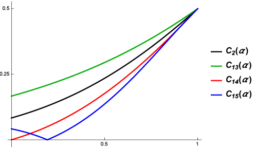
Figure 1: Graph of the absolute values of coefficients $C_{2}(\alpha)$, $C_{13}(\alpha)$, $C_{14}(\alpha)$ and $C_{15}(\alpha)$ for $0<\alpha<1$.

The absolute values of the coefficients $C_{14}(\alpha)$ and $C_{15}(\alpha)$ are smaller than the absolute value $|C_{1}(\alpha)|$ of the coefficient of the L1 approximation and $|C_{13}(\alpha)|>|C_{1}(\alpha)|$ (Figure 1). In the first part of this paper [9] we show that the errors of numerical solution NS1(1.14) of two-term equations (1.5), (1.6) and (1.7) are smaller than the errors of numerical solution NS1(1.2), while the corresponding errors of numerical solution NS1(1.13) are larger. The same pattern is observed when we compare the accuracy of numerical solution NS1(1.15) to the accuracy of numerical solutions NS1(1.2) and NS1(1.13) for standard FDEs. The errors of numerical solution NS(1.15) of equations (1.5), (1.6) and (1.7) are smaller than the errors of numerical solution NS1(1.2), which uses the L1 approximation of the Caputo derivative (Table 1 and Table 3). In section 4 we construct a finite difference scheme for numerical solution of the fractional subdiffusion equation, which uses approximation (1.15) of the Caputo derivative and we analyze the convergence of the scheme. In section 5 we derive the expansion formula of the Riemann sum approximation of the beta function and the asymptotic expansion formula

$$\sum_{k=1}^{n-1}k^{\beta}(n-k)^{\alpha}=\dfrac{\Gamma(\alpha+1)\Gamma(\beta+1)}{\Gamma(\alpha+\beta+2)} n^{\alpha+\beta+1}+\sum_{k=0}^{\infty}(-1)^{k}\binom{\beta}{k}\zeta(-\alpha-k)n^{\beta-k}$$

$$+\sum_{k=0}^{\infty} (-1)^{k}\binom{\alpha}{k}\zeta(-\beta-k)n^{\alpha-k}.$$ (1.17)

The Grüwald formula approximation of the Caputo derivative has a right endpoint expansion:

$$\dfrac{1}{h^{\alpha}}\sum_{k=0}^{N-1}(-1)^{k}\binom{\alpha}{k}y(t-kh)=y^{(\alpha)}(t)+\sum_{k=1}^{M-1}\dfrac{B_{k}^{(-\alpha)}(-\alpha)}{k!}y^{(k+\alpha)}(t)h^{k}+O\left(h^{M}\right),$$

where $B^{(\beta)}(t)$ are the generalized Bernoulli polynomials. When $y(0)=0$ the Grünwald formula approximates the Caputo derivative with a first order accuracy. The Grünwald formula is a second order approximation of the Caputo derivative with a shift parameter $s=S_{0}(\alpha)=\alpha/2$, when the function $y(t)$ satisfies $y(0)=y^{\prime}(0)=0$. Tian, Zhou and Deng [32] construct a class of second order shifted Grünwald difference (WSGD) approximations. The consruction of the WSGD operators uses a weighted average of shifted Grünwald formula approximations. Alekhanov [2] constructs a shifted approximation of the Caputo derivative of order $2-\alpha$. The approximation is called $\text{L2-1}_{s}$ formula and has an optimal shift value $s=\alpha/2$ (in the notations of this paper), where the approximation has an order $3-\alpha$. In [10] we construct shifted approximations of order $2-\alpha$ and two which have a shift parameter $s=\alpha/2$. In section 5 and section 6 we use (1) to show that the first term of the left endpoint expansions of approximations (1.2), (1.13), (1.14), (1.15) and the shifted Grünwald formula approximation of the power function $t^{\beta}$ is $Ch^{1+\beta}$, where $C=\zeta(-\beta)t^{-1-\alpha}/\Gamma(-\alpha)$. In section 6 we extend the method from [10] and we construct the induced shifted approximations of the Caputo derivative of approximations (1.2), (1.13), (1.14), (1.15) and the Grünwald formula approximation. The induced shifted approximations of (1.2), (1.13), (1.14), (1.15) have an order $2-\alpha$ and a second order accuracy at the optimal shift values. The induced shifted Grünwald formula approximation has a second order accuracy for an arbitrary shift value and a third order accuracy at the optimal shift value. In the special case when the shift value is equal to zero the induced Grünwald formula approximation is a second order approximation of the Caputo derivative for all functions $y\in C^{2}[0,t_{n}]$.

$$\dfrac{1}{h^{\alpha}}\sum_{k=0}^{N}\gamma_{k}^{(\alpha)}y_{n-k}=y_{n}^{(\alpha)}+O(h^{2}),$$ (1.18)

where

$$\gamma_{k}^{(\alpha)}=(-1)^{k}\binom{\alpha}{k}\frac{\alpha^{2}+3\alpha-2k+2}{2(\alpha-k+1)},\quad(k=0,\cdots,n-2),$$

$$\gamma_{n-1}^{(\alpha)}=(-1)^{n-1}\binom{\alpha-1}{n-2}\frac{2\alpha^{3}-\alpha^{2}n+4\alpha^{2}-5\alpha n+6\alpha+2n^{2}-4n}{2(\alpha-1)(\alpha-n+2)}+\dfrac{n^{1-\alpha}}{\Gamma(2-\alpha)},$$

$$\gamma_{n}^{(\alpha)}=(-1)^{n}\binom{\alpha-1}{n-2}\frac{\alpha^{2}+\alpha-2n+2}{2(\alpha-1)}-\dfrac{n^{1-\alpha}}{\Gamma(2-\alpha)}.$$

2 Approximation for the Caputo derivative of order 4-

Approximation (1.13) is constructed in [9] and it is related to the trapezoidal approximation for the fractional integral in the definition of the Caputo derivative (1). The absolute value of the coefficient $C_{13}(\alpha)$ of the term of order ${2-\alpha}$ in the expansion formula of approximation (1.13) is greater than the absolute value of the coefficient $C_{2}(\alpha)$ of the L1 approximation. In this section we use the Fourier transform and (1.12) to derive approximations (1.15) and (1.16) for the Caputo derivative, and their expansion formulas of order $4-\alpha$, which are related to the the midpoint approximation of the fractional integral in the definition of the Caputo derivative. The absolute value of the coefficient $C_{15}(\alpha)$ of the term of order $2-\alpha$ in the expansion formula of approximation (1.15) is smaller than $|C_{2}(\alpha)|$. From the midpoint approximation for the fractional integral in the definition of the Caputo derivative:

$$y^{(\alpha)}(t)\approx\dfrac{h}{\Gamma(1-\alpha)}\sum_{k=1}^{n}\dfrac{y^{\prime}\left(t_{k-1/2}\right)}{(t-t_{k-1/2})^{\alpha}}=\dfrac{h^{1-\alpha}}{\Gamma(1-\alpha)}\sum_{k=1}^{n}\dfrac{y^{\prime}_{k-1/2}}{(n-k+1/2)^{\alpha}}.$$

By approximating $y^{\prime}_{k-1/2}\approx(y_{k}-y_{k-1})/{h}$ we obtain

$$y^{(\alpha)}(t)\approx\dfrac{2^{\alpha}h^{1-\alpha}}{\Gamma(1-\alpha)}\sum_{k=1}^{n}\dfrac{y^{\prime}_{k-1/2}}{(2n-2k+1)^{\alpha}}\approx\dfrac{2^{\alpha}}{\Gamma(1-\alpha)h^{\alpha}}\sum_{k=1}^{n}\dfrac{y_{k}-y_{k-1}}{(2n-2k+1)^{\alpha}}.$$

Substitute $K=n-k$

$$\Gamma(1-\alpha)\left(\dfrac{h}{2}\right)^{\alpha}y^{(\alpha)}(t)\approx\sum_{K=0}^{n-1}\dfrac{y_{n-K}-y_{n-K+1}}{(2K+1)^{\alpha}}=\sum_{k=0}^{n-1}\dfrac{y_{n-K}}{(2K+1)^{\alpha}}-\sum_{k=0}^{n-1}\dfrac{y_{n-K+1}}{(2K+1)^{\alpha}},$$

$$y^{(\alpha)}(t)\approx\dfrac{2^{\alpha}}{\Gamma(1-\alpha)h^{\alpha}}\left(\sum_{k=0}^{n-1}\dfrac{y_{n-k}}{(2k+1)^{\alpha}}-\sum_{k=1}^{n}\dfrac{y_{n-k}}{(2k-1)^{\alpha}}\right).$$ (2.19)

Now we use Fourier transform and (1.12) to obtain the asymptotic expansion formula of approximation (2.19) of order $4-\alpha$. Denote

$$S^{(\alpha)}_{n}[y(t)]=\sum_{k=0}^{n-1}\dfrac{y_{n-k}}{(2k+1)^{\alpha}}-\sum_{k=1}^{n}\dfrac{y_{n-k}}{(2k-1)^{\alpha}}.$$ (2.20)

$$S^{(\alpha)}_{n}[y(t)]=y_{n}+\sum_{k=1}^{n-1}\left(\dfrac{1}{(2k+1)^{\alpha}}-\dfrac{1}{(2k-1)^{\alpha}}\right)y_{n-k}-\dfrac{y_{0}}{(2n-1)^{\alpha}}.$$ (2.21)

By applying Fourier transform to (2.20):

$$\mathcal{F}[S^{(\alpha)}_{\infty}[y(t)]](w)=\left(\sum_{k=0}^{\infty}\dfrac{e^{iwkh}}{(2k+1)^{\alpha}}-\sum_{k=1}^{\infty}\dfrac{e^{iwkh}}{(2k-1)^{\alpha}}\right)\hat{y}(w).$$

Denote $W=e^{iwh/2}$.

$$\mathcal{F}[S^{(\alpha)}_{\infty}[y(t)]](w) =\left(\sum_{k=0}^{\infty}\dfrac{W^{2k}}{(2k+1)^{\alpha}}-\sum_{k=1}^{\infty}\dfrac{W^{2k}}{(2k-1)^{\alpha}}\right)\hat{y}(w),$$

$$=\hat{y}(w)\left(\dfrac{1}{W}-W\right)\sum_{k=1}^{\infty}\dfrac{W^{2k-1}}{(2k-1)^{\alpha}}.$$

From (1.10)

$$2\sum_{k=1}^{\infty}\dfrac{W^{2k-1}}{(2k-1)^{\alpha}} =Li_{\alpha}(W)-Li_{\alpha}(-W)=2Li_{\alpha}(W)-Li_{\alpha}(W)-Li_{\alpha}(-W)$$

$$=2Li_{\alpha}(W)-2^{1-\alpha}Li_{\alpha}\left(W^{2}\right).$$

Hence

$$\mathcal{F}[S^{(\alpha)}_{\infty}[y(t)]](w)=\hat{y}(w)\left(e^{-\frac{iwh}{2}}-e^{\frac{iwh}{2}}\right)\left(Li_{\alpha}(e^{\frac{iwh}{2}})-\dfrac{1}{2^{\alpha}}Li_{\alpha}\left(e^{iwh}\right)\right).$$

The exponential function satisfies

$$e^{-\frac{iwh}{2}}-e^{\frac{iwh}{2}}=(-iwh)+\dfrac{(-iwh)^{3}}{24}+O\left(h^{5}\right).$$ (2.22)

From (1.12) the function $Li_{\alpha}\left(e^{\frac{iwh}{2}}\right)$ has a fourth-order series expansion

$$Li_{\alpha}\left(e^{\frac{iwh}{2}}\right)=\dfrac{\Gamma(1-\alpha)}{2^{\alpha-1}} (-iwh)^{\alpha-1}+\zeta(\alpha)-(-iw)\dfrac{\zeta(\alpha-1)}{2}h$$ (2.23)

$$+(-iw)^{2} \dfrac{\zeta(\alpha-2)}{8}h^{2}-(-iw)^{3}\dfrac{\zeta(\alpha-3)}{48}h^{3}+O\left(h^{4}\right).$$

From (1.12) and (2.23) we obtain

$$Li_{\alpha}\left(e^{\frac{iwh}{2}}\right) -\dfrac{1}{2^{\alpha}}Li_{\alpha}\left(e^{iwh}\right)=\dfrac{\Gamma(1-\alpha)}{2^{\alpha}}(-iw)^{\alpha-1}h^{\alpha-1}+\left(1-\dfrac{1}{2^{\alpha}}\right)\zeta(\alpha)$$

$$-(-i w)\left(\dfrac{1}{2}-\dfrac{1}{2^{\alpha}}\right)\zeta(\alpha-1)h+(-iw)^{2}\dfrac{1}{2}\left(\dfrac{1}{4}-\dfrac{1}{2^{\alpha}}\right)\zeta(\alpha-2)h^{2}$$

$$-(-i w)^{3}\dfrac{1}{6}\left(\dfrac{1}{8}-\dfrac{1}{2^{\alpha}}\right)\zeta(\alpha-3)h^{3}+O\left(h^{4}\right).$$ (2.24)

From (2.22) and (2):

$$\mathcal{F}[S^{(\alpha)}_{\infty} [y(t)]](w)/\hat{y}(w)=\dfrac{\Gamma(1-\alpha)}{2^{\alpha}}(-iwh)^{\alpha}+(-iw)\left(1-\dfrac{1}{2^{\alpha}}\right)\zeta(\alpha)h$$

$$-(-iw)^{2}\left(\dfrac{1}{2}-\dfrac{1}{2^{\alpha}}\right)\zeta(\alpha-1)h^{2}+\dfrac{\Gamma(1-\alpha)}{24.2^{\alpha}}(-iwh)^{2+\alpha}$$ (2.25)

$$+(-iw)^{3}\left(\dfrac{1}{24}\left(1-\dfrac{1}{2^{\alpha}}\right)+\dfrac{1}{2}\left(\dfrac{1}{4}-\dfrac{1}{2^{\alpha}}\right)\right)\zeta(\alpha-2)h^{3}+O\left(h^{4}\right).$$

By applying inverse Fourier transform to (2) we obtain the asymptotic expansion formula of order $4-\alpha$

$$\left(\dfrac{2}{h}\right)^{\alpha} S_{n}[y]=\Gamma(1-\alpha)y_{n}^{(\alpha)}+2^{\alpha}\left(1-\dfrac{1}{2^{\alpha}}\right)\zeta(\alpha)y^{\prime}_{n}h^{1-\alpha}-$$

$$\qquad 2^{\alpha}\left(\dfrac{1}{2}-\dfrac{1}{2^{\alpha}}\right)\zeta(\alpha-1)y^{\prime\prime}_{n}h^{2-\alpha}++\dfrac{\Gamma(1-\alpha)}{24}\dfrac{d^{2}}{dt^{2}}y_{n}^{(\alpha)}h^{2}$$ (2.26)

$$2^{\alpha}\left(\dfrac{1}{24}\left(1-\dfrac{1}{2^{\alpha}}\right)\zeta(\alpha)+\dfrac{1}{2}\left(\dfrac{1}{4}-\dfrac{1}{2^{\alpha}}\right)\zeta(\alpha-2)\right)y^{\prime\prime\prime}_{n}h^{3-\alpha}+O\left(h^{4-\alpha}\right).$$

Let

$$\mathcal{A}^{(\alpha)}_{n}[y]=\dfrac{1}{\Gamma(1-\alpha)h^{\alpha}}\sum_{k=0}^{n}\omega_{k}^{(\alpha)}y_{n-k}=y_{n}^{(\alpha)}+O\left(h^{1-\alpha}\right).$$ (2.27)

where

$$\omega_{0}^{(\alpha)}=2^{\alpha},\;\omega_{k}^{(\alpha)}=2^{\alpha}\left(\dfrac{1}{(2k+1)^{\alpha}}-\dfrac{1}{(2k-1)^{\alpha}}\right),\;\omega_{n}^{(\alpha)}=-\dfrac{2^{\alpha}}{(2n-1)^{\alpha}},$$

for $k=1,\cdots,n-1$. From (2) and the properties of the inverse Fourier transform we obtain the asymptotic expansion formula of approximation (2.27) for the Caputo derivative.

Lemma 1.

Let $y(0)=y^{\prime}(0)=y^{\prime\prime}(0)=0$. Then

$$\dfrac{1}{\Gamma(1-\alpha)h^{\alpha}}\sum_{k=0}^{n}\omega_{k}^{(\alpha)}y_{n-k}=y_{n}^{(\alpha)}+\dfrac{1}{\Gamma(1-\alpha)}\left(2^{\alpha}-1\right)\zeta(\alpha)y^{\prime}_{n}h^{1-\alpha}-$$

$$\qquad\dfrac{2^{\alpha-1}-1}{\Gamma(1-\alpha)}\zeta(\alpha-1)y^{\prime\prime}_{n}h^{2-\alpha}+\dfrac{1}{24}\dfrac{d^{2}}{dt^{2}}y_{n}^{(\alpha)}h^{2}+$$ (2.28)

$$\dfrac{1}{\Gamma(1-\alpha)}\left(\dfrac{1}{24}\left(2^{\alpha}-1\right)\zeta(\alpha)+\dfrac{1}{2}\left(2^{\alpha-2}-1\right)\zeta(\alpha-2)\right)y^{\prime\prime\prime}_{n}h^{3-\alpha}+O\left(h^{4-\alpha}\right).$$

Approximation (2.27) has an accuracy $O(h^{1-\alpha})$ and satisfies $\mathcal{A}^{(\alpha)}_{n}[1]=D^{\alpha}1=\sum_{k=0}^{n}\omega_{k}^{(\alpha)}=0$. The numerical results for the error and the order of numerical solution NS1(2.27) of two-term equation (1.5) and $\alpha=0.25$, equation (1.6) and $\alpha=0.5$ and equation (1.7) with $\alpha=0.75$ are presented in Table 2.

3 Higher order approximations of the Caputo derivative

Approximation (2.27) of the Caputo derivative has an order $1-\alpha$ and an expansion formula (1) of order $4-\alpha$. In this section section we use (1) to obtain approximations of order $2-\alpha$ and two.

3.1 Approximation for the Caputo derivative of order 2-

By approximating $y^{\prime}_{n}$ in (1) with first order backward difference

$$y^{\prime}_{n}=\dfrac{y_{n}-y_{n-1}}{h}-\dfrac{h}{2}y^{\prime\prime}_{n}+O(h^{2})$$

we obtain the approximation for the Caputo derivative

$$\mathcal{A}_{n}^{(\alpha)}[y(t)]=\dfrac{1}{\Gamma(1-\alpha)h^{\alpha}}\sum_{k=0}^{n}\sigma_{k}^{(\alpha)}y_{n-k}=y_{n}^{(\alpha)}+O\left(h^{2-\alpha}\right),$$ (3.29)

where $\omega_{n}^{(\alpha)}=-2^{\alpha}/(2n-1)^{\alpha}$ and

$${\sigma}_{0}^{(\alpha)}=\omega_{0}^{(\alpha)}-\left(2^{\alpha}-1\right)\zeta(\alpha),\quad{\sigma}_{1}^{(\alpha)}=\omega_{1}^{(\alpha)}+\left(2^{\alpha}-1\right)\zeta(\alpha)$$ (3.30)

$$\omega_{k}^{(\alpha)}=2^{\alpha}\left(\dfrac{1}{(2k+1)^{\alpha}}-\dfrac{1}{(2k-1)^{\alpha}}\right),\quad(1<k<n).$$ (3.31)

Approximation (3.29) has an order ${2-\alpha}$ when the function $y\in C^{2}[0,t_{n}]$ and $y(0)=y^{\prime}(0)=0$, and satisfies $\mathcal{A}_{n}^{({\alpha})}[1]=D^{\alpha}1=\sum_{k=0}^{n}{\sigma}_{k}^{(\alpha)}=0$. Now we apply a modification of the last two weights of approximation (3.29) in order to extend it to all functions of the class $C^{2}[0,t_{n}]$. Denote

$$\mathcal{W}_{n}=\left(\zeta(\alpha)-\frac{n^{1-\alpha}}{1-\alpha}+2^{\alpha}\left(\sum_{k=1}^{n}\dfrac{1}{(2k-1)^{\alpha}}-\zeta(\alpha)\right)\right).$$

Claim 2.

Let $y(t)=t$. Then

$$\mathcal{A}_{n}^{(\alpha)}[y(t)]-y^{(\alpha)}(t)=\dfrac{h^{1-\alpha}W_{n}}{\Gamma(1-\alpha)}.$$ (3.32)

Proof.

$$\Gamma(1-\alpha)h^{\alpha}\mathcal{A}_{n}^{(\alpha)}[t]=\sum_{k=0}^{n}{\sigma}_{k}^{(\alpha)}(t-kh)=-h\sum_{k=1}^{n}k{\sigma}_{k}^{(\alpha)},$$

$$\dfrac{\Gamma(1-\alpha)}{h^{1-\alpha}}\mathcal{A}_{n}^{(\alpha)}[t]=\left(1-2^{\alpha}\right)\zeta(\alpha)+2^{\alpha}\sum_{k=1}^{n-1}\left(\dfrac{k}{(2k-1)^{\alpha}}-\dfrac{k}{(2k+1)^{\alpha}}\right)+\dfrac{2^{\alpha}n}{(2n-1)^{\alpha}},$$

$$\mathcal{A}_{n}^{(\alpha)}[t]=\dfrac{h^{1-\alpha}}{\Gamma(1-\alpha)}\left(\left(1-2^{\alpha}\right)\zeta(\alpha)+2^{\alpha}\sum_{k=1}^{n}\dfrac{1}{(2k-1)^{\alpha}}\right).$$

The Caputo derivative of the function $y(t)=t$ satisfies

$$y^{(\alpha)}(t)=\dfrac{t^{1-\alpha}}{\Gamma(2-\alpha)}=\dfrac{n^{1-\alpha}h^{1-\alpha}}{(1-\alpha)\Gamma(1-\alpha)}.$$

∎

The goal of the modification procedure is to ensure that the modified approximation satisfies

$$\mathcal{A}_{n}^{(\alpha)}[1]=0,\qquad\mathcal{A}_{n}^{(\alpha)}[t]=t^{1-\alpha}/\Gamma(2-\alpha)$$ (3.33)

Properties $(ii)$ in (1) of the L1 approximation are equivalent to (3.33). An approximation of the Caputo derivative which satisfies (3.33) has an order $2-\alpha$ for small $n$. Let

$$y(t)=y(t)-y(0)-y^{\prime}(0)t+y(0)+y^{\prime}(0)t=z(t)+y(0)+y^{\prime}(0)t.$$

The function $z(t)=y(t)-y(0)-y^{\prime}(0)t$ satisfies $z(0)=z^{\prime}(0)=0$ and

$$\mathcal{A}_{n}^{(\alpha)}[z(t)]=z^{(\alpha)}(t)+O\left(h^{2-\alpha}\right)=y^{(\alpha)}(t)-y^{\prime}(0)\dfrac{t^{1-\alpha}}{\Gamma(2-\alpha)}+O\left(h^{2-\alpha}\right).$$

Hence

$$\mathcal{A}_{n}^{(\alpha)}[y(t)]=\mathcal{A}_{n}^{(\alpha)}[z(t)]+\mathcal{A}_{n}^{(\alpha)}[y(0)+y^{\prime}(0)t],$$

$$\mathcal{A}_{n}^{(\alpha)}[y(t)]=y^{(\alpha)}(t)-y^{\prime}(0)\dfrac{t^{1-\alpha}}{\Gamma(2-\alpha)}+y^{\prime}(0)\mathcal{A}_{n}^{(\alpha)}[t]+O\left(h^{2-\alpha}\right).$$

From Claim 3

$$\dfrac{1}{\Gamma(1-\alpha)h^{\alpha}}\sum_{k=0}^{n}{\sigma}_{k}^{(\alpha)}y_{n-k}=y_{n}^{(\alpha)}+\dfrac{y^{\prime}_{0}\mathcal{W}_{n}h^{1-\alpha}}{\Gamma(1-\alpha)}+O\left(h^{2-\alpha}\right).$$

By substituting $hy^{\prime}_{0}=y_{1}-y_{0}+O(h^{2})$ we obtain

$$\mathcal{A}_{n}^{(\alpha)}[y(t)]=\dfrac{1}{\Gamma(1-\alpha)h^{\alpha}}\sum_{k=0}^{n}\sigma_{k}^{(\alpha)}y_{n-k}=y_{n}^{(\alpha)}+O\left(h^{2-\alpha}\right).$$ (3.34)

The weights $\sigma^{(\alpha)}_{k}$ of approximation (3.34) are defined with (3.30) and (3.31) for $0\leq k\leq n-2$ and the last two weights $\sigma^{(\alpha)}_{n-1}$ and $\sigma^{(\alpha)}_{n}$ are modified as

$$\sigma^{(\alpha)}_{n-1}=\dfrac{2^{\alpha}}{(2n-1)^{\alpha}}-\dfrac{2^{\alpha}}{(2n-3)^{\alpha}}-\mathcal{W}_{n},\quad\sigma^{(\alpha)}_{n}=-\dfrac{2^{\alpha}}{(2n-1)^{\alpha}}+\mathcal{W}_{n}.$$

Approximation (3.34) has an order $2-\alpha$ for all functions $y\in C^{2}[0,t_{n}]$. The numerical results for the error and order of numerical solution NS1(3.34) of two-term equation (1.5) and $\alpha=0.25$, equation (1.6) and $\alpha=0.5$ and equation (1.7) with $\alpha=0.75$ are presented in Table 3.

3.2 Second order approximation of the Caputo derivative

By approximating $y^{\prime}_{n}$ and $y^{\prime\prime}_{n}$ in (1) with

$$y^{\prime}_{n}=\dfrac{1}{h}\left(\dfrac{3}{2}y_{n}-2y_{n-1}+\dfrac{1}{2}y_{n-2}\right)+O\left(h^{2}\right),$$

$$y^{\prime\prime}_{n}=\dfrac{1}{h^{2}}\left(y_{n}-2y_{n-1}+y_{n-2}\right)+O\left(h\right),$$

we obtain the approximation for the Caputo derivative

$$\dfrac{1}{\Gamma(1-\alpha)h^{\alpha}}\sum_{k=0}^{n}{\delta}_{k}^{(\alpha)}y_{n-k}=y_{n}^{(\alpha)}+O\left(h^{2}\right),$$ (3.35)

where ${\delta}_{0}^{(\alpha)}=\omega_{0}^{(\alpha)}+\dfrac{3}{2}\left(1-2^{\alpha}\right)\zeta(\alpha)+\left(2^{\alpha-1}-1\right)\zeta(\alpha-1),$

$${\delta}_{1}^{(\alpha)}=\omega_{1}^{(\alpha)}-2\left(1-2^{\alpha}\right)\zeta(\alpha)-2\left(2^{\alpha-1}-1\right)\zeta(\alpha-1),$$

$${\delta}_{2}^{(\alpha)}=\omega_{2}^{(\alpha)}+\dfrac{1}{2}\left(1-2^{\alpha}\right)\zeta(\alpha)+\left(2^{\alpha-1}-1\right)\zeta(\alpha-1),$$

$${\delta}_{k}^{(\alpha)}=\omega_{k}^{(\alpha)}=2^{\alpha}\left(\dfrac{1}{(2k+1)^{\alpha}}-\dfrac{1}{(2k-1)^{\alpha}}\right),\qquad 3\leq k\leq n-2.$$

Approximation (3.35) has an accuracy $O\left(h^{2}\right)$ when $y(0)=y^{\prime}(0)=0$ and a second order accuracy for all function $y\in C^{2}[0,t_{n}]$ when the last two weights are defined as

$$\delta^{(\alpha)}_{n-1}=\dfrac{2^{\alpha}}{(2n-1)^{\alpha}}-\dfrac{2^{\alpha}}{(2n-3)^{\alpha}}-\mathcal{W}_{n},\quad\delta^{(\alpha)}_{n}=-\dfrac{2^{\alpha}}{(2n-1)^{\alpha}}+\mathcal{W}_{n}.$$

Figure 2: Graph of the exact solution of two-term equation (1.7) and numerical solutions NS1(2.27)(green), NS1(3.34)(red) and NS1(3.35)(blue) for $\alpha=0.6,h=0.1$.

The order of approximation (3.35) is $2-\alpha$ for small $n$, which is sufficient for constructing second order numerical solutions of FDEs. The numerical results for the error and the order of second order numerical solution NS1(3.35) of two-term equation (1.5) and $\alpha=0.25$, equation (1.6), $\alpha=0.5$ and equation (1.7) with $\alpha=0.75$ are presented in Table 4. Second order numerical solution NS1(3.35) of two-term equation (1.7) and $\alpha=0.6$ is compared to numerical solution NS1(3.34) of order $1.4$ and NS1(2.27) of order $0.4$ in Figure 2.

4 Numerical solution of the fractional subdiffusion equation

The analytical and the numerical solutions of the fractional diffusion equation are studied in [2, 6, 16, 17, 18, 23, 22, 24, 26, 27, 29, 35, 36, 38, 39]. In this section we use approximation (1.15) of the Caputo derivative to construct a finite difference scheme for the fractional subdiffusion equation

$$\left\{\begin{array}[]{l l}\dfrac{\partial^{\alpha}u(x,t)}{\partial t^{\alpha}}=D\dfrac{\partial^{2}u(x,t)}{\partial x^{2}}+F(x,t),\quad(x,t)\in[0,1]\times[0,T],&\\ u(x,0)=u_{0}(x),\;u(0,t)=u_{1}(t),\;u(1,t)=u_{2}(t),&\\ \end{array}\right.$$ (4.36)

where $0<\alpha<1$. Let $h=1/N,\tau=T/M$, where $M$ and $N$ are positive integers, and $\mathcal{J}$ be a grid on the rectangle $[0,1]\times[0,T]$:

$$\mathcal{J}=\left\{(nh,m\tau)\|1\leq n\leq N,1\leq m\leq M\right\}.$$

Denote by $u_{n}^{m}=u(nh,m\tau)$ and $F_{n}^{m}=F(nh,m\tau)$ the values of the functions $u(x,t)$ and $F(x,t)$ on the grid $\mathcal{J}$. By approximating the Caputo derivative in the time direction with (1.15) and the second derivative in the space direction with a second order central difference we obtain

$$\dfrac{1}{\Gamma(1-\alpha)\tau^{\alpha}}\sum_{k=0}^{n}\sigma_{k}^{(\alpha)}u_{n}^{m-k}=D\dfrac{u_{n-1}^{m}-2u_{n}^{m}+u_{n+1}^{m}}{h^{2}}+F_{n}^{m}+O\left(\tau^{2-\alpha}+h^{2}\right).$$

Let $\eta=\Gamma(1-\alpha)D\tau^{\alpha}/h^{2}.$ The numerical solution $\{U_{n}^{m}\}_{n=1}^{N-1}$ of equation (4.36) on the $m$-th layer of $\mathcal{J}$ satisfies

$$-\eta U_{n-1}^{m}+\left(\sigma_{0}^{(\alpha)}+2\eta\right)U_{n}^{m}-\eta U_{n+1}^{m}=-\sum_{k=1}^{n}\sigma_{k}^{(\alpha)}U_{n}^{m-k}+\tau^{\alpha}\Gamma(1-\alpha)F_{n}^{m}.$$

Let $\mathcal{K}$ be a tridiagonal matrix of dimension $N-1$ with values $\sigma_{0}^{(\alpha)}+2\eta$ on the main diagonal, and $-\eta$ on the diagonals above and below the main diagonal. The vector $\mathcal{U}^{m}=\left(U_{1}^{m},U_{2}^{m},\cdots,U_{N-1}^{m}\right)^{T}$ of the numerical solution on the $m$-th layer of the grid $\mathcal{J}$ is a solution of the linear system

$$\mathcal{K}\mathcal{U}^{m}=\mathcal{R}_{1}+\eta\mathcal{R}_{2},$$ (4.37)

where $\mathcal{R}_{1}$ and $\mathcal{R}_{2}$ are the column vectors of dimension $N-1$

$$\mathcal{R}_{1}^{T}=\left[-\sum_{k=1}^{n}\sigma_{k}^{(\alpha)}U_{n}^{m-k}+\Gamma(1-\alpha)\tau^{\alpha}F(nh,m\tau)\right]_{n=1}^{N-1},$$

$$\mathcal{R}_{2}^{T}=\left[u_{1}(m\tau),0,\cdots,0,u_{2}(m\tau)\right]^{T}.$$

The second order numerical solution of the fractional subdiffusion equation on the first layer of the grid $\mathcal{J}$ is computed with the approximation [7]

$$y^{(\alpha)}(\tau)=\dfrac{y(\tau)-y(0)}{\tau^{\alpha}\Gamma(2-\alpha)}+O\left(\tau^{2-\alpha}\right).$$ (4.38)

Let $\tilde{\eta}=\Gamma(2-\alpha)D\tau^{\alpha}/h^{2}$. The numerical solution on the first layer of the grid $\mathcal{J}$ satisfies the system of equations

$$\left\{\begin{array}[]{l l}U_{0}^{1}=u_{1}(\tau),U_{N}^{1}=u_{2}(\tau),\quad(n=1\cdots,N-1),&\\ -\tilde{\eta}U_{n-1}^{1}+(1+2\tilde{\eta})U_{n}^{1}-\tilde{\eta}U_{n+1}^{1}=U_{n}^{0}+\Gamma(2-\alpha)\tau^{\alpha}F_{n}^{1}.&\\ \end{array}\right.$$

The fractional subdiffusion equations

$$\left\{\begin{array}[]{l l}\dfrac{\partial^{\alpha}v(x,t)}{\partial t^{\alpha}}=\dfrac{\partial^{2}v(x,t)}{\partial x^{2}}+e^{x}\left(t^{1-\alpha}E_{1,2-\alpha}(t)-e^{t}\right),&\\ u(x,0)=e^{x},\;u(0,t)=e^{t},u(1,t)=e^{t+1},\quad(x,t)\in[0,1]\times[0,1],&\\ \end{array}\right.$$ (4.39)

and

$$\left\{\begin{array}[]{l l}\dfrac{\partial^{\alpha}u(x,t)}{\partial t^{\alpha}}=\dfrac{1}{\pi^{2}}\dfrac{\partial^{2}u(x,t)}{\partial x^{2}},\quad(x,t)\in[0,1]\times[0,1],&\\ u(x,0)=\sin(\pi x),\;u(0,t)=0,u(1,t)=0,&\\ \end{array}\right.$$ (4.40)

have the solutions $u(x,t)=e^{x+t}$ and $u(x,t)=\sin(\pi x)E_{\alpha}\left(-t^{\alpha}\right)$. The numerical results for the error and order of numerical solution (4.37) of the fractional subdiffusion equations (4.39) and (4.40) for $\alpha=0.25,\alpha=0.5,\alpha=0.75$ are presented in Table 5 and Table 6. The solution of equation (4.40) has a singularity at $t=0$, where its first partial derivatives are unbounded. Numerical solution (4.37) of equation (4.40) has a first order accuracy (Table 6). A numerical analysis of the finite difference scheme which uses the L1 approximation for the Caputo derivative is given by Jin, Lazarov and Zhou in [18]. The Miller-Ross sequential derivative for the Caputo fractional derivative of order $n\alpha$ is defined as

$$y^{[\alpha]}(t)=D^{\alpha}y(t)=y^{(\alpha)}(t),\quad y^{[n\alpha]}(t)=D^{\alpha}y^{[(n-1)\alpha]}(t).$$

When the function $y(t)$ is differentiable in the sense of the definition of a Miller-Ross derivative its fractional Taylor polynomials (polyfractonomials) at the initial point of fractional differentiation $t=0$ are defined as:

$$T_{m}^{(\alpha)}(t)=\sum_{k=0}^{m}\dfrac{y^{[k\alpha]}(0)t^{\alpha k}}{\Gamma(\alpha k+1)}.$$

Now we compute the Taylor polyfractonomials of the solution of the fractional subdiffusion equation and we apply the method from [11] for transforming equation (4.40) into a fractional diffusion equation whose solution belongs to the class $C^{2,2}([0,1]\times[0,1])$. Denote by $D_{t}^{[\beta]}u(x,t)$ the Miller-Ross derivative of order $\beta$ of the solution $u(x,t)$ in the time direction. From equation (4.40)

$$D_{t}^{[\alpha]}u(x,t)=\dfrac{1}{\pi^{2}}\dfrac{\partial^{2}u(x,t)}{\partial x^{2}}.$$

By applying fractional differentiation of order $\alpha$ we obtain

$$D_{t}^{[2\alpha]}u(x,t)=D_{t}^{\alpha}D_{t}^{\alpha}u(x,t)=\dfrac{1}{\pi^{2}}D_{t}^{\alpha}\dfrac{\partial^{2}u(x,t)}{\partial x^{2}}=\dfrac{1}{\pi^{4}}\dfrac{\partial^{4}u(x,t)}{\partial x^{4}},$$

$$D_{t}^{[3\alpha]}u(x,t)=D_{t}^{\alpha}D_{t}^{[2\alpha]}u(x,t)=\dfrac{1}{\pi^{4}}D_{t}^{\alpha}\dfrac{\partial^{4}u(x,t)}{\partial x^{4}}=\dfrac{1}{\pi^{6}}\dfrac{\partial^{6}u(x,t)}{\partial x^{6}}.$$

By induction we obtain

$$D_{t}^{[n\alpha]}u(x,t)=\dfrac{1}{\pi^{2n}}\dfrac{\partial^{2n}u(x,t)}{\partial x^{2n}}.$$

Set $t=0$

$$D_{t}^{[n\alpha]}u(x,0)=\dfrac{1}{\pi^{2n}}\dfrac{\partial^{2n}u(x,0)}{\partial x^{2n}}=\dfrac{1}{\pi^{2n}}\dfrac{\partial^{2n}\sin(\pi x)}{\partial x^{2n}}=(-1)^{n}\sin(\pi x).$$

The solution of equation (4.40) has Taylor polyfractonomials in time

$$T^{(\alpha)}_{m}(x,t)=\sum_{n=0}^{m}\dfrac{t^{n\alpha}D_{t}^{[n\alpha]}u(x,0)}{\Gamma(n\alpha+1)}=\sin(\pi x)\sum_{n=0}^{m}(-1)^{n}\dfrac{h^{n\alpha}}{\Gamma(n\alpha+1)}.$$

Substitute

$$v(x,t)=u(x,t)-T_{m}^{(\alpha)}(x,t)=u(x,t)-\sin(\pi x)\sum_{n=0}^{m}(-1)^{n}\dfrac{t^{n\alpha}}{\Gamma(n\alpha+1)}.$$

The function $v(x,t)$ satisfies

$$D_{t}^{\alpha}v(x,t)=D_{t}^{\alpha}u(x,t)+\sin(\pi x)\sum_{n=0}^{m-1}(-1)^{n+1}\dfrac{t^{n\alpha}}{\Gamma(n\alpha+1)},$$

$$\dfrac{\partial^{2}}{\partial x^{2}}v(x,t)=\dfrac{\partial^{2}}{\partial x^{2}}u(x,t)+\pi^{2}\sin(\pi x)\sum_{n=0}^{m}(-1)^{n+1}\dfrac{t^{n\alpha}}{\Gamma(n\alpha+1)},$$

and is a solution of the fractional subdiffusion equation

$$\left\{\begin{array}[]{l l}\dfrac{\partial^{\alpha}v(x,t)}{\partial t^{\alpha}}=\dfrac{1}{\pi^{2}}\dfrac{\partial^{2}v(x,t)}{\partial x^{2}}+(-1)^{m+1}\sin(\pi x)\dfrac{t^{m\alpha}}{\Gamma(m\alpha+1)},&\\ v(x,0)=v(0,t)=v(\pi,t)=0.&\\ \end{array}\right.$$ (4.41)

When $m\alpha>2$ the function $v(x,t)$ has a continuous second order partial derivative in time and numerical solution (4.37) of equation (4.41) has an accuracy $O\left(\tau^{2-\alpha}+h^{2}\right)$. The numerical results for the error and order of numerical solution (4.37) of the fractional subdiffusion equation (4.41) for $\alpha=0.25$ and $m=8$, $\alpha=0.5$ and $m=4$ and $\alpha=0.75,m=2$ are presented in Table 7. In Theorem 4 we establish the convergence of numerical solution (4.37) of the fractional subdiffusion equation. The proof of Theorem 4 uses the property of the weights $\sigma_{m}^{(\alpha)}$ of approximation (1.15) from Claim 3.

Claim 3.

$$W_{m}=\dfrac{\alpha}{24m^{1+\alpha}}+O\left(\dfrac{1}{m^{2+\alpha}}\right).$$

Proof.

Let $S_{m}=\sum_{k=1}^{m}1/k^{\alpha}$. From the formula for sum of powers

$$S_{m-1}=\zeta(\alpha)+\dfrac{m^{1-\alpha}}{1-\alpha}\sum_{k=0}^{\infty}\binom{1-\alpha}{k}\dfrac{B_{k}}{m^{k}}.$$

The numbers $S_{m}$ satisfy

$$S_{m}=\zeta(\alpha)+\frac{m^{1-\alpha}}{1-\alpha}+\dfrac{1}{2m^{\alpha}}-\dfrac{\alpha}{12m^{1+\alpha}}+O\left(\dfrac{1}{m^{2+\alpha}}\right),$$

$$S_{2m}=\sum_{k=1}^{2m}1/k^{\alpha}=\sum_{k=1}^{m}\dfrac{1}{(2k-1)^{\alpha}}+\sum_{k=1}^{m}\dfrac{1}{(2k)^{\alpha}}=\sum_{k=1}^{m}\dfrac{1}{(2k-1)^{\alpha}}+\dfrac{S_{m}}{2^{\alpha}},$$

$$S_{2m}-\dfrac{S_{m}}{2^{\alpha}}=\zeta(\alpha)\left(1-\dfrac{1}{2^{\alpha}}\right)+\dfrac{m^{1-\alpha}}{(1-\alpha)2^{\alpha}}+\dfrac{\alpha}{12(2m)^{1+\alpha}}+O\left(\dfrac{1}{m^{2+\alpha}}\right).$$

Hence

$$W_{m}=\zeta(\alpha)-\frac{m^{1-\alpha}}{1-\alpha}+2^{\alpha}\left(S_{2m}-\dfrac{S_{m}}{2^{\alpha}}-\zeta(\alpha)\right)=\dfrac{\alpha}{24m^{1+\alpha}}+O\left(\dfrac{1}{m^{2+\alpha}}\right).$$

∎

From Claim 4:

$$\left|\sigma_{m}^{(\alpha)}\right|>\dfrac{2^{\alpha}}{(2m-1)^{\alpha}}-W_{m}>\dfrac{1}{m^{\alpha}}-\frac{\alpha}{24m^{1+\alpha}}>\dfrac{23}{24m^{\alpha}}>\dfrac{1}{2m^{\alpha}}.$$ (4.42)

The maximum (infinity) norm of the vector $\mathcal{V}=\left(v_{i}\right)$ and the square matrix $\mathcal{L}=\left(l_{ij}\right)$ of dimension $N-1$ are defined as

$$\left\|\mathcal{V}\right\|=\max_{1\leq i\leq N-1}|v_{i}|,\quad\left\|\mathcal{L}\right\|=\max_{1\leq j\leq N-1}\sum_{m=1}^{N-1}|l_{ij}|.$$

The matrix $\mathcal{K}$ is a diagonally dominant tridiagonal matrix with positive elements on the main diagonal and negative elements on the diagonals below and above the main diagonal. The matrix $\mathcal{K}^{-1}$ is a positive matrix. From the Ahlberg-Nilson-Varah bound [1, 34]

$$\left\|\mathcal{K}^{-1}\right\|\leq\dfrac{1}{\sigma_{0}^{(\alpha)}}.$$

The numbers $\sigma_{k}^{(\alpha)}$ satisfy $\sum_{k=1}^{m}\left|\sigma_{k}^{(\alpha)}\right|=\sigma_{0}^{(\alpha)}$. From (4.42)

$$\sum_{k=1}^{m-1}\left|\sigma_{k}^{(\alpha)}\right|=\sigma_{0}^{(\alpha)}-\left|\sigma_{m}^{(\alpha)}\right|<\sigma_{0}^{(\alpha)}-\dfrac{1}{2m^{\alpha}}.$$ (4.43)

Let $e_{n}^{m}=u_{n}^{m}-U_{n}^{m}$ be the error of numerical solution (4.37). The error vector $\mathcal{E}^{m}=(e_{n}^{m})$ on the $m$-th layer of the grid $\mathcal{J}$ satisfies the system of equations

$$\mathcal{K}\mathcal{E}^{m}=\mathcal{R}^{m},$$

where $\mathcal{R}^{m}=(r^{m}_{n})$ is an $N-1$ dimensional column vector with elements

$$r_{n}^{m}=-\sum_{k=1}^{m-1}\sigma_{k}^{(\alpha)}e_{n}^{m-k}+\tau^{\alpha}\left(A_{n}^{m}\tau^{2-\alpha}+B_{n}^{m}h^{2}\right),$$

and $A_{n}^{m}\tau^{2-\alpha}+B_{n}^{m}h^{2}$ is the truncation error at the point $(nh,m\tau)$.

Theorem 4.

The error of (4.37) on the $m$-th layer of $\mathcal{J}$ satisfies

$$\left\|\mathcal{E}^{m}\right\|\leq 2Am^{\alpha}\tau^{\alpha}\left(\tau^{2-\alpha}+h^{2}\right).$$ (4.44)

Proof.

Induction on $m$. Let $A$ be large enough, such that $\left|A_{n}^{m}\right|<A$ and $\left|B_{n}^{m}\right|<A$, for all $m,n$ and (4.44) holds for $m=1$ and $m=2$. Suppose that (4.44) holds for all $k\leq m-1$:

$$\left|r_{n}^{m}\right|\leq\sum_{k=1}^{m-1}\left|\sigma_{k}^{(\alpha)}\right|\left|e_{n}^{m-k}\right|+A\tau^{\alpha}\left(\tau^{2-\alpha}+h^{2}\right).$$

From the induction assumption and (4.43)

$$\left|r_{n}^{m}\right|\leq 2Am^{\alpha}\tau^{\alpha}\left(\tau^{2-\alpha}+h^{2}\right)\sum_{k=1}^{m-1}\left|\sigma_{k}^{(\alpha)}\right|+A\tau^{\alpha}\left(\tau^{2-\alpha}+h^{2}\right),$$

$$\left|r_{n}^{m}\right|\leq 2Am^{\alpha}\tau^{\alpha}\left(\tau^{2-\alpha}+h^{2}\right)\left(\sigma_{0}^{(\alpha)}-\dfrac{1}{2m^{\alpha}}\right)+A\tau^{\alpha}\left(\tau^{2-\alpha}+h^{2}\right),$$

$$\left|r_{n}^{m}\right|\leq 2A\sigma_{0}^{(\alpha)}m^{\alpha}\tau^{\alpha}\left(\tau^{2-\alpha}+h^{2}\right),$$

for all $n=1,\cdots,N-1$. Then

$$\left\|\mathcal{R}^{m}\right\|\leq 2A\sigma_{0}^{(\alpha)}m^{\alpha}\tau^{\alpha}\left(\tau^{2-\alpha}+h^{2}\right).$$

The error on the $m$-th layer of the grid $\mathcal{J}$ satisfies $\mathcal{E}^{m}=\mathcal{K}^{-1}\mathcal{R}^{m}$ and

$$\left\|\mathcal{E}^{m}\right\|\leq\left\|\mathcal{K}^{-1}\right\|\left\|\mathcal{R}^{m}\right\|\leq\dfrac{1}{\sigma_{0}^{(\alpha)}}\left\|\mathcal{R}^{m}\right\|\leq 2Am^{\alpha}\tau^{\alpha}\left(\tau^{2-\alpha}+h^{2}\right).$$

∎

From (4.44) the error of numerical solution (4.37) of the fractional subdiffusion equation on the grid $\mathcal{J}$ satisfies

$$\left\|\mathcal{E}^{m}\right\|\leq 2AM^{\alpha}\tau^{\alpha}\left(\tau^{2-\alpha}+h^{2}\right)\leq 2AT^{\alpha}\left(\tau^{2-\alpha}+h^{2}\right),$$

for all $m=1,2,\cdots,M$.

5 Approximations for the beta function and the Caputo derivative of the power function

In this section we obtain the expansion formula of the Riemann sum approximation of the beta function. The expansion formula is used to find the first term of the left endpoint expansions of approximations (1.2), (1.13), (1.14) and (1.15) of the Caputo derivative of the power function. The Riemann sum approximation of the fractional integral has an asymptotic expansion formula

$$h^{\alpha} \sum_{k=1}^{n-1}\dfrac{y(t-kh)}{k^{1-\alpha}}=\int_{0}^{t}\dfrac{y(x)}{(t-x)^{1-\alpha}}dx+\sum_{k=0}^{\infty}(-1)^{k}\dfrac{\zeta(1-\alpha-k)}{k!}y^{(k)}(t)h^{k+\alpha}-$$

$$\Gamma(\alpha)\sum_{k=0}^{\infty}\dfrac{B_{k+1}}{(k+1)!}\left(\sum_{m=0}^{k}(-1)^{m}\binom{k}{m}\dfrac{x^{\alpha-m-1}}{\Gamma(\alpha-m)}y^{(m-k)}(0)\right)h^{k+1}.$$ (5.45)

The right endpoint expansion formula is obtained from the expansion formula (1.12) of the polylogarithm function $Li_{1-\alpha}\left(e^{iwh}\right)$. In the special case $\alpha=1$ asymptotic expansion formula (5) is the Euler-Mclaurin formula.

5.1 Riemann sum approximation of the beta function

The beta function is defined as

$$B(\alpha,\beta)=\dfrac{\Gamma(\alpha)\Gamma(\beta)}{\Gamma(\alpha+\beta)}=\int_{0}^{1}(1-x)^{\alpha-1}x^{\beta-1}dx.$$ (5.46)

From (5.46) with $\alpha:=\alpha+1,\beta:=\beta+1$ and $x:=tx$ we obtain

$$\int_{0}^{t}x^{\beta}(t-x)^{\alpha}dx=B(\alpha+1,\beta+1)t^{\alpha+\beta+1},$$ (5.47)

where $\alpha>-1,\beta>-1$. Let $y(x)=x^{\beta},z(x)=(t-x)^{\alpha}$. The derivatives of the functions $y(x)$ and $z(x)$ satisfy

$$\dfrac{y^{(k)}(t)}{k!}=\binom{\beta}{k}t^{\beta-k},\quad\dfrac{z^{(k)}(0)}{k!}=(-1)^{k}\binom{\alpha}{k}t^{\alpha-k}.$$

The Riemann sum approximation of (5.47) satisfies

$$h\sum_{k=1}^{n-1}(kh)^{\beta}(t-kh)^{\alpha}=\int_{0}^{t}x^{\beta}(t-x)^{\alpha}dx+L_{0}(h)+R_{t}(h),$$

$$h^{\alpha+\beta+1}\sum_{k=1}^{n-1}k^{\beta}(n-k)^{\alpha}=B(\alpha+1,\beta+1)t^{\alpha+\beta+1}+L_{0}(h)+R_{t}(h).$$

From (5) with $\beta:=\beta+1$, the left endpoint expansion $L_{0}(h)$ satisfies

$$L_{0}(h)= \sum_{k=0}^{\infty}(-1)^{k}\dfrac{\zeta(-\beta-k)}{k!}z^{(k)}(0)h^{k+\beta+1}=$$

$$\sum_{k=0}^{\infty}(-1)^{k}\binom{\alpha}{k}\zeta(-\beta-k)t^{\alpha-k}h^{k+\beta+1}.$$

From (5) with $\alpha:=\alpha+1$, the right endpoint expansion $R_{t}(h)$ satisfies

$$R_{t}(h)= \sum_{k=0}^{\infty}(-1)^{k}\dfrac{\zeta(-\alpha-k)}{k!}y^{(k)}(t)h^{k+\alpha+1}=$$

$$\sum_{k=0}^{\infty}(-1)^{k}\binom{\beta}{k}\zeta(-\alpha-k)t^{\beta-k}h^{k+\alpha+1}.$$

Hence

$$h^{\alpha+\beta+1}\sum_{k=1}^{n-1}k^{\beta}(n-k)^{\alpha}= \dfrac{\Gamma(\alpha+1)\Gamma(\beta+1)}{\Gamma(\alpha+\beta+2)}t^{\alpha+\beta+1}+$$ (5.48)

$$\sum_{k=0}^{\infty}(-1)^{k}\binom{\beta}{k}\zeta(-\alpha-k)t^{\beta-k}h^{k+\alpha+1}+$$

$$\sum_{k=0}^{\infty}(-1)^{k}\binom{\alpha}{k}\zeta(-\beta-k)t^{\alpha-k}h^{k+\beta+1}.$$

From (5.48) with $t=t_{n}=nh$ we obtain the asymptotic expansion formula

$$\sum_{k=1}^{n-1}k^{\beta}(n-k)^{\alpha} =\dfrac{\Gamma(\alpha+1)\Gamma(\beta+1)}{\Gamma(\alpha+\beta+2)}n^{\alpha+\beta+1}+\sum_{k=0}^{M-1}(-1)^{k}\binom{\beta}{k}\zeta(-\alpha-k)n^{\beta-k}+$$

$$\sum_{k=0}^{N-1} (-1)^{k}\binom{\alpha}{k}\zeta(-\beta-k)n^{\alpha-k}+O\left(n^{\min\{\beta-M,\alpha-N\}}\right).$$ (5.49)

The values of the zeta function at the negative integers satisfy

$$\zeta(-n)=(-1)^{n}\dfrac{B_{n+1}}{n+1}.$$

From (5.1) with $\beta=0,\alpha:=-\alpha$ we obtain the formula for sum of powers

$$\sum_{k=1}^{n-1}\dfrac{1}{k^{\alpha}}=\zeta(\alpha)+\dfrac{n^{1-\alpha}}{1-\alpha}+\sum_{k=0}^{N-1}(-1)^{k}\binom{-\alpha}{k}\zeta(-k)n^{-\alpha-k}+O\left(n^{-\alpha-N}\right),$$

$$\sum_{k=1}^{n-1}\dfrac{1}{k^{\alpha}}=\zeta(\alpha)+\dfrac{n^{1-\alpha}}{1-\alpha}+\sum_{k=0}^{N-1}\binom{-\alpha}{k}\dfrac{B_{k+1}}{k+1}n^{-\alpha-k}+O\left(\dfrac{1}{n^{\alpha+N}}\right),$$

$$\sum_{k=1}^{n-1}\dfrac{1}{k^{\alpha}}=\zeta(\alpha)+\dfrac{n^{1-\alpha}}{1-\alpha}\sum_{m=0}^{N}\binom{1-\alpha}{m}\dfrac{B_{m}}{n^{m}}+O\left(\dfrac{1}{n^{\alpha+N}}\right).$$

5.2 Approximations for Caputo derivative of the power function

The power function $y(t)=t^{\beta}$ has a Caputo derivative

$$D^{\alpha}t^{\beta}=\dfrac{\beta}{\Gamma(1-\alpha)}\int_{0}^{t}\dfrac{x^{\beta-1}}{(t-x)^{\alpha}}dx=\dfrac{\Gamma(1+\beta)}{\Gamma(1+\beta-\alpha)}t^{\beta-\alpha},$$ (5.50)

where $\beta>0$. In this section we show that the first term of the left endpoint expansions of approximations (1.2), (1.13), (1.14), (1.15) of the Caputo derivative of the power function is $Ch^{1+\beta}$, where $C=\zeta(-\beta)t^{-1-\alpha}/\Gamma(-\alpha)$.

Claim 5.

Let $y(t)=t^{\beta}$. Then

$$\dfrac{1}{\Gamma(-\alpha)h^{\alpha}}\left(\sum_{k=1}^{n-1}\dfrac{y_{n-k}}{k^{1+\alpha}}-\zeta(1+\alpha)y_{n}+\zeta(\alpha)y^{\prime}_{n}h\right) =$$ (5.51)

$$y_{n}^{(\alpha)}+\dfrac{\zeta(-\beta)}{\Gamma(-\alpha)t^{1+\alpha}} h^{1+\beta}+O\left(h^{2-\alpha}\right).$$

Proof.

From (5.48) with $\alpha:=-1-\alpha$ we obtain

$$h^{\beta-\alpha}\sum_{k=1}^{n-1}k^{-1-\alpha}(n-k)^{\beta} =\dfrac{\Gamma(-\alpha)\Gamma(1+\beta)}{\Gamma(1+\beta-\alpha)}t^{\beta-\alpha}+$$ (5.52)

$$\sum_{k=0}^{\infty}(-1)^{k}\binom{\beta}{k}\zeta(1+\alpha-k)t^{\beta-k}h^{k-\alpha}+$$

$$\sum_{k=0}^{\infty}(-1)^{k}\binom{-1-\alpha}{k}\zeta(-\beta-k)t^{-1-\alpha-k}h^{k+\beta+1}.$$

From (5.52) the Riemann sum approximation of the singular integral in (5.50) has an expansion formula of order $2-\alpha$

$$h^{\beta-\alpha}\sum_{k=1}^{n-1}k^{-1-\alpha}(n-k)^{\beta}=\Gamma(-\alpha)D^{\alpha}t^{\beta} +\zeta(1+\alpha)t^{\beta}\dfrac{1}{h^{\alpha}}-\beta\zeta(\alpha)t^{\beta-1}h^{1-\alpha}+$$

$$\dfrac{\zeta(-\beta)}{t^{1+\alpha}}h^{1+\beta}+O\left(h^{2-\alpha}\right).$$

Set $t=t_{n}=nh$:

$$\dfrac{1}{h^{\alpha}}\sum_{k=1}^{n-1}\dfrac{y_{n-k}}{k^{1+\alpha}}=\Gamma(-\alpha)y_{n}^{(\alpha)}+ \dfrac{1}{h^{\alpha}}\zeta(1+\alpha)y_{n}-\zeta(\alpha)h^{1-\alpha}y^{\prime}_{n}+$$

$$\dfrac{\zeta(-\beta)}{t_{n}^{1+\alpha}}h^{1+\beta}+O\left(h^{2-\alpha}\right).$$

∎

From (5.51) and the substitution $hy^{\prime}_{n}=y_{n}-y_{n-1}+O(h^{2})$ we obtain the expansion formula of order $2-\alpha$ of approximation (1.14) of the power function. The order of approximation(1.14) of $t^{\beta}$ is $\min\{1+\beta,2-\alpha\}$, when $0<\alpha,\beta<1$. In Claim 6, Clam 7 and Claim 8 we show that the left endpoint expansion formulas of approximations (1.2), (1.13) and (1.15) of the Caputo derivative of the power function have the same first term of order $1+\beta$.

Claim 6.

Let $y(t)=t^{\beta}$. Then

$$\dfrac{1}{\Gamma(2-\alpha)h^{\alpha}}\left(\sum_{k=1}^{n-1}\left((k+1)^{1-\alpha}-2k^{1-\alpha}+(k-1)^{1-\alpha}\right)y_{n-k}+y_{n}\right)=$$

$$\qquad\qquad\qquad\qquad\qquad\qquad y_{n}^{(\alpha)}+\dfrac{\zeta(-\beta)}{\Gamma(-\alpha)t^{1+\alpha}}h^{1+\beta}+O\left(h^{2-\alpha}\right).$$ (5.53)

Proof.

Let $z(x)=(t-x+h)^{1-\alpha}-2(t-x)^{1-\alpha}+(t-x-h)^{1-\alpha}.$ The L1 approximation of the power function is expressed with $z(x)$ as

$$\dfrac{1}{\Gamma(2-\alpha)h^{\alpha}}\left(\sum_{k=1}^{n-1}\left((k+1)^{1-\alpha}-2k^{1-\alpha}+(k-1)^{1-\alpha}\right)y_{n-k}+y_{n}\right)=$$

$$\quad\dfrac{1}{\Gamma(2-\alpha)h}\left(\sum_{k=1}^{n-1}z_{n-k}y_{k}+y_{n}\right)=\dfrac{h^{\beta-1}}{\Gamma(2-\alpha)}\left(\sum_{k=1}^{n-1}z_{n-k}k^{\beta}+y_{n}\right)$$ (5.54)

From (5) with $\alpha=1+\beta$ the left endpoint expansion of (5.2) satisfies

$$L_{0}(h)=\dfrac{h^{\beta-1}}{\Gamma(2-\alpha)}\sum_{k=0}^{\infty}\dfrac{\zeta(-\beta-k)}{k!}z^{(k)}(0)h^{k}=\dfrac{\zeta(-\beta)z(0)}{\Gamma(2-\alpha)}h^{\beta-1}+O\left(h^{2+\beta}\right).$$

From second order central difference approximation

$$\dfrac{z(0)}{h^{2}}=\dfrac{(t+h)^{1-\alpha}-2t^{1-\alpha}+(t-h)^{1-\alpha}}{h^{2}}=\dfrac{d^{2}\left(t^{1-\alpha}\right)}{dt^{2}}+O\left(h^{2}\right),$$

$$\dfrac{z(0)}{\Gamma(2-\alpha)h^{2}}=\dfrac{(1-\alpha)(-\alpha)t^{-1-\alpha}}{\Gamma(2-\alpha)}+O\left(h^{2}\right)=\dfrac{1}{\Gamma(-\alpha)t^{1+\alpha}}+O\left(h^{2}\right).$$

Therefore the first term of the left endpoint expansion of the L1 approximation of the power function is $\zeta(-\beta)t^{-1-\alpha}h^{1+\beta}/\Gamma(-\alpha)$. ∎

From (6) with $\beta=\alpha$ the L1 approximation of the Caputo derivative of the power function $t^{\alpha}$ has an order $1+\alpha$ when $0<\alpha\leq 0.5$, and an order $2-\alpha$ when $0.5<\alpha<1$. The L1 approximation of the Caputo derivative of $t^{\alpha}$ has an accuracy $O\left(h^{\alpha}\right)$ when $n$ is small. Approximations (1.13), (1.14) and (1.15) of the Caputo derivative of $t^{\alpha}$ have the same order.

Claim 7.

Let $y(t)=t^{\beta}$. Then

$$\dfrac{1}{2\Gamma(1-\alpha)h^{\alpha}} \left(\sum_{k=1}^{n-1}\left(\dfrac{1}{(k+1)^{\alpha}}-\dfrac{1}{(k-1)^{\alpha}}\right)y_{n-k}+y_{n}\right)=$$

$$y_{n}^{(\alpha)}+\dfrac{1}{\Gamma(1-\alpha)}\zeta(\alpha)y^{\prime}_{n}h^{1-\alpha}+\dfrac{\zeta(-\beta)}{\Gamma(-\alpha)t^{1+\alpha}}h^{1+\beta}+O\left(h^{2-\alpha}\right).$$

Claim 8.

Let $y(t)=t^{\beta}$. Then

$$\dfrac{2^{\alpha}}{\Gamma(1-\alpha)h^{\alpha}} \left(\sum_{k=1}^{n-1}\left(\dfrac{1}{(2k+1)^{\alpha}}-\dfrac{1}{(2k-1)^{\alpha}}\right)y_{n-k}+y_{n}\right)=$$

$$y_{n}^{(\alpha)}+\dfrac{2^{\alpha}-1}{\Gamma(1-\alpha)}\zeta(\alpha)y^{\prime}_{n}h^{1-\alpha}+\dfrac{\zeta(-\beta)}{\Gamma(-\alpha)t^{1+\alpha}}h^{1+\beta}+O\left(h^{2-\alpha}\right).$$

The proofs of Claim 8 and Claim 9 are similar to the proof of Claim 7. In section 6 we show that the first term of the left endpoint expansion of the Grünwald formula approximation of the Caputo derivative ot the power function $t^{\beta}$ is also $\zeta(-\beta)t^{-1-\alpha}h^{1+\beta}/\Gamma(-\alpha)$.

6 Induced shifted approximations of the Caputo derivative

In this section we use the method from [10] to obtain the second order induced shifted approximation of the Caputo derivative of the Grünwald formula and the induced shifted approximations of (1.2), (1.13), (1.14), (1.15) of order $2-\alpha$. At the optimal shift values the approximations have a third order and a second order accuracy respectively. The construction of the induced shifted approximations is based on Lemma 9 and Lemma 10. Denote by $\mathcal{G}_{n}^{(\alpha)}[y(t)]$ the Grünwald formula approximation

$$\mathcal{G}_{n}^{(\alpha)}[y(t)]=\sum_{k=0}^{n}(-1)^{k}\binom{\alpha}{k}=y_{n-\alpha/2}^{(\alpha)}+O(h^{2}).$$ (6.55)

Lemma 9.

Suppose that $y(0)=y^{\prime}(0)=0$. Then

$$\mathcal{G}_{n}^{(\alpha)}[y(t)]-(s-\alpha/2)h\mathcal{G}_{n}^{(1+\alpha)}[y(t)]=y_{n-s}^{(\alpha)}+O(h^{2}).$$

Proof.

The Grünwald formula approximation of the Caputo derivative has a first order accuracy

$$\mathcal{G}_{n}^{(1+\alpha)}y(t)=\dfrac{1}{h^{1+\alpha}}\sum_{k=0}^{n}\binom{1+\alpha}{k}y_{n-k}=y_{n}^{(1+\alpha)}+O(h).$$

The function $y(t)$ satisfies $y(0)=y^{\prime}(0)=0$ and

$$(s-\alpha/2)h\mathcal{G}_{n}^{(1+\alpha)}[y(t)]=(s-\alpha/2)h\dfrac{d}{dt}y_{n}^{(\alpha)}+O(h^{2}),$$

$$\mathcal{G}_{n}^{(\alpha)}[y(t)]-(s-\alpha/2)h\mathcal{G}_{n}^{(1+\alpha)}[y(t)]=y_{n}^{(\alpha)}-sh\dfrac{d}{dt}y_{n}^{(\alpha)}+O(h^{2})=y_{n-s}^{(\alpha)}+O(h^{2}).$$

∎

Let $\mathcal{A}_{n}^{(\alpha)}[y(t)]$ be an approximation of the Caputo derivative of order $2-\alpha$.

$$\mathcal{A}_{n}^{(\alpha)}[y(t)]=\dfrac{1}{h^{\alpha}}\sum_{k=0}^{n}\lambda_{k}^{(\alpha)}y_{n-k}=y_{n}^{(\alpha)}+O\left(h^{2-\alpha}\right).$$

Denote

$$\mathcal{B}_{n}^{(\alpha)}[y(t)]=\mathcal{A}_{n}^{(\alpha)}[y(t)]-sh\mathcal{A}_{n}^{(1+\alpha)}[y(t)]=\dfrac{1}{h^{\alpha}}\sum_{k=0}^{n}\left(\lambda_{k}^{(\alpha)}-s\lambda_{k}^{(1+\alpha)}\right)y_{n-k}.$$

Lemma 10.

Let $y(0)=y^{\prime}(0)=0$ and

$$\mathcal{A}_{n}^{(\alpha)}[y(t)]=y_{n}^{(\alpha)}+O(h^{2-\alpha}),\quad\mathcal{A}_{n}^{(1+\alpha)}[y(t)]=y_{n}^{(1+\alpha)}+O(h^{1-\alpha}).$$

Then

$$\mathcal{B}_{n}^{(\alpha)}[y(t)]=y_{n-s}^{(\alpha)}+O(h^{2-\alpha}).$$

The proof of Lemma 10 is similar to the proof of Lemma 9.

6.1 Shifted Grünwald formula approximations

Denote

$$\mathcal{H}_{n}^{(\alpha)}[y(t)]=\mathcal{G}_{n}^{(\alpha)}[y(t)]-(s-\alpha/2)h\mathcal{G}_{n}^{(1+\alpha)}[y(t)]$$

From Lemma 10 approximation $\mathcal{H}_{n}^{(\alpha)}[y(t)]$ is a second order shifted approximation of the Caputo derivative with a shift parameter $s$.

$$\mathcal{H}_{n}^{(\alpha)}[y(t)]=\dfrac{1}{h^{\alpha}}\sum_{k=0}^{n}\left(\binom{\alpha}{k}-(s-\alpha/2)\binom{1+\alpha}{k}\right)y_{n-k}.$$

The weights $g_{k}^{(\alpha)}$ of approximation $\mathcal{H}_{n}^{(\alpha)}[y(t)]$ satisfy

$$g_{k}^{(\alpha)}=\binom{\alpha}{k}-(s-\alpha/2)\binom{1+\alpha}{k}= \binom{\alpha+1}{k}\dfrac{(\alpha+1)(1+\alpha/2-s)-k}{\alpha+1}.$$

Hence

$$\mathcal{H}_{n}^{(\alpha)}[y(t)]=\dfrac{1}{h^{\alpha}}\sum_{k=0}^{n}g_{k}^{(\alpha)}y_{n-k}=y_{n-s}^{(\alpha)}+O(h^{2}),$$ (6.56)

where

$$g_{k}^{(\alpha)}=(-1)^{k}\left(\dfrac{2+\alpha-2s}{2}-\dfrac{k}{1+\alpha}\right)\binom{\alpha+1}{k}.$$

Shifted approximation (6.56) has a second order accuracy when $y\in C^{2}[0,t_{n}]$ and satisfies $y(0)=y^{\prime}(0)=0$. When the shift parameter $s=\alpha/2$ approximation (6.56) is the shifted Grünwald formula and when $s=0$, approximation (6.56) is a second order approximation of the Caputo derivative (1.18). In [10] we construct a modification of the Grünwald formula approximation which has a second order accuracy for all functions in the class $C^{2}[0,t_{n}]$. Now we apply the method from [10] for modifying the last two weights of approximation (6.56). The modified shifted approximation has a second order accuracy for all functions of the class $C^{2}[0,t_{n}]$ and satisfies

$$\mathcal{H}_{n}^{(\alpha)}[1]=0,\;\mathcal{H}_{n}^{(\alpha)}[t]=(t-s)^{1-\alpha}/\Gamma(2-\alpha).$$

Let $y(t)=y_{0}+y^{\prime}_{0}t+z(t)$. The function $z(t)$ satisfies $z(0)=z^{\prime}(0)=0$ and

$$\mathcal{H}_{n}^{(\alpha)}[z(t)]=z_{n-s}^{(\alpha)}+O(h^{2}).$$

The Caputo derivatives of the functions $y(t)$ and $z(t)$ are related as

$$y^{(\alpha)}(t-sh)=y^{\prime}_{0}(t-sh)^{1-\alpha}/\Gamma(2-\alpha)+z^{(\alpha)}(t-sh).$$

Hence

$$\mathcal{H}_{n}^{(\alpha)}[y(t)]=y_{0}\mathcal{H}_{n}^{(\alpha)}[1]+y^{\prime}_{0}\mathcal{H}_{n}^{(\alpha)}[t]+\mathcal{H}_{n}^{(\alpha)}[z(t)],$$

$$\mathcal{H}_{n}^{(\alpha)}[y(t)]=y_{0}\mathcal{H}_{n}^{(\alpha)}[1]+y^{\prime}_{0}\left(\mathcal{H}_{n}^{(\alpha)}[t]-\dfrac{(t-sh)^{1-\alpha}}{\Gamma(2-\alpha)}\right)+y^{(\alpha)}(t-sh)+O(h^{2}),$$

$$\mathcal{H}_{n}^{(\alpha)}[y(t)]=y^{(\alpha)}(t-s)+\dfrac{1}{h^{\alpha}}\left(\mathcal{W}_{N}^{0}y_{0}+\mathcal{W}_{N}^{1}y^{\prime}_{0}h\right)+O(h^{2}),$$ (6.57)

where

$$\mathcal{W}_{N}^{0}=h^{\alpha}\mathcal{H}_{n}^{(\alpha)}[1],\quad\mathcal{W}_{N}^{1}=h^{\alpha-1}\left(\mathcal{H}_{n}^{(\alpha)}[t]-\dfrac{(t-sh)^{1-\alpha}}{\Gamma(2-\alpha)}\right).$$

The number $\mathcal{W}_{N}^{1}$ satisfies the asymptotic estimate $\mathcal{W}_{N}^{1}=O(h^{1+\alpha})$. The proof is similar to the proof of Lemma 2 in [10]. By approximating $y^{\prime}_{0}$ in (6.57) by a first order backward difference $hy^{\prime}_{0}=y_{1}-y_{0}+O(h^{2})$ we obtain the second order shifted approximation

$$\mathcal{H}_{n}^{(\alpha)}[y(t)]=\dfrac{1}{h^{\alpha}}\sum_{k=0}^{N}\gamma_{k}^{(\alpha)}y_{n-k}=y_{n-s}^{(\alpha)}+O(h^{2}),$$

where

$$\gamma_{k}^{(\alpha)}=g_{k}^{(\alpha)}=(-1)^{k}\binom{\alpha}{k}\frac{\alpha^{2}-2\alpha s+3\alpha-2k-2s+2}{2(\alpha-k+1)},\quad(0\leq k\leq n-2),$$

$$\gamma_{N}^{(\alpha)}=\mathcal{W}_{N}^{1}-\mathcal{W}_{N}^{0},\quad\gamma_{N-1}^{(\alpha)}=g_{N-1}^{(\alpha)}-\mathcal{W}_{N}^{1}.$$ (6.58)

The binomial coefficients satisfy the identities [26]

$$\sum_{k=0}^{N-1}(-1)^{k}\binom{\alpha}{k}=(-1)^{N-1}\binom{\alpha-1}{N-1},$$

$$\sum_{k=0}^{N-1}(-1)^{k}k\binom{\alpha}{k}=\alpha(-1)^{N-1}\binom{\alpha-2}{N-2}.$$ (6.59)

Hence

$$\mathcal{W}_{N}^{0}=\sum_{k=0}^{N-1}g_{k}^{(\alpha)} =\sum_{k=0}^{N-1}(-1)^{k}\binom{\alpha}{k}-(s-\alpha/2)\sum_{k=0}^{N-1}(-1)^{k}\binom{1+\alpha}{k}$$

$$=(-1)^{N-1}\left(\binom{\alpha-1}{N-1}-(s-\alpha/2)\binom{\alpha}{N-1}\right),$$

$$\mathcal{W}_{N}^{0}=(-1)^{N-1}\binom{\alpha}{N-1}\dfrac{\alpha^{2}-2\alpha s+2\alpha+2-2N}{2\alpha}.$$ (6.60)

Now we obtain a formula for $\mathcal{W}_{N}^{1}$.

$$\mathcal{H}_{N}^{(\alpha)}[t]=\sum_{k=0}^{N-1}g_{k}^{(\alpha)}(t-kh)=t\sum_{k=0}^{N-1}g_{k}^{(\alpha)}-h\sum_{k=0}^{N-1}kg_{k}^{(\alpha)}.$$

From (6.60) and $t=Nh$:

$$t\sum_{k=0}^{N-1}g_{k}^{(\alpha)}=hN\mathcal{W}_{N}^{0}=h(-1)^{N-1}\binom{\alpha}{N-1}\dfrac{N(\alpha^{2}-2\alpha s+2\alpha+2-2N)}{2\alpha}.$$

From (6.59)

$$\sum_{k=0}^{N-1} kg_{k}^{(\alpha)}=\sum_{k=0}^{N-1}k\binom{\alpha}{k}-(s-\alpha/2)\sum_{k=0}^{N-1}k\binom{1+\alpha}{k}$$

$$=\alpha(-1)^{N-1}\binom{\alpha-2}{N-2}-(s-\alpha/2)(1+\alpha)(-1)^{N-1}\binom{\alpha-1}{N-2}$$

$$=(-1)^{N-1}\binom{\alpha}{N-1}\frac{(N-1)(\alpha^{3}-2\alpha^{2}s+2\alpha^{2}-2\alpha N+\alpha+2s)}{2\alpha(\alpha-1)}.$$

Hence

$$\mathcal{W}_{N}^{1}= (-1)^{N-1}\binom{\alpha}{N-1}\dfrac{N(\alpha^{2}-2\alpha s+2\alpha+2-2N)}{2\alpha}-\dfrac{(N-s)^{1-\alpha}}{\Gamma(2-\alpha)}-$$

$$(-1)^{N-1}\binom{\alpha}{N-1}\frac{(N-1)(\alpha^{3}-2\alpha^{2}s+2\alpha^{2}-2\alpha N+\alpha+2s)}{2\alpha(\alpha-1)},$$

$$\mathcal{W}_{N}^{1}=(-1)^{N-1}\binom{\alpha}{N-1}W-\dfrac{(N-s)^{1-\alpha}}{\Gamma(2-\alpha)},$$ (6.61)

where

$$W=\dfrac{(\alpha-N+1)\left(\alpha^{2}-2\alpha s+\alpha-2N+2s\right)}{2\alpha(\alpha-1)}.$$

From (6.58), (6.60), (6.61) we obtain the the formulas for the weights $\gamma_{N-1}^{(\alpha)}$ and $\gamma_{N}^{(\alpha)}$ and the second order approximation of the Caputo derivative

$$\dfrac{1}{h^{\alpha}}\sum_{k=0}^{N}\gamma_{k}^{(\alpha)}y_{n-k}=y_{n-s}^{(\alpha)}+O(h^{2}),$$ (6.62)

where

$$\gamma_{k}^{(\alpha)}=(-1)^{k}\binom{\alpha}{k}\frac{\alpha^{2}-2\alpha s+3\alpha-2k-2s+2}{2(\alpha-k+1)},\quad(0\leq k\leq n-2),$$

$$\gamma_{n-1}^{(\alpha)}=(-1)^{n-1}\binom{\alpha-1}{n-2}\bar{W}+\dfrac{(n-s)^{1-\alpha}}{\Gamma(2-\alpha)},$$

$$\gamma_{n}^{(\alpha)}=(-1)^{n}\binom{\alpha-1}{n-2}\frac{\alpha^{2}-2\alpha s+\alpha-2n+2s+2}{2(\alpha-1)}-\dfrac{(n-s)^{1-\alpha}}{\Gamma(2-\alpha)},$$

where

$$\bar{W}=\frac{2\alpha^{3}-\alpha^{2}n-4\alpha^{2}s+4\alpha^{2}+2\alpha ns-5\alpha n+6\alpha+2n^{2}-2ns-4n+4s}{2(\alpha-1)(\alpha-n+2)}.$$

Shifted approximation (6.62) has a second order accuracy for all functions $y\in C^{2}[0,t_{n}]$. Now we obtain the optimal value of the shift parameter, where approximation (6.62) has a third order accuracy. The Grünwald formula approximation $\mathcal{G}_{n}^{(\alpha)}[y(t)]$ has a third order expansion

$$\dfrac{1}{h^{\alpha}}\sum_{k=0}^{n}(-1)^{k}\binom{\alpha}{k}y_{n-k}=y_{n}^{(\alpha)}-\dfrac{\alpha}{2}hy_{n}^{(1+\alpha)}+\dfrac{\alpha+3\alpha^{2}}{24}h^{2}y_{n}^{(2+\alpha)}+O(h^{3}),$$

and $\mathcal{G}_{n}^{(1+\alpha)}[y(t)]$ has a second order expansion formula

$$\mathcal{G}_{n}^{(1+\alpha)}[y(t)]=\dfrac{1}{h^{1+\alpha}}\sum_{k=0}^{n}(-1)^{k}\binom{1+\alpha}{k}y_{n-k}=y_{n}^{(1+\alpha)}-\dfrac{1+\alpha}{2}hy_{n}^{(2+\alpha)}+O(h^{2}).$$

Approximation (6.62) satisfies

$$\mathcal{H}_{n}^{(\alpha)}[y(t)]=y_{n}^{(\alpha)}-shy_{n}^{(1+\alpha)}+\left(\dfrac{\alpha+3\alpha^{2}}{24}-(\alpha/2-s)\dfrac{1+\alpha}{2}\right)h^{2}y_{n}^{(2+\alpha)}+O(h^{3}),$$

$$\mathcal{H}_{n}^{(\alpha)}[y(t)]=y_{n-s}^{(\alpha)}+\left(-\dfrac{s^{2}}{2}+\dfrac{\alpha+3\alpha^{2}}{24}-(\alpha/2-s)\dfrac{1+\alpha}{2}\right)h^{2}y_{n}^{(2+\alpha)}+O(h^{3}).$$

Shifted approximation (6.62) has a third order accuracy when the coefficient of the second order term of the expansion formula is zero.

$$-\dfrac{s^{2}}{2}+\dfrac{\alpha+3\alpha^{2}}{24}-(\alpha/2-s)\dfrac{1+\alpha}{2}=0,$$

$$12s^{2}-12s(\alpha+1)+3\alpha^{2}+5\alpha=0,\quad s=\frac{1}{6}\left(3\alpha+3\pm\sqrt{3(\alpha+3)}\right).$$

The optimal shift value of (6.62) is

$$s=S_{1}(\alpha)=\dfrac{1}{6}\left(3\alpha+3-\sqrt{3(\alpha+3)}\right).$$

Shifted approximation (6.62) has a third order accuracy when $s=S_{1}(\alpha)$. The first term of the left endpoint expansion of approximations (1.2), (1.13), (1.14) and (1.15) of the Caputo derivative of the power function is $\zeta(-\beta)t^{-\alpha-1}h^{1+\beta}/\Gamma(-\alpha)$. Now we show that the left endpoint expansion of the shifted Grünwald formula approximation has the same first term of order $1+\beta$. The weights of the Grünwald formula approximation have asymptotic expansions [14, 33]

$$w_{k}^{(\alpha)}=(-1)^{k}\binom{\alpha}{k}=\sum_{m=0}^{M}\dfrac{B_{m}^{(-\alpha)}(-\alpha)}{m!\Gamma(-m-\alpha)}\dfrac{1}{k^{m+\alpha+1}}+O\left(\dfrac{1}{k^{M+\alpha+2}}\right),$$

$$w_{k}^{(\alpha)}=\dfrac{1}{\Gamma(-\alpha)k^{1+\alpha}}-\dfrac{\alpha}{2\Gamma(-1-\alpha)k^{2+\alpha}}+O\left(\dfrac{1}{k^{3+\alpha}}\right).$$ (6.63)

Let $y(t)=t^{\beta}$ and $0<\beta<1$. The first term of the left endpoint expansion of the Grünwald formula is equal to the first term of the left endpoint expansion of the formula which has weights the first term of the expansion formula (6.1) of $w_{k}^{(\alpha)}$:

$$\dfrac{1}{\Gamma(-\alpha)h^{\alpha}}\sum_{k=1}^{n}\dfrac{(t-kh)^{\beta}}{k^{1+\alpha}}.$$ (6.64)

The proof is similar to the proof of Lemma 9. From expansion formula (5.48) with $\alpha=\beta,\beta=-\alpha-1$ the first term of the left endpoint expansion of (6.64) is $\zeta(-\beta)t^{-\alpha-1}h^{\beta+1}/\Gamma(-\alpha)$. The Grünwald formula approximation of the power function has a second order expansion when $0<\beta<1$.

$$\dfrac{1}{h^{\alpha}}\sum_{k=0}^{n}(-1)^{k}\binom{\alpha}{k}(t-kh)^{\beta}=\dfrac{\Gamma(\beta+1)}{\Gamma(\beta-\alpha+1)} \left(t-\dfrac{\alpha h}{2}\right)^{\beta-\alpha}+$$ (6.65)

$$\frac{\zeta(-\beta)}{\Gamma(-\alpha)t^{\alpha+1}}h^{\beta+1}+O(h^{2}).$$

By substituting $t=nh$ in (6.65) we obtain the expansion formula

$$\sum_{k=0}^{n-1}(-1)^{k}\binom{\alpha}{k}(n-k)^{\beta}=\dfrac{\Gamma(\beta+1)}{\Gamma(\beta-\alpha+1)} \left(n-\dfrac{\alpha}{2}\right)^{\beta-\alpha}+$$

$$\frac{\zeta(-\beta)}{\Gamma(-\alpha)n^{1+\alpha}}+O\left(\dfrac{1}{n^{2+\alpha-\beta}}\right).$$

6.2 Numerical solutions of the two-term and three-term FDEs

The analytical and the numerical solutions of the two-term and the three-term equations are studied in [4, 5, 6, 7, 8, 10, 20, 26, 40]. Let

$$\dfrac{1}{h^{\alpha}}\sum_{k=0}^{n}\lambda_{k}^{(\alpha)}y_{n-k}=y_{n-s}^{(\alpha)}+O\left(h^{\beta(\alpha)}\right)$$ (**)

be a shifted approximation for the Caputo derivative of order $\beta(\alpha)\leq 3$. In the paper $\beta(\alpha)=2-\alpha,2,3$. We derive the numerical solution of the two term equation of order $\min\{\beta(2\alpha),3\}$ and the numerical solution of the three-term equation of order $\min\{\beta(2\alpha),2\}$, which use shifted approximation (**) of the Caputo derivative.

6.2.1 Two-term equation

$$y^{(\alpha)}(t)+y(t)=F(t),\quad y(0)=y_{0}.$$ (6.67)

Let $h=1/N$, where $N$ is a positive integer. By approximating the Caputo derivative of equation (6.67) at the point $t_{n-s}=(n-s)h$ with (**) we obtain

$$\dfrac{1}{h^{\alpha}}\sum_{k=0}^{n}\lambda_{k}^{(\alpha)}y_{n-k}+y_{n-s}=F_{n-s}+O\left(h^{\beta(\alpha)}\right).$$

In [6] we showed that

$$\dfrac{1}{2}s(s-1)y_{n-2}+s(2-s)y_{n-1}+\dfrac{1}{2}(s-1)(s-2)y_{n}=y_{n-s}+O(h^{3}).$$

The numerical solution $\{u_{n}\}_{n=0}^{N}$ of equation (6.67) is computed as

$$\dfrac{1}{h^{\alpha}}\sum_{k=0}^{n}\lambda_{k}^{(\alpha)}u_{n-k}+\dfrac{s(s-1)}{2}u_{n-2}+s(2-s)u_{n-1}+\dfrac{(s-1)(s-2)}{2}u_{n}=F_{n-s},$$

$$\left(\lambda_{0}^{(\alpha)}+0.5(s-1)(s-2)h^{\alpha}\right)u_{n}+ 0.5h^{\alpha}s(s-1)u_{n-2}+$$

$$0.5h^{\alpha}s (2-s)u_{n-1}+\sum_{k=1}^{n}\lambda_{k}^{(\alpha)}u_{n-k}=h^{\alpha}F_{n-s},$$

$$u_{n}=\dfrac{h^{\alpha}F_{n-s}-h^{\alpha}\left(0.5s(s-1)u_{n-2}+s(2-s)u_{n-1}\right)-\sum_{k=1}^{n}\lambda_{k}^{(\alpha)}u_{n-k}}{\lambda_{0}^{(\alpha)}+0.5(s-1)(s-2)h^{\alpha}}.$$ (NS2(**))

In [7] we showed that

$$\bar{y}_{1}=\dfrac{y(0)+\Gamma(2-\alpha)h^{\alpha}F(h)}{1+\Gamma(2-\alpha)h^{\alpha}}$$

is a second order approximation for the value of the solution $y(h)$. Numerical solution NS2(**) of equation (6.67) has second order initial conditions are $u_{0}=y_{0},u_{1}=\bar{y}_{1}$. When the solution of the two-term equation satisfies $y(0)=y^{\prime}(0)=y^{\prime\prime}(0)=0$, numerical solution NS2(**) has third order initial conditions $u_{0}=u_{1}=0$. The two-term equation

$$y^{(\alpha)}(t)+y(t)=0,\quad y(0)=1$$ (6.68)

has the solution $y(t)=E_{\alpha}(-t^{\alpha})$, which has a singularity at the initial point $t=0$. The Grünwald formula and approximations (1.2), (1.13), (1.14) and (1.15) of the Caputo derivative of the power function $t^{\alpha}$ have an accuracy $O\left(h^{\alpha}\right)$ for small $n$. The numerical solution of the two-term equation (6.68) has an accuracy $O\left(h^{\alpha}\right)$ [11, 18]. Now we use the method from [11] for transforming equation (6.68) into a two-term equation which has a smooth solution. The Miller-Ross derivatives of the solution of equation (6.68) satisfy:

$$y^{[n\alpha]}(t)+y^{[(n-1)\alpha]}(t)=0,$$

$$y^{[n\alpha]}(0)=-y^{[(n-1)\alpha]}(0)=(-1)^{n}.$$

Substitute

$$z(t)=y(t)-T_{m}^{(\alpha)}(t)=y(t)-\sum_{n=0}^{m}\dfrac{\left(-t^{\alpha}\right)^{n}}{\Gamma(\alpha n+1)}.$$

The function $z(t)$ has a Caputo derivative of order $\alpha$

$$z^{(\alpha)}(t)=y^{(\alpha)}(t)+\sum_{n=0}^{m-1}\dfrac{\left(-t^{\alpha}\right)^{n}}{\Gamma(\alpha n+1)},$$

and satisfies the two-term equation

$$z^{(\alpha)}(t)+Bz(t)=\dfrac{(-1)^{m+1}t^{\alpha m}}{\Gamma(\alpha m+1)},\quad z(0)=0.$$ (6.69)

When $m\alpha>3$ the solution of two-term equation (6.69) satisfies $z\in C^{3}[0,1]$ and $z(0)=z^{\prime}(0)=z^{\prime\prime}(0)=0$.

6.2.2 Three-term equation

$$2y^{(2\alpha)}(t)+3y^{(\alpha)}(t)+y(t)=0,\quad y(0)=1,\quad(0<\alpha<1/2).$$ (6.70)

In [11] we study the numerical solutions of the three-term equation which use approximation (1.9) of the Caputo derivative. The numerical solution of three-term equation (6.70), which uses the second order WSGL approximation is studied in [40]. The analytical solution of equation (6.70) has a fractional Taylor series expansion

$$y(t)=1+\dfrac{y^{(\alpha)}(0)t^{\alpha}}{\Gamma(\alpha+1)}+\sum_{n=2}^{\infty}\dfrac{y^{[n\alpha]}(0)t^{n\alpha}}{\Gamma(\alpha n+1)}.$$

Compare the smallest power of $t$ in $y(t),\;y^{(\alpha)}(t)$ and $y^{(2\alpha)}(t)$. The smallest power is $t^{-\alpha}$ of the term $y^{(2\alpha)}(0)t^{-\alpha}/\Gamma(1-\alpha)$, which is the Caputo derivative of order $2\alpha$ of $y^{(\alpha)}(0)t^{\alpha}/\Gamma(\alpha+1)$. Therefore the Caputo derivative of the solution of three-term equation (6.70) satisfies $y^{(\alpha)}(0)=0$. The Caputo and Miller-Ross derivatives satisfy [11]:

$$y^{(2\alpha)}(t)=y^{[2\alpha]}(t)+\dfrac{y^{(\alpha)}(0)}{\Gamma(1-\alpha)t^{\alpha}}=y^{[2\alpha]}(t).$$

Three-term equation (6.70) is formulated with the Miller-Ross fractional derivative as

$$2y^{[2\alpha]}(t)+3y^{[\alpha]}(t)+y(t)=0,\quad y(0)=1,y^{(\alpha)}(0)=0.$$ (6.71)

Formulation (6.71) of three-term equation (6.70) has the advantage that $0<\alpha<1$ as well as it has two independent initial conditions [11]. Now we derive the analytical solution of three-term equation (6.71). By applying fractional differentiation of order $\alpha$ we obtain

$$2y^{[(n+1)\alpha]}(t)+3y^{[n\alpha]}(t)+y^{[(n-1)\alpha]}(t)=0.$$

Denote $a_{n}=y^{[n\alpha]}(0)$. The numbers $a_{n}$ satisfy

$$2a_{n+1}+3a_{n}+a_{n-1}=0,\quad a_{0}=1,a_{1}=0.$$ (6.72)

Recurrence relations (6.72) have a characteristic equation $2r^{2}+3r+1=0,$ which has the solutions $r_{1}=-1/2,r_{2}=-1$. Hence

$$a_{n}=c_{0}\left(-\dfrac{1}{2}\right)^{n}+c_{1}(-1)^{n},$$

where the coefficients $c_{0}$ and $c_{1}$ satisfy the system of equations

$$\left|\begin{array}[]{l l}a_{0}=c_{0}+c_{1}=1,\\ a_{1}=c_{0}+2c_{1}=0.\\ \end{array}\right.$$

Therefore $c_{0}=2,c_{1}=-1$ and $a_{n}=2\left(-1/2\right)^{n}-(-1)^{n}$. The solution of three-term equation (6.71) satisfies

$$y(t)=1+\sum_{n=1}^{\infty}\dfrac{a_{n}t^{n\alpha}}{\Gamma(\alpha n+1)}=2\sum_{n=0}^{\infty}\dfrac{(-t^{\alpha}/2)^{n}}{\Gamma(\alpha n+1)}-\sum_{n=0}^{\infty}\dfrac{\left(-t^{\alpha}\right)^{n}}{\Gamma(\alpha n+1)},$$

$$y(t)=2E_{\alpha}\left(-t^{\alpha}/2\right)-E_{\alpha}\left(-t^{\alpha}\right).$$

Now we transform equation (6.71) into a three-term FDE, which has a smooth solution. Substitute

$$z(t)=y(t)-T^{(\alpha)}_{m}(t)=y(t)-\sum_{n=0}^{m}\dfrac{a_{n}t^{n\alpha}}{\Gamma(\alpha n+1)}$$

The function $z$ satisfies $z(0)=z^{(\alpha)}(0)=0$, when $m>1$ and

$$z^{(\alpha)}(t)=y^{(\alpha)}(t)-\sum_{n=0}^{m-1}\dfrac{a_{n+1}t^{n\alpha}}{\Gamma(\alpha n+1)},\quad z^{[2\alpha]}(t)=y^{[\alpha]}(t)-\sum_{n=0}^{m-2}\dfrac{a_{n+2}t^{n\alpha}}{\Gamma(\alpha n+1)}.$$

The Caputo and Miller-Ross derivatives of the function $z(t)$ are equal and the function $z(t)$ satisfies the three-term FDE

$$2z^{(2\alpha)}(t)+3z^{(\alpha)}(t)+z(t)=-\dfrac{a_{m}t^{m\alpha}}{\Gamma(\alpha m+1)}-(3a_{m}+a_{m-1})\dfrac{t^{(m-1)\alpha}}{\Gamma(\alpha(m-1)+1)},$$

$$2z^{(2\alpha)}(t)+3z^{(\alpha)}(t)+z(t)=F(t),z(0)=z^{(\alpha)}(0)=0,$$ (6.73)

where

$$F(t)=\dfrac{2a_{m+1}t^{(m-1)\alpha}}{\Gamma(\alpha(m-1)+1)}-\dfrac{a_{m}t^{m\alpha}}{\Gamma(\alpha m+1)}.$$

Now we obtain the numerical solution of three-term equation (6.73), which uses approximation (**) of the Caputo derivative. By approximating the Caputo derivative at $t_{n-s}$ with (**) we obtain

$$\dfrac{2}{h^{2\alpha}}\sum_{k=0}^{n}\lambda_{k}^{(2\alpha)}z_{n-k}+\dfrac{3}{h^{\alpha}}\sum_{k=0}^{n}\lambda_{k}^{(\alpha)}z_{n-k}+z_{n-s}=F_{n-s}+O\left(h^{\beta(2\alpha)}\right).$$

The numerical solution $\{u_{n}\}_{n=0}^{N}$ of three-term equation (6.73) satisfies

$$\dfrac{2}{h^{2\alpha}}\sum_{k=0}^{n}\lambda_{k}^{(2\alpha)}u_{n-k}+\dfrac{3}{h^{\alpha}}\sum_{k=0}^{n}\lambda_{k}^{(\alpha)}u_{n-k}+su_{n-1}+(1-s)u_{n}=F_{n-s},$$

$$2\sum_{k=0}^{n}\lambda_{k}^{(2\alpha)}u_{n-k}+3h^{\alpha}\sum_{k=0}^{n}\lambda_{k}^{(\alpha)}u_{n-k}+sh^{2\alpha}u_{n-1}+(1-s)h^{2\alpha}u_{n}=h^{2\alpha}F_{n-s},$$

$$\Big{(}2\lambda_{0}^{(2\alpha)}+3h^{\alpha}\lambda_{0}^{(\alpha)}+ h^{2\alpha}(1-s)\Big{)}u_{n}=$$

$$h^{2\alpha}F_{n-s}-sh^{2\alpha}u_{n-1}-\sum_{k=1}^{n}\left(2\lambda_{k}^{(2\alpha)}+3h^{\alpha}\lambda_{k}^{(\alpha)}\right)u_{n-k}.$$

The numerical solution of (6.73) is computed with

$$u_{n}=\dfrac{h^{2\alpha}F_{n-s}-sh^{2\alpha}u_{n-1}-\sum_{k=1}^{n}\left(2\lambda_{k}^{(2\alpha)}+3h^{\alpha}\lambda_{k}^{(\alpha)}\right)u_{n-k}}{2\lambda_{0}^{(2\alpha)}+3h^{\alpha}\lambda_{0}^{(\alpha)}+h^{2\alpha}(1-s)}.$$ (NS3(*))

Numerical solution NS3(**) has third order initial conditions $u_{0}=u_{1}=0$, when the solution of three-term equation (6.73) satisfies $z(0)=z^{\prime}(0)=z^{\prime\prime}(0)=0$. The numerical results for the error and the order of numerical solution NS2(6.62) of two-term equation (1.6) with $\alpha=0.3,s=0.25$, third order numerical solution NS2(6.62) of two-term equation (6.69) with $\alpha=0.6,m=5,s=S_{1}(0.6)=0.2523$ and numerical solution NS3(6.62) of three-term equation (6.73) with $\alpha=0.8,m=4,s=0.3$ are presented in Table 8.

6.3 Shifted approximations of order 2-

Approximations (1.2),(1.13), (1.14), (1.15) of the Caputo derivative satisfy the conditions of Lemma 10. Now we use the method from Lemma 10 to construct their induced shifted approximations. The induced shifted approximations have an order $2-\alpha$ and a second order accuracy at their optimal shift values. In [9] we derive the expansion formula of order $4-\alpha$ of approximation (1.14):

$$\mathcal{A}_{n}^{(\alpha)}[y( t)]=\dfrac{1}{\Gamma(-\alpha)h^{\alpha}}\left(\sum_{k=1}^{n-1}\dfrac{y_{n-k}}{k^{1+\alpha}}-\zeta(1+\alpha)y_{n}\right)=y_{n}^{(\alpha)}-$$ (6.74)

$$\dfrac{\zeta(\alpha)}{\Gamma(-\alpha)}y^{\prime}_{n}h^{1-\alpha}+\dfrac{\zeta(\alpha-1)}{2\Gamma(-\alpha)}y^{\prime\prime}_{n}h^{2-\alpha}-\dfrac{\zeta(\alpha-2)}{6\Gamma(-\alpha)}y^{\prime\prime\prime}_{n}h^{3-\alpha}+O\left(h^{4-\alpha}\right).$$

By substituting $\alpha:=\alpha+1$ in (6.74) we obtain

$$h\mathcal{A}_{n}^{(1+\alpha)}[y(t)]=\dfrac{1}{\Gamma(-\alpha-1)h^{\alpha}}\left(\sum_{k=1}^{n-1}\dfrac{y_{n-k}}{k^{2+\alpha}}-\zeta(2+\alpha)y_{n}\right)=hy_{n}^{(\alpha+1)}-$$

$$\dfrac{\zeta(1+\alpha)}{\Gamma(-\alpha-1)}y^{\prime}_{n}h^{1-\alpha}+\dfrac{\zeta(\alpha)}{2\Gamma(-\alpha-1)}y^{\prime\prime}_{n}h^{2-\alpha}-\dfrac{\zeta(\alpha-1)}{6\Gamma(-\alpha-1)}y^{\prime\prime\prime}_{n}h^{3-\alpha}+O\left(h^{4-\alpha}\right).$$

The gamma function satisfies $1/\Gamma(-\alpha-1)=-(\alpha+1)/\Gamma(-\alpha)$. Hence

$$-\dfrac{\alpha+1}{\Gamma(-\alpha)h^{\alpha}}\left(\sum_{k=1}^{n-1}\dfrac{y_{n-k}}{k^{2+\alpha}}-\zeta(2+\alpha)y_{n}\right)=hy_{n}^{(\alpha+1)}-\dfrac{(1+\alpha)\zeta(\alpha)}{2\Gamma(-\alpha)}y^{\prime\prime}_{n}h^{2-\alpha}+$$

$$\dfrac{(1+\alpha)\zeta(1+\alpha)}{\Gamma(-\alpha)}y^{\prime}_{n}h^{1-\alpha}+\dfrac{(1+\alpha)\zeta(\alpha-1)}{6\Gamma(-\alpha)}y^{\prime\prime\prime}_{n}h^{3-\alpha}+O\left(h^{4-\alpha}\right).$$

Shifted approximation $\mathcal{B}_{n}^{(\alpha)}y(t)=\mathcal{A}_{n}^{(\alpha)}y(t)-sh\mathcal{A}_{n}^{(1+\alpha)}y(t)$ satisfies

$$\mathcal{B}_{n}^{(\alpha)}[y(t)] =\dfrac{1}{\Gamma(-\alpha)h^{\alpha}}\Bigg{(}\sum_{k=1}^{n-1}w_{k}^{(\alpha)}y_{n-k}-(\zeta(1+\alpha)+s(1+\alpha)\zeta(2+\alpha))y_{n}\Bigg{)}=$$

$$=y_{n}^{(\alpha)}-shy_{n}^{(1+\alpha)}-\dfrac{\zeta(\alpha)+s(1+\alpha)\zeta(1+\alpha)}{\Gamma(-\alpha)}y^{\prime}_{n}h^{1-\alpha}+$$ (6.75)

$$\qquad\qquad\qquad\dfrac{\zeta(\alpha-1)+s(1+\alpha)\zeta(\alpha)}{2\Gamma(-\alpha)}y^{\prime\prime}_{n}h^{2-\alpha}+O\left(h^{3-\alpha}\right),$$

where $w_{k}^{(\alpha)}=1/k^{1+\alpha}+s(1+\alpha)/k^{2+\alpha}$. From (6.3) and

$$y^{(\alpha)}_{n}-shy^{(1+\alpha)}_{n}=y^{(\alpha)}_{n-s}-\dfrac{s^{2}h^{2}}{2}y^{(2+\alpha)}_{n}+O(h^{3})$$

we obtain

$$\dfrac{1}{\Gamma(-\alpha)h^{\alpha}} \left(\sum_{k=1}^{n-1}w_{k}^{(\alpha)}y_{n-k}-(\zeta(1+\alpha)+s(1+\alpha)\zeta(2+\alpha))y_{n}\right)=$$

$$y^{(\alpha)}_{n-s}-\dfrac{\zeta(\alpha)+s(1+\alpha)\zeta(1+\alpha)}{\Gamma(-\alpha)}y^{\prime}_{n}h^{1-\alpha}+$$ (6.76)

$$\dfrac{\zeta(\alpha-1)+s(1+\alpha)\zeta(\alpha)}{2\Gamma(-\alpha)}y^{\prime\prime}_{n}h^{2-\alpha}-\dfrac{s^{2}h^{2}}{2}y^{(2+\alpha)}_{n}+O\left(h^{3-\alpha}\right).$$

Substitute $hy^{\prime}_{n}=y_{n}-y_{n-1}+h^{2}y^{\prime\prime}_{n}/2+O(h^{3})$ in (6.3),

$$\dfrac{1}{\Gamma(-\alpha)h^{\alpha}}\left(\sum_{k=1}^{n-1}w_{k}^{(\alpha)}y_{n-k}-(\zeta(1+\alpha)+s(1+\alpha)\zeta(2+\alpha))y_{n}\right)=$$

$$y^{(\alpha)}_{n-s}-\dfrac{\zeta(\alpha)+s(1+\alpha)\zeta(1+\alpha)}{\Gamma(-\alpha)}(y_{n}-y_{n-1})h^{-\alpha}-\dfrac{s^{2}h^{2}}{2}y^{(2+\alpha)}_{n}+$$ (6.77)

$$\dfrac{\zeta(\alpha-1)+(s(1+\alpha)-1)\zeta(\alpha)-s(1+\alpha)\zeta(1+\alpha)}{2\Gamma(-\alpha)}y^{\prime\prime}_{n}h^{2-\alpha}+O\left(h^{3-\alpha}\right).$$

Approximation (1.14) has an induced shifted approximation:

$$\dfrac{1}{\Gamma(-\alpha)h^{\alpha}}\sum_{k=0}^{n-1}w_{k}^{(\alpha)}y_{n-k}=y^{(\alpha)}_{n-s}+O\left(h^{2-\alpha}\right),$$ (6.78)

where

$$w_{k}^{(\alpha)}=\dfrac{1}{k^{1+\alpha}}+\dfrac{s(1+\alpha)}{k^{2+\alpha}},\qquad(k=2,\cdots,n),$$

$$w_{0}^{(\alpha)}=\zeta(\alpha)+((\alpha+1)s-1)\zeta(\alpha+1)-(\alpha+1)s\zeta(\alpha+2),$$

$$w_{1}^{(\alpha)}=1+(\alpha+1)s-\zeta(\alpha)-(\alpha+1)s\zeta(\alpha+1),$$

Shifted approximation (6.78) has an order $2-\alpha$ when the function $y(t)$ satisfies the condition $y(0)=y^{\prime}(0)=0$. Approximation (6.78) has a second order accuracy when the coefficient of the term of order ${2-\alpha}$ in expansion formula (6.3) is equal to zero.

$$\zeta(\alpha-1)+(s(1+\alpha)-1)\zeta(\alpha)-s(1+\alpha)\zeta(1+\alpha)=0,$$

$$s=S_{2}(\alpha)=\dfrac{\zeta(\alpha)-\zeta(\alpha-1)}{(1+\alpha)(\zeta(\alpha)-\zeta(1+\alpha))}.$$

The numerical results for the error and order of numerical solution NS2(6.78) of two-term equation (6.69) with $\alpha=0.3,m=7,s=0.25$ and $\alpha=0.6,m=4,s=S_{2}(0.6)=0.2515$ and numerical solution NS3(6.78) of three-term equation (6.73) with $\alpha=0.4,m=6,s=0.2$ are presented in Table 9.

The L1 approximation has a second order expansion formula

$$\mathcal{A}_{n}^{(\alpha)}[y(t)]=\dfrac{1}{\Gamma(2-\alpha)h^{\alpha}}\sum_{k=1}^{n-1}w_{k}^{(\alpha)}y_{n-k}=y_{n}^{(\alpha)}+\dfrac{\zeta(\alpha-1)}{\Gamma(2-\alpha)}y^{\prime\prime}_{n}h^{2-\alpha}+O\left(h^{2}\right),$$

and $\mathcal{A}_{n}^{(1+\alpha)}[y(t)]$ has an expansion of order $2-\alpha$

$$\dfrac{1}{\Gamma(1-\alpha)h^{\alpha+1}}\sum_{k=1}^{n-1}w_{k}^{(1+\alpha)}y_{n-k}=y_{n}^{(1+\alpha)}+\dfrac{\zeta(\alpha)}{\Gamma(1-\alpha)}y^{\prime\prime}_{n}h^{1-\alpha}+O\left(h^{2-\alpha}\right).$$

Approximation $\mathcal{B}_{n}^{(\alpha)}[y(t)]=\mathcal{A}_{n}^{(\alpha)}[y(t)]-sh\mathcal{A}_{n}^{(1+\alpha)}[y(t)]$ satisfies

$$\mathcal{B}_{n}^{(\alpha)}[y(t)]=\dfrac{1}{\Gamma(2-\alpha)h^{\alpha}}\sum_{k=1}^{n-1} \left(w_{k}^{(\alpha)}-s(1-\alpha)w_{k}^{(1+\alpha)}\right)y_{n-k}=y_{n-s}^{(\alpha)}+$$

$$\dfrac{\zeta(\alpha-1)-s(1-\alpha)\zeta(\alpha)}{\Gamma(2-\alpha)}y^{\prime\prime}_{n}h^{2-\alpha}+O\left(h^{2}\right).$$

The L1 approximation has an induced shifted approximation:

$$\dfrac{1}{\Gamma(2-\alpha)h^{\alpha}}\sum_{k=0}^{n-1}w_{k}^{(\alpha)}y_{n-k}=y^{(\alpha)}_{n-s}+O\left(h^{2-\alpha}\right),$$ (6.79)

where

$$w_{0}^{(\alpha)}=1+s(\alpha-1),w_{1}^{(\alpha)}=2^{1-\alpha}+s(\alpha-1)2^{-\alpha}-2(s(\alpha-1)+1),$$

$$w_{k}^{(\alpha)}=(k+1) {}^{1-\alpha}-2k^{1-\alpha}+(k-1)^{1-\alpha}+$$

$$s(\alpha-1)\left((k+1)^{-\alpha}-2k^{-\alpha}+(k-1)^{-\alpha}\right),\quad(2\leq k\leq n-1),$$

$$w_{n}^{(\alpha)}=(n-1)^{1-\alpha}-n^{1-\alpha}+s(\alpha-1)\left((n-1)^{-\alpha}-n^{-\alpha}\right).$$

The optimal shift value of (6.79), where the approximation has a second order accuracy is

$$s=S_{3}(\alpha)=\dfrac{\zeta(\alpha-1)}{(1-\alpha)\zeta(\alpha)}.$$

The numerical results for the error and order of numerical solution NS2(6.79) of two-term equation (6.69) with $\alpha=0.3,m=7,s=0.25$ and $\alpha=0.6,m=4,s=S_{3}(0.6)=0.3164$ and numerical solution NS3(6.79) of three-term equation (6.73) with $\alpha=0.4,m=5,s=0.2$ are presented in Table 10. Using the method from Lemma 10, we obtain the induced shifted approximations of the Caputo derivative of approximations (1.13) and (1.15).

$$\dfrac{1}{2\Gamma(1-\alpha)h^{\alpha}}\sum_{k=0}^{n-1}w_{k}^{(\alpha)}y_{n-k}=y^{(\alpha)}_{n-s}+O\left(h^{2-\alpha}\right),$$ (6.80)

where

$$w_{0}^{(\alpha)}=1+\alpha s-2\alpha s\zeta(\alpha+1)-2\zeta(\alpha),$$

$$w_{1}^{(\alpha)}=\dfrac{1}{2^{\alpha}}+\dfrac{\alpha s}{2^{\alpha+1}}+2\alpha s\zeta(\alpha+1)+2\zeta(\alpha),$$

$$w_{k}^{(\alpha)}=\dfrac{1}{(k+1)^{\alpha}}-\dfrac{1}{(k-1)^{\alpha}}+\dfrac{\alpha s}{(k+1)^{\alpha+1}}-\dfrac{\alpha s}{(k-1)^{\alpha+1}},$$

for $2\leq k\leq n$. Shifted approximation (6.80) has an optimal shift value

$$s=S_{4}(\alpha)=\dfrac{2\zeta(\alpha-1)-\zeta(\alpha)}{\alpha(\zeta(\alpha+1)-2\zeta(\alpha))}.$$

$$\dfrac{1}{\Gamma(1-\alpha)h^{\alpha}}\sum_{k=0}^{n-1}w_{k}^{(\alpha)}y_{n-k}=y^{(\alpha)}_{n-s}+O\left(h^{2-\alpha}\right),$$ (6.81)

where

$$w_{0}^{(\alpha)}=2^{\alpha}(2\alpha s+1)-\alpha s\left(2^{\alpha+1}-1\right)\zeta(\alpha+1)-\left(2^{\alpha}-1\right)\zeta(\alpha),$$

$$w_{1}^{(\alpha)}=2^{\alpha}\left(2\alpha s\left(3^{-\alpha-1}-1\right)+3^{-\alpha}-1\right)+\alpha s\left(2^{\alpha+1}-1\right)\zeta(\alpha+1)+\left(2^{\alpha}-1\right)\zeta(\alpha),$$

$$w_{k}^{(\alpha)}=2^{\alpha}\left(\dfrac{1}{(2k+1)^{\alpha}}-\dfrac{1}{(2k-1)^{\alpha}}+\dfrac{2\alpha s}{(2k+1)^{\alpha+1}}-\dfrac{2\alpha s}{(2k-1)^{\alpha+1}}\right),$$

for $2\leq k\leq n$. Approximation (6.81) has an optimal shift value

$$s=S_{5}(\alpha)=\frac{\left(2^{\alpha}-1\right)\zeta(\alpha)-\left(2^{\alpha}-2\right)\zeta(\alpha-1)}{\alpha(\left(2^{\alpha+1}-2\right)\zeta(\alpha)-\left(2^{\alpha+1}-1\right)\zeta(\alpha+1))}.$$

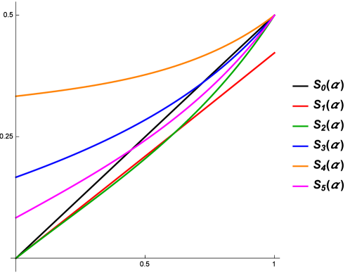
Figure 3: Graph of the optimal shift values $S_{0}(\alpha),S_{1}(\alpha)$, $S_{2}(\alpha),S_{3}(\alpha),S_{4}(\alpha)$ and $S_{5}(\alpha)$ of shifted approximations (6.55), (6.62), (6.78), (6.79), (6.80), (6.81).

Shifted approximations (6.78), (6.79), (6.80) and (6.81) have an order $2-\alpha$ when $y\in C^{2}[0,t_{n}]$ and $y(0)=y^{\prime}(0)=0$, and second order accuracy at their optimal shift values. The graphs of the optimal shift values $S_{0}(\alpha)$, $S_{1}(\alpha)$, $S_{2}(\alpha)$, $S_{3}(\alpha)$, $S_{4}(\alpha)$, $S_{5}(\alpha)$ of shifted approximations (6.55), (6.62), (6.78), (6.79), (6.80), (6.81) of the Caputo derivative, for $0<\alpha<1$, are given in Figure 3. The numerical results for the error and order of numerical solutions NS2(6.80) and NS2(6.81) of two-term equation (6.69) with $\alpha=0.3,m=7,s=0.25$, second order numerical solutions NS2(6.80) and NS2(6.80) of two-term equation (6.69) with $\alpha=0.6,m=4,s=S_{4}(0.6)=0.3926$ and $\alpha=0.5,m=5,s=S_{5}(0.5)=0.2428$ and numerical solutions NS3(6.80) and NS3(6.81) of order $2-2\alpha$ of three-term equation (6.73) with $\alpha=0.4,m=5,s=0.2$. are presented in Table 11 and Table 12.

7 Conclusions

In the present paper we derive approximations of the Caputo derivative and their asymptotic expansions related to the midpoint approximation of the integral in the definition of the Caputo derivative. The L1 approximation and approximation (1.15) of the Caputo derivative have an order $2-\alpha$ and properties (1) of the weights. According to the experimental results presented in the paper and the results from additional experiments with standard FDEs, approximation (1.15) has the advantage that the numerical solutions using (1.15) have smaller errors, which is explained with the smaller coefficient of the term of order ${2-\alpha}$ in the expansion formula and the smaller truncation error of the approximation. In section 6 we derive the induced shifted approximations, and their optimal shift values, of the Grunwald formula and the approximations of the Caputo derivative studied in the paper. A question for future work is to derive higher order shifted approximations of the Caputo derivative and to apply the approximations for numerical solution of ordinary and partial fractional differential equations.

8 Experimental results

The results of the numerical experiments are presented in Tables 1-12.

Table 1: Maximum error and order of numerical solution NS1(1.2) of order $2-\alpha$ of two-term equation (1.5) and $\alpha=0.25$, equation (1.6) and $\alpha=0.5$ and equation (1.7) with $\alpha=0.75$.

$\quad\boldsymbol{h}$	$\boldsymbol{\alpha=0.25}$		$\boldsymbol{\alpha=0.5}$		$\boldsymbol{\alpha=0.75}$
	$Error$	$Order$	$Error$	$Order$	$Error$	$Order$
$0.0125$	$0.4850\times 10^{-3}$	$1.6660$	$0.4009\times 10^{-3}$	$1.4695$	$0.1352\times 10^{-1}$	$1.2280$
$0.00625$	$0.1510\times 10^{-3}$	$1.6838$	$0.1438\times 10^{-3}$	$1.4792$	$0.5729\times 10^{-2}$	$1.2385$
$0.003125$	$0.4656\times 10^{-4}$	$1.6970$	$0.5134\times 10^{-4}$	$1.4857$	$0.2418\times 10^{-2}$	$1.2442$

Table 2: Maximum error and order of numerical solution NS1(2.27) of order $1-\alpha$ of two-term equation (1.5) and $\alpha=0.25$, equation (1.6) and $\alpha=0.5$ and equation (1.7) with $\alpha=0.75$.

$\quad\boldsymbol{h}$	$\boldsymbol{\alpha=0.25}$		$\boldsymbol{\alpha=0.5}$		$\boldsymbol{\alpha=0.75}$
	$Error$	$Order$	$Error$	$Order$	$Error$	$Order$
$0.0125$	$0.2132\times 10^{-1}$	$0.7606$	$0.5002\times 10^{-1}$	$0.5136$	$0.4984\times 10^{0}$	$0.3052$
$0.00625$	$0.1262\times 10^{-1}$	$0.7562$	$0.3514\times 10^{-1}$	$0.5096$	$0.4061\times 10^{0}$	$0.2955$
$0.003125$	$0.7486\times 10^{-2}$	$0.7536$	$0.2473\times 10^{-1}$	$0.5067$	$0.3324\times 10^{0}$	$0.2887$

Table 3: Maximum error and order of numerical solution NS1(3.34) of order $2-\alpha$ of two-term equation (1.5) and $\alpha=0.25$, equation (1.6) and $\alpha=0.5$ and equation (1.7) with $\alpha=0.75$.

$\quad\boldsymbol{h}$	$\boldsymbol{\alpha=0.25}$		$\boldsymbol{\alpha=0.5}$		$\boldsymbol{\alpha=0.75}$
	$Error$	$Order$	$Error$	$Order$	$Error$	$Order$
$0.0125$	$0.3891\times 10^{-3}$	$1.6940$	$0.3568\times 10^{-3}$	$1.4799$	$0.1298\times 10^{-1}$	$1.2334$
$0.00625$	$0.1192\times 10^{-3}$	$1.7064$	$0.1273\times 10^{-3}$	$1.4868$	$0.5489\times 10^{-2}$	$1.2414$
$0.003125$	$0.3631\times 10^{-4}$	$1.7152$	$0.4529\times 10^{-4}$	$1.4912$	$0.2314\times 10^{-2}$	$1.2460$

Table 4: Maximum error and order of second order numerical solution NS1(3.35) of two-term equation (1.5) and $\alpha=0.25$, equation (1.6) and $\alpha=0.5$ and equation (1.7) with $\alpha=0.75$.

$\quad\boldsymbol{h}$	$\boldsymbol{\alpha=0.25}$		$\boldsymbol{\alpha=0.5}$		$\boldsymbol{\alpha=0.75}$
	$Error$	$Order$	$Error$	$Order$	$Error$	$Order$
$0.0125$	$0.6259\times 10^{-4}$	$1.8774$	$0.2387\times 10^{-4}$	$1.9580$	$0.1878\times 10^{-2}$	$1.9220$
$0.00625$	$0.1642\times 10^{-4}$	$1.9310$	$0.6107\times 10^{-5}$	$1.9660$	$0.4825\times 10^{-3}$	$1.9605$
$0.003125$	$0.4218\times 10^{-5}$	$1.9602$	$0.1554\times 10^{-5}$	$1.9748$	$0.1225\times 10^{-3}$	$1.9781$

Table 5: Maximum error and order of numerical solution (4.37) of the fractional subdiffusion equation (4.39) at time $t=1$ for $\alpha=0.25,\alpha=0.5,\alpha=0.75$.

$\quad\boldsymbol{h}$	$\boldsymbol{\alpha=0.25}$		$\boldsymbol{\alpha=0.5}$		$\boldsymbol{\alpha=0.75}$
	$Error$	$Order$	$Error$	$Order$	$Error$	$Order$
$0.0125$	$0.2917\times 10^{-4}$	$1.7773$	$0.1514\times 10^{-3}$	$1.5084$	$0.7342\times 10^{-3}$	$1.2499$
$0.00625$	$0.8528\times 10^{-5}$	$1.7742$	$0.5328\times 10^{-4}$	$1.5067$	$0.3086\times 10^{-3}$	$1.2503$
$0.003125$	$0.2498\times 10^{-5}$	$1.7712$	$0.1877\times 10^{-4}$	$1.5053$	$0.1297\times 10^{-3}$	$1.2504$

Table 6: Maximum error and order of numerical solution (4.37) of the fractional subdiffusion equation (4.40) at time $t=1$ for $\alpha=0.25,\alpha=0.5,\alpha=0.75$.

$\quad\boldsymbol{h}$	$\boldsymbol{\alpha=0.25}$		$\boldsymbol{\alpha=0.5}$		$\boldsymbol{\alpha=0.75}$
	$Error$	$Order$	$Error$	$Order$	$Error$	$Order$
$0.0125$	$0.4063\times 10^{-3}$	$1.1216$	$0.8783\times 10^{-3}$	$1.0818$	$0.1641\times 10^{-2}$	$1.0661$
$0.00625$	$0.1942\times 10^{-3}$	$1.0652$	$0.4251\times 10^{-3}$	$1.0471$	$0.7947\times 10^{-3}$	$1.0453$
$0.003125$	$0.9483\times 10^{-4}$	$1.0339$	$0.2085\times 10^{-3}$	$1.0274$	$0.3884\times 10^{-3}$	$1.0327$

Table 7: Maximum error and order of numerical solution (4.37) of the fractional subdiffusion equation (4.41) at time $t=1$ for $\alpha=0.25$ and $m=8$, $\alpha=0.5$ and $m=4$ and $\alpha=0.75,m=2$.

$\quad\boldsymbol{h}$	$\boldsymbol{\alpha=0.25,m=8}$		$\boldsymbol{\alpha=0.5,m=4}$		$\boldsymbol{\alpha=0.75,m=2}$
	$Error$	$Order$	$Error$	$Order$	$Error$	$Order$
$0.0125$	$0.2484\times 10^{-4}$	$1.8641$	$0.9292\times 10^{-4}$	$1.5449$	$0.4714\times 10^{-3}$	$1.2690$
$0.00625$	$0.6842\times 10^{-5}$	$1.8534$	$0.3212\times 10^{-4}$	$1.5328$	$0.1966\times 10^{-3}$	$1.2615$
$0.003125$	$0.1916\times 10^{-5}$	$1.8431$	$0.1117\times 10^{-4}$	$1.5238$	$0.8228\times 10^{-4}$	$1.2570$

Table 8: Maximum error and order of second order numerical solution NS2(6.62) of equation (1.6) with $\alpha=0.3,s=0.25$, third order numerical solution NS2(6.62) of two-term equation (6.69) with $\alpha=0.6,m=5,s=S_{1}(0.6)=0.2523$ and second order numerical solution NS3(6.62) of three-term equation (6.73) with $\alpha=0.8,m=4,s=0.3$.

$\quad\boldsymbol{h}$	$\boldsymbol{\alpha=0.3,s=0.25}$		$\boldsymbol{\alpha=0.6,s=0.252}$		$\boldsymbol{\alpha=0.8,s=0.3}$
	$Error$	$Order$	$Error$	$Order$	$Error$	$Order$
$0.0125$	$0.1260\times 10^{-4}$	$2.0023$	$0.3703\times 10^{-7}$	$2.9815$	$0.3234\times 10^{-4}$	$1.9431$
$0.00625$	$0.3149\times 10^{-5}$	$2.0005$	$0.4656\times 10^{-8}$	$2.9916$	$0.8231\times 10^{-5}$	$1.9743$
$0.003125$	$0.7875\times 10^{-6}$	$1.9998$	$0.5835\times 10^{-9}$	$2.9961$	$0.2075\times 10^{-5}$	$1.9880$

Table 9: Maximum error and order of numerical solution NS2(6.78) of order $2-\alpha$ of two-term equation (6.69) with $\alpha=0.3,m=7,s=0.25$, second order numerical solution NS2(6.78) of two-term equation (6.69) with $\alpha=0.6,m=4,s=S_{2}(0.6)=0.2515$ and numerical solution NS3(6.78) of order $2-2\alpha$ of three-term equation (6.73) with $\alpha=0.4,m=6,s=0.2$.

$\quad\boldsymbol{h}$	$\boldsymbol{\alpha=0.3,s=0.25}$		$\boldsymbol{\alpha=0.6,s=0.251}$		$\boldsymbol{\alpha=0.4,s=0.2}$
	$Error$	$Order$	$Error$	$Order$	$Error$	$Order$
$0.0125$	$0.1444\times 10^{-4}$	$1.6669$	$0.1190\times 10^{-5}$	$1.8400$	$0.2769\times 10^{-3}$	$1.0590$
$0.00625$	$0.4523\times 10^{-5}$	$1.6747$	$0.3197\times 10^{-6}$	$1.8959$	$0.1252\times 10^{-3}$	$1.1458$
$0.003125$	$0.1411\times 10^{-5}$	$1.6801$	$0.8394\times 10^{-7}$	$1.9292$	$0.5552\times 10^{-4}$	$1.1727$

Table 10: Maximum error and order of numerical solution NS2(6.79) of order $2-\alpha$ of two-term equation (6.69) with $\alpha=0.3,m=7,s=0.25$, second order numerical solution NS2(6.79) of two-term equation (6.69) with $\alpha=0.6,m=4,s=S_{3}(0.6)=0.3164$ and numerical solution NS3(6.79) of order $2-2\alpha$ of three-term equation (6.73) with $\alpha=0.4,m=5,s=0.2$.

$\quad\boldsymbol{h}$	$\boldsymbol{\alpha=0.3,s=0.25}$		$\boldsymbol{\alpha=0.6,s=0.316}$		$\boldsymbol{\alpha=0.4,s=0.2}$
	$Error$	$Order$	$Error$	$Order$	$Error$	$Order$
$0.0125$	$0.4408\times 10^{-5}$	$1.8494$	$0.1652\times 10^{-5}$	$2.0178$	$0.3622\times 10^{-3}$	$1.1009$
$0.00625$	$0.1233\times 10^{-5}$	$1.8379$	$0.4093\times 10^{-6}$	$2.0126$	$0.1608\times 10^{-3}$	$1.1716$
$0.003125$	$0.3482\times 10^{-6}$	$1.8244$	$0.1017\times 10^{-6}$	$2.0083$	$0.7030\times 10^{-4}$	$1.1938$

Table 11: Maximum error and order of numerical solution NS2(6.80) of order $2-\alpha$ of two-term equation (6.69) with $\alpha=0.3,m=7,s=0.25$, second order numerical solution NS2(6.80) of two-term equation (6.69) with $\alpha=0.6,m=4,s=S_{4}(0.6)=0.3926$ and numerical solution NS3(6.80) of order $2-2\alpha$ of three-term equation (6.73) with $\alpha=0.4,m=5,s=0.2$.

$\quad\boldsymbol{h}$	$\boldsymbol{\alpha=0.3,s=0.25}$		$\boldsymbol{\alpha=0.6,s=0.393}$		$\boldsymbol{\alpha=0.4,s=0.2}$
	$Error$	$Order$	$Error$	$Order$	$Error$	$Order$
$0.0125$	$0.6032\times 10^{-5}$	$1.3520$	$0.4187\times 10^{-5}$	$1.9825$	$0.4543\times 10^{-3}$	$1.1289$
$0.00625$	$0.2183\times 10^{-5}$	$1.4663$	$0.1055\times 10^{-5}$	$1.9881$	$0.1993\times 10^{-3}$	$1.1892$
$0.003125$	$0.7540\times 10^{-6}$	$1.5337$	$0.2655\times 10^{-6}$	$1.9912$	$0.8623\times 10^{-4}$	$1.2084$

Table 12: Maximum error and order of numerical solution NS2(6.81) of order $2-\alpha$ of two-term equation (6.69) with $\alpha=0.3,m=7,s=0.25$, second order numerical solution NS2(6.81) of two-term equation (6.69) with $\alpha=0.5,m=5,s=S_{5}(0.5)=0.2428$ and numerical solution NS3(6.81) of order $2-2\alpha$ of three-term equation (6.73) and $\alpha=0.4,m=6,s=0.2$.

$\quad\boldsymbol{h}$	$\boldsymbol{\alpha=0.3,s=0.25}$		$\boldsymbol{\alpha=0.5,s=0.243}$		$\boldsymbol{\alpha=0.4,s=0.2}$
	$Error$	$Order$	$Error$	$Order$	$Error$	$Order$
$0.0125$	$0.9541\times 10^{-5}$	$1.1714$	$0.6344\times 10^{-6}$	$2.0819$	$0.3177\times 10^{-3}$	$1.0815$
$0.00625$	$0.2914\times 10^{-5}$	$1.7111$	$0.1528\times 10^{-6}$	$2.0536$	$0.1422\times 10^{-3}$	$1.1597$
$0.003125$	$0.8909\times 10^{-6}$	$1.7097$	$0.3730\times 10^{-7}$	$2.0344$	$0.6258\times 10^{-4}$	$1.1841$

¹ Department of Mathematics and Physics
University of Forestry
10 Sveti Kliment Ohridski Blv.,
Sofia – 1756, BULGARIA
e-mail: yuri.dimitrov@ltu.bg Received: September 1, 2018
² Institute of Mathematics and Informatics,
Bulgarian Academy of Sciences,
Department of Information Modeling, Acad. Georgi Bonchev Str., Block 8,
Sofia – 1113, BULGARIA
vtodorov@math.bas.bg
² Institute of Information and Communication Technologies,
Bulgarian Academy of Sciences,
Department of Parallel Algorithms, Acad. Georgi Bonchev Str., Block 25A,
Sofia – 1113, BULGARIA
venelin@parallel.bas.bg
³ Department of Statistics and Applied Mathematics
University of Economics
77 Knyaz Boris I Blvd.,
Varna – 9002, BULGARIA
e-mail: miryanov@ue-varna.bg

References

• [1] J. H. Ahlberg, E. N. Nilson, Convergence properties of the spline fit. J. Soc. Ind. Appl. Math. 11, No 1 (1963), 95–104.
• [2] A. A. Alikhanov, A new difference scheme for the time fractional diffusion equation. J. Comput. Phys. 280 (2015), 424–438.
• [3] M. Chen, W. Deng, A second-order numerical method for two-dimensional two-sided space fractional convection diffusion equation. Appl. Math. Model. 38, No 13 (2014), 3244–3259.
• [4] K. Diethelm, The Analysis of Fractional Differential Equations: An Application-Oriented Exposition Using Differential Operators of Caputo Type. Springer (2010).
• [5] K. Diethelm, S. Siegmund, H. T. Tuan, Asymptotic behavior of solutions of linear multi-order fractional differential systems. Fract. Calc. Appl. Anal. 20, No 5 (2017), 1165–1195; DOI: 10.1515/fca-2017-0062;
• [6] Y. Dimitrov, Numerical approximations for fractional differential equations. J. Fract. Calc. Appl. 5, No 3S (2014) 1–45.
• [7] Y. Dimitrov, A second order approximation for the Caputo fractional derivative. J. Fract. Calc. Appl. 7, No 2 (2016), 175–195.
• [8] Y. Dimitrov, Three-point approximation for the Caputo fractional derivative. Communication on Applied Mathematics and Computation 31, No 4 (2017), 413–442.
• [9] Y. Dimitrov, Approximations for the Caputo derivative (I). J. Fract. Calc. Appl 9, No 1 (2018), 35–63.
• [10] Y. Dimitrov, R. Miryanov, V. Todorov, Asymptotic expansions and approximations of the Caputo Derivative. Comp. Appl. Math. (2018); DOI: 10.1007/s40314-018-0641-3;
• [11] Y. Dimitrov, I. Dimov, V. Todorov, Numerical solutions of ordinary fractional differential equations with singularities. In: Advanced Computing in Industrial Mathematics (2018); DOI:10.1007/978-3-319-97277-0.
• [12] H. Ding, C. Li, High-order algorithms for Riesz derivative and their applications (III). Fract. Calc. Appl. Anal. 19, No 1 (2016), 19–55; DOI: 10.1515/fca-2016-0003;
• [13] H. Ding, C. Li, High-order numerical algorithms for Riesz derivatives via constructing new generating functions. J. Sci. Comput. 71, No 2 (2017), 759–784.
• [14] N. ElezoviΔ‡ Asymptotic expansions of gamma and related functions, binomial coefficients, inequalities and means. J. Math. Inequal. 9, No 4 (2005), 1001–1054.
• [15] G. H. Gao, Z. Z. Sun, H. W. Zhang, A new fractional numerical differentiation formula to approximate the Caputo fractional derivative and its applications. J. Comput. Phys. 259 (2014), 33–50.
• [16] C.-C. Ji, Z.-Z. Sun, A high-order compact finite difference scheme for the fractional sub-diffusion equation. J. Sci. Comput. 64, No 3 (2015), 959–985.
• [17] S. Jiang, J. Zhang, Q. Zhang, Z. Zhang, Fast evaluation of the Caputo fractional derivative and its applications to fractional diffusion equations. Commun. Comput. Phys. 21, No 3 (2017), 650–678.
• [18] B. Jin, R. Lazarov, Z. Zhou, An analysis of the L1 scheme for the subdiffusion equation with nonsmooth data. IMA J. Numer. Anal. 36, No 1 (2016), 197–221.
• [19] K. Kumar, R. K. Pandey, S. Sharma, Approximations of fractional integrals and Caputo derivatives with application in solving Abel’s integral equations. JKSUS (2018); DOI: 10.1016/j.jksus.2017.12.017.
• [20] C. Li, A. Chen, J. Ye, Numerical approaches to fractional calculus and fractional ordinary differential equation. J. Comput. Phys. 230, No 9 (2011), 3352–3368.
• [21] H. Li, J. Cao, C. Li, High-order approximation to Caputo derivatives and Caputo-type advection–diffusion equations (III). J. Comput. Appl. Math. 299 (2016). 159–175.
• [22] Y. Lin, C. Xu, Finite difference/spectral approximations for the time-fractional diffusion equation. J. Comput. Phys. 225, No 2 (2007), 1533–1552.
• [23] C. Li, F. Zeng, Numerical methods for fractional calculus. Chapman and Hall/CRC (2015).
• [24] Y. Ma, Two implicit finite difference methods for time fractional diffusion equation with source term. Journal of Applied Mathematics and Bioinformatics. 4, No 2 (2014), 125–145.
• [25] Z. Odibat, Approximations of fractional integrals and Caputo fractional derivatives. Appl. Math. Comput. 178, No 2 (2006), 527–533.
• [26] I. Podlubny, Fractional Differential Equations. Academic Press, San Diego (1999).
• [27] J. Ren, S. Mao, J. Zhang, Fast evaluation and high accuracy finite element approximation for the time fractional subdiffusion equation. Numer. Methods Partial Differ. Equ. 34, No 2 (2018), 705–730.
• [28] L. Ren, Y. M. Wang, A fourth-order extrapolated compact difference method for time-fractional convection-reaction-diffusion equations with spatially variable coefficients. Appl. Math. Comput. 312 (2017), 1–22.
• [29] Z.-Z. Sun, X. Wu, A fully discrete scheme for a diffusion wave system. Appl. Numer. Math. 56, No 2 (2006), 193–209.
• [30] E. Sousa, A second order explicit finite difference method for the fractional advection diffusion equation. Comput. Math. Appl. 64, No 10 (2012), 3141–3152.
• [31] C. Tadjeran, M. M. Meerschaert, H. P. Scheffer, A second-order accurate numerical approximation for the fractional diffusion equation. J. Comput. Phys. 213 (2006), 205–213.
• [32] W. Tian, H. Zhou, W. Deng, A class of second order difference approximation for solving space fractional diffusion equations, Math. Comput. 84 (2015), 1703–1727.
• [33] F. Tricomi, A. ErdΓ©lyi, The asymptotic expansion of a ratio of gamma functions. Pac. J. Math.. 1, No 1 (1951), 133–142.
• [34] J. M. Varah, A lower bound for the smallest singular value of a matrix. Linear Algebra Appl. 11, No 1 (1975), 3–5.
• [35] Z. Wang, S. Vong, Compact difference schemes for the modified anomalous fractional sub-diffusion equation and the fractional diffusion-wave equation. J. Comput. Phys. 277 (2014), 1–15.
• [36] W. Wyss, The fractional diffusion equation. J. Math. Phys. 27, (1986); https://doi.org/10.1063/1.527251
• [37] Y. Yan, K. Pal, N. J. Ford, Higher order numerical methods for solving fractional differential equations. BIT Numer. Math. 54, No 2 (2014), 555–584.
• [38] Y. Yan, Z.-Z. Sun, J. Zhang, Fast evaluation of the Caputo fractional derivative and its applications to fractional diffusion equations: A second-order scheme. Commun. Comput. Phys. 22, No 4 (2017), 1028–1048.
• [39] F. Zeng, C. Li, F. Liu, I. Turner, Numerical algorithms for time-fractional subdiffusion equation with second-order accuracy. SIAM J. Sci. Comput. 37, No 1 (2015), A55–A78.
• [40] F. Zeng, Z. Zhang, G. E. Karniadakis, Second-order numerical methods for multi-term fractional differential equations: Smooth and non-smooth solutions. Comput. Methods Appl. Mech. Eng. 327 (2017), 478–502.