Extreme-scale Multigrid Components within PETSc

Abstract

Elliptic partial differential equations (PDEs) frequently arise in continuum descriptions of physical processes relevant to science and engineering. Multilevel preconditioners represent a family of scalable techniques for solving discrete PDEs of this type and thus are the method of choice for high-resolution simulations. The scalability and time-to-solution of massively parallel multilevel preconditioners can be adversely effected by using a coarse-level solver with sub-optimal algorithmic complexity. To maintain scalability, agglomeration techniques applied to the coarse level have been shown to be necessary.

In this work, we present a new software component introduced within the Portable Extensible Toolkit for Scientific computation (PETSc) which permits agglomeration. We provide an overview of the design and implementation of this functionality, together with several use cases highlighting the benefits of agglomeration. Lastly, we demonstrate via numerical experiments employing geometric multigrid with structured meshes, the flexibility and performance gains possible using our MPI-rank agglomeration implementation.

1 Introduction

In numerous branches of computational science and engineering, there is frequently a need to solve large systems of linear equations of the form

(1) $$\mathbf{A}\mathbf{x}=\mathbf{b},\quad\mathbf{A}\in\mathbb{R}^{n\times n},\quad\mathbf{x},\mathbf{b}\in\mathbb{R}^{n}$$

which arise from the spatial discretization of partial differential equations (PDEs) which contain scalar (or vectorial) elliptic operators. Examples include, but are not limited to: steady-state thermal conduction

(2) $$-\nabla\cdot\bigl{(}k\nabla\phi\bigr{)}=f,$$

where $k$ is the thermal conductivity and $\phi$ is the temperature; displacement $(\boldsymbol{u})$ formulations of small-strain elastostatics

(3) $$-\nabla\cdot\bigl{(}\bar{\boldsymbol{C}}\,\epsilon[\boldsymbol{u}]\bigr{)}=\boldsymbol{g},$$

where $\epsilon[\boldsymbol{x}]=\tfrac{1}{2}\left(\nabla\boldsymbol{x}+(\nabla\boldsymbol{x})^{T}\right)$ is the symmetric gradient of a vector and $\bar{\boldsymbol{C}}$ is the constitutive tensor; and stationary incompressible Stokes flow

(4) $$-\nabla\cdot\bigl{(}2\eta\,{\epsilon}[\boldsymbol{v}]\bigr{)}+\nabla p=\boldsymbol{h},\quad-\nabla\cdot\boldsymbol{v}=0,$$

where $\boldsymbol{v},p$ is the velocity and pressure, respectively, and $\eta$ is the viscosity of the fluid.

Given the wide-spread availability of massively parallel, distributed memory computing capabilities offered by computing centres, application scientists continue to push the boundaries of both (i) simulation spatio-temporal resolution, and (ii) simulation throughput. In the context of simulation resolution, leadership computing facilities provide resources which, if used at full capacity, can theoretically enable 3D simulations to be performed with billions or trillions of unknowns $(n)$ [8]. Alternatively, for a given spatio-temporal resolution, simulation throughput, or time-to-solution, can be accelerated by using more compute resources. Whilst the algorithmic demands in the weak scaling limit (resolution) or strong scaling limit (throughput) are different, the most time-consuming part of application software which involve discretized elliptic operators invariably is associated with the solution of Eq. (1).

Preconditioned Krylov (iterative) methods are desirable solution algorithms in massively parallel computing environments as their fundamental building blocks, e.g. matrix-vector products, norms, and dot products, readily map to distributed memory implementations. Nevertheless, without a suitable preconditioner, the number of iterations required by a Krylov method will rapidly increase under spatial refinement when applied to discrete elliptic operators. To accelerate the convergence of Krylov methods, multilevel preconditioners such as those derived from two-level domain-decomposition methods (e.g. additive Schwarz), algebraic multigrid, or geometric multigrid are preferred choices. These methods represent a family of efficient and scalable techniques for solving elliptic PDEs by eliminating errors across all scales through a hierarchy of coarse meshes, or coarse subspaces. Selecting the particular multilevel preconditioner is dependent on both the characteristic of the physical problem (e.g. the nature of the coefficient in the elliptic operator) and specific details related to the spatial discretization (e.g. structured mesh versus unstructured, low order basis versus high order basis functions). When geometric multigrid is a viable option, it will generally be more efficient than an algebraic multigrid implementation due to (i) a scalable setup phase, (ii) the possibility to use highly optimized matrix-free smoothers on all levels, and (iii) the ability to utilize an identical stencil (non-zero structure) throughout all coarse-level operators. In this work, we are primarily concerned with multilevel preconditioners which utilize geometric information (such as a mesh) and thus we will focus the remainder of this discussion on such techniques.

Geometric multigrid with re-discretized operators is the most common form of multilevel preconditioner used to solve elliptic problems when a hierarchy of successively refined meshes, and the interpolation and prolongation operations between them is readily available. The reason why multigrid is undoubtedly the preconditioner of choice for elliptic problems is because the method is both algorithmically scalable (e.g. converges in a fixed number of iterations independent of the mesh resolution) and optimal. That is, for a given solution accuracy, the time-to-solution is proportional to the number of unknowns $n$, as are the storage requirements of the method. This is in contrast to, for example, sparse direct methods which have a time-to-solution which scales like $O(n^{3/2})$ (2D) or $O(n^{2})$ (3D) [14]. The sequential multigrid preconditioner obtains its $O(n)$ behaviour as the amount of work to be performed on each level $k=1,\dots,N$ (except the coarsest) is proportional to $n_{k}$. In the case of a three-dimensional problem with a coarsening factor of 2, the work per level decreases by a factor of $8$. On the coarsest level $(k=1)$ it is traditionally advocated to utilize an exact LU factorization. Despite the $O(n_{1}^{2})$ scaling for the factorization, $n_{1}$ on the coarse level will contain $1/8^{N-1}$ times fewer unknowns than the finest level and thus the cost of the direct solve is negligible.

The treatment of coarse levels within the geometric multigrid hierarchy in a massively parallel distributed memory setting requires some consideration as the ratio between communication and computation becomes larger with each coarser level. Thus, the time spent on each level is not guaranteed to be a factor of $1/8$ times less than the next finest level. Moreover, the cost of performing an exact LU factorization of a very small problem distributed over many MPI-ranks may no longer be negligible. Several strategies have been proposed to treat coarse-level solves in multigrid preconditioners [28]:

1. Truncate the number of multigrid levels when the cost of the communication cannot be overlapped with the computation on a given level, or when there is less than one unknown per MPI-rank. The depth of the multigrid hierarchy might be shallower than the equivalent sequential hierarchy, and thus an iterative solver on the “coarsest” level should be used. In practice it is observed that an inexact coarse-level solve up to a specified tolerance can yield an optimal multigrid preconditioner [16, 28]. However, the cost of obtaining a fixed-precision inexact solve could be $n_{k}\log n_{k}$ and given the shallow nature of the hierarchy, this cost may be sufficient to degrade the expected $O(n)$ time-to-solution.

2. Allow for a subset of MPI-ranks to have zero unknowns, thereby introducing idle processing units.

3. Agglomerate unknowns onto a new MPI communicator with fewer ranks. That is, coarsen the size of the MPI communicator in conjunction with the mesh coarsening to provide a more favourable balance between communication and computation. This concept is illustrated in Fig. 1.

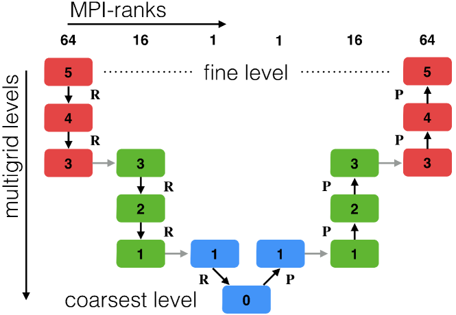
Figure 1: Multigrid V-cycle with agglomeration. $\mathbf{R}$ and $\mathbf{P}$ denote the restriction and prolongation operators respectively. Grey horizontal arrows indicate where agglomeration occurs and data is moved between different communicators.

In practice, selecting the ideal coarse-level solver strategy is very much problem-dependent (e.g. constant coefficient versus spatially heterogenous) and machine-dependent (e.g. the latency associated of the network and the cost of global reductions versus floating point speed).

There are numerous examples in the literature where the three different coarse-level solver strategies have been adopted. The truncation strategy is most frequently adopted. It is the simplest to implement as only the finest level is required to be partitioned over a single MPI communicator. In [8, 9, 10] the effect of using the conjugate gradient method as a coarse-level solver and its influence on the parallel scalability of multigrid was examined. On large-scale computations employing more than 100k processing cores, the cost of the coarse-level solve represented $\sim$15% of the total compute time. Hierarchical Krylov methods [17] were utilized as the coarse level solver in [16] to reduce the number of global reductions required, and thereby providing a better balance between communication and computation.

In [1, 27], a fixed size MPI communicator was used across all levels and the number of active processors was reduced by completely eliminating unknowns from some MPI-ranks. A detailed examination of the performance gains of using this approach was not discussed by either author. The downside of introducing “zero work ranks” is twofold. Firstly, if any collective calls are used, all ranks must participate in the operation. Secondly, this programming model lacks generality beyond its applicability for linear algebra objects such as matrices and vectors. Using different MPI communicators is the correct paradigm to adopt and thus it naturally works with all parallel objects. Thus, agglomeration employing separate communicators is preferable in a general framework.

Various implementations of process agglomeration have been utilized within the solver community, e.g. [5, 7, 16, 18, 19, 21]. In general, the agglomeration methods require a-priori specification of when agglomeration should occur and how aggressive it should be. However, based on most published results, there appears to be a lack of a performance model to guide such choices. Instead, experimentation is used to determine the minimum time-to-solution. Consequently, the true benefits of using agglomeration are not clearly characterized or examined in detail in most studies. We note that this may in part be due to the problem- and machine-dependent nature of the scalability issues connected with coarse-level solvers. For a range of problems containing less than about $3$M unknowns and scaling using up to 32 cores, a comparison of using a parallel LU factorization, an iterative method, and an agglomeration strategy together with algebraic multigrid has indicated that agglomeration is a superior approach [7]. For medium-sized problems containing approximately $25$M unknowns on 4096 cores, the benefits of using agglomeration compared to an iterative coarse-level solver combined with smoothed aggregation algebraic multigrid on 4096 cores was demonstrated in [16], with an overall solver speed-up of 1.8 being reported. For large-scale computations using the UG framework [19] with problem sizes in excessive of 1B unknowns, agglomeration was found essential to obtain good scalability past 4096 cores. In the example presented, solve times were a factor of 1.8 faster than those without agglomeration.

1.1 Contributions

In this work, we describe a newly developed component within the Portable Extensible Toolkit for Scientific computation (PETSc) [2, 3, 4] which permits agglomeration. Rather than develop a new multigrid implementation which supports agglomeration, we developed a flexible and re-usable component which can be utilized in a multitude of different ways. The agglomeration operation is exposed within a new preconditioner object and as such can be readily composed with all other existing non-linear solvers, linear solvers, and preconditioner objects within PETSc. Unique to the agglomeration implementation we describe here is that it utilizes geometric information which may have been attached to the outer Krylov method. Therefore, it can be seamlessly used together with domain-decomposition and multigrid-type preconditioners. The details pertaining to the design and implementation of the agglomeration preconditioner within PETSc is discussed, together with a number of typical use cases where this methodology can be beneficial. Lastly, we present several numerical experiments employing geometric multigrid to highlight both the flexibility of the proposed preconditioner, and the performance gains possible through MPI-rank agglomeration.

2 Solvers and Discretization Components in PETSc

2.1 Preconditioned Krylov Subspace Methods

Stationary, fixed-point iterative methods and preconditioned Krylov subspace methods within PETSc are defined by the KSP abstract class. The KSP object provides a rich family of iterative methods such as Richardson, Chebyshev (fixed point); CG, GMRES (Krylov); GCR, FGMRES (flexible Krylov methods); and pipelined variants of CG and GMRES.

Essential to the convergence of Krylov methods is the choice of a preconditioner. PETSc provides a large number of preconditioners via the PC class. This includes classical methods such as Jacobi, incomplete LU factorization (ILU), successive over-relaxation (SOR), block-Jacobi; domain decomposition methods such as additive Schwarz (ASM), balancing Neumann-Neumann (NN), balancing domain decomposition by constraints (BDDC); multilevel methods such as smoothed aggregation algebraic multigrid (GAMG); and a method for “block” or “physics-based” preconditioners (FieldSplit).

A fundamental design choice within PETSc is that solvers and preconditioners can be configured at run-time. The degree of configurability ranges from generic solver parameters (e.g. tolerances for stopping conditions), to the specific Krylov method and the type of preconditioner used. Moreover, solvers and preconditioner objects readily can be composed with each other at run-time using command line arguments (or an input file consisting of a set of command line arguments). Configuration and composability of nested solvers and preconditioners is enabled through the implementations assigning names (prefixes) to any internal KSP or PC objects. These prefixes are concatenated together to provide unique textual identifiers for each configurable parameter which can be defined at run-time. This mechanism allows end users to switch, at run-time, between a simple, non-scalable solver to a highly sophisticated, scalable method without changing a single line of code in their application software . For example, given an assembled matrix, users can either select to use CG with block-Jacobi and employ ILU on each sub-domain, or they can select to use CG with algebraic multigrid.

The degree of composability supports the end users’ diverse and ever-changing requirements. A priori, the end user is unlikely to know the optimal solver and preconditioner configuration they will require. The choice of the “optimal preconditioner” is dependent on many factors. For instance, assuming the matrix is associated with a discretization of a PDE, influencing factors may include (but not exclusively): the characteristics of the underlying PDE (e.g. elliptic versus parabolic), the nature of the coefficients in the PDE (e.g. constant, smooth, discontinuous), the type of boundary conditions (e.g. Dirichlet versus Neumann), the type of discretization, etc. Changing any of these factors within the application software will invariably mandate changing the solver and preconditioner configuration in order to preserve the “optimal” choice.

2.1.1 Multigrid

To introduce the base multigrid implementation in PETSc (PCMG), we begin by first summarizing the classic two-level multigrid algorithm in Alg. 1 as applied to Eq. (1).

Algorithm 1 Two-level Multigrid

1:Given $\mathbf{A}$, $\mathbf{M}$, $\mathbf{R}$, $\mathbf{P}$, $\mathbf{A}_{c}$, $\mathbf{b}$

2:Choose ${\mathbf{u}}^{0}$

3:repeat

4:   ${\mathbf{u}}^{i}\leftarrow{\mathbf{u}}^{i}+{\mathbf{M}}^{-1}\,({\mathbf{b}}-\mathbf{A}\mathbf{u}^{i})$ $\triangleright$ pre-smooth $m$ times

5:   ${\mathbf{r}}={\mathbf{R}}\,({\mathbf{b}}-\mathbf{A}\mathbf{u}^{i})$ $\triangleright$ restrict residual

6:   ${\mathbf{A}_{c}}\,{\mathbf{e}}={\mathbf{r}}$ $\triangleright$ solve for coarse grid correction

7:   ${\mathbf{u}}^{i}\leftarrow{\mathbf{u}}^{i}+{\mathbf{P}}\,{\mathbf{e}}$ $\triangleright$ prolongate error

8:   ${\mathbf{u}}^{i}\leftarrow{\mathbf{u}}^{i}+{\mathbf{M}}^{-1}({\mathbf{b}}-{\mathbf{A}}\,{\mathbf{u}}^{i})$ $\triangleright$ post-smooth $m$ times

9:   ${\mathbf{u}}^{i+1}\leftarrow{\mathbf{u}}^{i}$ $\triangleright$ update for next iteration

10:until converged

A multigrid algorithm defines a hierarchy of levels – with the top and bottom being referred to as “fine” and “coarse”, respectively. On each level (except the coarsest), we require (i) an operator $\mathbf{A}$, and an operator used for preconditioning $\mathbf{M}$, (ii) a “smoother”, (iii) an operator to restrict a solution vector to the next coarsest level ($\mathbf{R}$), and (iv) an operator to prolongate a solution vector from the coarse level below ($\mathbf{P}$). On the coarsest level in the hierarchy we require a “coarse” level solver. In the context of classical geometric multigrid, the “smoother” typically defines a fixed point iterative method which, when applied to a vector, removes high frequency error components, whilst the coarse-level solver is generally taken to be an LU factorization (exact solve). In PCMG, both the smoother and the coarse-level solver are defined as KSP objects. As such, they can be configured to define a fixed-point method such as Richardson - Jacobi (classical smoother), or an exact solver. To enable different run-time configuration of the KSP on coarsest level and all other levels, the option prefix -mg_coarse and -mg_levels is used.

2.2 Distribution Manager

Solvers based purely on provided matrix entries are limited in their ability to perform well since one cannot take advantage of geometric or modeling information. Hence, a solver framework that allows access to this information is vital. The difficulty is creating a flexible, hierarchical way to provide this information that is nonintrusive, yet powerful. One unique feature of PETSc is the Distribution Manager (DM) abstract class, which provides information to the algebraic solvers regarding the mesh and physics but does not impose constraints on their management. We emphasize that DM is not a mesh management class and does not provide an interface to low-level mesh functionality; rather, DM provides an interface for accessing information relevant to and needed by the solver. To that end, the DM class in PETSc provides a high-level interface for obtaining mesh information to the solver.

A DM encodes two linear spaces, the global space which encompasses the entire problem (e.g. as required to store the solution of a PDE) which is appropriate for global solves, and the local space composed of overlapping, or ghosted, subspaces appropriate for local function evaluations. The DM can create a vector from either space, and also a properly preallocated matrix from the global space. In addition, it can provide a mapping between the global representation of a field and its local representation, or vice versa.

The DM also establishes a natural notion of hierarchy. The user can obtain a refined or coarsened version of the DM, along with operators mapping fields between these spaces. While for structured grids (DMDA) these operations can be defined solely in PETSc, for unstructured grids (DMPlex) we use third party mesh manipulation packages such as Pragmatic [20], Triangle [24, 23], and TetGen [25, 26] to produce refined and coarsened meshes.

In addition to the hierarchy, the DM has an interface for creating subspaces. It provides a consistent naming and representation of sub-fields of the global field using index sets, or IS objects. By representing subspaces as simple sets of integers, interaction with the solvers and linear algebra methods is simple and clean. A restriction operation is provided onto the subspace, whether it be a subset of the fields or a subset of the domain. In fact, a sub-DM can be created for the subspace, so the full problems can be solved consistently.

A DM can also be attached to a Krylov method and its preconditioner. Several preconditioner implementations in PETSc are “DM aware” and can use these objects in implementation specific manners. For example, the additive Schwarz preconditioner can use an attached DM to define overlapping sub-domains. Similarly, PCMG can use an attached DM to define both a mesh hierarchy through coarsening, and the restriction and prolongation operators between each mesh level.

3 Design & Implementation of Telescope

3.1 Design Considerations

The DM class currently does not provide support for repartitioning. Even if it did, integrating repartitioning within the multigrid framework would be awkward, and the resulting functionality could not be directly used with other solver components. We decided that a more natural and re-usable way to introduce repartitioning into the composable solver space provided by PETSc is to embed this functionality within a new preconditioner implementation – we call this implementation Telescope.

The general definition of a preconditioner in PETSc is the operation $\mathbf{y}=\mathbf{A}^{-1}\mathbf{x}$. From this, the essential philosophy behind Telescope is summarized below:

1. Given an MPI communicator $\mathcal{C}$, create a new communicator $\mathcal{C}^{\prime}$.

2. Repartition the input matrix $\mathbf{A}$ and vector $\mathbf{x}$ onto $\mathcal{C}^{\prime}$, yielding $\mathbf{A}^{\prime}$ and $\mathbf{x}^{\prime}$.

3. Apply a Krylov method to solve $\mathbf{A}^{\prime}\mathbf{y}^{\prime}=\mathbf{x}^{\prime}$ on $\mathcal{C}^{\prime}$.

4. Scatter the solution $\mathbf{y}^{\prime}$ to $\mathcal{C}$ to obtain $\mathbf{y}$.

The notion of using a “preconditioner” as an entry point to enable repartitioning or modification of a matrix is utilized in the existing PETSc preconditioners Redundant and Redistribute already.

The size (number of MPI-ranks) of the communicator $\mathcal{C}^{\prime}$, denoted by $n_{\mathcal{C}^{\prime}}$, is defined by $n_{\mathcal{C}}/r$, where $r$ is the rank reduction factor specified by the user. A subset of MPI-ranks from $\mathcal{C}$ are used to define $\mathcal{C}^{\prime}$. Denoting the index of each MPI-rank in $\mathcal{C}$ via $R_{\mathcal{C}}^{k}\in[0,n_{\mathcal{C}}-1]$, any index for which $\text{mod}(R_{\mathcal{C}}^{k},r)$ equals zero is included within $\mathcal{C}^{\prime}$. The strided layout of MPI-ranks in $\mathcal{C}^{\prime}$ is advantageous when the available RAM per-core is limited and thus distributing the repartitioned objects $\mathbf{A}^{\prime},\mathbf{x}^{\prime}$ over more compute nodes is desirable. MPI-ranks in $\mathcal{C}$ which are not used within $\mathcal{C}^{\prime}$ are idle during the application of the nested Krylov method. We argue that this choice is both more efficient and simpler to implement than an alternative implementation which performs redundant calculations.

We note that objects defined on both communicators $\mathcal{C}$ and $\mathcal{C}^{\prime}$ (e.g. $\mathbf{A},\mathbf{x},\mathbf{y}$) are held in memory.

3.2 Special Cases

Here we describe the different features of the implementation of Telescope which will allude to its potential usage within the context of multilevel and domain decomposition preconditioners, and highlight the differences with the related preconditioner Redundant.

• In PETSc, a sparse matrix with communicator $\mathcal{C}$ will be partitioned across all MPI-ranks using a row-wise decomposition, e.g.  $\mathbf{A}=[\mathbf{A}_{0};\,\mathbf{A}_{1};\,\dots;\,\mathbf{A}_{n_{\mathcal{C}}-1}]$. When Telescope is provided with $\mathbf{A}$ and a DM has not been attached to the preconditioner, the repartitioned matrix $\mathbf{A}^{\prime}$ is constructed by contiguously fusing rows of $\mathbf{A}$ such that $\mathbf{A}^{\prime}=[\mathbf{A}^{\prime}_{0};\,\dots;\,\mathbf{A}^{\prime}_{n_{\mathcal{C}^{\prime}}-1}]$ where

  $$\mathbf{A}^{\prime}_{k}=\big{[}\mathbf{A}_{kr};\,\mathbf{A}_{kr+1};\,\dots;\,\mathbf{A}_{kr+r-1}\big{]},$$

  $k$ is the index of an MPI-rank within $\mathcal{C}^{\prime}$ and $r$ is the user-specified rank reduction factor. The redistribution of $\mathbf{A}$ occurs in two phases which are depicted in Fig. 2b), c). The intermediate matrices $\mathbf{A}^{r}_{k}$ are sequential objects that are formed through a combination of copying local data from the same rank (blue arrows) and scattering data from ranks being agglomerated (red arrows). The operator $\mathbf{A}^{\prime}$ is identical to that which would be defined using Redundant, with the exception, that it is only defined on a subset of MPI-ranks within the parent communicator ${\mathcal{C}}$ and no redundant work is performed on the other MPI-ranks.

  

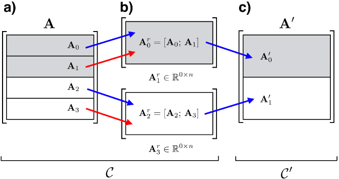
  Figure 2: Matrix redistribution: a) Original matrix defined on $\mathcal{C}$; b) Intermediate sequential matrices on all ranks in $\mathcal{C}$. Ranks not in $\mathcal{C}^{\prime}$ contain zero rows; c) Redistributed matrix defined on the reduced communicator $\mathcal{C}^{\prime}$.

• PETSc provides two mechanisms to remove null spaces from an operator. The user can provide either (or both): a set of $n_{s}$ vectors $\boldsymbol{\phi}_{i}$ representing each null space, or a function which will perform the removal. If the original operator $\mathbf{A}$ has a null space attached, the vectors $\boldsymbol{\phi}_{i}$ are scattered onto $\mathcal{C}^{\prime}$ and attached to $\mathbf{A}^{\prime}$. Any user-provided null space removal function attached to $\mathbf{A}$ is also assigned to the null space defined on $\mathbf{A}^{\prime}$. Redundant currently does not support propagation of the null space to the repartitioned matrix.

• To support scalable multilevel algorithms, Telescope exploits geometric and discretization information which is provided by an attached DM defined on $\mathcal{C}$. We denote by $\mathcal{T}$ the discretization defined by the DM. An exact definition of $\mathcal{T}$ cannot be provided as it depends on the type of the DM, but it should be regarded as representing: geometric primitives (e.g. points, edges, faces, cells); topological relationships between the geometric primitives; geometry (e.g. coordinates); and field information (e.g. number of degrees of freedom attached to each geometric primitive). For example, in the case of a DMDA (structured grid), $\mathcal{T}$ defines the number of grid points in each $i,j,k$ direction in both the local and global space, and the coordinates of each grid point. Due to the structured nature of the DMDA, $\mathcal{T}$ also implicitly defines the ordering of unknowns and the connectivity between each grid point.

  When a DM is provided, $\mathcal{T}$ is repartitioned onto $\mathcal{C}^{\prime}$, resulting in $\mathcal{T}^{\prime}$. The redistribution phase of $\mathbf{A}$ and $\mathbf{x}$ must preserve the re-ordering of the unknowns which occurred when $\mathcal{T}$ was repartitioned.

  Currently, Telescope only supports the repartitioning of 2D and 3D DMDAs. However, it is designed in a modular fashion such that support for other DM implementations can be introduced. From $\mathcal{T}$ we create a DMDA with identical coordinates (if defined), field, and discretization properties on $\mathcal{C}^{\prime}$. We exploit the structured IJK topology of the DMDA and the predefined $i,j,k$ order of both the MPI-ranks and the global unknowns adopted by the DMDA implementation to construct the mapping between the ordering of the unknowns in $\mathcal{T}^{\prime}$ and $\mathcal{T}$. This mapping is expressed as an explicitly assembled permutation matrix $\hat{\mathbf{P}}$ defined on $\mathcal{C}$.

  Prior to the scatter of $\mathbf{x}$ and the solve on $\mathcal{C}^{\prime}$, the input vector is permuted according to $\hat{\mathbf{P}}^{T}\mathbf{x}$. Similarly, after the solution $\mathbf{y}^{\prime}$ is scattered to $\mathcal{C}$, the inverse permutation $\hat{\mathbf{P}}\mathbf{y}$ is applied. Two methods exist to permute the operator $\mathbf{A}$ so that the unknowns are ordered in a manner consistent with the unknown ordering defined by $\mathcal{T}^{\prime}$. We either (i) form $\mathbf{A}_{p}=\hat{\mathbf{P}}^{T}\mathbf{A}\hat{\mathbf{P}}$ explicitly during the setup phase and redistribute it according to C1, or (ii) if the user provided a callback function to assemble the operator, the user function is propagated to the sub-KSP and this function will be responsible for assembling $\mathbf{A}^{\prime}$ using $\mathcal{T}^{\prime}$.

  The decision to use an assembled permutation matrix stemmed from a lack of support for parallel vector permutations. Despite this, our choice yields a simple strategy for permuting the operator (optionally) and vectors, and furthermore, it is highly efficient as it utilizes the optimized kernels within PETSc for MatPtAP() and MatMult().

3.3 Example Use Cases

Here we elaborate on a number of potential use cases where the invocation of Telescope can be advantageous in the context of domain decomposition and multilevel preconditioners. For the purpose of this discussion, we will consider the numerical solution of Laplace’s equation using a finite-difference discretization with a mesh which is spatially decomposed across a communicator $\mathcal{C}$. For this problem, the natural preconditioner to employ is geometric multigrid. For each use case, we provide the relevant PETSc options to enable the configuration of each solver. These solver options can be used with a standard PETSc example (ex45), which solves Laplace’s equation in 3D and uses the DMDA to define the finite-difference grid.

3.3.1 Multigrid with Truncation

Suppose a user defines their own mesh hierarchy with $N$ levels, each of which is decomposed over a single MPI communicator $\mathcal{C}$. The definition and assembling of the restriction, prolongation and coarse grid operators is performed by the user and these are subsequently provided to PCMG. Due to current implementation restrictions, the mesh can only be coarsened until the coarse-level problem contains $n_{\mathcal{C}}$ unknowns. To enable an exact sequential LU factorization on the coarse grid, the problem can be algebraically repartitioned onto $\mathcal{C}^{\prime}$ using $r=n_{\mathcal{C}}$ with the following options:

3.3.2 Repartitioned Coarse Grids

Assuming that the discretization for the Laplace equation was described via a DMDA, the user only needs to provide the fine-level operator and attach the DM – from this information, a complete geometric multigrid hierarchy employing Galerkin coarse-level operators can be constructed.

Suppose we wish to coarsen the DMDA until the coarse grid consists of $n_{x}\times n_{y}\times n_{z}$ points in directions $i,j,k$, and then use geometric multigrid as the preconditioner for this coarse problem with a communicator containing fewer ranks. This can be achieved at runtime by (i) recursively defining each “coarsest” level KSP/PC to use Telescope, and (ii) configuring the sub-KSP within Telescope to use PCMG. We note that this is not an automated procedure and users must manually determine the number of multigrid levels which can be defined on each communicator without the DMDA being over-decomposed. Furthermore, the user must manually choose the number of multigrid levels within each Telescope object in order to reduce the grid to the target size of $n_{x}\times n_{y}\times n_{z}$ points. Nevertheless, all these manual choices can be made at run-time, thereby enabling performance tuning to be easily conducted.

Below we provide options to define a single phase of repartitioning. Two stages of multigrid are invoked in which Galerkin coarse operators are used throughout. The first stage of multigrid on $\mathcal{C}$ employs $N_{1}$ levels, the second hierarchy on $\mathcal{C}^{\prime}$ uses $N_{2}$ levels. Note that the total number of multigrid levels in the fused hierarchy is $N_{1}+N_{2}-1$.

3.3.3 Hybrid Coarse Operator Construction

The convergence of geometric multigrid when applied to elliptic operators possessing a coefficient structure which is highly heterogenous can be challenging. The primary concern is how to best represent the coefficient structure on the coarse grids. When the coefficients are highly variable, hybrid strategies which employ different techniques to define the coarse-level operators have proven to yield improved time-to-solution with minimal storage overhead [16, 27].

In the example below, we seamlessly combine re-discretized operators on $N_{1}-1$ levels, followed by $N_{2}-1$ levels employing Galerkin coarse operators, and in the last phase we utilise smoothed aggregation multigrid to define the operators on the remaining coarse levels.

3.3.4 Sub-Domain Smoothers with Constant Size

There are instances when a simple smoother (e.g. Chebyshev - Jacobi) does not efficiently remove high frequency components from the residual. In this situation, sub-domain smoothers defined via a block-Jacobi preconditioner coupled with the application of ILU(0), or Gauss-Seidel, may be effective. Modern computer architectures employ compute nodes which possess many cores (denoted by $r_{n}$), and the immediate trend is that $r_{n}$ will continue to increase in the coming future. From an efficiency perspective of all operations, in particular vector operations and matrix-vector products, it is desirable to use all $r_{n}$ cores per compute node.

Smoothers defined using block-Jacobi have the undesirable characteristic that the smoothing properties are strongly connected with the size of the sub-domain. Thus, as $r_{n}$ becomes larger, these smoothers may cease to be beneficial. To that end, within the definition of the smoother, we can invoke Telescope and request to coarsen the parent communicator size by a factor $r_{n}$, thereby conserving the size of the sub-domain (independent of the number of cores per node) and thus preserving the smoothing characteristics associated with using ILU(0) on the sub-domain. The advantages of using techniques to maintain the size of the sub-domain in the context of a Gauss-Seidel smoother have been previously demonstrated [11]. The options below provide such a smoother configuration.

3.3.5 Smoothers with Different Spatial Decomposition

Incomplete factorizations such as ILU(0) or ICC(0) can be a highly effective smoother for problems which possess strong anisotropy arising due to rheological layering [13], or from the underlying spatial discretization (e.g. high aspect ratio elements, see Chapter 7 [28]). Such an approach was advocated in [6, 12], where ICC(0) with a column-oriented (e.g. perpendicular to the anisotropy) ordering of the unknowns provides an exact column solve and thus is a highly efficient smoother. Similar observations were reported in [13], where multigrid with ILU(0) on structured meshes was found to produce robust convergence provided that mesh decomposition in the direction of the gradient of the viscosity layering was avoided – thereby mandating a $(d-1)$ spatial decomposition of the mesh.

In practice, restricting the dimensionality of the spatial decomposition can degrade the overall parallelism possible and adversely impact performance due to large surface area to volume ratios. To avoid this issue, one can consider partitioning the 3D, structured mesh problem over $m\times n\times p$ MPI-ranks, but require that the application of the smoother is performed on $m\times n\times 1$ ranks. This can be invoked by specifying the spatial decomposition to be used by the repartitioned DMDA defined on $\mathcal{C}^{\prime}$ using the following options:

4 Numerical Experiments

Numerical experiments were performed on either “Piz Daint” or “Edison”. Piz Daint, located at the Swiss National Supercomputing Centre (CSCS), is a Cray XC30 system with a total of 5,272 compute nodes, each equipped with an 8-core, 64-bit Intel Sandy Bridge processor (E5-2670) and an Nvidia Tesla K20X GPU. Piz Daint employs the Cray Aries high-speed interconnect with Dragonfly topology.

Edison is a Cray XC30 system with a total of 5,576 compute nodes located at NERSC. Each compute nodes possesses two sockets, each equipped with a 12-core, 64-bit Intel Ivy Bridge processor. Edison employs the Cray Aries high-speed interconnect with Dragonfly topology.

4.1 Agglomeration Profiling

To profile the time required for (a) the setup phase ($T_{\text{setup}}$) and for (b) the vector permutation and scattering occurring within each application of the Telescope preconditioner ($T_{\text{apply}}$), we consider two different discretizations defined on a DMDA which we identify as Disc. A and Disc. B. Disc. A consists of a low-order 3D finite-difference discretization of the scalar Laplace equation (ex45). The number of nodal points in the finite-difference mesh is $N^{3}$ and the maximum number of non-zero entires per row in the operator is 7. Disc. B consists of a stabilised, low-order ($Q_{1}$) 3D mixed finite-element discretization of a variable viscosity incompressible Stokes problem (ex42). The total number of finite-elements used to discretize the domain is denoted by $M^{3}$. The $Q_{1}$ finite-element stencil contains 27 points, each with four unknowns ($u,v,w,p$), hence the maximum number of non-zero entries per row is 108.

Due to the particular configuration of Telescope, in all experiments performed here the operator $\mathbf{A}$ was not required to be explicitly permuted by the setup phase of Telescope. The reported values for $T_{\text{setup}}$ reflect the time required to: construct the communicator $\mathcal{C}^{\prime}$; create the DMDA on $\mathcal{C}^{\prime}$; scatter the mesh coordinates from $\mathcal{C}\rightarrow\mathcal{C}^{\prime}$; and assemble the permutation matrix $\hat{\mathbf{P}}$. All numerical results reported in this sub-section were performed on Piz Daint.

In Table 1 we report the time required for the setup phase ($T_{\text{setup}}$) and the time required to perform both vector scatters ($\mathbf{x}\rightarrow\mathbf{x}^{\prime},\mathbf{y}^{\prime}\rightarrow\mathbf{y}$) and permutations ($T_{\text{apply}}$), for a range of different mesh sizes, communicator sizes ($n_{\mathcal{C}}$) and rank reduction factors ($r$) using Disc. A. Times reported are the maximum over all ranks within $\mathcal{C}$. We considered scenarios with a fixed sized sub-domain of $2^{3}$ grid points. For the large-scale tests utilizing 13k cores, the setup cost of Telescope is less than 50 ms. Furthermore, the parallel permutations of the input and output vectors, and the two scatters to required to map the permuted input / output vector from $\mathcal{C}$ to $\mathcal{C}^{\prime}$ (and vice versa), collectively require less than 600 $\mu$s when executed on more than 13k cores. The setup cost is observed to be approximately 7 times larger than the cost of scattering the input / output vectors when $n_{\mathcal{C}}=64$, and approximately 100 times larger when $n_{\mathcal{C}}=13824$.

Table 1: Setup time ($T_{\mathrm{setup}}$) and application time ($T_{\mathrm{apply}}$) for Disc. A using different problem sizes ($N^{3}$ grid points), different numbers of MPI-ranks ($n_{\mathcal{C}}$), and reduction factors $r$. See text for model definition.

$n_{\mathcal{C}}$	$N$	$r$	$T_{\text{setup}}$ (s)	$T_{\text{apply}}$ (s)
64	$8$	8	1.64E$-$03	8.11E$-$05
64	$8$	16	1.77E$-$03	1.00E$-$04
64	$8$	32	1.88E$-$03	1.51E$-$04
64	$8$	64	2.05E$-$03	2.80E$-$04
4096	$32$	8	3.02E$-$02	5.63E$-$04
4096	$32$	16	3.82E$-$02	3.84E$-$04
4096	$32$	32	3.19E$-$02	3.74E$-$04
4096	$32$	64	3.12E$-$02	6.21E$-$04
13824	$48$	8	4.37E$-$02	4.30E$-$04
13824	$48$	16	4.55E$-$02	3.53E$-$04
13824	$48$	32	5.76E$-$02	5.58E$-$04
13824	$48$	64	5.50E$-$02	5.62E$-$04

In Table 2 we examine the influence of the rank reduction factor $r$ for a mesh of fixed size (sub-domains of $2^{3}$ elements), with respect to the setup and application phase of Telescope when applied to Disc. B. Times reported are the maximum over all ranks within $\mathcal{C}$. At low cores counts ($n_{\mathcal{C}}=64$), the setup time was observed to be less than $\approx 20$ ms. With an increased number of MPI-ranks ($n_{\mathcal{C}}$), the setup cost grows, but remains less than $130$ ms. The setup cost is observed to be approximately 4 times larger than the cost of scattering the input / output vectors when $n_{\mathcal{C}}=64$, and approximately 20 times larger when $n_{\mathcal{C}}=13824$. At the scale of 13824 cores, the application time appears to scale approximately linearly with respect to the stencil size cf. with the finite-difference results in Table 1.

Table 2: Setup time ($T_{\mathrm{setup}}$) and application time ($T_{\mathrm{apply}}$) for Disc. B using different problem sizes ($M^{3}$ finite elements), different numbers of MPI-ranks ($n_{\mathcal{C}}$), and reduction factors $r$. See text for model definition.

$n_{\mathcal{C}}$	$M$	$r$	$T_{\text{setup}}$ (s)	$T_{\text{apply}}$ (s)
64	$8$	8	6.34E$-$03	1.39E$-$03
64	$8$	16	1.02E$-$02	2.06E$-$03
64	$8$	32	1.23E$-$02	3.26E$-$03
64	$8$	64	1.72E$-$02	4.44E$-$03
4096	$32$	8	3.96E$-$02	1.53E$-$03
4096	$32$	16	4.93E$-$02	2.58E$-$03
4096	$32$	32	5.76E$-$02	4.20E$-$03
4096	$32$	64	7.39E$-$02	7.33E$-$03
13824	$48$	8	8.04E$-$02	1.58E$-$03
13824	$48$	16	8.91E$-$02	2.60E$-$03
13824	$48$	32	1.02E$-$01	4.20E$-$03
13824	$48$	64	1.30E$-$01	7.37E$-$03

In Fig. 3 we show the variation of the setup and application time with respect to the number of elements within each sub-domain ($m^{3}$) using Disc. B with different numbers of MPI-ranks ($n_{\mathcal{C}}$). In these experiments, a fixed rank-reduction factor of $r=8$ was used.

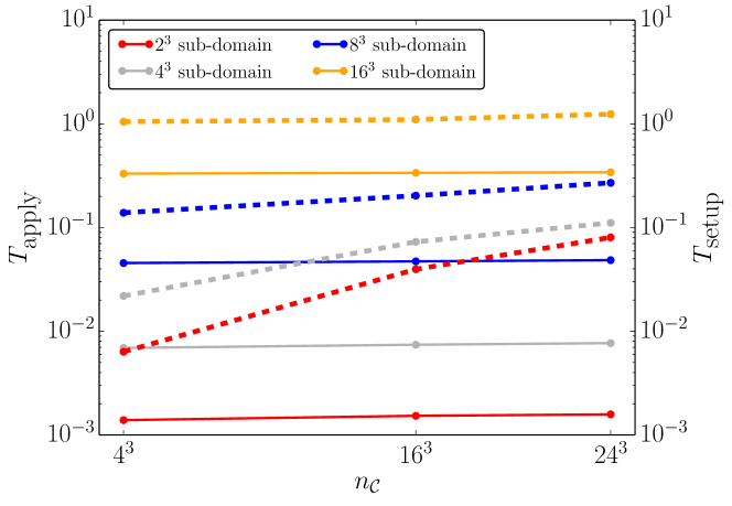
Figure 3: Application time ($T_{\mathrm{apply}}$ – left axis, solid lines) and setup time ($T_{\mathrm{setup}}$ – right axis, dashed lines) as a function of the number of MPI-ranks ($n_{\mathcal{C}}$) for different sub-domain sizes using Disc. B. A constant reduction factor of $r=8$ was used.

From Tables 1 and 2 we observe that for both stencils with low and high numbers of non-zero entries, the setup time required for repartitioning is observed to be only weakly dependent on $r$. In the worst case, reducing the size of the communicator by a factor of 64 is less than two times slower than if the communicator size was reduced by a factor of 8. The time required for application of Telescope (vector permutation and inter-communicator scattering) is more strongly dependent on $r$. For instance, with a coarsening factor of 64, the application takes less than $5$ times longer compared to when $r=8$. In all experiments, the setup time is always larger than the time required to apply the preconditioner. Even when using approximately 32k cores, the setup time is less than 0.2 seconds. From Fig. 3 it is observed that application time of Telescope is independent of the size of the communicator and is only a function of the sub-domain size. For a given sub-domain size, setup times appear to saturate, with small sub-domains ($2^{3}$) saturating at higher core counts compared to experiments using large sub-domains ($16^{3}$).

4.2 Repartitioning at Scale

To demonstrate the performance of Telescope in the context of a multigrid preconditioner, we consider the discrete solution of the 3D elasticity equations (Eq. (3)) for displacement $\boldsymbol{u}$ with $\boldsymbol{g}=\boldsymbol{0}$ in a unit cube domain, $\Omega=[0,1]^{3}$. The constitutive behaviour of the elastic body is assumed to be isotropic, with uniform material properties $E=1$ (Young’s modulus) and $\nu=0.33$ (Poisson ratio) throughout the domain. Deformation is driven by the imposition of the following boundary conditions;

$$\boldsymbol{u}\cdot\boldsymbol{n} =0,\qquad \boldsymbol{t}\cdot\boldsymbol{\sigma}\cdot\boldsymbol{n} =0,\qquad \text{for }z =0,$$

$$\boldsymbol{u}\cdot\boldsymbol{n} =2(\tfrac{1}{2}-x),\qquad \boldsymbol{t}\cdot\boldsymbol{\sigma}\cdot\boldsymbol{n} =0,\qquad \text{for }x =0,1,$$

$$\boldsymbol{u}\cdot\boldsymbol{n} =2(\tfrac{1}{2}-y),\qquad \boldsymbol{t}\cdot\boldsymbol{\sigma}\cdot\boldsymbol{n} =0,\qquad \text{for }y =0,1,$$

$$\boldsymbol{n}\cdot\boldsymbol{\sigma}\cdot\boldsymbol{n} =0,\qquad \boldsymbol{t}\cdot\boldsymbol{\sigma}\cdot\boldsymbol{n} =0,\qquad \text{for }z =1,$$

where $\boldsymbol{n},\boldsymbol{t}$ are the unit vectors normal and tangential to the boundary and $\boldsymbol{\sigma}=\bar{\boldsymbol{C}}\epsilon[\boldsymbol{u}]$ is the Cauchy stress.

The domain $\Omega$ is discretized using $M^{3}$ $Q_{2}$ finite elements defined using the DMDA structured grid object which will be partitioned over the MPI communicator $\mathcal{C}$. Our finite-element implementation has the restriction that each sub-domain assigned to a given MPI-rank must contain at least one $Q_{2}$ element. This implementation restriction defines the depth of a geometric multigrid hierarchy which can be constructed on $\mathcal{C}$, and thus serves as our truncation strategy (see Sec. 1 and 3.3.1).

In these solver experiments, we use FGMRES preconditioned with a single V-cycle of geometric multigrid employing Galerkin coarse-level operators. Iterations are terminated when the initial residual is reduced by a factor of $10^{-8}$. On the coarsest level, we use an inexact Krylov solve (GMRES preconditioned with block-Jacobi) which is terminated when the initial residual is reduced by a factor of $10^{-4}$. On all other levels, we used eight iterations of Richardson’s method, preconditioned with Jacobi as the smoother.

Our experiments consider the end-member scenario associated with strong scaling in which the number of elements per MPI-rank on the finest level is only $2^{3}$. The total number of elements in the mesh is given by $M^{3}$. In Table 3 we report the setup time for Telescope ($T^{tele}_{\text{setup}}$) and solve time ($T_{\text{solve}}$) obtained using either a truncation strategy, or Telescope with different partitioning choices. $T^{tele}_{\text{setup}}$ includes the time required for all phases of the setup, and multiple instances of Telescope. When invoking Telescope in these experiments, the operator was required to be explicitly permuted during the setup phase and thus the time required for $\hat{\mathbf{P}}^{T}\mathbf{A}\hat{\mathbf{P}}$ is included in the value reported for $T^{tele}_{\text{setup}}$. Given the size of the sub-domain considered, truncation variants of multigrid can utilize a hierarchy consisting of only two levels. To obtain raw solve times without hidden setup costs, we report the walltime of the second of two consecutive (identical) solves. All experiments were performed on Edison.

Table 3: Multigrid performance. Shown are the setup time for $\mathtt{Telescope}$ ($T^{tele}_{\mathrm{setup}}$) and solve time ($T_{\mathrm{solve}}$) for different meshes and multigrid configurations. The total number of different resolution meshes is indicated by $N_{L}$. Hierarchical information related to repartitioning (“levels” and “ranks”) are separated by commas, ordered from the finest level (left) to the coarsest level (right).

$M$	levels	$N_{L}$	ranks	$T^{tele}_{\text{setup}}$ (s)	$T_{\text{solve}}$ (s)
32	2	2	$16^{3}$	–	8.34E$-$01
32	2, 3	4	$16^{3}$, $4^{3}$	8.56E$-$02	5.23E$-$01
32	2, 3, 3	6	$16^{3}$, $4^{3}$, 1	9.54E$-$02	1.27E$-$01
64	2	2	$32^{3}$	–	1.48E$+$01
64	2, 3	4	$32^{3}$, $8^{3}$	2.30E$-$01	1.40E$-$01
64	2, 3, 3	6	$32^{3}$, $8^{3}$, $2^{3}$	3.71E$-$01	1.82E$-$01
64	2, 2, 3	5	$32^{3}$, $16^{3}$, $4^{3}$	3.43E$-$01	1.39E$-$01
64	2, 2, 3, 3	7	$32^{3}$, $16^{3}$, $4^{3}$, 1	3.71E$-$01	1.51E$-$01

Table 3 clearly highlights the importance of repartitioning for large-scale problems. Even at 4096 cores, a single stage of repartitioning with $r=64$ yields a time-to-solution which is $1.6\times$ faster than the truncated approach. At the scale of 32k cores, adopting two stages of repartitioning yields a time-to-solution which is approximately $106\times$ faster than the truncated approach. Note that the problem we examined here is “easy” in the sense that there are no spatial variations in the coefficients $E$ or $\nu$. In situations where strong coefficient heterogeneities are present, we expect further improvements in the time-to-solution as the truncated coarse-level solve will become increasingly more difficult to converge. Comparing the results from the two meshes which employed the deepest multigrid hierarchy (e.g. $M=32$: levels = $2,3,3$ cf. $M=64$: levels = $2,2,3,3$), we observe excellent weak scaling behaviour with respect to the solve time. Using 32k cores, introducing two stages of repartitioning causes the setup time to increase by at most a factor of $2.3$ above that required for the configuration using a single stage of repartitioning. The setup cost required by using two (or three) stages of repartitioning (last three rows of Table 3) is larger than the time required for the entire solve on 32k cores. However, we note that the total time for each operation is less than half a second. We also note that the time-to-solution does not always decrease as more stages of repartitioning are used.

4.3 Hybrid CPU-GPU Sub-Domain Smoothers

The trend in emerging and next-generation parallel computing architectures is the inclusion of co-processors (e.g. GPUs or Xeon Phi) on each compute node. Whilst such technology brings a new level of on-node parallelism, it also complicates software development as (i) current discrete high-end GPUs do not share the same memory as the CPU (in the foreseeable future), and (ii) the form of parallelism is sufficiently different from the MPI model for which most large-scale simulation platforms have been designed to support. The development of optimal and scalable algorithms which map to such architectures is essential to enable the next generation of application software to fully exploit the floating point potential offered by hybrid co-processing compute nodes.

In this work we consider casting the multigrid smoother as a restricted additive Schwarz method (RASM) and mapping each sub-domain problem to the accelerator, resulting in a multilevel preconditioner which can utilize many hybrid compute nodes. On each overlapping sub-domain, we perform traditional smoothing such as Chebyshev preconditioned by Jacobi, or Richardson’s method preconditioned by Jacobi. The RASM preconditioner is used with a single Richardson iteration performed on the global problem. The Richardson iteration is performed on the original problem and thus serves as a synchronisation step between the sub-domain problems and the global problem. Experiments with such approaches can be found in [15]. The advantages of this preconditioner are that it avoids latencies in the following two ways: (i) The smoothing operation is local and does not require any inter-node messages to be sent via MPI; (ii) The application of RASM requires only one memory copy from the host to the device (and vice versa) for the input and output vectors, respectively.

Whilst the smoother may be faster to apply than a pure MPI+CPU implementation, it could possess worse smoothing characteristics as a result of the reduced number of synchronization points. However, in the limit of the overlap size equalling the number of smoothing iterations, both methods should be identical. Clearly, a trade-off has to be made between the size of the overlap for each sub-domain, the number of local smoothing iterations to be performed, and the optimal coarsening factor between grid levels.

In Table 4 we present experiments performed on Piz Daint to explore the potential of such hybrid preconditioners when applied to the finite-element discretization of the elasticity operator described in Sec. 3. GPU support within PETSc is facilitated though the ViennaCL library [22] with the OpenCL backend. One design characteristic of the current PETSc-ViennaCL integration is that there is an assumed binding between a single MPI-rank and a GPU. However, to obtain the best per-node performance, we wish to use all cores together with the GPU. This is essential as only the sub-domain smoother is intended to be executed on the GPU. By using Telescope with a reduction factor of $r=8$ and specifying RASM as the preconditioner for the sub-KSP, we can map the sub-domain problem to a single GPU via a single core.

Table 4: Setup and solve times for (i) a CPU only (upper four rows) and (ii) hybrid CPU-GPU RASM multigrid preconditioner. CPU-only experiments are denoted by an “overlap” of “$-$”. Hybrid configurations which are faster than the CPU-only preconditioner are shown in bold.

$M$	levels	overlap	$T_{\text{setup}}$ (s)	Its.	$T_{\text{solve}}$ (s)
8	2	$-$	1.12E$-$02	12	4.27E$-$02
12	3	$-$	4.41E$-$02	16	2.06E$-$01
24	3	$-$	1.88E$-$01	13	1.55E$+$00
48	4	$-$	1.29E$+$00	11	9.92E$+$00
8	2	0	5.49E$-$01	12	2.2813e-01
12	2	0	2.52E$+$00	16	2.3985e-01
24	3	0	4.94E$+$00	13	1.28E$+$00
48	4	0	3.58E$+$01	11	6.66E$+$00
8	2	1	5.95E$-$01	12	2.40E$-$01
12	2	1	1.10E$+$00	16	4.30E$-$01
24	3	1	5.55E$+$00	13	1.52E$+$00
48	4	1	2.30E$+$01	11	7.34E$+$00

All experiments used FGMRES preconditioned with a single V-cycle of geometric multigrid employing re-discretized coarse grid operators. Outer iterations are terminated when the initial residual is reduced by a factor of $10^{-8}$. As a reference, we report computations with a standard CPU-only multigrid preconditioner and compare these results with the RASM - GPU sub-domain smoother (see upper four rows in Table 4). The smoother used in both the CPU-only and the RASM hybrid method consists of Chebyshev(10) preconditioned with Jacobi. The coarse-level solver consisted of one GMRES iteration preconditioned with block-Jacobi (defined over 64 MPI-ranks) and an ILU(0) sub-domain solve. The RASM overlap is defined in terms of the number of $Q_{2}$ elements. Assembled matrices were used on both the CPU and GPU. All experiments were performed on Piz Daint using 8 nodes and all 8 cores per node (64 MPI-ranks in total).

From Table 4 we observe that the iteration counts of the solve are not affected by using a local sub-domain smoother, hence we conclude that the hybrid RASM approach preserves the smoothing properties of the reference smoother (Chebyshev - Jacobi). We also note that cases using an overlap larger than 1 also converged in the same number of iterations as their CPU-only counterpart, however all solve times were larger than using the CPU-only variant. The GPU-based RASM smoother is found to yield improved time-to-solution in several instances.

To understand this behaviour, in Table 5 we report the per-node performance in terms of walltime and FLOP-rate (GF/s) and elements processed per second ($E/s$) achieved by the CPU (using 8 MPI-ranks) and GPU implementations of the sparse matrix vector product (SpMV). We observe that when the mesh contained more than $4^{3}$ elements, the walltime obtained using the GPU SpMV implementation is lower than that obtained using a CPU-only, flat-MPI SpMV. The largest walltime ratio between the GPU and CPU is $\approx 2$. Ignoring all latencies associated with the Aries network, memory addressing and memory copies between the device and host, the best possible improvement in solve time which we can expect for this problem on Piz Daint is thus $\approx 2\times$. For the $M=48$ case with overlap zero, we obtained a solution $\approx 1.5\times$ faster than with the flat-MPI, CPU-only preconditioner.

We emphasize that it is expected that no speed-up was observed when using small sub-domains. For those cases, there is insufficient floating point work for the GPU to perform to offset the overhead associated with kernel launches and the memory copies passing through the PCI Express.

Table 5: Per-node performance of SpMV on Piz Daint. Results were obtained from profiling 100 sparse matrix-vector products for the 3D elasticity operator defined over $M^{3}$ $Q_{2}$ finite elements.

	CPU (8 MPI-ranks)		GPU
$M$	Time (s)	GF/s	$E/s$	Time (s)	GF/s	$E/s$
4	8.89E$-$03	11.99	720k	2.43E$-$02	4.40	264k
8	1.27E$-$01	6.96	402k	5.90E$-$02	14.99	865k
12	4.15E$-$01	7.3	417k	1.91E$-$01	15.91	908k
24	3.15E$+$00	7.79	439k	1.44E$+$00	17.09	963k

5 Discussion

The agglomeration implementation used in Telescope adopts a top-down approach by providing support to coarsen an MPI communicator. In considering the development of general purpose agglomeration algorithms to use within solvers, this choice is most natural. The consequence is that Telescope is most useful in the context of mesh coarsening with a multilevel hierarchy. This is justified assuming the user defines a fine mesh with sub-domains which are well-balanced with respect to computational work and communication requirements. We acknowledge that our approach may lead to a small load imbalance on coarser levels. However, given the reduced volume of work to be performed on these levels, this can be tolerated.

The philosophy used in Telescope differs from the typical approach adopted with unstructured meshes (e.g. UG4 [19]), in which the multigrid hierarchy is created from mesh refinement, and thus the hierarchy of MPI communicators is constructed from refining the size of the communicator assigned to the coarsest level (e.g. MPI-ranks are added). Such a strategy for constructing a hierarchy of MPI communicators is not general enough to support the two use cases discussed in Sec. 3.3.4 and 3.3.5. However, the latter scenario is highly specific to structured grids.

There are a number of memory optimizations which could be applied to the Telescope implementation. Specifically, during the setup phase of the preconditioner, at least one temporary matrix has to be held in memory on the communicator $\mathcal{C}$. In the event that the matrix is to be explicitly permuted, an additional temporary matrix must also be stored. Future work should focus on removing the number of temporary matrices required during the setup phase. Nevertheless, given that the typical use case of Telescope is the redistribution of matrices in which there are very few unknowns per MPI-rank, this storage overhead is not critical.

Currently Telescope only supports repartitioning DMDAs. An obvious extension is to provide support for a wider range of DM implementations, particularly DMPlex, which is the most general mesh representation object provided by PETSc. Extending support to DMPlex likely mandates introducing a new DM interface to permit “refining” the MPI communicator. Such an interface would be of the form DMRefinePartition(DM dm,MPI_Comm rcomm,IS *perm,DM *rdm), where dm is the original mesh, rcomm is the refined MPI communicator, rdm is the repartitioned DM object and perm is an index-set defining the permutation between the original and repartitioned DOF ordering.

Lastly, in the context of the multilevel preconditioners discussed in this work, there is currently no performance model to guide the optimal selection of when agglomeration should occur, and or what the rank reduction factor should be. Future work should automate these choices based on machine characteristics (e.g. network latency, memory access costs), together with characteristics of the matrix (e.g. number of non-zeros per row). An agglomeration performance model is required to support this development.

6 Summary

We have presented an implementation of process agglomeration (or MPI communicator coarsening) called Telescope which has been introduced into the PETSc library. Whilst the development of Telescope was motivated by the need to have a scalable coarse-level solver in the context of a multigrid preconditioner, the design of this agglomeration component is sufficiently general to allow it to be used in many other contexts. Through a series of numerical experiments related to (i) the end-member of a strong scaling study and (ii) a hybrid smoother which utilizes both CPUs and GPUs, we have demonstrated the benefits of this agglomeration implementation.

7 Acknowledgments

The Swiss National Supercomputing Centre (CSCS) and NERSC are thanked for compute time on Piz Daint and Edison respectively. PS acknowledges financial support from the Swiss University Conference and the Swiss Council of Federal Institutes of Technology through the Platform for Advanced Scientific Computing (PASC) program. Some of the authors were supported by the U.S. Department of Energy, Office of Science, Advanced Scientific Computing Research under Contract DE-AC02-06CH11357.

Government License. The submitted manuscript has been created by UChicago Argonne, LLC, Operator of Argonne National Laboratory (“Argonne”). Argonne, a U.S. Department of Energy Office of Science laboratory, is operated under Contract No. DE-AC02-06CH11357. The U.S. Government retains for itself, and others acting on its behalf, a paid-up nonexclusive, irrevocable worldwide license in said article to reproduce, prepare derivative works, distribute copies to the public, and perform publicly and display publicly, by or on behalf of the Government.

References

- [1] M. F. Adams, H. H. Bayraktar, T. M. Keaveny, and P. Papadopoulos. Ultrascalable implicit finite element analyses in solid mechanics with over a half a billion degrees of freedom. In Proceedings of the 2004 ACM/IEEE Conference on Supercomputing, SC ’04, pages 34–, Washington, DC, USA, 2004. IEEE Computer Society.
- [2] S. Balay, S. Abhyankar, M. F. Adams, J. Brown, P. Brune, K. Buschelman, L. Dalcin, V. Eijkhout, W. D. Gropp, D. Kaushik, M. G. Knepley, L. C. McInnes, K. Rupp, B. F. Smith, S. Zampini, and H. Zhang. PETSc users manual. Technical Report ANL-95/11 - Revision 3.6, Argonne National Laboratory, 2015.
- [3] S. Balay, S. Abhyankar, M. F. Adams, J. Brown, P. Brune, K. Buschelman, L. Dalcin, V. Eijkhout, W. D. Gropp, D. Kaushik, M. G. Knepley, L. C. McInnes, K. Rupp, B. F. Smith, S. Zampini, and H. Zhang. PETSc Web page. http://www.mcs.anl.gov/petsc, 2015.
- [4] S. Balay, W. D. Gropp, L. C. McInnes, and B. F. Smith. Efficient management of parallelism in object oriented numerical software libraries. In E. Arge, A. M. Bruaset, and H. P. Langtangen, editors, Modern Software Tools in Scientific Computing, pages 163–202. Birkhäuser Press, 1997.
- [5] M. Blatt, O. Ippisch, and P. Bastian. A massively parallel algebraic multigrid preconditioner based on aggregation for elliptic problems with heterogeneous coefficients. arXiv preprint arXiv:1209.0960v2, 2012.
- [6] J. Brown, B. Smith, and A. Ahmadia. Achieving textbook multigrid efficiency for hydrostatic ice sheet flow. SIAM Journal on Scientific Computing, 35(2):B359–B375, 2013.
- [7] M. Emans. Coarse-grid treatment in parallel AMG for coupled systems in CFD applications. Journal of Computational Science, 2(4):365–376, 2011.
- [8] B. Gmeiner, H. Köstler, M. Stürmer, and U. Rüde. Parallel multigrid on hierarchical hybrid grids: a performance study on current high performance computing clusters. Concurrency and Computation: Practice and Experience, 26(1):217–240, 2014.
- [9] B. Gmeiner, U. Rüde, H. Stengel, C. Waluga, and B. Wohlmuth. Performance and scalability of hierarchical hybrid multigrid solvers for Stokes systems. SIAM Journal on Scientific Computing, 37(2):C143–C168, 2015.
- [10] B. Gmeiner, U. Rüde, H. Stengel, C. Waluga, and B. Wohlmuth. Towards textbook efficiency for parallel multigrid. Numerical Mathematics: Theory, Methods and Applications, 8(01):22–46, 2015.
- [11] T. Hoefler, J. Dinan, D. Buntinas, P. Balaji, B. Barrett, R. Brightwell, W. Gropp, V. Kale, and R. Thakur. MPI + MPI: a new hybrid approach to parallel programming with MPI plus shared memory. Computing, 95(12):1121–1136, 2013.
- [12] T. Isaac, G. Stadler, and O. Ghattas. Solution of nonlinear Stokes equations discretized by high-order finite elements on nonconforming and anisotropic meshes, with application to ice sheet dynamics. SIAM Journal on Scientific Computing, 37(6):B804–B833, 2015.
- [13] S. M. Lechmann, D. A. May, B. J. P. Kaus, and S. M. Schmalholz. Comparing thin-sheet models with 3-D multilayer models for continental collision. Geophysical Journal International, 187(1):10–33, 2011.
- [14] J. Li and O. B. Widlund. On the use of inexact subdomain solvers for BDDC algorithms. Computer Methods in Applied Mechanics and Engineering, 196(8):1415–1428, 2007.
- [15] L. Luo, C. Yang, Y. Zhao, and X.-C. Cai. A scalable hybrid algorithm based on domain decomposition and algebraic multigrid for solving partial differential equations on a cluster of CPU/GPUs. In 2nd International Workshop on GPUs and Scientific Applications (GPUScA 2011), page 45, 2011.
- [16] D. A. May, J. Brown, and L. Le Pourhiet. A scalable, matrix-free multigrid preconditioner for finite element discretizations of heterogeneous Stokes flow. Computer Methods in Applied Mechanics and Engineering, 290:496–523, 2015.
- [17] L. C. McInnes, B. Smith, H. Zhang, and R. T. Mills. Hierarchical Krylov and nested Krylov methods for extreme-scale computing. Parallel Computing, 40(1):17–31, 2014.
- [18] E. H. Müller and R. Scheichl. Massively parallel solvers for elliptic partial differential equations in numerical weather and climate prediction. Quarterly Journal of the Royal Meteorological Society, 140(685):2608–2624, 2014.
- [19] S. Reiter, A. Vogel, I. Heppner, M. Rupp, and G. Wittum. A massively parallel geometric multigrid solver on hierarchically distributed grids. Computing and Visualization in Science, 16(4):151–164, 2013.
- [20] G. Rokos and G. Gorman. PRAgMaTIc–parallel anisotropic adaptive mesh toolkit. In R. Keller, D. Kramer, and J.-P. Weiss, editors, Facing the Multicore-Challenge III, volume 7686 of Lecture Notes in Computer Science, pages 143–144. Springer Berlin Heidelberg, 2013.
- [21] J. Rudi, A. C. I. Malossi, T. Isaac, G. Stadler, M. Gurnis, P. W. Staar, Y. Ineichen, C. Bekas, A. Curioni, and O. Ghattas. An extreme-scale implicit solver for complex PDEs: highly heterogeneous flow in Earth’s mantle. In Proceedings of the International Conference for High Performance Computing, Networking, Storage and Analysis, page 5. ACM, 2015.
- [22] K. Rupp, F. Rudolf, and J. Weinbub. ViennaCL - A high level linear algebra library for GPUs and multi-core CPUs. In International Workshop on GPUs and Scientific Applications, pages 51–56, 2010.
- [23] J. Shewchuk. Triangle: A two-dimensional quality mesh generator and Delaunay triangulator. http://www-2.cs.cmu.edu/~quake/triangle.html, 2005.
- [24] J. R. Shewchuk. Triangle: Engineering a 2D quality mesh generator and Delaunay triangulator. In M. C. Lin and D. Manocha, editors, Applied Computational Geometry: Towards Geometric Engineering, volume 1148 of Lecture Notes in Computer Science, pages 203–222. Springer-Verlag, May 1996. From the 1 ACM Workshop on Applied Computational Geometry.
- [25] H. Si. TetGen: A quality tetrahedral mesh generator and three-dimensional Delaunay triangulator. http://tetgen.berlios.de, 2005.
- [26] H. Si. TetGen, a Delaunay-based quality tetrahedral mesh generator. ACM Transactions on Mathematical Software (TOMS), 41(2), February 2015.
- [27] H. Sundar, G. Biros, C. Burstedde, J. Rudi, O. Ghattas, and G. Stadler. Parallel geometric-algebraic multigrid on unstructured forests of octrees. In Proceedings of the International Conference on High Performance Computing, Networking, Storage and Analysis, page 43. IEEE Computer Society Press, 2012.
- [28] U. Trottenberg, C. W. Oosterlee, and A. Schuller. Multigrid. Academic Press, 2000.