Closed-form Approximations for Coverage and Rate in a Multi-tier Heterogeneous Network in Nakagami-m Fading
G. V. S. S. Praneeth Varma, G. V. V. Sharma, Member, IEEE , and A. Kumar, Member, IEEE
G. V. S. S. Praneeth Varma, G. V. V. Sharma,
and A. Kumar are with the Department of Electrical
Engineering, Indian Institute of Technology Hyderabad,
Kandi, Sangareddy, Telangana 502285, India
(e-mail: {ee14resch11007, gadepall, abhinavkumar}@iith.ac.in ).
Abstract
In this paper, we consider the downlink in a K-tier heterogeneous network in the presence of Nakagami-m fading and noise. For such a system,
we derive closed-form approximations
of coverage probability and average rate achievable.
A piece-wise linear approximation is employed in obtaining the simplified expressions. The proposed results are verified numerically through simulations. A comparison with existing work shows that the proposed work is a good approximation.
Index Terms:
Average rate achievable, coverage probability, Nakagami fading,
path-loss, piece-wise linear approximation.
I Introduction
The demand for higher data rates in cellular networks
has lead to the deployment of small cells along with
the macro base stations (BS) resulting
in multi-tier heterogeneous networks (HetNets).
The irregular BS deployment in such HetNets
can be suitably modeled as a
Poisson point process (PPP) as shown in
[1 ] .
In presence of Rayleigh fading,
a stochastic geometry based
approach has been used to determine
coverage probability and average rate achievable
for multi-tier HetNets in [1 ] .
In the absence of simple analytical
expressions of coverage and rate,
ordering results for various transmission techniques
in multi-antenna HetNets with Rayleigh fading
for an interference limited scenario
have been presented in [2 ] .
In [3 ] , average rate for generalized fading channels were derived using an MGF approach. An expression for the coverage
probability was derived in semi-closed form for the dual branch in multi-antenna single tier network in [4 ] . Coverage and rate were derived using the gil-peleaz inversion formula in [5 ] . Analytical results in the above literature were expressed in either single or two fold integrals. A closed form expression for outage in the presence of rayleigh fading for a single tier network in terms of a toeplitz matrix was obtained in [6 ] . This problem was extended and solved for MIMO in [7 ] , where the decision variable involved Gamma random variables. However, both the above papers focused on interference limited systems.
Thus, simplified analytical expressions
for coverage and rate in the presence of
Nakagami-m fading for both noise and interference
limited scenarios are required. This is the motivation of this work. The coverage expressions obtained in our work are approximate, but the approach is extremely simple and the results quite accurate.
The system model considered in this paper is presented next.
II System model
We consider a K 𝐾 K i 𝑖 i Φ i subscript Φ 𝑖 \Phi_{i} λ i subscript 𝜆 𝑖 \lambda_{i} i 𝑖 i P i subscript 𝑃 𝑖 P_{i} β i subscript 𝛽 𝑖 \beta_{i} x i subscript 𝑥 𝑖 x_{i} L ( x i ) = ‖ x i ‖ − α 𝐿 subscript 𝑥 𝑖 superscript norm subscript 𝑥 𝑖 𝛼 L(x_{i})=||x_{i}||^{-\alpha} x i subscript 𝑥 𝑖 x_{i} i 𝑖 i
S I N R ( x i ) = P i h x i ‖ x i ‖ − α ∑ j = 1 K ∑ x ∈ Φ j \ x i P j h x ‖ x ‖ − α + σ 2 , 𝑆 𝐼 𝑁 𝑅 subscript 𝑥 𝑖 subscript 𝑃 𝑖 subscript ℎ subscript 𝑥 𝑖 superscript norm subscript 𝑥 𝑖 𝛼 superscript subscript 𝑗 1 𝐾 subscript 𝑥 \ subscript Φ 𝑗 subscript 𝑥 𝑖 subscript 𝑃 𝑗 subscript ℎ 𝑥 superscript norm 𝑥 𝛼 superscript 𝜎 2 SINR(x_{i})=\frac{P_{i}h_{x_{i}}||x_{i}||^{-\alpha}}{\sum_{j=1}^{K}\sum_{x\in\Phi_{j}\backslash x_{i}}P_{j}h_{x}||x||^{-\alpha}+\sigma^{2}}\,, (1)
where,
h x i subscript ℎ subscript 𝑥 𝑖 h_{x_{i}} x i subscript 𝑥 𝑖 {x_{i}} σ 2 superscript 𝜎 2 \sigma^{2} h x i ∼ Γ ( M i , 1 ) similar-to subscript ℎ subscript 𝑥 𝑖 Γ subscript 𝑀 𝑖 1 h_{x_{i}}\sim\Gamma(M_{i},1) i 𝑖 i h x i subscript ℎ subscript 𝑥 𝑖 h_{x_{i}} 𝐂 ( { β i } ) 𝐂 subscript 𝛽 𝑖 \mathbf{C}(\{\beta_{i}\}) { β i } subscript 𝛽 𝑖 \{\beta_{i}\}
𝐂 ( { β i } ) ≜ ∪ i ∈ K , x i ∈ Φ i ( S I N R ( x i ) > β i ) . ≜ 𝐂 subscript 𝛽 𝑖 subscript formulae-sequence 𝑖 𝐾 subscript 𝑥 𝑖 subscript Φ 𝑖 𝑆 𝐼 𝑁 𝑅 subscript 𝑥 𝑖 subscript 𝛽 𝑖 \mathbf{C}(\{\beta_{i}\})\triangleq\cup_{i\in K,x_{i}\in\Phi_{i}}(SINR(x_{i})>\beta_{i})\,. (2)
Then, from [1 ] ,
the coverage probability P c subscript 𝑃 𝑐 P_{c} m 𝑚 m
P c = ℙ ( 𝐂 ( { β i } ) ) = ℙ ( ∪ i ∈ K , x i ∈ Φ i ( S I N R ( x i ) > β i ) ) . subscript 𝑃 𝑐 ℙ 𝐂 subscript 𝛽 𝑖 ℙ subscript formulae-sequence 𝑖 𝐾 subscript 𝑥 𝑖 subscript Φ 𝑖 𝑆 𝐼 𝑁 𝑅 subscript 𝑥 𝑖 subscript 𝛽 𝑖 P_{c}=\mathbb{P}\left(\mathbf{C}(\{\beta_{i}\})\right)=\mathbb{P}\left(\ \cup_{i\in K,x_{i}\in\Phi_{i}}(SINR(x_{i})>\beta_{i})\right)\,. (3)
Under the assumption β i > 1 subscript 𝛽 𝑖 1 \beta_{i}>1 1 3 [1 ]
P c = ∑ i = 1 K λ i ∫ R 2 ℙ ( P i h x i L ( x i ) I x i + σ 2 > β i ) 𝑑 x i . subscript 𝑃 𝑐 superscript subscript 𝑖 1 𝐾 subscript 𝜆 𝑖 subscript superscript 𝑅 2 ℙ subscript 𝑃 𝑖 subscript ℎ subscript 𝑥 𝑖 𝐿 subscript 𝑥 𝑖 subscript 𝐼 subscript 𝑥 𝑖 superscript 𝜎 2 subscript 𝛽 𝑖 differential-d subscript 𝑥 𝑖 P_{c}=\sum_{i=1}^{K}\lambda_{i}\int_{R^{2}}\mathbb{P}\left(\frac{P_{i}h_{x_{i}}L(x_{i})}{I_{x_{i}}+\sigma^{2}}>\beta_{i}\right)dx_{i}\,. (4)
ℐ i subscript ℐ 𝑖 \displaystyle\mathcal{I}_{i} = \displaystyle= ∑ k = 0 M i − 1 1 k ! ∑ l = 0 k ( k l ) ( σ 2 ) k − l ( − 1 ) l A α 2 ( k − l ) + 1 ∑ r = 0 l ( − 1 ) r B l , r ( D 1 , D 2 , … , D l − r + 1 ) [ c { γ ( r + α 2 ( k − l ) + 1 , A ( σ 2 ) 2 / α x 2 ) − γ ( r + α 2 ( k − l ) + 1 , A ( σ 2 ) 2 / α x 1 ) } \displaystyle\sum_{k=0}^{M_{i}-1}\frac{1}{k!}\sum_{l=0}^{k}\binom{k}{l}\frac{(\sigma^{2})^{k-l}(-1)^{l}}{A^{\frac{\alpha}{2}(k-l)+1}}\sum_{r=0}^{l}(-1)^{r}B_{l,r}(D_{1},D_{2},\dots,D_{l-r+1}){}\left[c\left\{\gamma\left(r+\frac{\alpha}{2}(k-l)+1,\frac{A}{(\sigma^{2})^{2/\alpha}}x_{2}\right)\right.\left.-\gamma\left(r+\frac{\alpha}{2}(k-l)+1,\frac{A}{(\sigma^{2})^{2/\alpha}}x_{1}\right)\right\}\right. (9)
+ γ ( r + α 2 ( k − l ) + 1 , A ( σ 2 ) 2 / α x 1 ) + ( σ 2 ) 2 / α A m { γ ( r + α 2 ( k − l ) + 2 , A ( σ 2 ) 2 / α x 2 ) − γ ( r + α 2 ( k − l ) + 2 , A ( σ 2 ) 2 / α x 1 ) } ] \displaystyle+\gamma\left(r+\frac{\alpha}{2}(k-l)+1,\frac{A}{(\sigma^{2})^{2/\alpha}}x_{1}\right)+\frac{(\sigma^{2})^{2/\alpha}}{A}m\left\{\gamma\left(r+\frac{\alpha}{2}(k-l)+2,\frac{A}{(\sigma^{2})^{2/\alpha}}x_{2}\right)\right.{}\left.\left.-\gamma\left(r+\frac{\alpha}{2}(k-l)+2,\frac{A}{(\sigma^{2})^{2/\alpha}}x_{1}\right)\right\}\right]
Given that the user is in coverage,
the average rate achievable
for Nakagami-m fading is expressed in [1 ] as
R = 𝔼 [ l o g ( 1 + m a x x ∈ ∪ Φ i ( S I N R ( x ) ) | 𝐂 ( { β i } ) ) ] , 𝑅 𝔼 delimited-[] 𝑙 𝑜 𝑔 1 conditional 𝑥 subscript Φ 𝑖 𝑚 𝑎 𝑥 𝑆 𝐼 𝑁 𝑅 𝑥 𝐂 subscript 𝛽 𝑖 R=\mathbb{E}\left[log\left(1+\left.\underset{x\in\cup\Phi_{i}}{max}\,(SINR(x))\right|\mathbf{C}(\{\beta_{i}\})\right)\right]\,,
which simplifies to
R = ∫ 0 ∞ ℙ ( X > y | 𝐂 ( { β i } ) ) 1 + y 𝑑 y , 𝑅 superscript subscript 0 ℙ 𝑋 conditional 𝑦 𝐂 subscript 𝛽 𝑖 1 𝑦 differential-d 𝑦 R=\int_{0}^{\infty}\frac{\mathbb{P}(X>y|\mathbf{C}(\{\beta_{i}\}))}{1+y}dy\,, (5)
where,
ℙ ( X > y | 𝐂 ( { β i } ) ) = ℙ ( 𝐂 ( { m a x ( y , β i ) } ) ) ℙ ( 𝐂 ( { β i } ) ) . ℙ 𝑋 conditional 𝑦 𝐂 subscript 𝛽 𝑖 ℙ 𝐂 𝑚 𝑎 𝑥 𝑦 subscript 𝛽 𝑖 ℙ 𝐂 subscript 𝛽 𝑖 \mathbb{P}(X>y|\mathbf{C}(\{\beta_{i}\}))=\frac{\mathbb{P}(\mathbf{C}(\{max(y,\beta_{i})\}))}{\mathbb{P}(\mathbf{C}(\{\beta_{i}\}))}. (6)
Next, we present the main results of this paper.
III Coverage Probability
A commonly encountered integral
in the coverage analysis
using stochastic geometry based approach, as in [1 ] [2 ] , is
∫ 0 ∞ e − V t − U t α 2 t n 2 𝑑 t . superscript subscript 0 superscript 𝑒 𝑉 𝑡 𝑈 superscript 𝑡 𝛼 2 superscript 𝑡 𝑛 2 differential-d 𝑡 \int_{0}^{\infty}e^{-Vt-Ut^{\frac{\alpha}{2}}}t^{\frac{n}{2}}\,dt\,. (7)
For approximating (7
Theorem III.1 .
For α > 2 𝛼 2 \alpha>2 U > 0 𝑈 0 U>0 V > 0 𝑉 0 V>0
∫ 0 ∞ e − V t − U t α 2 t n 2 d t ≈ 1 V n + 2 2 [ γ ( n / 2 + 1 , V U 2 / α x 1 ) + c { γ ( n / 2 + 1 , V U 2 / α x 2 ) − γ ( n / 2 + 1 , V U 2 / α x 1 ) } + U 2 / α V m { γ ( n / 2 + 2 , V U 2 / α x 2 ) − γ ( n / 2 + 2 , V U 2 / α x 1 ) } ] , superscript subscript 0 superscript 𝑒 𝑉 𝑡 𝑈 superscript 𝑡 𝛼 2 superscript 𝑡 𝑛 2 𝑑 𝑡 1 superscript 𝑉 𝑛 2 2 delimited-[] 𝛾 𝑛 2 1 𝑉 superscript 𝑈 2 𝛼 subscript 𝑥 1 𝑐 𝛾 𝑛 2 1 𝑉 superscript 𝑈 2 𝛼 subscript 𝑥 2 𝛾 𝑛 2 1 𝑉 superscript 𝑈 2 𝛼 subscript 𝑥 1 superscript 𝑈 2 𝛼 𝑉 𝑚 𝛾 𝑛 2 2 𝑉 superscript 𝑈 2 𝛼 subscript 𝑥 2 𝛾 𝑛 2 2 𝑉 superscript 𝑈 2 𝛼 subscript 𝑥 1 \int_{0}^{\infty}e^{-Vt-Ut^{\frac{\alpha}{2}}}t^{\frac{n}{2}}\,dt\approx\frac{1}{V^{\frac{n+2}{2}}}{}\left[\gamma\left(n/2+1,\frac{V}{U^{2/\alpha}}x_{1}\right)\right.\\
+c\left\{\gamma\left(n/2+1,\frac{V}{U^{2/\alpha}}x_{2}\right)-\gamma\left(n/2+1,\frac{V}{U^{2/\alpha}}x_{1}\right)\right\}\\
+{}\left.\frac{U^{2/\alpha}}{V}m\left\{\gamma\left(n/2+2,\frac{V}{U^{2/\alpha}}x_{2}\right)-\gamma\left(n/2+2,\frac{V}{U^{2/\alpha}}x_{1}\right)\right\}\right]\,, (8)
where, m = − α 2 ( 1 − 2 α ) 1 − 2 α e − ( 1 − 2 α ) 𝑚 𝛼 2 superscript 1 2 𝛼 1 2 𝛼 superscript 𝑒 1 2 𝛼 m=-\frac{\alpha}{2}\left(1-\frac{2}{\alpha}\right)^{1-\frac{2}{\alpha}}e^{-\left(1-\frac{2}{\alpha}\right)} c = α 2 e − ( 1 − 2 α ) 𝑐 𝛼 2 superscript 𝑒 1 2 𝛼 c=\frac{\alpha}{2}e^{-(1-\frac{2}{\alpha})} x 1 = 1 − c m subscript 𝑥 1 1 𝑐 𝑚 x_{1}=\frac{1-c}{m} x 2 = − c m subscript 𝑥 2 𝑐 𝑚 x_{2}=\frac{-c}{m} γ ( ⋅ , ⋅ ) 𝛾 ⋅ ⋅ \gamma\left(\cdot,\cdot\right) [8 , 8.350] .
Next, we present our main result for the
coverage probability in a K-tier HetNet.
Theorem III.2 .
The coverage probability of K-tier HetNet in Nakagami fading, when β i > 1 subscript 𝛽 𝑖 1 \beta_{i}>1
P c = ∑ i = 1 K π λ i P i 2 / α β i − 2 / α ℐ i , subscript 𝑃 𝑐 superscript subscript 𝑖 1 𝐾 𝜋 subscript 𝜆 𝑖 superscript subscript 𝑃 𝑖 2 𝛼 superscript subscript 𝛽 𝑖 2 𝛼 subscript ℐ 𝑖 P_{c}=\sum_{i=1}^{K}\pi\lambda_{i}P_{i}^{2/\alpha}\beta_{i}^{-2/\alpha}\mathcal{I}_{i}\,, (10)
where, ℐ i subscript ℐ 𝑖 \mathcal{I}_{i} 9 D t = ∏ q = 0 t − 1 ( 2 α − q ) subscript 𝐷 𝑡 superscript subscript product 𝑞 0 𝑡 1 2 𝛼 𝑞 D_{t}=\prod_{q=0}^{t-1}\left(\frac{2}{\alpha}-q\right) ( k l ) = k ! l ! ( k − l ) ! binomial 𝑘 𝑙 𝑘 𝑙 𝑘 𝑙 \binom{k}{l}=\frac{k!}{l!(k-l)!} A = ∑ m = 1 K λ m ( P m ) 2 / α ∑ p = 1 M m ( M m p ) 2 π α ℬ ( M m − p + 2 / α , p − 2 / α ) 𝐴 superscript subscript 𝑚 1 𝐾 subscript 𝜆 𝑚 superscript subscript 𝑃 𝑚 2 𝛼 superscript subscript 𝑝 1 subscript 𝑀 𝑚 binomial subscript 𝑀 𝑚 𝑝 2 𝜋 𝛼 ℬ subscript 𝑀 𝑚 𝑝 2 𝛼 𝑝 2 𝛼 A=\sum_{m=1}^{K}\lambda_{m}(P_{m})^{2/\alpha}\sum_{p=1}^{M_{m}}\binom{M_{m}}{p}\frac{2\pi}{\alpha}\mathcal{B}(M_{m}-p+2/\alpha,p-2/\alpha) ℬ ( ⋅ , ⋅ ) ℬ ⋅ ⋅ \mathcal{B}\left(\cdot,\cdot\right) [8 , 8.380] and the Bell polynomial is defined as
B l , r ( x 1 , x 2 , … , x l − r + 1 ) = ∑ l ! j 1 ! j 2 ! … j l − r + 1 ! ∏ t = 1 l − r + 1 ( x t t ! ) j t subscript 𝐵 𝑙 𝑟
subscript 𝑥 1 subscript 𝑥 2 … subscript 𝑥 𝑙 𝑟 1 𝑙 subscript 𝑗 1 subscript 𝑗 2 … subscript 𝑗 𝑙 𝑟 1 superscript subscript product 𝑡 1 𝑙 𝑟 1 superscript subscript 𝑥 𝑡 𝑡 subscript 𝑗 𝑡 B_{l,r}(x_{1},x_{2},\dots,x_{l-r+1})=\sum\frac{l!}{j_{1}!j_{2}!\dots j_{l-r+1}!}\prod_{t=1}^{l-r+1}\left(\frac{x_{t}}{t!}\right)^{j_{t}} (11)
summation is over all j 𝑗 j j 1 + j 2 + ⋯ + j l − r + 1 = r subscript 𝑗 1 subscript 𝑗 2 ⋯ subscript 𝑗 𝑙 𝑟 1 𝑟 j_{1}+j_{2}+\dots+j_{l-r+1}=r j 1 + 2 j 2 + ⋯ + ( l − r + 1 ) j l − r + 1 = l subscript 𝑗 1 2 subscript 𝑗 2 ⋯ 𝑙 𝑟 1 subscript 𝑗 𝑙 𝑟 1 𝑙 j_{1}+2j_{2}+\dots+(l-r+1)j_{l-r+1}=l
Corollary III.3 .
In the presence of Rayleigh fading, i.e., M i = 1 subscript 𝑀 𝑖 1 M_{i}=1
P c subscript 𝑃 𝑐 \displaystyle P_{c} = ∑ i = 1 K π λ i P i 2 / α β i − 2 / α V [ ( 1 − e − V U 2 / α x 1 ) + c ( e − V U 2 / α x 1 − e − V U 2 / α x 2 ) \displaystyle=\sum_{i=1}^{K}\frac{\pi\lambda_{i}P_{i}^{2/\alpha}\beta_{i}^{-2/\alpha}}{V}\left[\left(1-e^{-\frac{V}{U^{2/\alpha}}x_{1}}\right)+c\left(e^{-\frac{V}{U^{2/\alpha}}x_{1}}-e^{-\frac{V}{U^{2/\alpha}}x_{2}}\right)\right.
+ m { e − V U 2 / α x 1 ( x 1 + U 2 / α V ) − e − V U 2 / α x 2 ( x 2 + U 2 / α V ) } ] , \displaystyle\quad+m\left\{e^{-\frac{V}{U^{2/\alpha}}x_{1}}\left(x_{1}+\frac{U^{2/\alpha}}{V}\right)\right.\left.\left.-e^{-\frac{V}{U^{2/\alpha}}x_{2}}\left(x_{2}+\frac{U^{2/\alpha}}{V}\right)\right\}\right]\,, (12)
where, V = 2 π α Γ ( 2 / α ) Γ ( 1 − 2 / α ) ∑ m = 1 K λ m P m 2 / α 𝑉 2 𝜋 𝛼 Γ 2 𝛼 Γ 1 2 𝛼 superscript subscript 𝑚 1 𝐾 subscript 𝜆 𝑚 superscript subscript 𝑃 𝑚 2 𝛼 V=\frac{2\pi}{\alpha}\Gamma(2/\alpha)\Gamma(1-2/\alpha)\sum_{m=1}^{K}\lambda_{m}P_{m}^{2/\alpha} and
U = σ 2 𝑈 superscript 𝜎 2 U=\sigma^{2}
Proof.
Substituting M i = 1 subscript 𝑀 𝑖 1 M_{i}=1 10 γ ( 1 + z , x ) = z ! [ 1 − e − x ∑ k = 0 z x k k ! ] , ∀ z ∈ ℤ formulae-sequence 𝛾 1 𝑧 𝑥 𝑧 delimited-[] 1 superscript 𝑒 𝑥 superscript subscript 𝑘 0 𝑧 superscript 𝑥 𝑘 𝑘 for-all 𝑧 ℤ \gamma(1+z,x)=z!\left[1-e^{-x}\sum_{k=0}^{z}\frac{x^{k}}{k!}\right],\forall\,z\in\mathbb{Z} III.3
[1 , (2)] .
Next, we present results for
the average rate achievable of a typical UE.
IV Average Rate
Theorem IV.1 .
The average rate achievable of a typical UE in coverage
of a K-tier HetNet
in Nakagami fading, when β i > 1 subscript 𝛽 𝑖 1 \beta_{i}>1
R = ∑ i = 1 K λ i P i 2 / α β i − 2 / α 𝒜 i ℐ i ∑ i = 1 K λ i P i 2 / α β i − 2 / α ℐ i , 𝑅 superscript subscript 𝑖 1 𝐾 subscript 𝜆 𝑖 superscript subscript 𝑃 𝑖 2 𝛼 superscript subscript 𝛽 𝑖 2 𝛼 subscript 𝒜 𝑖 subscript ℐ 𝑖 superscript subscript 𝑖 1 𝐾 subscript 𝜆 𝑖 superscript subscript 𝑃 𝑖 2 𝛼 superscript subscript 𝛽 𝑖 2 𝛼 subscript ℐ 𝑖 R=\frac{\sum_{i=1}^{K}\lambda_{i}P_{i}^{2/\alpha}\beta_{i}^{-2/\alpha}\mathcal{A}_{i}\mathcal{I}_{i}}{\sum_{i=1}^{K}\lambda_{i}P_{i}^{2/\alpha}\beta_{i}^{-2/\alpha}\mathcal{I}_{i}}\,, (13)
where, ℐ i subscript ℐ 𝑖 \mathcal{I}_{i} 9
𝒜 i subscript 𝒜 𝑖 \displaystyle\mathcal{A}_{i} = ln ( 1 + β i ) + α 2 2 F 1 ( 1 , 2 α , 1 + 2 α ; − 1 β i ) , absent 1 subscript 𝛽 𝑖 subscript 𝛼 2 2 subscript 𝐹 1 1 2 𝛼 1 2 𝛼 1 subscript 𝛽 𝑖 \displaystyle=\ln\left(1+\beta_{i}\right)+\frac{\alpha}{2}\ _{2}F_{1}\left(1,\frac{2}{\alpha},1+\frac{2}{\alpha};-\frac{1}{\beta_{i}}\right)\,, (14)
and F 1 2 ( . ) {}_{2}F_{1}(.) [9 ] .
Proof.
Corollary IV.2 .
In the presence of Rayleigh fading,
i.e., M i = 1 subscript 𝑀 𝑖 1 M_{i}=1
R = ∑ i = 1 K λ i P i 2 / α β i − 2 / α 𝒜 i ∑ i = 1 K λ i P i 2 / α β i − 2 / α . 𝑅 superscript subscript 𝑖 1 𝐾 subscript 𝜆 𝑖 superscript subscript 𝑃 𝑖 2 𝛼 superscript subscript 𝛽 𝑖 2 𝛼 subscript 𝒜 𝑖 superscript subscript 𝑖 1 𝐾 subscript 𝜆 𝑖 superscript subscript 𝑃 𝑖 2 𝛼 superscript subscript 𝛽 𝑖 2 𝛼 R=\frac{\sum_{i=1}^{K}\lambda_{i}P_{i}^{2/\alpha}\beta_{i}^{-2/\alpha}\mathcal{A}_{i}}{\sum_{i=1}^{K}\lambda_{i}P_{i}^{2/\alpha}\beta_{i}^{-2/\alpha}}\,. (15)
Proof.
Substituting M i = 1 subscript 𝑀 𝑖 1 M_{i}=1 9 I i subscript 𝐼 𝑖 I_{i} i 𝑖 i 13 15
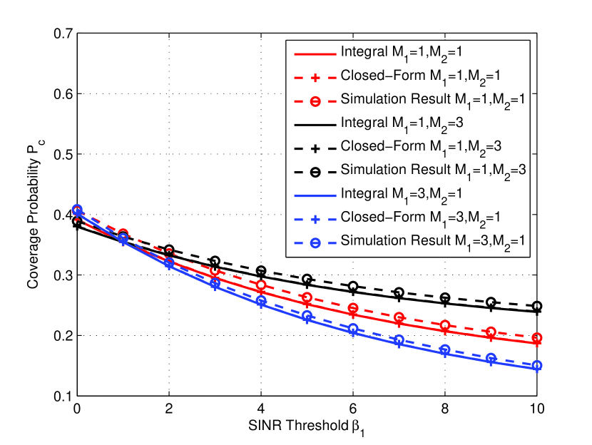
Figure 1: Variation of P c subscript 𝑃 𝑐 P_{c} β 1 subscript 𝛽 1 \beta_{1} ( K = 2 , α = 3 , P 1 = 25 P 2 , λ 2 = 5 λ 1 , β 2 = 1 d B ) formulae-sequence 𝐾 2 formulae-sequence 𝛼 3 formulae-sequence subscript 𝑃 1 25 subscript 𝑃 2 formulae-sequence subscript 𝜆 2 5 subscript 𝜆 1 subscript 𝛽 2 1 𝑑 𝐵 (K=2,\alpha=3,P_{1}=25P_{2},\lambda_{2}=5\lambda_{1},\beta_{2}=1dB)
V Numerical Results
We consider the simulation setup as in [1 ] , a two-tier HetNet consisting of macro BSs
and small cells.
We performed Monte Carlo simulations in MATLAB
to obtain the simulation results which are averaged over 10 4 superscript 10 4 10^{4} 10 3 superscript 10 3 10^{3} [1 ] and the proposed approximate
expressions in MATLAB.
In Fig. 1 P c subscript 𝑃 𝑐 P_{c} β 1 subscript 𝛽 1 \beta_{1}
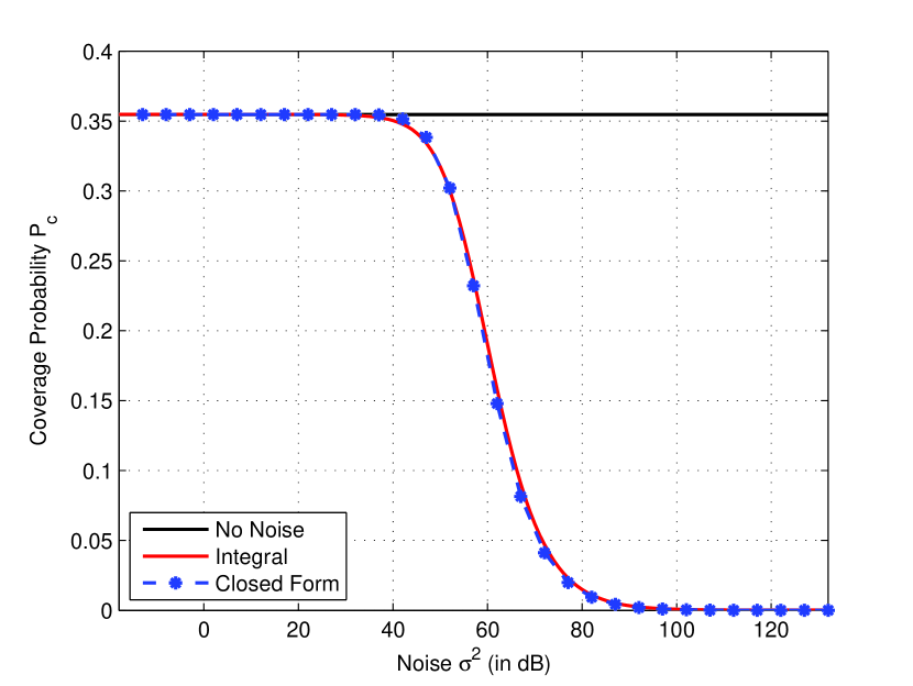
The curve generated using (10 [1 , (2)] and the simulation results for various values of the Nakagami parameters, M 1 subscript 𝑀 1 M_{1} M 2 subscript 𝑀 2 M_{2} P c subscript 𝑃 𝑐 P_{c} σ 2 superscript 𝜎 2 \sigma^{2} 2 σ 2 superscript 𝜎 2 \sigma^{2}
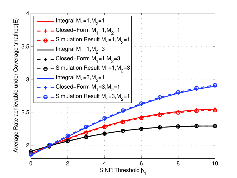
In Fig. 3 R 𝑅 R β 1 subscript 𝛽 1 \beta_{1} 13 [1 , (7)] and
the simulation results as observed in Fig. 3 Through extensive numerical computation
it was verified that
the percentage loss in approximation of
P c subscript 𝑃 𝑐 P_{c} 10 8 0.5 % percent 0.5 0.5\% α 𝛼 \alpha M i subscript 𝑀 𝑖 M_{i} .
Figure 2: Variation of P c subscript 𝑃 𝑐 P_{c} σ 2 superscript 𝜎 2 \sigma^{2} ( K = 2 , α = 3 , P 1 = 25 P 2 , λ 2 = 5 λ 1 , β 1 = 1 d B , β 2 = 1 d B ) formulae-sequence 𝐾 2 formulae-sequence 𝛼 3 formulae-sequence subscript 𝑃 1 25 subscript 𝑃 2 formulae-sequence subscript 𝜆 2 5 subscript 𝜆 1 formulae-sequence subscript 𝛽 1 1 𝑑 𝐵 subscript 𝛽 2 1 𝑑 𝐵 (K=2,\alpha=3,P_{1}=25P_{2},\lambda_{2}=5\lambda_{1},\beta_{1}=1dB,\beta_{2}=1dB) Figure 3: Variation of R 𝑅 R β 1 subscript 𝛽 1 \beta_{1} ( K = 2 , α = 3 , P 1 = 25 P 2 , λ 2 = 5 λ 1 , β 2 = 1 d B ) formulae-sequence 𝐾 2 formulae-sequence 𝛼 3 formulae-sequence subscript 𝑃 1 25 subscript 𝑃 2 formulae-sequence subscript 𝜆 2 5 subscript 𝜆 1 subscript 𝛽 2 1 𝑑 𝐵 (K=2,\alpha=3,P_{1}=25P_{2},\lambda_{2}=5\lambda_{1},\beta_{2}=1dB)
VI Conclusion
We have proposed closed-form approximations
for coverage probability and average rate achievable
in a K-tier HetNet in the presence of noise and Nakagami fading. Further, through simulation results
we have shown that the proposed simplified expressions match closely with existing results.
References
[1]
H. Dhillon, R. Ganti, F. Baccelli, and J. G. Andrews, “Modeling and analysis
of k-tier downlink heterogeneous cellular networks,” IEEE J. Sel.
Areas Commun. , vol. 30, no. 3, pp. 550–560, April 2012.
[2]
H. S. Dhillon, M. Kountouris, and J. G. Andrews, “Downlink mimo hetnets:
Modeling,ordering results and performance analysis,” IEEE Trans.
Wireless Commun. , vol. 12, no. 10, pp. 5208–5222, October 2013.
[3]
M. D. Renzo, A. Guidotti, and G. Corazza, “Average rate of downlink
heterogeneous cellular networks over generalized fading channels: A
stochastic geometry approach,” IEEE Trans. Commun. , vol. 61, no. 7,
pp. 3050–3071, July 2013.
[4]
R. Tanbourgi, H. S. Dhillon, J. G. Andrews, and F. K. Jondral, “Dual-branch
mrc receivers under spatial interference correlation and nakagami fading,”
IEEE Trans. Commun. , vol. 62, no. 6, pp. 1830–1844, June 2014.
[5]
M. D. Renzo and P. Guan, “Stochastic geometry modeling of coverage and rate of
cellular networks using the gil-pelaez inversion theorem,” IEEE
Commun. Lett. , vol. 18, no. 9, pp. 1575–1578, Sept 2014.
[6]
C. Li, J. Zhang, and K. Letaief, “Throughput and energy efficiency analysis of
small cell networks with multi-antenna base stations,” IEEE Trans.
Wireless Commun , vol. 13, no. 5, pp. 2505 – 2517, May 2014.
[7]
C. Li, J. Zhang, J. G. Andrews, and K. Letaief, “Success probability and area
spectral efficiency in multiuser mimo hetnets,” IEEE Trans. Commun. ,
vol. 64, no. 4, pp. 1544 – 1556, April 2016.
[8]
S. Gradshteyn and I. Ryzhik, Table of Integrals, Series, and Products ,
7th ed. Academic Press, 2007.
[9]
M. E. Hazewinkel, Encyclopaedia of Mathematics . Kluwer Academic Publishers, 1994.
Appendix A Proof of Theorem III.1
The expression in (8
∫ 0 ∞ e − U t α / 2 e − V t t n 2 𝑑 t = 1 U n + 2 α ∫ 0 ∞ e − y α 2 e − V U 2 / α y y n / 2 𝑑 y . superscript subscript 0 superscript 𝑒 𝑈 superscript 𝑡 𝛼 2 superscript 𝑒 𝑉 𝑡 superscript 𝑡 𝑛 2 differential-d 𝑡 1 superscript 𝑈 𝑛 2 𝛼 superscript subscript 0 superscript 𝑒 superscript 𝑦 𝛼 2 superscript 𝑒 𝑉 superscript 𝑈 2 𝛼 𝑦 superscript 𝑦 𝑛 2 differential-d 𝑦 \int_{0}^{\infty}e^{-Ut^{\alpha/2}}e^{-Vt}t^{\frac{n}{2}}dt=\frac{1}{U^{\frac{n+2}{\alpha}}}\int_{0}^{\infty}e^{-y^{\frac{\alpha}{2}}}e^{-\frac{V}{U^{2/\alpha}}y}y^{n/2}dy\,. (16)
It is difficult to obtain an exact
closed form solution for
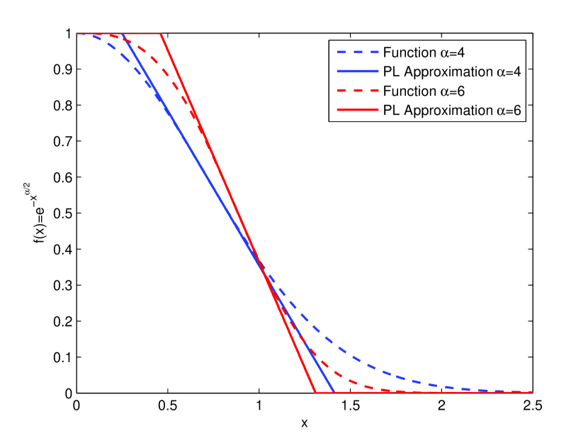
(16 α 𝛼 \alpha 4 f ( x ) = e − x α / 2 𝑓 𝑥 superscript 𝑒 superscript 𝑥 𝛼 2 f(x)=e^{-x^{\alpha/2}} x 𝑥 x f ( x ) ∈ ( 0 , 1 ] ∀ x ≥ 0 𝑓 𝑥 0 1 for-all 𝑥 0 f(x)\in(0,1]\,\forall x\geq 0 f ( x ) = e − x α / 2 𝑓 𝑥 superscript 𝑒 superscript 𝑥 𝛼 2 f(x)=e^{-x^{\alpha/2}}
e − x α / 2 ≈ { 1 x ≤ x 1 , m x + c x 1 < x < x 2 , 0 x 2 ≤ x , superscript 𝑒 superscript 𝑥 𝛼 2 cases 1 𝑥 subscript 𝑥 1 𝑚 𝑥 𝑐 subscript 𝑥 1 𝑥 subscript 𝑥 2 0 subscript 𝑥 2 𝑥 e^{-x^{\alpha/2}}\approx\left\{\begin{array}[]{ll}1&x\leq x_{1}\,,\\
mx+c&x_{1}<x<x_{2}\,,\\
0&x_{2}\leq x\,,\end{array}\right. (17)
where, m 𝑚 m x 1 subscript 𝑥 1 x_{1} x 2 subscript 𝑥 2 x_{2} c 𝑐 c
Figure 4: Piecewise linear approximation
To obtain m 𝑚 m f ( x ) 𝑓 𝑥 f(x) x 0 subscript 𝑥 0 x_{0}
d 2 ( e − x α / 2 ) d x 2 | x = x 0 = 0 ⇒ x 0 = ( 1 − 2 α ) 2 α . evaluated-at superscript 𝑑 2 superscript 𝑒 superscript 𝑥 𝛼 2 𝑑 superscript 𝑥 2 𝑥 subscript 𝑥 0 0 ⇒ subscript 𝑥 0 superscript 1 2 𝛼 2 𝛼 \left.\frac{d^{2}(e^{-x^{\alpha/2}})}{dx^{2}}\right|_{x=x_{0}}=0\Rightarrow x_{0}=\left(1-\frac{2}{\alpha}\right)^{\frac{2}{\alpha}}\,. (18)
Using (18 x 0 subscript 𝑥 0 x_{0} m 𝑚 m
m = [ d ( e − x α 2 ) d x ] x = x 0 = − α 2 ( 1 − 2 α ) 1 − 2 α e − ( 1 − 2 α ) . 𝑚 subscript delimited-[] 𝑑 superscript 𝑒 superscript 𝑥 𝛼 2 𝑑 𝑥 𝑥 subscript 𝑥 0 𝛼 2 superscript 1 2 𝛼 1 2 𝛼 superscript 𝑒 1 2 𝛼 \displaystyle m={}\left[\frac{d\left(e^{-x^{\frac{\alpha}{2}}}\right)}{dx}\right]_{x=x_{0}}=-\frac{\alpha}{2}\left(1-\frac{2}{\alpha}\right)^{1-\frac{2}{\alpha}}e^{-\left(1-\frac{2}{\alpha}\right)}\,. (19)
From (17
1 1 \displaystyle 1 = m x 1 + c , absent 𝑚 subscript 𝑥 1 𝑐 \displaystyle=mx_{1}+c\,, (20)
0 0 \displaystyle 0 = m x 2 + c , absent 𝑚 subscript 𝑥 2 𝑐 \displaystyle=mx_{2}+c\,,
e − x 0 α / 2 superscript 𝑒 superscript subscript 𝑥 0 𝛼 2 \displaystyle e^{-x_{0}^{\alpha/2}} = m x 0 + c , absent 𝑚 subscript 𝑥 0 𝑐 \displaystyle=mx_{0}+c\,,
for x 𝑥 x x 1 subscript 𝑥 1 x_{1} x 2 subscript 𝑥 2 x_{2} x 0 subscript 𝑥 0 x_{0} 20 x 1 subscript 𝑥 1 x_{1} x 2 subscript 𝑥 2 x_{2} c 𝑐 c 8
Substituting the approximation (17 16
1 U n + 2 α [ ∫ 0 x 1 y n / 2 e − V U 2 / α y 𝑑 y + ∫ x 1 x 2 ( m y + c ) y n / 2 e − V U 2 / α y ] d y , 1 superscript 𝑈 𝑛 2 𝛼 delimited-[] superscript subscript 0 subscript 𝑥 1 superscript 𝑦 𝑛 2 superscript 𝑒 𝑉 superscript 𝑈 2 𝛼 𝑦 differential-d 𝑦 superscript subscript subscript 𝑥 1 subscript 𝑥 2 𝑚 𝑦 𝑐 superscript 𝑦 𝑛 2 superscript 𝑒 𝑉 superscript 𝑈 2 𝛼 𝑦 𝑑 𝑦 \frac{1}{U^{\frac{n+2}{\alpha}}}\left[\int_{0}^{x_{1}}y^{n/2}e^{-\frac{V}{U^{2/\alpha}}y}dy+\int_{x_{1}}^{x_{2}}(my+c)y^{n/2}e^{-\frac{V}{U^{2/\alpha}}y}\right]dy\,,
which with transformation of variable results
in
1 V n + 2 2 [ ∫ 0 V U 2 / α x 1 x n / 2 e − x d x + c ∫ V U 2 / α x 1 V U 2 / α x 2 x n / 2 e − x d x + U 2 / α V m ∫ V U 2 / α x 1 V U 2 / α x 2 x n / 2 + 1 e − x d x ] , 1 superscript 𝑉 𝑛 2 2 delimited-[] superscript subscript 0 𝑉 superscript 𝑈 2 𝛼 subscript 𝑥 1 superscript 𝑥 𝑛 2 superscript 𝑒 𝑥 𝑑 𝑥 𝑐 superscript subscript 𝑉 superscript 𝑈 2 𝛼 subscript 𝑥 1 𝑉 superscript 𝑈 2 𝛼 subscript 𝑥 2 superscript 𝑥 𝑛 2 superscript 𝑒 𝑥 𝑑 𝑥 superscript 𝑈 2 𝛼 𝑉 𝑚 superscript subscript 𝑉 superscript 𝑈 2 𝛼 subscript 𝑥 1 𝑉 superscript 𝑈 2 𝛼 subscript 𝑥 2 superscript 𝑥 𝑛 2 1 superscript 𝑒 𝑥 𝑑 𝑥 \frac{1}{V^{\frac{n+2}{2}}}\!{}\left[\!\int_{0}^{\frac{V}{U^{2/\alpha}}x_{1}}\!\!\!\!x^{n/2}e^{-x}dx\!+\!c\!\!\int_{\frac{V}{U^{2/\alpha}}x_{1}}^{\frac{V}{U^{2/\alpha}}x_{2}}\!\!\!\!x^{n/2}e^{-x}dx\right.\!\\
+\!{}\left.\frac{U^{2/\alpha}}{V}m\!\!\int_{\frac{V}{U^{2/\alpha}}x_{1}}^{\frac{V}{U^{2/\alpha}}x_{2}}\!\!\!\!x^{n/2+1}e^{-x}dx\right], (21)
and using definition of
lower incomplete gamma function [8 , 8.350]
results in (8 III.1
Appendix B Proof of Theorem III.2
Given h x i ∼ Γ ( M i , 1 ) similar-to subscript ℎ subscript 𝑥 𝑖 Γ subscript 𝑀 𝑖 1 h_{x_{i}}\sim\Gamma(M_{i},1) 4
ℙ ( P i h x i L ( x i ) I x i + σ 2 > β i | I x i = I ) ℙ subscript 𝑃 𝑖 subscript ℎ subscript 𝑥 𝑖 𝐿 subscript 𝑥 𝑖 subscript 𝐼 subscript 𝑥 𝑖 superscript 𝜎 2 conditional subscript 𝛽 𝑖 subscript 𝐼 subscript 𝑥 𝑖 𝐼 \displaystyle\mathbb{P}\left(\left.\frac{P_{i}h_{x_{i}}L(x_{i})}{I_{x_{i}}+\sigma^{2}}>\beta_{i}\right|I_{x_{i}}=I\right) = ∫ β i ( I + σ 2 ) P i L ( x i ) ∞ y M i − 1 e − y Γ ( M i ) 𝑑 y , absent superscript subscript subscript 𝛽 𝑖 𝐼 superscript 𝜎 2 subscript 𝑃 𝑖 𝐿 subscript 𝑥 𝑖 superscript 𝑦 subscript 𝑀 𝑖 1 superscript 𝑒 𝑦 Γ subscript 𝑀 𝑖 differential-d 𝑦 \displaystyle=\int_{\frac{\beta_{i}(I+\sigma^{2})}{P_{i}L(x_{i})}}^{\infty}\frac{y^{M_{i}-1}e^{-y}}{\Gamma(M_{i})}dy\,, (22)
which using [8 , 2.321] ,
simplifies to
= − 1 Γ ( M i ) ∑ k = 0 M i − 1 ( − 1 ) M i − 1 − k ( M i − 1 ) ! k ! ( − 1 ) M i − 1 − k + 1 ( β i ( I + σ 2 ) P i L ( x i ) ) k e − ( β i ( I + σ 2 ) P i L ( x i ) ) absent 1 Γ subscript 𝑀 𝑖 superscript subscript 𝑘 0 subscript 𝑀 𝑖 1 superscript 1 subscript 𝑀 𝑖 1 𝑘 subscript 𝑀 𝑖 1 𝑘 superscript 1 subscript 𝑀 𝑖 1 𝑘 1 superscript subscript 𝛽 𝑖 𝐼 superscript 𝜎 2 subscript 𝑃 𝑖 𝐿 subscript 𝑥 𝑖 𝑘 superscript 𝑒 subscript 𝛽 𝑖 𝐼 superscript 𝜎 2 subscript 𝑃 𝑖 𝐿 subscript 𝑥 𝑖 \displaystyle=-\frac{1}{\Gamma(M_{i})}\sum_{k=0}^{M_{i}-1}\frac{(-1)^{M_{i}-1-k}(M_{i}-1)!}{k!(-1)^{M_{i}-1-k+1}}\left(\frac{\beta_{i}(I+\sigma^{2})}{P_{i}L(x_{i})}\right)^{k}e^{-\left(\frac{\beta_{i}(I+\sigma^{2})}{P_{i}L(x_{i})}\right)}
= (a) e − β i σ 2 P i L ( x i ) ∑ k = 0 M i − 1 ( β i P i L ( x i ) ) k 1 k ! ∑ l = 0 k ( k l ) ( σ 2 ) k − l I l e − β i I P i L ( x i ) , superscript (a) absent superscript 𝑒 subscript 𝛽 𝑖 superscript 𝜎 2 subscript 𝑃 𝑖 𝐿 subscript 𝑥 𝑖 superscript subscript 𝑘 0 subscript 𝑀 𝑖 1 superscript subscript 𝛽 𝑖 subscript 𝑃 𝑖 𝐿 subscript 𝑥 𝑖 𝑘 1 𝑘 superscript subscript 𝑙 0 𝑘 binomial 𝑘 𝑙 superscript superscript 𝜎 2 𝑘 𝑙 superscript 𝐼 𝑙 superscript 𝑒 subscript 𝛽 𝑖 𝐼 subscript 𝑃 𝑖 𝐿 subscript 𝑥 𝑖 \displaystyle\stackrel{{\scriptstyle\text{(a)}}}{{=}}e^{-\frac{\beta_{i}\sigma^{2}}{P_{i}L(x_{i})}}\sum_{k=0}^{M_{i}-1}\left(\frac{\beta_{i}}{P_{i}L(x_{i})}\right)^{k}\frac{1}{k!}\sum_{l=0}^{k}\binom{k}{l}(\sigma^{2})^{k-l}I^{l}e^{-\frac{\beta_{i}I}{P_{i}L(x_{i})}}, (23)
where, (a) is obtained through
the binomial expansion.
Averaging (23
ℙ ( P i h x i L ( x i ) I x i + σ 2 > β i ) = e − β i σ 2 P i L ( x i ) ∑ k = 0 M i − 1 ( β i P i L ( x i ) ) k k ! × ∑ l = 0 k ( k l ) ( σ 2 ) k − l 𝔼 I [ I l e − β i I P i L ( x i ) ] . ℙ subscript 𝑃 𝑖 subscript ℎ subscript 𝑥 𝑖 𝐿 subscript 𝑥 𝑖 subscript 𝐼 subscript 𝑥 𝑖 superscript 𝜎 2 subscript 𝛽 𝑖 superscript 𝑒 subscript 𝛽 𝑖 superscript 𝜎 2 subscript 𝑃 𝑖 𝐿 subscript 𝑥 𝑖 superscript subscript 𝑘 0 subscript 𝑀 𝑖 1 superscript subscript 𝛽 𝑖 subscript 𝑃 𝑖 𝐿 subscript 𝑥 𝑖 𝑘 𝑘 superscript subscript 𝑙 0 𝑘 binomial 𝑘 𝑙 superscript superscript 𝜎 2 𝑘 𝑙 subscript 𝔼 𝐼 delimited-[] superscript 𝐼 𝑙 superscript 𝑒 subscript 𝛽 𝑖 𝐼 subscript 𝑃 𝑖 𝐿 subscript 𝑥 𝑖 \mathbb{P}\left(\frac{P_{i}h_{x_{i}}L(x_{i})}{I_{x_{i}}+\sigma^{2}}>\beta_{i}\right)=e^{-\frac{\beta_{i}\sigma^{2}}{P_{i}L(x_{i})}}\sum_{k=0}^{M_{i}-1}\frac{(\frac{\beta_{i}}{P_{i}L(x_{i})})^{k}}{k!}\\
\times\sum_{l=0}^{k}\binom{k}{l}(\sigma^{2})^{k-l}\mathbb{E}_{I}\left[I^{l}e^{-\frac{\beta_{i}I}{P_{i}L(x_{i})}}\right]\,. (24)
We simplify 𝔼 I [ I l e − β i I P i L ( x i ) ] subscript 𝔼 𝐼 delimited-[] superscript 𝐼 𝑙 superscript 𝑒 subscript 𝛽 𝑖 𝐼 subscript 𝑃 𝑖 𝐿 subscript 𝑥 𝑖 \mathbb{E}_{I}\left[I^{l}e^{-\frac{\beta_{i}I}{P_{i}L(x_{i})}}\right]
𝔼 I [ I l e − s I ] subscript 𝔼 𝐼 delimited-[] superscript 𝐼 𝑙 superscript 𝑒 𝑠 𝐼 \displaystyle\mathbb{E}_{I}\left[I^{l}e^{-sI}\right] = ∫ − ∞ ∞ y l e − s y f I ( y ) 𝑑 y = ℒ { y l f I ( y ) } ( s ) absent superscript subscript superscript 𝑦 𝑙 superscript 𝑒 𝑠 𝑦 subscript 𝑓 𝐼 𝑦 differential-d 𝑦 ℒ superscript 𝑦 𝑙 subscript 𝑓 𝐼 𝑦 𝑠 \displaystyle=\int_{-\infty}^{\infty}y^{l}e^{-sy}f_{I}(y)dy=\mathcal{L}\left\{y^{l}f_{I}(y)\right\}(s)
= ( − 1 ) l d l ℒ { f I ( y ) } ( s ) d s l = ( − 1 ) l d l d s l { 𝔼 I [ e − s I ] } , absent superscript 1 𝑙 superscript 𝑑 𝑙 ℒ subscript 𝑓 𝐼 𝑦 𝑠 𝑑 superscript 𝑠 𝑙 superscript 1 𝑙 superscript 𝑑 𝑙 𝑑 superscript 𝑠 𝑙 subscript 𝔼 𝐼 delimited-[] superscript 𝑒 𝑠 𝐼 absent \displaystyle=(-1)^{l}\frac{d^{l}\,\mathcal{L}\left\{f_{I}(y)\right\}(s)}{ds^{l}}=(-1)^{l}\frac{d^{l}}{ds^{l}}\frac{\left\{\mathbb{E}_{I}\left[e^{-sI}\right]\right\}}{}\,, (25)
where ℒ { . } \mathcal{L}\{.\} 25 24 s = β i / ( P i L ( x i ) ) 𝑠 subscript 𝛽 𝑖 subscript 𝑃 𝑖 𝐿 subscript 𝑥 𝑖 s={\beta_{i}}/{(P_{i}L(x_{i}))}
e − β i σ 2 P i L ( x i ) ∑ k = 0 M i − 1 ( β i P i L ( x i ) ) k 1 k ! ∑ l = 0 k ( k l ) ( σ 2 ) k − l ( − 1 ) l d l d s l { 𝔼 I [ e − s I ] } . superscript 𝑒 subscript 𝛽 𝑖 superscript 𝜎 2 subscript 𝑃 𝑖 𝐿 subscript 𝑥 𝑖 superscript subscript 𝑘 0 subscript 𝑀 𝑖 1 superscript subscript 𝛽 𝑖 subscript 𝑃 𝑖 𝐿 subscript 𝑥 𝑖 𝑘 1 𝑘 superscript subscript 𝑙 0 𝑘 binomial 𝑘 𝑙 superscript superscript 𝜎 2 𝑘 𝑙 superscript 1 𝑙 superscript 𝑑 𝑙 𝑑 superscript 𝑠 𝑙 subscript 𝔼 𝐼 delimited-[] superscript 𝑒 𝑠 𝐼 absent \displaystyle e^{-\frac{\beta_{i}\sigma^{2}}{P_{i}L(x_{i})}}\sum_{k=0}^{M_{i}-1}\left(\frac{\beta_{i}}{P_{i}L(x_{i})}\right)^{k}\frac{1}{k!}\sum_{l=0}^{k}\binom{k}{l}(\sigma^{2})^{k-l}(-1)^{l}\frac{d^{l}}{ds^{l}}\frac{\left\{\mathbb{E}_{I}\left[e^{-sI}\right]\right\}}{}\,. (26)
An expression of
𝔼 I [ e − s I ] subscript 𝔼 𝐼 delimited-[] superscript 𝑒 𝑠 𝐼 \mathbb{E}_{I}\left[e^{-sI}\right] [2 ]
as follows
exp ( − ( s ) 2 / α ∑ m = 1 K λ m ( P m ) 2 / α ∑ p = 1 M m ( M m p ) 2 π α ℬ ( M m − p + 2 / α , p − 2 / α ) ) superscript 𝑠 2 𝛼 superscript subscript 𝑚 1 𝐾 subscript 𝜆 𝑚 superscript subscript 𝑃 𝑚 2 𝛼 superscript subscript 𝑝 1 subscript 𝑀 𝑚 binomial subscript 𝑀 𝑚 𝑝 2 𝜋 𝛼 ℬ subscript 𝑀 𝑚 𝑝 2 𝛼 𝑝 2 𝛼 \exp\left(-(s)^{2/\alpha}\!\!\sum_{m=1}^{K}\lambda_{m}(P_{m})^{2/\alpha}\right.\!\!\left.\!\!\sum_{p=1}^{M_{m}}\binom{M_{m}}{p}\frac{2\pi}{\alpha}\mathcal{B}(M_{m}-p+2/\alpha,p-2/\alpha)\right) (27)
where, ℬ ( ⋅ , ⋅ ) ℬ ⋅ ⋅ \mathcal{B}\left(\cdot,\cdot\right) 9 [8 , 8.380] .
The Faa Di Bruno formula [9 ]
can be used to obtain,
d l d s l { 𝔼 I [ e − s I ] } = ∑ r = 0 l f ( r ) ( g ) B l , r ( g ′ , g ′′ , … , g l − r + 1 ) superscript 𝑑 𝑙 𝑑 superscript 𝑠 𝑙 subscript 𝔼 𝐼 delimited-[] superscript 𝑒 𝑠 𝐼 absent superscript subscript 𝑟 0 𝑙 superscript 𝑓 𝑟 𝑔 subscript 𝐵 𝑙 𝑟
superscript 𝑔 ′ superscript 𝑔 ′′ … superscript 𝑔 𝑙 𝑟 1 \displaystyle\frac{d^{l}}{ds^{l}}\frac{\left\{\mathbb{E}_{I}\left[e^{-sI}\right]\right\}}{}=\sum_{r=0}^{l}f^{(r)}(g)B_{l,r}(g^{\prime},g^{\prime\prime},\dots,g^{l-r+1})\, (28)
where,
f = e x , g = − A s 2 / α , formulae-sequence 𝑓 superscript 𝑒 𝑥 𝑔 𝐴 superscript 𝑠 2 𝛼 f=e^{x},\,g=-As^{2/\alpha}, (29)
such that their higher order derivatives are
f ( r ) ( g ) = e − A s 2 / α , g ( t ) = − A s 2 α − t D t formulae-sequence superscript 𝑓 𝑟 𝑔 superscript 𝑒 𝐴 superscript 𝑠 2 𝛼 superscript 𝑔 𝑡 𝐴 superscript 𝑠 2 𝛼 𝑡 subscript 𝐷 𝑡 f^{(r)}(g)=e^{-As^{2/\alpha}},\,g^{(t)}=-As^{\frac{2}{\alpha}-t}D_{t} (30)
and A 𝐴 A D t subscript 𝐷 𝑡 D_{t} B l , r ( g ′ , … , g l − r + 1 ) subscript 𝐵 𝑙 𝑟
superscript 𝑔 ′ … superscript 𝑔 𝑙 𝑟 1 B_{l,r}\left(g^{\prime},\dots,g^{l-r+1}\right) 9 28
B l , r ( g ′ , … , g l − r + 1 ) subscript 𝐵 𝑙 𝑟
superscript 𝑔 ′ … superscript 𝑔 𝑙 𝑟 1 \displaystyle B_{l,r}\left(g^{\prime},\dots,g^{l-r+1}\right) = ∑ l ! j 1 ! j 2 ! … j l − r + 1 ! ∏ t = 1 l − r + 1 ( − A D t s 2 α − t t ! ) j t absent 𝑙 subscript 𝑗 1 subscript 𝑗 2 … subscript 𝑗 𝑙 𝑟 1 superscript subscript product 𝑡 1 𝑙 𝑟 1 superscript 𝐴 subscript 𝐷 𝑡 superscript 𝑠 2 𝛼 𝑡 𝑡 subscript 𝑗 𝑡 \displaystyle=\sum\frac{l!}{j_{1}!j_{2}!\dots j_{l-r+1}!}\prod_{t=1}^{l-r+1}\left(\frac{-AD_{t}s^{\frac{2}{\alpha}-t}}{t!}\right)^{j_{t}}
= ∑ s 2 α ( j 1 + j 2 + ⋯ + j l − r + 1 ) s − ( j 1 + 2 j 2 + ⋯ + ( l − r + 1 ) j l − r + 1 ) absent superscript 𝑠 2 𝛼 subscript 𝑗 1 subscript 𝑗 2 ⋯ subscript 𝑗 𝑙 𝑟 1 superscript 𝑠 subscript 𝑗 1 2 subscript 𝑗 2 ⋯ 𝑙 𝑟 1 subscript 𝑗 𝑙 𝑟 1 \displaystyle=\sum s^{\frac{2}{\alpha}(j_{1}+j_{2}+\dots+j_{l-r+1})}s^{-(j_{1}+2j_{2}+\dots+(l-r+1)j_{l-r+1})}
× ( − A ) ( j 1 + j 2 + ⋯ + j l − r + 1 ) l ! j 1 ! j 2 ! … j l − r + 1 ! ∏ t = 1 l − r + 1 ( D t t ! ) j t absent superscript 𝐴 subscript 𝑗 1 subscript 𝑗 2 ⋯ subscript 𝑗 𝑙 𝑟 1 𝑙 subscript 𝑗 1 subscript 𝑗 2 … subscript 𝑗 𝑙 𝑟 1 superscript subscript product 𝑡 1 𝑙 𝑟 1 superscript subscript 𝐷 𝑡 𝑡 subscript 𝑗 𝑡 \displaystyle\qquad\times\frac{(-A)^{(j_{1}+j_{2}+\dots+j_{l-r+1})}l!}{j_{1}!j_{2}!\dots j_{l-r+1}!}\prod_{t=1}^{l-r+1}\left(\frac{D_{t}}{t!}\right)^{j_{t}}
= ( − A ) r s 2 r α − l B l , r ( D 1 , D 2 , … , D l − r + 1 ) . absent superscript 𝐴 𝑟 superscript 𝑠 2 𝑟 𝛼 𝑙 subscript 𝐵 𝑙 𝑟
subscript 𝐷 1 subscript 𝐷 2 … subscript 𝐷 𝑙 𝑟 1 \displaystyle=(-A)^{r}s^{\frac{2r}{\alpha}-l}B_{l,r}(D_{1},D_{2},\dots,D_{l-r+1}). (31)
Substituting (28 30 B 26
ℙ ℙ \displaystyle\mathbb{P} ( P i h x i L ( x i ) I x i + σ 2 > β i ) = ∑ k = 0 M i − 1 ( β i P i ) k k ! ∑ l = 0 k ( k l ) ( σ 2 ) k − l ( − 1 ) l subscript 𝑃 𝑖 subscript ℎ subscript 𝑥 𝑖 𝐿 subscript 𝑥 𝑖 subscript 𝐼 subscript 𝑥 𝑖 superscript 𝜎 2 subscript 𝛽 𝑖 superscript subscript 𝑘 0 subscript 𝑀 𝑖 1 superscript subscript 𝛽 𝑖 subscript 𝑃 𝑖 𝑘 𝑘 superscript subscript 𝑙 0 𝑘 binomial 𝑘 𝑙 superscript superscript 𝜎 2 𝑘 𝑙 superscript 1 𝑙 \displaystyle\left(\frac{P_{i}h_{x_{i}}L(x_{i})}{I_{x_{i}}+\sigma^{2}}>\beta_{i}\right)=\sum_{k=0}^{M_{i}-1}\frac{(\frac{\beta_{i}}{P_{i}})^{k}}{k!}\sum_{l=0}^{k}\binom{k}{l}(\sigma^{2})^{k-l}(-1)^{l}
× ∑ r = 0 l ( β i P i ) 2 r α − l ( − A ) r B l , r ( D 1 , D 2 , … , D l − r + 1 ) \displaystyle\quad\times\sum_{r=0}^{l}\left(\frac{\beta_{i}}{P_{i}}\right)^{\frac{2r}{\alpha}-l}(-A)^{r}B_{l,r}(D_{1},D_{2},\dots,D_{l-r+1})
× e − β i σ 2 ‖ x i ‖ α P i − A ( β i P i ) 2 / α ‖ x i ‖ 2 ‖ x i ‖ α k + 2 r − α l . absent superscript 𝑒 subscript 𝛽 𝑖 superscript 𝜎 2 superscript norm subscript 𝑥 𝑖 𝛼 subscript 𝑃 𝑖 𝐴 superscript subscript 𝛽 𝑖 subscript 𝑃 𝑖 2 𝛼 superscript norm subscript 𝑥 𝑖 2 superscript norm subscript 𝑥 𝑖 𝛼 𝑘 2 𝑟 𝛼 𝑙 \displaystyle\quad\times e^{-\frac{\beta_{i}\sigma^{2}||x_{i}||^{\alpha}}{P_{i}}-A(\frac{\beta_{i}}{P_{i}})^{2/\alpha}||x_{i}||^{2}}||x_{i}||^{\alpha k+2r-\alpha l}\,. (32)
Using (B 4
P c subscript 𝑃 𝑐 \displaystyle P_{c} = ∑ i = 1 K λ i ∫ R 2 ∑ k = 0 M i − 1 ( β i P i ) k k ! ∑ l = 0 k ( k l ) ( σ 2 ) k − l ( − 1 ) l ∑ r = 0 l ( β i P i ) 2 r α − l ( − A ) r absent superscript subscript 𝑖 1 𝐾 subscript 𝜆 𝑖 subscript superscript 𝑅 2 superscript subscript 𝑘 0 subscript 𝑀 𝑖 1 superscript subscript 𝛽 𝑖 subscript 𝑃 𝑖 𝑘 𝑘 superscript subscript 𝑙 0 𝑘 binomial 𝑘 𝑙 superscript superscript 𝜎 2 𝑘 𝑙 superscript 1 𝑙 superscript subscript 𝑟 0 𝑙 superscript subscript 𝛽 𝑖 subscript 𝑃 𝑖 2 𝑟 𝛼 𝑙 superscript 𝐴 𝑟 \displaystyle=\sum_{i=1}^{K}\lambda_{i}\int_{R^{2}}\sum_{k=0}^{M_{i}-1}\frac{(\frac{\beta_{i}}{P_{i}})^{k}}{k!}\sum_{l=0}^{k}\binom{k}{l}(\sigma^{2})^{k-l}(-1)^{l}\sum_{r=0}^{l}\left(\frac{\beta_{i}}{P_{i}}\right)^{\frac{2r}{\alpha}-l}(-A)^{r}
× B l , r ( D 1 , D 2 , … , D l − r + 1 ) e − β i σ 2 ‖ x i ‖ α P i − A ( β i P i ) 2 / α ‖ x i ‖ 2 ‖ x i ‖ α k + 2 r − α l d x i absent subscript 𝐵 𝑙 𝑟
subscript 𝐷 1 subscript 𝐷 2 … subscript 𝐷 𝑙 𝑟 1 superscript 𝑒 subscript 𝛽 𝑖 superscript 𝜎 2 superscript norm subscript 𝑥 𝑖 𝛼 subscript 𝑃 𝑖 𝐴 superscript subscript 𝛽 𝑖 subscript 𝑃 𝑖 2 𝛼 superscript norm subscript 𝑥 𝑖 2 superscript norm subscript 𝑥 𝑖 𝛼 𝑘 2 𝑟 𝛼 𝑙 𝑑 subscript 𝑥 𝑖 \displaystyle\quad\times B_{l,r}(D_{1},D_{2},\dots,D_{l-r+1})e^{-\frac{\beta_{i}\sigma^{2}||x_{i}||^{\alpha}}{P_{i}}-A(\frac{\beta_{i}}{P_{i}})^{2/\alpha}||x_{i}||^{2}}||x_{i}||^{\alpha k+2r-\alpha l}dx_{i} (33)
Converting (33
P c subscript 𝑃 𝑐 \displaystyle P_{c} = ∑ i = 1 K π λ i P i 2 / α β i − 2 / α ∑ k = 0 M i − 1 1 k ! ∑ l = 0 k ( k l ) ( σ 2 ) k − l ( − 1 ) l ∑ r = 0 l ( − A ) r absent superscript subscript 𝑖 1 𝐾 𝜋 subscript 𝜆 𝑖 superscript subscript 𝑃 𝑖 2 𝛼 superscript subscript 𝛽 𝑖 2 𝛼 superscript subscript 𝑘 0 subscript 𝑀 𝑖 1 1 𝑘 superscript subscript 𝑙 0 𝑘 binomial 𝑘 𝑙 superscript superscript 𝜎 2 𝑘 𝑙 superscript 1 𝑙 superscript subscript 𝑟 0 𝑙 superscript 𝐴 𝑟 \displaystyle=\sum_{i=1}^{K}\pi\lambda_{i}P_{i}^{2/\alpha}\beta_{i}^{-2/\alpha}\sum_{k=0}^{M_{i}-1}\frac{1}{k!}\sum_{l=0}^{k}\binom{k}{l}(\sigma^{2})^{k-l}(-1)^{l}\sum_{r=0}^{l}(-A)^{r}
× B l , r ( D 1 , D 2 , … , D l − r + 1 ) ∫ 0 ∞ e − σ 2 t α / 2 − A t t r + α 2 ( k − l ) 𝑑 t . absent subscript 𝐵 𝑙 𝑟
subscript 𝐷 1 subscript 𝐷 2 … subscript 𝐷 𝑙 𝑟 1 superscript subscript 0 superscript 𝑒 superscript 𝜎 2 superscript 𝑡 𝛼 2 𝐴 𝑡 superscript 𝑡 𝑟 𝛼 2 𝑘 𝑙 differential-d 𝑡 \displaystyle\quad\times B_{l,r}(D_{1},D_{2},\dots,D_{l-r+1})\int_{0}^{\infty}e^{-\sigma^{2}t^{\alpha/2}-At}t^{r+\frac{\alpha}{2}(k-l)}dt\,. (34)
Substituting the result obtained in (8 34 10 III.2
Appendix C Proof of Theorem IV.1
Substituting P c subscript 𝑃 𝑐 P_{c} 10 6
ℙ ( X > y | 𝐂 ( { β i } ) ) = ∑ i = 1 K π λ i P i 2 / α m a x ( y , β i ) − 2 / α ℐ i ∑ i = 1 K π λ i P i 2 / α β i − 2 / α ℐ i . ℙ 𝑋 conditional 𝑦 𝐂 subscript 𝛽 𝑖 superscript subscript 𝑖 1 𝐾 𝜋 subscript 𝜆 𝑖 superscript subscript 𝑃 𝑖 2 𝛼 𝑚 𝑎 𝑥 superscript 𝑦 subscript 𝛽 𝑖 2 𝛼 subscript ℐ 𝑖 superscript subscript 𝑖 1 𝐾 𝜋 subscript 𝜆 𝑖 superscript subscript 𝑃 𝑖 2 𝛼 superscript subscript 𝛽 𝑖 2 𝛼 subscript ℐ 𝑖 \mathbb{P}(X>y|\mathbf{C}(\{\beta_{i}\}))=\frac{\sum_{i=1}^{K}\pi\lambda_{i}P_{i}^{2/\alpha}max(y,\beta_{i})^{-2/\alpha}\mathcal{I}_{i}}{\sum_{i=1}^{K}\pi\lambda_{i}P_{i}^{2/\alpha}\beta_{i}^{-2/\alpha}\mathcal{I}_{i}}\,. (35)
Using (35 5
R 𝑅 \displaystyle R = ∫ 0 ∞ 1 ( 1 + y ) ∑ i = 1 K π λ i P i 2 / α β i − 2 / α ℐ i ( β i 2 / α m a x ( y , β i ) − 2 / α ) ∑ i = 1 K π λ i P i 2 / α β i − 2 / α ℐ i 𝑑 y absent superscript subscript 0 1 1 𝑦 superscript subscript 𝑖 1 𝐾 𝜋 subscript 𝜆 𝑖 superscript subscript 𝑃 𝑖 2 𝛼 superscript subscript 𝛽 𝑖 2 𝛼 subscript ℐ 𝑖 superscript subscript 𝛽 𝑖 2 𝛼 𝑚 𝑎 𝑥 superscript 𝑦 subscript 𝛽 𝑖 2 𝛼 superscript subscript 𝑖 1 𝐾 𝜋 subscript 𝜆 𝑖 superscript subscript 𝑃 𝑖 2 𝛼 superscript subscript 𝛽 𝑖 2 𝛼 subscript ℐ 𝑖 differential-d 𝑦 \displaystyle=\int_{0}^{\infty}\frac{1}{(1+y)}\frac{\sum_{i=1}^{K}\pi\lambda_{i}P_{i}^{2/\alpha}\beta_{i}^{-2/\alpha}\mathcal{I}_{i}\left(\beta_{i}^{2/\alpha}max(y,\beta_{i})^{-2/\alpha}\right)}{\sum_{i=1}^{K}\pi\lambda_{i}P_{i}^{2/\alpha}\beta_{i}^{-2/\alpha}\mathcal{I}_{i}}dy (36)
= ∑ i = 1 K π λ i P i 2 / α β i − 2 / α ℐ i 𝒜 i ∑ i = 1 K π λ i P i 2 / α β i − 2 / α ℐ i , absent superscript subscript 𝑖 1 𝐾 𝜋 subscript 𝜆 𝑖 superscript subscript 𝑃 𝑖 2 𝛼 superscript subscript 𝛽 𝑖 2 𝛼 subscript ℐ 𝑖 subscript 𝒜 𝑖 superscript subscript 𝑖 1 𝐾 𝜋 subscript 𝜆 𝑖 superscript subscript 𝑃 𝑖 2 𝛼 superscript subscript 𝛽 𝑖 2 𝛼 subscript ℐ 𝑖 \displaystyle=\frac{\sum_{i=1}^{K}\pi\lambda_{i}P_{i}^{2/\alpha}\beta_{i}^{-2/\alpha}\mathcal{I}_{i}\mathcal{A}_{i}}{\sum_{i=1}^{K}\pi\lambda_{i}P_{i}^{2/\alpha}\beta_{i}^{-2/\alpha}\mathcal{I}_{i}}\,,
where,
𝒜 i subscript 𝒜 𝑖 \displaystyle\mathcal{A}_{i} = ∫ 0 ∞ m a x ( β i , y ) − 2 / α β i − 2 / α ( 1 + y ) 𝑑 y absent superscript subscript 0 𝑚 𝑎 𝑥 superscript subscript 𝛽 𝑖 𝑦 2 𝛼 superscript subscript 𝛽 𝑖 2 𝛼 1 𝑦 differential-d 𝑦 \displaystyle=\int_{0}^{\infty}\frac{max(\beta_{i},y)^{-2/\alpha}}{\beta_{i}^{-2/\alpha}(1+y)}dy
= ∫ 0 β i 1 1 + y 𝑑 y + 1 β i − 2 / α ∫ β i ∞ y − 2 / α 1 + y 𝑑 y absent superscript subscript 0 subscript 𝛽 𝑖 1 1 𝑦 differential-d 𝑦 1 superscript subscript 𝛽 𝑖 2 𝛼 superscript subscript subscript 𝛽 𝑖 superscript 𝑦 2 𝛼 1 𝑦 differential-d 𝑦 \displaystyle=\int_{0}^{\beta_{i}}\frac{1}{1+y}dy+\frac{1}{\beta_{i}^{-2/\alpha}}\int_{\beta_{i}}^{\infty}\frac{y^{-2/\alpha}}{1+y}dy
= ln ( 1 + β i ) + α 2 2 F 1 ( 1 , 2 α , 1 + 2 α ; − 1 β i ) , absent 1 subscript 𝛽 𝑖 subscript 𝛼 2 2 subscript 𝐹 1 1 2 𝛼 1 2 𝛼 1 subscript 𝛽 𝑖 \displaystyle=\ln\left(1+\beta_{i}\right)+\frac{\alpha}{2}\ _{2}F_{1}\left(1,\frac{2}{\alpha},1+\frac{2}{\alpha};-\frac{1}{\beta_{i}}\right)\,, (37)
using the following in the second integral [8 , 3.194]
∫ u ∞ y μ − 1 ( 1 + β y ) v 𝑑 y = u μ − v β v ( v − μ ) 2 F 1 ( v , v − μ , v − μ + 1 ; − 1 β u ) R e { v } > R e { u } . superscript subscript 𝑢 superscript 𝑦 𝜇 1 superscript 1 𝛽 𝑦 𝑣 differential-d 𝑦 subscript superscript 𝑢 𝜇 𝑣 superscript 𝛽 𝑣 𝑣 𝜇 2 subscript 𝐹 1 𝑣 𝑣 𝜇 𝑣 𝜇 1 1 𝛽 𝑢 𝑅 𝑒 𝑣 𝑅 𝑒 𝑢 \int_{u}^{\infty}\frac{y^{\mu-1}}{(1+\beta y)^{v}}dy=\frac{u^{\mu-v}}{\beta^{v}(v-\mu)}\ _{2}F_{1}\left(v,v-\mu,v-\mu+1;-\frac{1}{\beta u}\right)\\
\qquad Re\{v\}>Re\{u\}\,. (38)
This completes the proof of Theorem IV.1