Ab initio nuclear many-body perturbation calculations in the Hartree-Fock basis

Abstract

Starting from realistic nuclear forces, the chiral N³LO and JISP16, we have applied many-body perturbation theory (MBPT) to the structure of closed-shell nuclei, ⁴He and ¹⁶O. The two-body N³LO interaction is softened by a similarity renormalization group transformation while JISP16 is adopted without renormalization. The MBPT calculations are performed within the Hartree-Fock (HF) bases. The angular momentum coupled scheme is used, which can reduce the computational task. Corrections up to the third order in energy and up to the second order in radius are evaluated. Higher-order corrections in the HF basis are small relative to the leading-order perturbative result. Using the anti-symmetrized Goldstone diagram expansions of the wave function, we directly correct the one-body density for the calculation of the radius, rather than calculate corrections to the occupation propabilities of single-particle orbits as found in other treatments. We compare our results with other methods where available and find good agreement. This supports the conclusion that our methods produce reasonably converged results with these interactions. We also compare our results with experimental data.

I Introduction

A fundamental and challenging problem in nuclear structure theory is the calculation of finite nuclei starting from realistic nucleon-nucleon ($NN$) interactions. The realistic nuclear forces, such as CD-Bonn Machleidt (2001), Nijmegen Stoks et al. (1994), Argonne V18 (AV18) Wiringa et al. (1995), INOY Doleschall (2004) and chiral potential Entem and Machleidt (2003); Machleidt and Entem (2011), contain strong short-range correlations which cause convergence problems in the calculations of nuclear structures. To deal with the strong short-range correlations and speed up the convergence, realistic forces are usually processed by certain renormalizations. A traditional approach is the G-matrix renormalization in the Brueckner-Bethe-Goldstone theory Brueckner (1955a); Goldstone (1957); Bethe et al. (1963) in which all particle ladder diagrams are summed. Recently, a new class of renormalization methods has been developed, including $V_{\text{low-}k}$ Bogner et al. (2002, 2003), Similarity Renormalization Group (SRG) Bogner et al. (2007), Okubo-Lee-Suzuki Ôkubo (1954); Suzuki and Lee (1980); Suzuki (1982a); Suzuki and Okamoto (1983); Suzuki (1982b); Suzuki and Okamoto (1994) and Unitary Correlation Operator Method (UCOM) Roth et al. (2005, 2010). The renormalizations soften realistic $NN$ interactions and generate effective Hamiltonians, while all symmetries and observables are preserved in the low-energy domain. The renormalization process also generates effective multi-nucleon interactions (sometimes called ”induced” interactions) that are typically dropped for four or more nucleons interacting simultaneously. We will neglect three-nucleon and higher multi-nucleon interactions both ”bare” and ”induced”. There is another class of “bare” $NN$ forces which are sufficiently soft that they can be used without renormalization, e.g., the JISP interaction which is obtained by the $J$-matrix inverse scattering technique Shirokov et al. (2004, 2005, 2007). These interactions can often be used directly for nuclear structure calculations.

A renormalized $NN$ interaction should retain its description of the experimental phase shifts up to a cutoff. At the same time, the renormalized interaction provides better convergence in nuclear structure calculations without involving parameter refitting or additional parameters. The calculations based on realistic forces are called ab initio methods when they retain predictive power and accurate treatment of the first principles of quantum mechanics. There have been several ab initio many-body methods, such as No-Core Shell Model (NCSM) Navrátil et al. (2000a, b, 2009); Caprio et al. (2013); Barrett et al. (2013), Green’s Function Monte Carlo (GFMC) Pieper et al. (2001, 2004); Pervin et al. (2007); Marcucci et al. (2008) and Coupled Cluster (CC) Hagen et al. (2008, 2009, 2010). However, due to the limit of computer capability, the NCSM and GFMC calculations are currently limited to light nuclei (e.g., $\leq^{16}$O), while the CC calculations are limited to nuclei near double closed shells.

While renormalization methods typically address short-range correlations, the Hartree-Fock (HF) approach is used to treat long-range correlations. However, the conventional HF method that takes only one Slater determinant describes the motion of nucleons in the average field of other nucleons and neglects higher-order correlations. For a phenomenological potential, one can adjust parameters to improve the agreement of the HF results with data. For realistic $NN$ interactions, one needs to go beyond the HF approach to include the intermediate-range correlations which are missing in the lowest order HF approach. The many-body perturbation theory (MBPT) is a powerful tool to include the missing correlations Shavitt and Bartlett (2009); Coraggio et al. (2003); Hasan et al. (2004); Roth et al. (2006). The perturbation method starts from a solvable mean-field problem and derives a correlated perturbed solution. The most well-known perturbation expansions are the Brillouin-Wigner (BW) Brillouin (1932); Wigner (1935) and Rayleigh-Schrödinger (RS) Rayleigh et al. (1894); Schrödinger (1926) methods. MBPT calculations are usually performed with an order-by-order expansion represented in the form of groups of diagrams Shavitt and Bartlett (2009). The diagrams of MBPT proliferate as one goes to higher orders but some techniques, such as those introduced by Bruekner Brueckner (1955b), lead to useful cancellations of entire classes of diagrams. This leads to the linked-diagram theorem which simplifies greatly perturbation calculations up to high orders. Goldstone first proved the theorem valid to all orders in the non-degenerate case Goldstone (1957). Later, the theorem was extended to the degenerate case Brandow (1967); Johnson and Baranger (1971); Kuo et al. (1971); Sandars (2007). The linked-diagram theorem in the degenerate case is often referred to as the folded-diagram method.

Some recent works Coraggio et al. (2003); Hasan et al. (2004); Roth et al. (2006) show that the MBPT corrections to HF can significantly improve calculations which were based on realistic forces. The authors used different renormalization schemes, $V_{\text{low-}k}$, OLS and UCOM, and obtained the convergence of low-order MBPT calculations Coraggio et al. (2003); Hasan et al. (2004); Roth et al. (2006). In the present work, we perform similar MBPT calculations with the SRG-renormalized chiral N³LO potential Entem and Machleidt (2003); Machleidt and Entem (2011) and the “bare” JISP16 interaction Shirokov et al. (2004, 2005, 2007). We also calculate the MBPT corrections to the nuclear radius with the anti-symmetrized Goldstone (ASG) diagrams of the one-body density (up to the second order). We note that, in Ref. Coraggio et al. (2003), the same ASG diagrams for the corrections to energy were used for the corrections to the radius. In Refs. Hasan et al. (2004); Roth et al. (2006), corrections to the radius were approximated through corrections to occupation probabilities. In order to reduce computational task, we calculate the diagrams in the angular momentum coupling representation. Our MBPT corrections to energy are up to the third order, while our MBPT corrections to the radius are up to the second order.

II Theoretical framework

II.1 The effective Hamiltonian

The intrinsic Hamiltonian of the $A$-nucleon system used in this work reads

$$\begin{array}[]{ll}\text{\^{H}}=\displaystyle\sum_{i<j}^{A}\frac{(\vec{p}_{i}-\vec{p}_{j})^{2}}{2mA}+\displaystyle\sum_{i<j}^{A}V_{NN,ij},\end{array}$$ (1)

where the notation is standard. The first term on the right is the intrinsic kinetic energy, and $V_{NN,ij}$ is the $NN$ interaction including the Coulomb interaction between the protons. We do not include a three-body interacton. In the present work, two different $NN$ interactions have been adopted for comparison. One is the chiral potential N³LO developed by Entem and Machleidt Entem and Machleidt (2003). Another one is the “bare” interaction JISP16 Shirokov et al. (2004, 2005, 2007).

The N³LO potential is renormalized by using the SRG technique to soften the short-range repulsion and short-range tensor components. The SRG method is based on a continuous unitary transformation that suppresses off-diagonal matrix elements and drives the Hamiltonian towards a band-diagonal form Bogner et al. (2007). The process leads to high- and low-momentum parts of the Hamiltonian being decoupled. This implies that the renormalized potential becomes softer and more perturbative than the original one. In principle, the SRG method generates three-body, four-body, etc., effective interactions. We neglect these induced terms for the purposes of examining the similarities and differences of results with NN interactions alone. After the renormalization, the Coulomb interaction between protons is added.

The “bare” JISP16 interaction is obtained by the phase-equivalent transformations of the $J$-matrix inverse scattering potential. The parameters are determined by fitting to not only the $NN$ scattering data but also the binding energies and spectra of nuclei with $A\leq 16$ Shirokov et al. (2007). In the JISP16 potential, the off-shell freedom is exploited to improve the description of light nuclei by phase-equivalent transformations. Polyzou and Glockle Polyzou and Glöckle (1990) have shown that changing the off-shell properties of the two-body potential is equivalent to adding many-body interactions. Therefore, the phase-equivalent transformation can minimize the need of three-body interactions. The “bare” JISP16 interaction has been used extensively and successfully in configuration interaction calculations of light nuclei Maris and Vary (2013); Shirokov et al. (2014a) and in nuclear matter Shirokov et al. (2014b).

II.2 Spherical Hartree-Fock formulation

With the effective Hamiltonian established, we first perform the HF calculation and then calculate the MBPT corrections to the HF result. For simplicity of computational effort, we limit our investigations here to the spherical, closed-shell, nuclei ⁴He and ¹⁶O. These systems are sufficient to gain initial insights into the convergence rates of the ground-state energy and radius with these realistic interactions.

The spherical symmetry preserves the quantum numbers of the orbital angular momentum ($l$), the total angular momentum ($j$) and its projection ($m_{j}$) for the HF single-particle states. In the spherical harmonic oscillator (HO) basis $|nljm_{j}m_{t}\rangle$, the HF single-particle state $|\alpha\rangle$ can be written as

$$|\alpha\rangle=|\nu ljm_{j}m_{t}\rangle=\displaystyle\sum_{n}D_{n}^{(\nu ljm_{j}m_{t})}|nljm_{j}m_{t}\rangle,$$ (2)

where the labels are standard with $n$ and $m_{t}$ for the radial quantum number of the HO basis and isospin projection, respectively. The HF wave function for the $A$-body nucleus is then represented by an anti-symmetrized Slater determinant constructed with the HF single-particle states. By varying the HF energy expectation value (with respect to the coefficients $D_{n}^{(\nu ljm_{j}m_{t})}$), we obtain the HF single-particle eigen equations,

$$\displaystyle\sum_{n_{2}}h_{n_{1}n_{2}}^{(ljm_{j}m_{t})}D_{n_{2}}^{(\nu ljm_{j}m_{t})}=\varepsilon_{\nu ljm_{j}m_{t}}D^{(\nu ljm_{j}m_{t})}_{n_{1}},$$ (3)

where $\varepsilon_{\nu ljm_{j}m_{t}}$ represents the HF single-particle eigen energies, and $h_{n_{1}n_{2}}^{(ljm_{j}m_{t})}$ designates the matrix elements of the HF single-particle Hamiltonian given by

$$h_{n_{1}n_{2}}^{(ljm_{j}m_{t})}=\displaystyle\sum_{l^{\prime}j^{\prime}m^{\prime}_{j}m^{\prime}_{t}}\displaystyle\sum_{n^{\prime}_{1}n^{\prime}_{2}}H_{n_{1}n^{\prime}_{1}n_{2}n^{\prime}_{2}}^{(ljm_{j}m_{t};l^{\prime}j^{\prime}m^{\prime}_{j}m^{\prime}_{t})}\rho_{n^{\prime}_{1}n^{\prime}_{2}}^{(l^{\prime}j^{\prime}m^{\prime}_{j}m^{\prime}_{t})},$$ (4)

where $H^{(ljm_{j}m_{t},l^{\prime}j^{\prime}m_{j}^{\prime}m_{t}^{\prime})}_{n_{1}n_{1}^{\prime}n_{2}n_{2}^{\prime}}$ and $\rho^{(l^{\prime}j^{\prime}m_{j}^{\prime}m_{t}^{\prime})}_{n_{1}^{\prime}n_{2}^{\prime}}$ are the matrix elements of the two-body effective Hamiltonian $\hat{H}$ and one-body density, respectively. They can be written

$$H_{n_{1}n^{\prime}_{1}n_{2}n^{\prime}_{2}}^{(ljm_{j}m_{t};l^{\prime}j^{\prime}m^{\prime}_{j}m^{\prime}_{t})}=\langle n_{1}ljm_{j}m_{t},n^{\prime}_{1}l^{\prime}j^{\prime}m^{\prime}_{j}m^{\prime}_{t}|\hat{H}|n_{2}ljm_{j}m_{t},n^{\prime}_{2}l^{\prime}j^{\prime}m^{\prime}_{j}m^{\prime}_{t}\rangle$$ (5)

and

$$\rho_{n^{\prime}_{1}n^{\prime}_{2}}^{(l^{\prime}j^{\prime}m^{\prime}_{j}m^{\prime}_{t})}=\displaystyle\sum_{u}\mathscr{N}^{(ul^{\prime}j^{\prime}m^{\prime}_{j}m^{\prime}_{t})}D_{n^{\prime}_{1}}^{\ast(ul^{\prime}j^{\prime}m^{\prime}_{j}m^{\prime}_{t})}D_{n^{\prime}_{2}}^{(ul^{\prime}j^{\prime}m^{\prime}_{j}m^{\prime}_{t})},$$ (6)

where $\mathscr{N}^{(\mu l^{\prime}j^{\prime}m_{j}^{\prime}m_{t}^{\prime})}$ is the occupation number of the HF single-particle orbit, i.e., $\mathscr{N}^{(\mu l^{\prime}j^{\prime}m_{j}^{\prime}m_{t}^{\prime})}=1$ (occupied) or $0$ (unoccupied).

In practice, we diagonalize the following equation to solve the HF single-particle eigenvalue problem

$$\displaystyle\sum_{n_{2}}\left[\displaystyle\sum_{n^{\prime}_{1}n^{\prime}_{2}}\displaystyle\sum_{l^{\prime}j^{\prime}m^{\prime}_{j}m^{\prime}_{t}}H^{(ljm_{j}m_{t},l^{\prime}j^{\prime}m^{\prime}_{j}m^{\prime}_{t})}_{n_{1}n^{\prime}_{1},n_{2}n^{\prime}_{2}}\rho^{(l^{\prime}j^{\prime}m^{\prime}_{j}m^{\prime}_{t})}_{n^{\prime}_{1}n^{\prime}_{2}}\right]D^{(\nu ljm_{j}m_{t})}_{n_{2}}=\varepsilon_{\nu ljm_{j}m_{t}}D^{(\nu ljm_{j}m_{t})}_{n_{1}}.$$ (7)

This is a nonlinear equation with respect to variational coefficients $D_{n}^{(\nu ljm_{j}m_{t})}$. In the spherical closed shell, the HF single-particle eigenvalues are independent of the magnetic quantum number $m_{j}$, which leads to a $2j+1$ degeneracy. In this case, we can rewrite the eigenvalues by omitting $m_{j}$, i.e., $D_{n}^{(\nu ljm_{t})}=D_{n}^{(\nu ljm_{j}m_{t})}$ and $\varepsilon_{\nu ljm_{t}}=\varepsilon_{\nu ljm_{j}m_{t}}$. Then we can simplify Eq. (7) in the angular momentum coupled representation as followsRoth et al. (2006),

$$\begin{array}[]{ll}\displaystyle\sum_{n_{2}}\Bigg{[}\displaystyle\sum_{n^{\prime}_{1}n^{\prime}_{2}}\displaystyle\sum_{l^{\prime}j^{\prime}m^{\prime}_{t}}\displaystyle\sum_{J}\frac{2J+1}{(2j+1)(2j^{\prime}+1)}\sqrt{1+\delta_{k_{1}k^{\prime}_{1}}}\sqrt{1+\delta_{k_{2}k^{\prime}_{2}}}\\ \times\left\langle n_{1}ljm_{t},n^{\prime}_{1}l^{\prime}j^{\prime}m^{\prime}_{t};J|\text{\^{H}}|n_{2}ljm_{t},n^{\prime}_{2}l^{\prime}j^{\prime}m^{\prime}_{t};J\right\rangle\rho^{(l^{\prime}j^{\prime}m^{\prime}_{t})}_{n^{\prime}_{1}n^{\prime}_{2}}\Bigg{]}\\ \times D^{(\nu ljm_{t})}_{n_{2}}=\varepsilon_{\nu ljm_{t}}D^{(\nu ljm_{t})}_{n_{1}}\end{array}$$ (8)

with $\delta_{kk^{\prime}}=\delta_{nn^{\prime}}\delta_{ll^{\prime}}\delta_{jj^{\prime}}\delta_{m_{t}m^{\prime}_{t}}$ and one-body density matrix

$$\begin{array}[]{ll}\rho^{(l^{\prime}j^{\prime}m^{\prime}_{t})}_{n^{\prime}_{1}n^{\prime}_{2}}=\displaystyle\sum_{\mu}O^{(\mu l^{\prime}j^{\prime}m^{\prime}_{t})}D^{\text{\textasteriskcentered}(\mu l^{\prime}j^{\prime}m^{\prime}_{t})}_{n^{\prime}_{1}}D^{(\mu l^{\prime}j^{\prime}m^{\prime}_{t})}_{n^{\prime}_{2}},\end{array}$$ (9)

where $\displaystyle O^{(\mu l^{\prime}j^{\prime}m^{\prime}_{t})}$ is the number of the occupied magnetic subshell, i.e., $O^{(\mu l^{\prime}j^{\prime}m^{\prime}_{t})}=2j^{\prime}+1$ (occupied) or 0 (unoccupied).

II.3 Rayleigh-Schrödinger perturbation theory

We can separate the $A$-nucleon Hamiltonian Eq. (1) into a zero-order part $\hat{H_{0}}$ and a perturbation $\hat{V}$,

$$\text{\^{H}}=\text{\^{H}}_{0}+(\text{\^{H}}-\text{\^{H}}_{0})=\text{\^{H}}_{0}+\text{\^{V}}.$$ (10)

The exact solutions of the $A$-nucleon system are

$$\text{\^{H}}\Psi_{n}=E_{n}\Psi_{n},\qquad n=0,1,2,...$$ (11)

For the zero-order part, we write

$$\text{\^{H}}_{0}\Phi_{n}=E^{(0)}_{n}\Phi_{n},\qquad n=0,1,2,...$$ (12)

If we choose the HF single-particle Hamiltonian Eq. (4) as $H_{0}$, the zero-order energy $E_{0}^{(0)}$ is simply the summation of the single-particle energies up to the Fermi level. In the present work, we only investigate the ground states of closed-shell nuclei. For simplicity, we denote the ground-state energy $E_{0}$ and wave function $\Psi_{0}$ by $E$ and $\Psi$, respectively, omitting the subscript. For the ground state $(n=0)$, we formulate the Rayleigh-Schrödinger perturbation theory (RSPT), as follows,

$$\chi=\Psi-\Phi_{0},$$ (13)

$$\Delta E=E-E^{(0)},$$ (14)

$$\Psi=\displaystyle\sum_{m=0}^{\infty}\big{[}\text{\^{R}}_{0}(E^{(0)})(\text{\^{V}}-\Delta E)\big{]}^{m}\Phi_{0},$$ (15)

$$\Delta E=\displaystyle\sum_{m=0}^{\infty}\langle\Phi_{0}|\text{\^{V}}\big{[}\text{\^{R}}_{0}(E^{(0)})(\text{\^{V}}-\Delta E)\big{]}^{m}|\Phi_{0}\rangle,$$ (16)

where $\text{\^{R}}_{0}=\displaystyle\sum_{i\neq 0}\frac{|\Phi_{i}\rangle\langle\Phi_{i}|}{E_{0}^{(0)}-E_{i}^{(0)}}$ is called the resolvent of $\text{\^{H}}_{0}$. Here we use intermediate normalization

$$\begin{array}[]{ll}\langle\Phi_{n}|\Phi_{n}\rangle=1,\qquad\langle\chi_{n}|\Phi_{n}\rangle=0,\\ \langle\Psi_{n}|\Phi_{n}\rangle=1,\qquad\langle\Psi_{n}|\Psi_{n}\rangle=1+\langle\chi_{n}|\chi_{n}\rangle.\end{array}$$ (17)

Arranging the above expressions according to the perturbation orders of V̂, we have

$$E=E^{(0)}+E^{(1)}+E^{(2)}+E^{(3)}+\ldots$$ (18)

The first-, second-, third-order corrections are

$$E^{(1)}=\langle\Phi_{0}|\text{\^{V}}|\Phi_{0}\rangle,$$ (19)

$$E^{(2)}=\langle\Phi_{0}|\text{\^{V}}\text{\^{R}}_{0}\text{\^{V}}|\Phi_{0}\rangle,$$ (20)

$$E^{(3)}=\langle\Phi_{0}|\text{\^{V}}\text{\^{R}}_{0}(\text{\^{V}}-\langle\Phi_{0}|\text{\^{V}}|\Phi_{0}\rangle)\text{\^{R}}_{0}\text{\^{V}}|\Phi_{0}\rangle.$$ (21)

Similarly, the wave function can be written in the perturbation scheme

$$\Psi=\Phi_{0}+\Psi^{(1)}+\Psi^{(2)}+\ldots$$ (22)

with

$$\Psi^{(1)}=\text{\^{R}}_{0}\text{\^{V}}|\Phi_{0}\rangle$$ (23)

and

$$\Psi^{(2)}=\text{\^{R}}_{0}(\text{\^{V}}-E^{(1)})\text{\^{R}}_{0}\text{\^{V}}|\Phi_{0}\rangle$$ (24)

for the first- and second-order corrections to the wave function, respectively. We can use the diagrammatic approach to describe various terms in RSPT. The ASG diagrams are the most commonly-used method of the diagrammatic representation.

II.4 Diagrammatic expansion for Rayleigh-Schrödinger perturbation theory in the Hartree-Fock basis

If we choose the HF Hamiltonian as an auxiliary zero-order one-body Hamiltonian $\text{\^{H}}_{0}$, many of the ASG diagrams are cancelled Shavitt and Bartlett (2009). Only a small number of low-order ASG diagrams for RSPT remain. In this subsection, we give the remaining AGS diagrams for the energy and wave function written in the standard perturbation theory Kuo and Osnes (1990). We consider corrections up to third order for the energy and second order for the wave function. To evaluate other observables that can be expressed by one-body operators, we calculate the corrections up to second order for the one-body density. It has been shown that the corrections up to third order for the energy in the HF basis give well-converged results for soft interactions Tichai et al. (2016). Spherical HF (SHF) produces degenerate single-particle states, so we can evaluate the vacuum-to-vacuum linked diagrams in angular momentum coupled representation Kuo et al. (1981) which is computationally efficient.

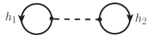
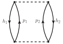
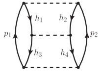
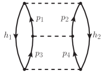
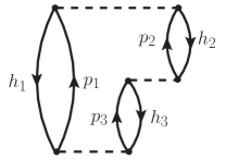
Figure 1: The first-, second-, and third-order ASG diagrams of energy corrections in the RS expansion Coraggio et al. (2003).

Fig. 1 displays the ASG diagrams corresponding to the first-, second- and third-order corrections to the energy in RSPT. The vertices, i.e., the dashed lines, represent $\hat{H}$ in Eq. (1). The diagrams (a) and (b) are for $E^{(1)}$ and $E^{(2)}$, respectively, while the diagrams (c), (d) and (e) sum up for $E^{(3)}$. The zero-order energy $E^{(0)}$ is the simple summation of the HF single-particle energies up to the Fermi level, i.e., $E^{(0)}=\displaystyle\sum_{i=1}^{A}\varepsilon_{i}$, where $\varepsilon_{i}$ represents the HF single-particle energy. The summation of the $E^{(0)}$ and $E^{(1)}$ gives the HF energy, i.e., $E_{\text{HF}}=E^{(0)}+E^{(1)}=\dfrac{1}{2}\displaystyle\sum_{i=1}^{A}\varepsilon_{i}$, since the initial Hamiltonian is entirely expressed in relative coordinates Bozzolo et al. (1988); Hasan et al. (2004).

II.4.1 Corrections to the one-body density

MBPT corrections to the wave function bring configuration mixing. The convergence can be discussed in order-by-order perturbation calculations. Any observable that is expressed by one-body operators can be calculated by using the One-Body Density Matrix (OBDM). By definition, the local one-body density operator in an $A$-body Hilbert space is written as Cockrell et al. (2012)

$$\hat{\rho}(\vec{r})=\displaystyle\sum_{k=1}^{A}\delta^{3}\left(\vec{r}-\vec{r}_{k}\right)=\displaystyle\sum_{k=1}^{A}\frac{\delta\left(r-r_{k}\right)}{r^{2}}\displaystyle\sum_{lm}Y_{lm}^{\ast}(\text{\^{r}}_{k})Y_{lm}(\text{\^{r}}),$$ (25)

where r̂ is the unit vector in the direction $\vec{r}$, and $Y_{lm}(\text{\^{r}})$ is the spherical harmonic function.

We can write the density operator in the second quantization representation in the HO basis as

$$\hat{\rho}(\vec{r})= \displaystyle\sum_{K}\displaystyle\sum_{n_{1}l_{1}j_{1}}\displaystyle\sum_{n_{2}l_{2}j_{2}}\displaystyle\sum_{m_{j}}R_{n_{1}l_{1}}(r)R_{n_{2}l_{2}}(r)\frac{-Y_{K0}^{\ast}(\text{\^{r}})}{\sqrt{2K+1}}$$ (26)

$$\times\left\langle l_{1}\frac{1}{2}j_{1}\left||Y_{K}|\right|l_{2}\frac{1}{2}j_{2}\right\rangle\left\langle j_{1}m_{j}j_{2}-m_{j}|K0\right\rangle$$

$$\times(-1)^{j_{2}+m_{j}}a_{n_{1}l_{1}j_{1}m_{j}}^{{\dagger}}a_{n_{2}l_{2}j_{2}m_{j}}$$

with

$$\left\langle l_{1}\frac{1}{2}j_{1}\left||Y_{K}|\right|l_{2}\frac{1}{2}j_{2}\right\rangle= \frac{1}{\sqrt{4\pi}}\text{\^{j}}_{1}\text{\^{j}}_{2}\text{\^{l}}_{1}\text{\^{l}}_{2}(-1)^{j_{1}+\frac{1}{2}}\left\langle l_{1}0l_{2}0|K0\right\rangle$$ (29)

$$\times\left\{\begin{array}[]{ccc}j_{1}&j_{2}&K\\ l_{2}&l_{1}&\frac{1}{2}\\ \end{array}\right\}.$$

The $R_{nl}$’s are the radial components of the HO wave function. We use the Condon-Shortley convention for the Clebsch-Gordan coefficients. Since we are dealing with a spherically symmetric system (K=0), we can obtain a simple form,

$$\hat{\rho}(\vec{r})=\displaystyle\sum_{n_{1}n_{2}}\displaystyle\sum_{ljm_{j}}\left[\frac{R_{n_{1}l}(r)R_{n_{2}l}(r)}{4\pi}\right]a_{n_{1}ljm_{j}}^{{\dagger}}a_{n_{2}ljm_{j}}.$$ (30)

By introducing the normally-ordered product relative to the SHF ground state $|\Phi_{0}\rangle$, the local one-body density operator can be written as

$$\hat{\rho}(\vec{r})=\rho_{0}(\vec{r})+\hat{\rho}_{N}=\rho_{0}(\vec{r})+\displaystyle\sum_{i,j}\rho_{ij}:c_{i}^{{\dagger}}c_{j}:,$$ (31)

where $\rho_{0}(\vec{r})=\langle\Phi_{0}|\hat{\rho}(\vec{r})|\Phi_{0}\rangle$ gives the HF density, while $\hat{\rho}_{N}=\displaystyle\sum_{i,j}\rho_{ij}:c_{i}^{{\dagger}}c_{j}:$ brings corrections to the density. $\rho_{ij}$ is the density matrix elements $\langle i|\rho(\vec{r})|j\rangle$, and $:c_{i}^{{\dagger}}c_{j}:$ indicates the normally-ordered product of the creation and annihilation operators. It is required that all annihilation and creation operators which take $|\Phi_{0}\rangle$ to zero when acting on it are to the right of all other operators which do not take $|\Phi_{0}\rangle$ to zero. The expectation value of the density is obtained with the corrected wave function through Eq. (31). In the present work, we consider the first- and second-order wave function corrections.

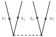
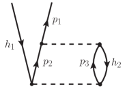
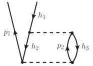
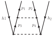
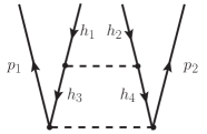
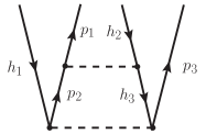
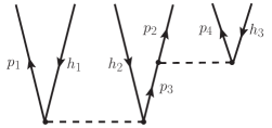
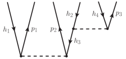
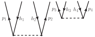
Figure 2: ASG diagrams for the first- and second-order corrections to the wave function Shavitt and Bartlett (2009). The panel (a) is for the first-order correction, while (b) (c) … (i) are for the second-order correction.

The ASG diagrams for the first- and second-order corrections to the wave function Shavitt and Bartlett (2009) are displayed in Fig. 2. The first-order wave function diagram, i.e., panel (a) in Fig. 2, produces the second-order correction to the density. While diagrams (b) and (c) of the second-order wave function correction produce second-order corrections to the density, other diagrams of the second-order wave function correction contribute to higher-order corrections to the density. The first- and second-order wave function corrections which correct the density up to the second order can be written as

$$\Psi^{(1)}= -\displaystyle\frac{1}{4}\displaystyle\sum_{h_{1}h_{2}}\displaystyle\sum_{p_{1}p_{2}}\frac{\langle p_{1}p_{2}|\text{\^{H}}|h_{1}h_{2}\rangle}{(\varepsilon_{h_{1}}+\varepsilon_{h_{2}}-\varepsilon_{p_{1}}-\varepsilon_{p_{2}})}$$ (32)

$$\times\left(c_{p_{1}}^{\dagger}c_{p_{2}}^{\dagger}c_{h_{2}}c_{h_{1}}|\Phi_{0}\rangle\right),$$

$$\Psi^{(2)}_{b}= \displaystyle\frac{1}{2}\displaystyle\sum_{h_{1}h_{2}}\displaystyle\sum_{p_{1}p_{2}p_{3}}\frac{\langle p_{1}h_{2}|\text{\^{H}}|p_{2}p_{3}\rangle\langle p_{2}p_{3}|\text{\^{H}}|h_{1}h_{2}\rangle}{(\varepsilon_{h_{1}}-\varepsilon_{p_{1}})(\varepsilon_{h_{1}}+\varepsilon_{h_{2}}-\varepsilon_{p_{2}}-\varepsilon_{p_{3}})}$$ (33)

$$\times\left(c_{p_{1}}^{\dagger}c_{h_{1}}|\Phi_{0}\rangle\right),$$

$$\Psi^{(2)}_{c}= -\displaystyle\frac{1}{2}\displaystyle\sum_{h_{1}h_{2}h_{3}}\displaystyle\sum_{p_{1}p_{2}}\frac{\langle h_{2}h_{3}|\text{\^{H}}|h_{1}p_{2}\rangle\langle p_{1}p_{2}|\text{\^{H}}|h_{2}h_{3}\rangle}{(\varepsilon_{h_{1}}-\varepsilon_{p_{1}})(\varepsilon_{h_{2}}+\varepsilon_{h_{3}}-\varepsilon_{p_{1}}-\varepsilon_{p_{2}})}$$ (34)

$$\times\left(c_{p_{1}}^{\dagger}c_{h_{1}}|\Phi_{0}\rangle\right).$$

The total wave function that corrects the density up to the second order is

$$\begin{array}[]{ll}\Psi=\Phi_{0}+\Psi^{(1)}+\Psi^{(2)}_{b}+\Psi^{(2)}_{c}.\end{array}$$ (36)

Then, the corrected density is written as

$$\rho(\vec{r}) =\langle\Psi|\hat{\rho}(\vec{r})|\Psi\rangle$$ (37)

$$=\langle\Phi_{0}|\hat{\rho}(\vec{r})|\Phi_{0}\rangle+\langle\Phi_{0}|\hat{\rho}(\vec{r})|\Phi_{0}\rangle\langle\Psi^{(1)}|\Psi^{(1)}\rangle$$

$$\quad+2\langle\Phi_{0}|\hat{\rho}_{N}|\Psi_{b}^{(2)}\rangle+2\langle\Phi_{0}|\hat{\rho}_{N}|\Psi_{c}^{(2)}\rangle+\langle\Psi^{(1)}|\hat{\rho}_{N}|\Psi^{(1)}\rangle$$

$$=\langle\Phi_{0}|\hat{\rho}(\vec{r})|\Phi_{0}\rangle+\langle\Phi_{0}|\hat{\rho}(\vec{r})|\Phi_{0}\rangle\langle\Psi^{(1)}|\Psi^{(1)}\rangle$$

$$\quad+2\rho_{a}+2\rho_{b}+\rho_{c_{1}}+\rho_{c_{2}},$$

where $\rho_{a}=\langle\Phi_{0}|\hat{\rho}_{N}|\Psi_{b}^{(2)}\rangle$, $\rho_{b}=\langle\Phi_{0}|\hat{\rho}_{N}|\Psi_{c}^{(2)}\rangle$ and $\rho_{c_{1}}+\rho_{c_{2}}=\langle\Psi^{(1)}|\hat{\rho}_{N}|\Psi^{(1)}\rangle$. They are displayed using the language of the diagram in Fig. 3. Dashed lines with cross contribute to the reduced matrix elements $\langle\nu_{1}lj\|\rho\|\nu_{2}lj\rangle=\sqrt{2j+1}\langle\nu_{1}ljm_{j}|\rho|\nu_{2}ljm_{j}\rangle$.

The detailed formulae of the density correction terms in the angular momentum coupled scheme are written as

$$\rho_{a}= \frac{1}{2}\displaystyle\sum_{h_{1},h_{2}}\displaystyle\sum_{p_{1},p_{2},p_{3}}\frac{(-1)^{j_{h_{1}}+j_{h_{2}}}\sqrt{2j_{h_{2}}+1}}{(\varepsilon_{h_{1}}-\varepsilon_{p_{1}})(\varepsilon_{h_{1}}+\varepsilon_{h_{2}}-\varepsilon_{p_{2}}-\varepsilon_{p_{3}})}$$

$$\times \displaystyle\sum_{J}(-1)^{J}(2J+1)\left\{\begin{array}[]{ccc}j_{h_{1}}&j_{p_{1}}&0\\ j_{h_{2}}&j_{h_{2}}&J\end{array}\right\}\langle(h_{1}h_{2})J|\text{\^{H}}|(p_{2}p_{3})J\rangle$$ (40)

$$\times \langle(p_{2}p_{3})J|\text{\^{H}}|(p_{1}h_{2})J\rangle\langle h_{1}\|\rho\|p_{1}\rangle,$$ (41)

$$\rho_{b}= -\frac{1}{2}\displaystyle\sum_{h_{1},h_{2},h_{3}}\displaystyle\sum_{p_{1},p_{2}}\frac{(-1)^{j_{h_{1}}+j_{p_{2}}}\sqrt{2j_{p_{2}}+1}}{(\varepsilon_{h_{1}}-\varepsilon_{p_{1}})(\varepsilon_{h_{2}}+\varepsilon_{h_{3}}-\varepsilon_{p_{1}}-\varepsilon_{p_{2}})}$$

$$\times \displaystyle\sum_{J}(-1)^{J}(2J+1)\left\{\begin{array}[]{ccc}j_{h_{1}}&j_{p_{1}}&0\\ j_{p_{2}}&j_{p_{2}}&J\end{array}\right\}\langle(p_{1}p_{2})J|\text{\^{H}}|(h_{2}h_{3})J\rangle$$ (44)

$$\times \langle(h_{2}h_{3})J|\text{\^{H}}|(h_{1}p_{2})J\rangle\langle h_{1}\|\rho\|p_{1}\rangle,$$ (45)

$$\rho_{c_{1}}= -\frac{1}{2}\displaystyle\sum_{h_{1},h_{2},h_{3}}\displaystyle\sum_{p_{1},p_{2}}\frac{(-1)^{j_{h_{1}}+j_{h_{2}}}\sqrt{2j_{h_{1}}+1}}{(\varepsilon_{h_{1}}+\varepsilon_{h_{2}}-\varepsilon_{p_{1}}-\varepsilon_{p_{2}})(\varepsilon_{h_{1}}+\varepsilon_{h_{3}}-\varepsilon_{p_{1}}-\varepsilon_{p_{2}})}$$

$$\times \displaystyle\sum_{J}(-1)^{J}(2J+1)\left\{\begin{array}[]{ccc}j_{h_{1}}&j_{h_{1}}&0\\ j_{h_{2}}&j_{h_{3}}&J\end{array}\right\}\langle(h_{1}h_{2})J|\text{\^{H}}|(p_{1}p_{2})J\rangle$$ (48)

$$\times \langle(p_{1}p_{2})J|\text{\^{H}}|(h_{1}h_{3})J\rangle\langle h_{3}\|\rho\|h_{2}\rangle,$$ (49)

$$\rho_{c_{2}}= \frac{1}{2}\displaystyle\sum_{h_{1},h_{2}}\displaystyle\sum_{p_{1},p_{2},p_{3}}\frac{(-1)^{j_{p_{1}}+j_{p_{3}}}\sqrt{2j_{p_{1}}+1}}{(\varepsilon_{h_{1}}+\varepsilon_{h_{2}}-\varepsilon_{p_{1}}-\varepsilon_{p_{3}})(\varepsilon_{h_{1}}+\varepsilon_{h_{2}}-\varepsilon_{p_{1}}-\varepsilon_{p_{2}})}$$

$$\times \displaystyle\sum_{J}(-1)^{J}(2J+1)\left\{\begin{array}[]{ccc}j_{p_{1}}&j_{p_{1}}&0\\ j_{p_{3}}&j_{p_{2}}&J\end{array}\right\}\langle(p_{1}p_{3})J|\text{\^{H}}|(h_{1}h_{2})J\rangle$$ (52)

$$\times \langle(h_{1}h_{2})J|\text{\^{H}}|(p_{1}p_{2})J\rangle\langle p_{2}\|\rho\|p_{3}\rangle,$$ (53)

where $\left\{\begin{array}[]{ccc}j_{1}&j_{2}&j_{3}\\ j_{4}&j_{5}&j_{6}\\ \end{array}\right\}$ is Wigner 6-j symbol. The letters $h_{1},h_{2},...$ indicate occupied single-particle levels in $|\text{HF}\rangle$ (i.e., hole states), the letters $p_{1},p_{2},...$ for unoccupied levels (i.e., particle states). $\varepsilon_{h}$ or $\varepsilon_{p}$ is the energy of particle or hole state, respectively. States $h$ or $p$ includes the quantum numbers of the orbital angular momentum $l$, total angular momentum $j$, isospin projection quantum number $m_{t}$, and additional quantum number $\nu$, i.e., $|h\rangle$ or $|p\rangle=|\nu ljt_{z}\rangle$. We define an anti-symmetrized two-particle state (unnormalized) coupled to a good angular momentum $J$ with a projection $M$,

$$|(j_{1}j_{2})JM\rangle=\displaystyle\sum_{m_{1},m_{2}}\langle j_{1}m_{1}j_{2}m_{2}|JM\rangle|(j_{1}m_{1})(j_{2}m_{2})\rangle.$$ (54)

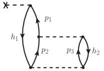
(a)  $\rho_{a}$

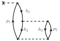
(b)  $\rho_{b}$

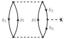
(c)  $\rho_{c_{1}}$

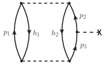
(d)  $\rho_{c_{2}}$

Figure 3: ASG diagrams for the second-order corrections to the density.

II.4.2 Root-mean-square radii

The root-mean-square (rms) radius is an important global indicator for the change of the density distribution arising from correlations beyond HF. The squares of the rms radii for point-like proton, neutron and nucleon (matter) distributions are the averaged values of the operators Kamuntavičius (1997), respectively,

$$\begin{array}[]{ll}{\hat{r}_{\text{pp}}}^{2}=\displaystyle\frac{1}{Z}\displaystyle\sum_{i=1}^{Z}(\vec{r_{i}}-\vec{r_{0}})^{2},\end{array}$$ (56)

$$\begin{array}[]{ll}{\hat{r}_{\text{nn}}}^{2}=\displaystyle\frac{1}{N}\displaystyle\sum_{i=1}^{N}(\vec{r_{i}}-\vec{r_{0}})^{2},\end{array}$$ (58)

$$\begin{array}[]{ll}{\hat{r}_{\text{m}}}^{2}=\displaystyle\frac{1}{A}\displaystyle\sum_{i=1}^{A}(\vec{r_{i}}-\vec{r_{0}})^{2}=\frac{1}{A^{2}}\displaystyle\sum_{i<j}^{A}(\vec{r_{i}}-\vec{r_{j}})^{2},\end{array}$$ (60)

with the c.m. position $\vec{r_{0}}=\frac{1}{A}\displaystyle\sum_{i=1}^{A}\vec{r_{i}}$. The charge radius $r_{\text{ch}}$ obtained from the point-proton radius $r_{\text{pp}}$ using the standard expression Ekström et al. (2015)

$$\langle r_{\text{ch}}^{2}\rangle=\langle r_{\text{pp}}^{2}\rangle+R_{\text{p}}^{2}+\dfrac{N}{Z}R_{\text{n}}^{2}+\dfrac{3\hbar^{2}}{4m_{\text{p}}^{2}c^{2}},$$ (61)

where $\dfrac{3\hbar^{2}}{4m_{\text{p}}^{2}c^{2}}\approx 0.033\;\text{fm}^{2}$, $R_{\text{n}}^{2}=-0.1149(27)\;\text{fm}^{2}$, $R_{\text{p}}=0.8775(51)$ fm. The point-proton or point-neutron rms radius operator is a two-body operator. The squares of the rms radii can be calculated either from the translational invariant local density or directly using the two-body operators [ i.e., Eqs. (56), (58) and (60) ]. Since we adopt MBPT with intermediate normalization [ i.e., Eqs. (17) ], the perturbed wave function is unnormalized. In the present work, we use the one-body local density to calculate the radius, as

$$\langle{R^{2}_{\text{pp}}}\rangle=\displaystyle\frac{\int r^{2}\rho_{\text{p}}(\vec{r})d^{3}r}{\int\rho_{\text{p}}(\vec{r})d^{3}r}.$$ (62)

The wave function is written in the laboratory HO coordinate, starting from an anti-symmetrized Slater determinant which contains the component of the center-of-mass (c.m.) motion. Consequently, the local one-body density calculated with the wave function includes contribution from the c.m. motion. The c.m. correction to the radius can be approximated as follows. Eq. (60) gives

$$\begin{array}[]{ll}{\hat{r}_{\text{m}}}^{2}=\displaystyle\frac{1}{A^{2}}\displaystyle\sum_{i<j}^{A}(\vec{r_{i}}-\vec{r_{j}})^{2}=\left(1-\frac{1}{A}\right)\cdot\left({\displaystyle\sum_{i=1}^{A}\vec{r_{i}}^{2}}/{A}\right)-\frac{2}{A^{2}}\cdot\left(\displaystyle\sum_{i<j}^{A}\vec{r_{i}}\cdot\vec{r_{j}}\right).\end{array}$$ (64)

If the cross term $\displaystyle\sum_{i<j}^{A}\vec{r_{i}}\cdot\vec{r_{j}}$ is neglected, we have

$$\begin{array}[]{ll}{\hat{r}_{\text{m}}}^{2}\approx\left(1-\displaystyle\frac{1}{A}\right)\cdot\left({\displaystyle\sum_{i=1}^{A}\vec{r_{i}}^{2}}/{A}\right)\end{array}.$$ (66)

Similarly for the proton radius,

$$\begin{array}[]{ll}{\hat{r}_{\text{pp}}}^{2}\approx\left(1-\displaystyle\frac{1}{A}\right)\cdot\left({\displaystyle\sum_{i=1}^{Z}\vec{r_{i}}^{2}}/{Z}\right)\end{array}.$$ (68)

This gives an approximate c.m. correction to the point-proton rms radius,

$$\begin{array}[]{ll}\Delta r_{\text{c.m.}}=\left[\left(1-\displaystyle\frac{1}{A}\right)\cdot\langle R_{\text{pp}}^{2}\rangle\right]^{1/2}-\langle R_{\text{pp}}^{2}\rangle^{1/2},\end{array}$$ (70)

where $\langle R_{\text{pp}}^{2}\rangle^{1/2}$ is the point-proton rms radius calculated by Eq (62). Then the rms radius of the point-proton distribution is obtained by

$$r_{\text{pp}}=\langle R_{\text{pp}}^{2}\rangle^{1/2}+\Delta r_{\text{c.m.}}.$$ (71)

III Calculations and discussions

In this section, we apply the method outlined in Section II to two light closed-shell nuclei, ⁴He and ¹⁶O. The SRG-softened chiral N³LO and the “bare” JISP16 interactions are adopted for the effective Hamiltonians.

III.1 Calculations with chiral N³LO interaction

The SHF is carried out within the HO basis. The HO basis is truncated by a cutoff according to the number $N_{\rm shell}=\text{max}(2n+l+1)$, where $N_{\rm shell}$ indicates how many major HO shells are included in the truncation. After the SHF calculation, the MBPT corrections are calculated in the SHF basis. In the present calculations, the basis spaces employed take $N_{\rm shell}$=7, 9, 11 and 13. We verify that such a truncation is sufficient for the converged calculations of the ground state energies for these magic nuclei ⁴He and ¹⁶O.

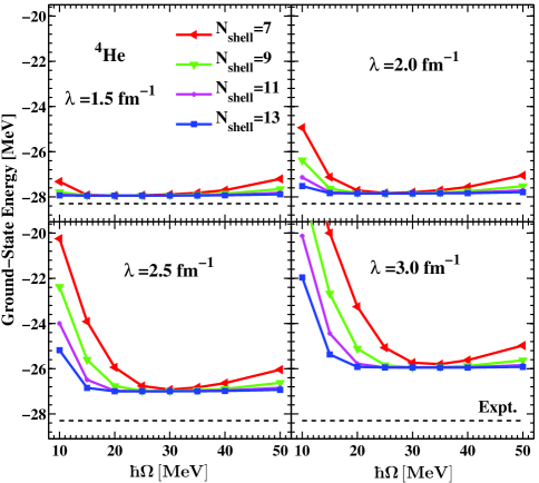
Figure 4: HF-MBPT calculations of ${}^{4}\text{He}$ ground-state energy through third order as a function of oscillator parameter $\hbar\Omega$ with the chiral N³LO potential Entem and Machleidt (2003); Machleidt and Entem (2011) renormalized by SRG at different softening parameters $\lambda=1.5,2.0,2.5,3.0$ $\text{fm}^{-1}$. The dashed line represents the experimental ground-state energy.

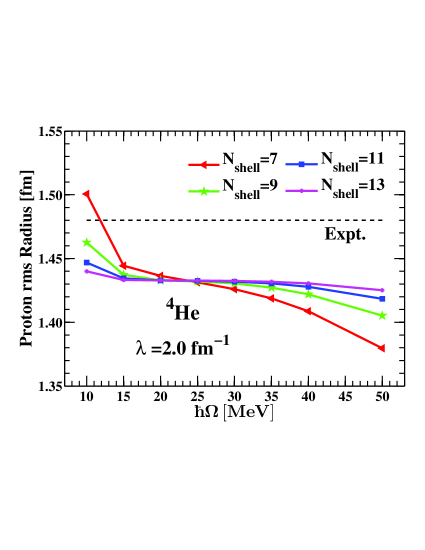
Figure 5: Point-proton rms radius of ⁴He as a function of oscillator parameter $\hbar\Omega$ with different $N_{\text{shell}}$. The chiral N³LO potential Entem and Machleidt (2003); Machleidt and Entem (2011) is softened by the SRG method.

Table 1: Ground-state energy (in MeV) of ⁴He, analyzed in order-by-order HF-MBPT calculations with N³LO softened at different SRG-softening parameter values ($\lambda$). PT2 and PT3 represent the second- and third-order corrections to energy, respectively. We take $N_{\text{shell}}=13$ and $\hbar\Omega=35$ MeV.

	SRG flow parameter $\lambda$ (fm-1)
	1.5	2.0	2.5	3.0
Expt. Audi et al. (2012)	-28.296	-28.296	-28.296	-28.296
NCSM  Jurgenson et al. (2013)	-28.20	-28.41	-27.43	-26.80
SHF	-25.754	-21.864	-15.854	-10.278
PT2	-1.788	-5.088	-9.652	-13.783
PT3	-0.391	-0.899	-1.523	-1.953
SHF+PT2+PT3	-27.933	-27.850	-27.029	-26.013

Table 2: Point-proton rms radius (in fm) of ⁴He in the HF-MBPT calculations with N³LO softened at different SRG-softening parameter values. PT2 designates the second-order correction to the radius. $N_{\text{shell}}=13$ and $\hbar\Omega=35$ MeV are taken. The experimental point-proton rms radius is obtained using Eq. (61) with the experimental charge radius taken from Angeli and Marinova (2013).

	SRG flow parameter $\lambda$ (fm-1)
	1.5	2.0	2.5	3.0
Expt.	1.477	1.477	1.477	1.477
SHF	1.677	1.652	1.714	1.816
PT2	0.007	0.001	-0.021	-0.065
$\Delta r_{\text{c.m.}}$	-0.226	-0.222	-0.227	-0.235
SHF+PT2+$\Delta r_{\text{c.m.}}$	1.458	1.431	1.466	1.516

Fig. 4 shows the MBPT calculated ground-state energy of ⁴He. The calculations were done with the chiral N³LO interaction which was renormalized by SRG. We see that good convergence of the calculated energy by virtue of independence from the oscillator parameter $\hbar\Omega$ and $N_{\text{shell}}$ is obtained at least for the truncations $N_{\text{shell}}=11$ and 13. We note that the dependence on the parameter $\hbar\Omega$ displays behavior similar to NCSM calculations Bogner et al. (2008); Jurgenson et al. (2013). The softening parameter $\lambda=3.0$ fm^-1 seems to be insufficient to produce an interaction soft enough for good convergence in MBPT. Jurgenson et al., have investigated the SRG evolution with the softening parameter $\lambda$ in ⁴He at $\hbar\Omega=36$ MeV Jurgenson et al. (2009, 2013). They found that $\lambda\approx 2.0$ fm^-1 can reasonably reproduce the experimental ⁴He ground-state energy with the $NN$-only interaction (without requiring a three-body force).

Fig. 5 shows the radius calculations at different $\hbar\Omega$ with $\lambda=2.0$ fm^-1. Tables 1 and  2 give the details of the HF-MBPT calculations with different $\lambda$ values. We see that both second- and third-order corrections to energy decrease with decreasing $\lambda$. This is easily understood because MBPT mainly treats intermediate-range correlations and these correlations are weakened with decreasing $\lambda$. With sufficiently small $\lambda$, higher-order corrections to the energy can be neglected. The second-order correction to the radius is already small, which decreases with decreasing $\lambda$ in ⁴He. The c.m. correction to the radius is larger than the MBPT correction. It may be concluded that, at least for ⁴He, MBPT corrections up to third order in energy and up to second order in radius within the HF basis should give converged results for $\lambda$ below about 3.0 fm^-1. It has been pointed out that the MBPT calculation within the HO basis could be divergent even for softened interactions Tichai et al. (2016). The Hamiltonian (1) is written already in the relative coordinate, and SHF can preserve the translational invariance for the ground state energy Schmid (2002) so that no c.m. correction is needed for the ground state energy.

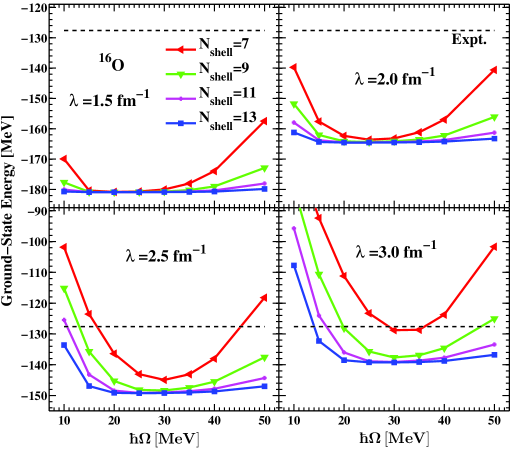
Figure 6: HF-MBPT calculations of ${}^{16}\text{O}$ as a function of oscillator parameter $\hbar\Omega$ with the chiral N³LO potential Entem and Machleidt (2003); Machleidt and Entem (2011) renormalized by SRG at different softening parameters $\lambda=1.5,2.0,2.5,3.0$ $\text{fm}^{-1}$.

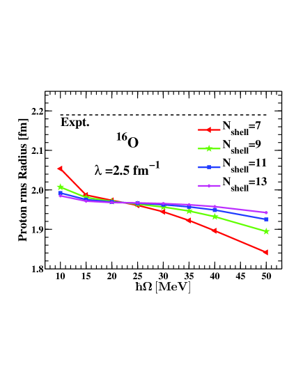
Figure 7: Point-proton rms radius of ¹⁶O as a function of oscillator parameter $\hbar\Omega$ with different $N_{\text{shell}}$. The chiral N³LO potential Entem and Machleidt (2003); Machleidt and Entem (2011) is softened by the SRG method.

Table 3: Ground-state energy (in MeV) of ¹⁶O, analyzed in order-by-order HF-MBPT calculations with N³LO softened at different SRG-softening parameter values ($\lambda$). We take $N_{\text{shell}}=13$ and $\hbar\Omega=35$ MeV.

	SRG flow parameter $\lambda$ (fm-1)
	1.5	2.0	2.5	3.0
Expt. Audi et al. (2012)	-127.619	-127.619	-127.619	-127.619
SHF	-169.968	-133.169	-85.173	-44.102
PT2	-10.132	-29.497	-59.617	-88.326
PT3	-0.794	-1.931	-4.630	-7.339
SHF+PT2+PT3	-180.893	-164.597	-149.419	-139.767

Table 4: Point-proton rms radius (in fm) of ¹⁶O in the HF-MBPT calculations with N³LO softened at different SRG-softening parameter values. $N_{\text{shell}}=13$ and $\hbar\Omega=35$ MeV are taken. The experimental point-proton rms radius is obtained using Eq. (61) with the experimental charge radius taken from Angeli and Marinova (2013).

	SRG flow parameter $\lambda$ (fm-1)
	1.5	2.0	2.5	3.0
Expt.	2.581	2.581	2.581	2.581
SHF	2.098	2.096	2.201	2.345
PT2	0.011	0.011	-0.006	-0.042
$\Delta r_{\text{c.m.}}$	-0.067	-0.067	-0.070	-0.073
SHF+PT2+$\Delta r_{\text{c.m.}}$	2.042	2.040	2.125	2.230

Fig. 6 shows the energy calculations for ¹⁶O. The convergence behavior is similar to that in ⁴He. The $N_{\rm shell}=11$ and 13 calculations appear nearly convergent. However, calculations with small $\lambda$ values (e.g., $\leq 2.0$ fm^-1) give over-binding, compared with data. This phenomenon should be more obvious for heavier nuclei. The main reason is that the three-body and higher-order forces are omitted in these calculations. The emergence of induced three-body forces and beyond is related to the SRG softening parameter $\lambda$. A larger $\lambda$ value evolves a harder effective $NN$ potential. In large $\lambda$ cases (e.g., $\lambda>3.0$ fm^-1), effects from induced three-body and higher-order forces are small. But a large $\lambda$ value may not sufficiently soften the short-range correlations of the realistic force, leading to demands for an excessively large model space and increased dependence on higher-order corrections. While a small $\lambda$ value may sufficiently soften the potential, the contribution from induced three-body force may be not ignorable. Within SRG, $\lambda\sim 2.0-2.5$ fm^-1 seems to be an optimal range in which the $NN$ interaction can be softened reasonably and the combined three-body (initial plus induced) effects are greatly reduced Jurgenson et al. (2013); Bogner et al. (2007); Tichai et al. (2016).

The calculation of the radius for ¹⁶O is displayed in Fig. 7. Reasonable convergence is obtained for $N_{\text{shell}}=11$ and 13. But the calculated radius is smaller than the experimental value. It seems that other ab initio results yield radii that are systematically smaller than experiment Roth et al. (2006); Ekström et al. (2015). In Tables 3 and  4, we give the order-by-order results of the HF-MBPT ¹⁶O calculations with the same parameters as those in ⁴He (i.e., $N_{\text{shell}}=13$ and $\hbar\Omega=35$ MeV) at different $\lambda$ values. The situation is similar to that in ⁴He. We can see that smaller contributions from the neglected higher-order corrections decrease with decreasing $\lambda$, and good convergence is obtained for the MBPT calculations within the HF basis at small $\lambda$ values. It has pointed out that in the HF basis the fourth- and higher-order MBPT corrections are known to be negligible in some cases Tichai et al. (2016).

III.2 Calculations with the “bare” JISP16 potential

As mentioned in the Introduction, the JISP16 interaction is established by the $J$-matrix technique, and its parameters were determined by fitting both $NN$ scattering data and nuclear structure data up to $A=16$ Shirokov et al. (2007). It is called “bare” because we, along with others, do not apply renormalization procedures in order to use it in nuclear structure calculations. To fit selected nuclear properties, the interaction has been tuned with phase-equivalent transformations to minimize the role of neglected many-body interactions. This tuning exploits the residual freedoms in the off-shell properties of the NN interaction Polyzou and Glöckle (1990).

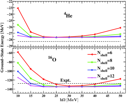
Figure 8: Ground-state binding energies of ⁴He and ¹⁶O as a function of the oscillator parameter $\hbar\Omega$ for different $N_{\text{shell}}$. The “bare” JISP16 potential Shirokov et al. (2004, 2005, 2007) is used. The dashed lines represent the experimental ground state energies.

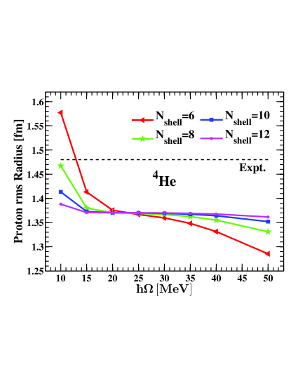
Figure 9: Point-proton rms radius of ⁴He as a function of the oscillator parameter $\hbar\Omega$ for different $N_{\text{shell}}$. The JISP16 potential Shirokov et al. (2004, 2005, 2007) is used.

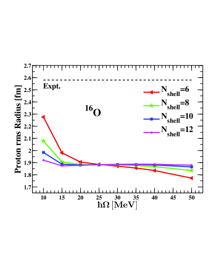
Figure 10: Point-proton rms radius of ¹⁶O as a function of the oscillator parameter $\hbar\Omega$ for different $N_{\text{shell}}$. The JISP16 potential Shirokov et al. (2004, 2005, 2007) is used.

Table 5: Ground-state binding energy and point-proton radius of ⁴He with the “bare” JISP16 interaction Shirokov et al. (2004, 2005, 2007) at $\hbar\Omega=35$ MeV. The results of HF-MBPT are obtained with $N_{\text{shell}}=10$. The NCSM results with $N_{\text{max}}=10$ are taken from Ref. Maris et al. (2009); Negoita (2010). The experimental energy is from Ref.Audi et al. (2012), and the experimental radius is obtained as in Table 2.

	Proton rms radius (fm)	$E_{\text{\text{g.s.}}}$ (MeV)
Expt.	1.477	$-28.296$
NCSM	$1.418$	$-28.222$
SHF	1.562	$-22.462$
PT2	0.015	$-4.373$
PT3	$-$	$-0.803$
$\Delta r_{\text{c.m.}}$	-0.211	$-$
HF-MBPT totally	1.366	$-27.638$

Table 6: Ground-state binding energy and point-proton radius of ¹⁶O with the “bare” JISP16 interaction Shirokov et al. (2004, 2005, 2007) at $\hbar\Omega=35$ MeV. The results of HF-MBPT are obtained with $N_{\text{shell}}=10$. The NCSM results with $N_{\text{max}}=8$ are taken from Ref. Maris et al. (2009); Negoita (2010). The experimental energy is from Ref. Audi et al. (2012), and the experimental radius is obtained as in Table 4.

	Proton rms radius (fm)	$E_{\text{g.s.}}$ (MeV)
Expt.	2.581	-127.619
NCSM	1.836	-131.091
SHF	1.852	-71.638
PT2	0.052	-58.873
PT3	$-$	-4.260
$\Delta r_{\text{c.m.}}$	-0.061	$-$
HF-MBPT totally	1.843	-134.771

Similar to the investigations with the chiral N³LO potential, we have applied the “bare” two-body JISP16 interaction to ⁴He and ¹⁶O. Figs. 8 show calculated binding energies for these two closed-shell nuclei. Figs. 9 and  10 are the radii calculations. Good convergence is obtained as indicated by the improved independence of $\hbar\Omega$ and $N_{\text{shell}}$ with increasing $N_{\text{shell}}$. The JISP16 potential without three-body force gives reasonable ground state energies compared with data. Tables 5 and  6 give the details of the HF-MBPT calculations with JISP16. To see how well the HF-MBPT approach does, we have made a comparison with the benchmark given by the NCSM calculation with the same JISP16 Maris et al. (2009); Negoita (2010). For the NCSM calculation, we introduce the model space truncation parameter $N_{max}$ that measures the maximal allowed HO excitation energy above the unperturbed lowest zero-order reference state. We choose to compare out results with $N_{max}$=10 for ⁴He calculations, impling that a total of 11 major HO shells are involved. Such a model space is sufficient for ⁴He. For the HF-MBPT calculation, fast convergence with increasing the size of the model space $N_{\text{shell}}$ has been shown in Fig. 8. We use the results of HF-MBPT with $N_{\text{shell}}$=10 to compare with the results of NCSM with $N_{\text{max}}=10$ as in Table 5. We see that HF-MBPT and NCSM calculations give similar results for the energy and radius of ⁴He, in good agreement with data. For ¹⁶O, we use $N_{\text{max}}$=8, which corresponds to a total of 10 major HO shells involved. The results of HF-MBPT with $N_{\text{shell}}$=10 truncation is used to compare with the NCSM results as in Table 6. Both HF-MBPT and the NCSM give larger binding energies but smaller radii than experimental data. The MBPT convergence with perturbative order in the “bare” JISP16 calculation is similar to that in the chiral N³LO calculation. With the calculations based on N³LO and JISP16, we may conclude that the MBPT method can give fairly converged results in the HF single-particle basis for these realistic $NN$ interactions.

IV Summary

We have performed the HF-MBPT calculations with the realistic $NN$ interactions chiral N³LO and “bare” JISP16. The detailed formulation and anti-symmetrized Goldstone diagram expansions are given. While the bare N³LO potential is softened using the SRG method, the “bare” JISP16 is employed without softening.. The MBPT corrections are performed based on the spherical Hartree-Fock approach. The spherical symmetry preserves the quantum numbers of angular momenta. The angular momentum coupled scheme can significantly reduce the model dimension and save the computational resources. As an improvement, we correct the one-body density for the calculation of the radius using anti-symmetrized Goldstone diagram expansions through second order.

The closed-shell nuclei, ⁴He and ¹⁶O, have been chosen as examples for the present HF-MBPT calculations. Convergence with respect to the SRG-softening parameter, harmonic oscillator frequency and model space truncation have been discussed in detail. Our results are consistent with other works published with MBPT or with other ab initio methods. We discussed the MBPT convergence order by order, showing that corrections up to the third order in energy and up to the second order in radius appear to be reasonable when one performs the HF-MBPT calculations within the Hartree-Fock single-particle basis. It is demonstrated that smaller contributions from the neglected higher orders decrease with decreasing SRG-softening parameter $\lambda$. In the present calculations, three-body and higher-order forces are not considered. To check the convergence of the MBPT calculation, we have made comparisons with benchmarks given by NCSM calculations with the same $NN$ potential. Consistent results have been obtained. In general, the calculated radii are smaller than experimental values, which is a common problem in current ab initio calculations with these interactions..