Helmholtz equation in a semi-infinite strip with impedance boundary conditions of the third and fifth orders

Abstract

Two boundary value problems for the Helmholtz equation in a semi-infinite strip are considered. The main feature of these problems is that, in addition to the function and its normal derivative on the boundary, the functionals of the boundary conditions possess tangential derivatives of the second and fourth orders. Also, the setting of the problems is complimented by certain edge conditions at the two vertices of the semi-strip. The problems model wave propagation in a semi-infinite waveguide with membrane and plate walls. A technique for the exact solution of these fluid-structure interaction problems is proposed. It requires application of two Laplace transforms with respect to both variables with the parameter of the second transform being a certain function of the first Laplace transform parameter. Ultimately, this method yields two scalar Riemann-Hilbert problems with the same coefficient and different right-hand sides. The dependence of the existence and uniqueness results of the physical model problems on the index of the Riemann-Hilbert problem is discussed.

1 Introduction

Boundary value problems for the Helmholtz equation with order $n\geq 2$ derivatives in the boundary conditions have been employed in the theory of diffraction since the work [1], where the second order derivatives on the boundary were used to model the surfaces of highly conducted materials. The first order impedance boundary conditions were generalized in [2] by adding second order tangential derivatives on the surface in order to model metal-backed dielectric layers. Order $n\geq 3$ boundary and transition conditions in electromagnetic diffraction theory were systematically studied in [3].

Higher order tangential derivatives in the boundary conditions naturally arise in model problems of aerodynamic noise theory and underwater acoustics when sound waves in fluids interact with flexible surfaces of waveguides [4]. Exact solutions and their analysis are available [5] for problems on a compressible fluid bounded by an infinite membrane and an elastic plate fixed along two or more parallel lines when the system is excited by an incident plane wave. These models for membranes and elastic plates are governed by the Helmholtz equation with the third and fifth order derivatives in the boundary conditions, respectively. The Wiener-Hopf method was applied in [6] to study the motion of an infinite plane composed of two half-planes with different elastic constants due to hydroacoustic pressure in the fluid beneath the plate. Edge diffraction of an incident acoustic plane wave by a thin elastic half-plane was treated in [7]. Due to the geometry of the model problem it was also solved by the Wiener-Hopf method.

For more complicated domains like a wedge, two joint wedges, or a semi-infinite strip whose boundaries are composed of either membranes or elastic plates the Wiener-Hopf method is not applicable. The Buchwald method [8] proposed for the solution of the model problem on diffraction of Kelvin waves at a corner was further developed [9] to study diffraction of acoustic waves in a semi-infinite waveguide whose surface is formed by elastic plates. In this work the authors determined that the number of free constants to be determined from the conditions at the vertices of the structure depends only on the orders of the derivatives in the boundary conditions. They also found an integral representation of the acoustic pressure distribution. Some model problems of sound-structure interaction with high-order boundary conditions by the method of eigenfunction expansions were treated in [10]. These include the problem of propagation of an acoustic wave in a semi-infinite waveguide when the upper boundary is a semi-infinite membrane, while the lower and the finite vertical sides are acoustically rigid walls (in this case, by symmetry, the problem for a a half-strip reduces to a problem for an infinite strip).

The Poincaré boundary value problem for the modified Helmholtz operator $\Delta-k^{2}$ ($k$ is a real number) in a semi-infinite strip was studied in [11] by the method proposed in [12]. It was shown that the problem reduces to an order-2 vector Riemann-Hilbert problem on the real axis whose matrix coefficient, in general, does not admit an explicit factorization by the methods currently available in the literature. However, in some important cases, including the case of impedance boundary conditions, it allows for an exact factorization and in some other cases the vector problem reduces to a problem with triangle matrix coefficient, or could be even decoupled. Notice that in the case of the Helmholtz operator $\Delta+k^{2}$ ($k\in{{R}}$), the contour of the Riemann-Hilbert problem comprises two semi-infinite rays and two circular arcs.

Our goal in this work is to develop an efficient method for the Helmholtz equation in a semi-infinite strip $\{0<x<\infty,0<y<a\}$ with generalized impedance boundary conditions of higher order. The main feature of this technique is that it applies two Laplace transforms in a nonstandard way. The first transform is utilized with respect to $x$ in the classical way, while the second one is applied in the $y$-direction (the function is extended by zero for $y>a$) with a parameter $\zeta$ that is a root of the characteristic polynomial of the ordinary differential operator $d^{2}/dy^{2}+k^{2}-\eta^{2}$, the Laplace image of the original Helmholtz operator. This root is $\zeta=\sqrt{\eta^{2}-k^{2}}$, where $k$ is the wave number, $\eta$ is the parameter of the first transform, and $\sqrt{\eta^{2}-k^{2}}$ is a fixed branch of the function $\zeta^{2}=\eta^{2}-k^{2}$. The method to be proposed ultimately yields two symmetric scalar Riemann-Hilbert problems on the real axis equivalent to the original model problem. We emphasize that the contour is the real axis regardless if $k$ is real, imaginary, or a general complex number. The Riemann-Hilbert problems share the same coefficient and have different right-hand sides. Remarkably, the coefficient is a simple rational function, $G(\eta)=P_{n}(\eta)/P_{n}(-\eta)$, where the degree of the polynomial $P_{n}(\eta)$ is $n=3$ (in the membrane case) and $n=5$ (in the elastic plate case) and coincide with the order of the highest derivative involved in the boundary conditions. We determine the number of free constants in the solution that depends not only on the order of the tangential derivatives in the boundary conditions but also on the position of the zeros of the polynomial $P_{n}(\eta)$ and therefore the parameters of the problem. Also, we derive explicitly a system of linear algebraic equations for the unknown constants and summarize the results by stating an existence - uniqueness theorem. Finally, we write down representation formulas for the solution by quadratures and, in addition, by series convenient for computational purposes.

2 Helmholtz equation in a semi-infinite waveguide: membrane walls

2.1 Formulation

Of concern is the Helmholtz equation

$$\left(\frac{\partial^{2}}{\partial x^{2}}+\frac{\partial^{2}}{\partial y^{2}}+k^{2}\right)u(x,y)=g(x,y),\quad 0<x<\infty,\quad 0<y<a,$$ (2.1)

with respect to an unknown function $u(x,y)$ subjected to the boundary conditions

$$\left[\left(\frac{\partial^{2}}{\partial x^{2}}+\alpha_{0}^{2}\right)\frac{\partial}{\partial y}-\mu_{0}\right]u=g_{0}(x),\quad(x,y)\in W_{0}=\{0<x<\infty,\;y=0\},$$

$$\left[\left(\frac{\partial^{2}}{\partial x^{2}}+\alpha_{1}^{2}\right)\frac{\partial}{\partial y}+\mu_{1}\right]u=g_{1}(x),\quad(x,y)\in W_{1}=\{0<x<\infty,\quad y=a\},$$

$$\left[\left(\frac{\partial^{2}}{\partial y^{2}}+\alpha_{2}^{2}\right)\frac{\partial}{\partial x}-\mu_{2}\right]u=g_{2}(y),\quad(x,y)\in W_{2}=\{x=0,\quad 0<y<a\}.$$ (2.2)

This boundary value problem governs acoustic wave propagation in a semi-infinite waveguide (Fig.1).

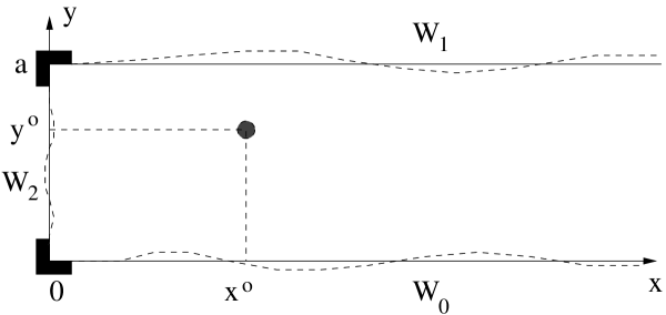
Figure 1: Geometry of the problem on a semi-infinite waveguide.

Here, $\mathop{\rm Re}\nolimits[e^{-i\omega t}u(x,y)]$ is the fluid velocity potential, $\omega$ is the frequency, $\omega=\omega_{1}+i\omega_{2}$, $\omega_{j}>0$, $t$ is time, $k=\omega/c$ is the wave number, $c$ is the sound speed in the fluid. The pressure distribution $p(x,y)$ and the deflection of the horizontal and vertical walls, $u_{0}(x)$, $u_{1}(x)$, and $u_{2}(y)$, are expressed through the velocity potential as

$$p(x,y)=i\omega\rho u(x,y),\quad u_{j}(x)=\frac{i}{\omega}u_{y}(x,y_{j}),\quad u_{2}(y)=\frac{i}{\omega}u_{x}(0,y),$$ (2.3)

where $j=0,1$, $y_{0}=0$, $y_{1}=a$, $\rho$ is the mean fluid density, and the suffixes $x$ and $y$ denote differentiation with respect to $x$ and $y$, respectively, The boundary conditions (2.2) model the deflection of the membrane walls due to pressure loading (Leppington, 1978). The parameters involved are

$$\alpha_{j}=\omega\sqrt{\frac{m_{j}}{T_{j}}},\quad\mu_{j}=\frac{\rho\omega^{2}}{T_{j}},\quad j=0,1,2,$$ (2.4)

where $m_{j}$ is the mass per unit area, and $T_{j}$ is the surface tension for the membrane $W_{j}$. Since $\mathop{\rm Im}\nolimits\omega>0$, we have $\mathop{\rm Im}\nolimits\alpha_{j}>0$. The functions $g(x,y)$, $g_{0}(x)$, $g_{1}(x)$, and $g_{2}(y)$ are prescribed. They will be later selected as $g_{0}(x)=g_{1}(x)=0$, $0<x<\infty$, $g_{2}(y)=0$, $0<y<a$, and $g(x,y)=-\delta(x-x^{\circ})\delta(y-y^{\circ})$, $(x^{\circ},y^{\circ})$ is an internal point of the semi-strip, and $\delta(\cdot)$ is the Dirac function. We also need to specify the edge conditions at $x=y=0$ and $x=0$, $y=a$. It is assumed that the edges are fixed, and therefore the following four conditions have to be satisfied:

$$\lim_{x\to 0^{+}}u_{y}(x,0)=\lim_{x\to 0^{+}}u_{y}(x,a)=0,$$

$$\lim_{y\to 0^{+}}u_{x}(0,y)=\lim_{y\to a^{-}}u_{x}(0,y)=0.$$ (2.5)

2.2 Two scalar Riemann-Hilbert problems

Our goal in this section is to present a method that is capable to convert the boundary value problem for the Helmholtz equation (2.1) with higher-order boundary conditions (2.2) in a semi-strip to two scalar Riemann-Hilbert problems. To achieve this, we apply first the Laplace transform with respect to $x$

$$\tilde{u}(\eta,y)=\int_{0}^{\infty}u(x,y)e^{i\eta x}dx$$ (2.6)

to equation (2.1) and the first and second boundary conditions in (2.2). In conjunction with (2.5) this brings us to the one-dimensional boundary value problem

$$L[\tilde{u}]\equiv\left(\frac{d^{2}}{dy^{2}}-\zeta^{2}\right)\tilde{u}(\eta,y)=f(y),\quad 0<y<a,$$

$$U_{0}[\tilde{u}]\equiv-\tilde{u}_{y}(\eta,0)+\tilde{\mu}_{0}(\eta)\tilde{u}(\eta,0)=\tilde{g}^{0}(\eta),$$

$$U_{1}[\tilde{u}]\equiv\tilde{u}_{y}(\eta,a)+\tilde{\mu}_{1}(\eta)\tilde{u}(\eta,a)=\tilde{g}^{1}(\eta),$$ (2.7)

where

$$\zeta^{2}=\eta^{2}-k^{2},\quad f(y)=u_{x}(0,y)-i\eta u(0,y)+\tilde{g}(\eta,y),$$

$$\tilde{\mu}_{j}=\frac{\mu_{j}}{\alpha_{j}^{2}-\eta^{2}},\quad\tilde{g}^{j}(\eta)=(-1)^{j+1}\frac{\tilde{g}_{j}(\eta)+c_{j}}{\alpha_{j}^{2}-\eta^{2}},$$

$$\tilde{g}(\eta,y)=\int_{0}^{\infty}g(x,y)e^{i\eta x}dx,\quad\tilde{g}_{j}(\eta)=\int_{0}^{\infty}g_{j}(x)e^{i\eta x}dx,\quad j=0,1,$$ (2.8)

and $c_{0}$ and $c_{1}$ are unknown constants

$$c_{0}=u_{xy}(0^{+},0),\quad c_{1}=u_{xy}(0^{+},a).$$ (2.9)

These constants and the functions $u_{x}(0,y)$ and $u(0,y)$ in (2.8) are to be determined.

Denote by $\zeta=\sqrt{\eta^{2}-k^{2}}$ the single branch of the two-valued function $\zeta^{2}=\eta^{2}-k^{2}$ in the $\eta$-plane cut along the straight line joining the branch points $\eta=\pm k$ ($k\in{{C}}^{+}$) and passing through the infinite point; the branch is fixed by the condition $\zeta=-ik$ as $\eta=0$. We next employ the Green function of the boundary value problem (2.7)

$$G(y,s)=-\frac{e^{-\zeta|y-s|}}{2\zeta}+\frac{1}{2\zeta\tilde{\Delta}(\zeta)}\left\{(\tilde{\mu}_{0}-\zeta)[\zeta\cosh\zeta(a-y)+\tilde{\mu}_{1}\sinh\zeta(a-y)]e^{-\zeta s}\right.$$

$$\left.+(\tilde{\mu}_{1}-\zeta)(\zeta\cosh\zeta y+\tilde{\mu}_{0}\sinh\zeta y)e^{-\zeta(a-s)}\right\},$$ (2.10)

and the fundamental system, namely the two solutions $\phi_{0}(y)$ and $\phi_{1}(y)$ of the problem

$$L[\phi_{j}(y)]=0,\quad 0<y<a,$$

$$U_{m}[\phi_{j}]=\delta_{mj},\quad m,j=0,1,$$ (2.11)

which are

$$\phi_{0}(y)=\frac{\zeta\cosh\zeta(a-y)+\tilde{\mu}_{1}\sinh\zeta(a-y)}{\tilde{\Delta}(\zeta)},\quad\phi_{1}(y)=\frac{\zeta\cosh\zeta y+\tilde{\mu}_{0}\sinh\zeta y}{\tilde{\Delta}(\zeta)}.$$ (2.12)

Here,

$$\tilde{\Delta}(\zeta)=(\tilde{\mu}_{0}+\tilde{\mu}_{1})\zeta\cosh a\zeta+(\tilde{\mu}_{0}\tilde{\mu}_{1}+\zeta^{2})\sinh a\zeta.$$ (2.13)

In terms of the Green function and the functions $\phi_{0}$ and $\phi_{1}$ the solution of the problem (2.7) can be written as

$$\tilde{u}(\eta,y)=\int_{0}^{a}G(y,s)f(s)ds+\tilde{g}^{0}(\eta)\phi_{0}(y)+\tilde{g}^{1}(\eta)\phi_{1}(y).$$ (2.14)

Now, by putting $y=0$ and $y=a$ in this formula and denoting

$$\hat{u}(0,i\zeta)=\int_{0}^{a}u(0,y)e^{-\zeta y}dy,\quad\hat{u}_{x}(0,i\zeta)=\int_{0}^{a}u_{x}(0,y)e^{-\zeta y}dy,$$

$$\hat{\tilde{g}}(\eta,i\zeta)=\int_{0}^{a}\tilde{g}(\eta,y)e^{-\zeta y}dy,$$ (2.15)

we obtain two relations which can be complimented by their counterparts with $\eta$ being replaced by $-\eta$; the four resulting equations are

$$\tilde{u}(\pm\eta,0)+\Lambda_{00}(\zeta)\hat{u}_{x}(0,i\zeta)\mp i\eta\Lambda_{00}(\zeta)\hat{u}(0,i\zeta)$$

$$+\Lambda_{01}(\zeta)\hat{u}_{x}(0,-i\zeta)\mp i\eta\Lambda_{01}(\zeta)\hat{u}(0,-i\zeta)+h_{0}(\pm\eta)=0,$$

$$\tilde{u}(\pm\eta,a)+\Lambda_{10}(\zeta)\hat{u}_{x}(0,i\zeta)\mp i\eta\Lambda_{10}(\zeta)\hat{u}(0,i\zeta)$$

$$+\Lambda_{11}(\zeta)\hat{u}_{x}(0,-i\zeta)\mp i\eta\Lambda_{11}(\zeta)\hat{u}(0,-i\zeta)+h_{1}(\pm\eta)=0,$$ (2.16)

where

$$\Lambda_{00}(\zeta)=\frac{1}{2\zeta}\left[1-\frac{\tilde{\mu}_{0}-\zeta}{\tilde{\Delta}(\zeta)}(\zeta\cosh a\zeta+\tilde{\mu}_{1}\sinh a\zeta)\right],$$

$$\Lambda_{01}(\zeta)=-\frac{\tilde{\mu}_{1}-\zeta}{2\tilde{\Delta}(\zeta)}e^{-a\zeta},\quad\Lambda_{10}(\zeta)=-\frac{\tilde{\mu}_{0}-\zeta}{2\tilde{\Delta}(\zeta)},$$

$$\Lambda_{11}(\zeta)=\frac{e^{-a\zeta}}{2\zeta}\left[1-\frac{\tilde{\mu}_{1}-\zeta}{\tilde{\Delta}(\zeta)}(\zeta\cosh a\zeta+\tilde{\mu}_{0}\sinh a\zeta)\right].$$ (2.17)

and

$$h_{0}(\eta)=\Lambda_{00}(\zeta)\hat{\tilde{g}}(\eta,i\zeta)+\Lambda_{01}(\zeta)\hat{\tilde{g}}(\eta,-i\zeta)-\frac{(\zeta\cosh a\zeta+\tilde{\mu}_{1}\sinh a\zeta)\tilde{g}^{0}(\eta)}{\tilde{\Delta}(\zeta)}-\frac{\zeta\tilde{g}^{1}(\eta)}{\tilde{\Delta}(\zeta)},$$

$$h_{1}(\eta)=\Lambda_{10}(\zeta)\hat{\tilde{g}}(\eta,i\zeta)+\Lambda_{11}(\zeta)\hat{\tilde{g}}(\eta,-i\zeta)-\frac{\zeta\tilde{g}^{0}(\eta)}{\tilde{\Delta}(\zeta)}-\frac{(\zeta\cosh a\zeta+\tilde{\mu}_{0}\sinh a\zeta)\tilde{g}^{1}(\eta).}{\tilde{\Delta}(\zeta)}$$ (2.18)

We emphasize two points here. First, the relative simplicity of the relations (2.16) is due to the fact that the functions $\zeta(\eta)$, $\tilde{\mu}_{0}(\eta)$ and $\tilde{\mu}_{1}(\eta)$ are even, which in turn is a consequence of the absence of odd order derivatives in the Helmholtz operator and odd order tangential derivatives in the boundary conditions (2.2). The second point is that the relations (2.16) connect the $\pm\eta$-Laplace transforms of the functions $u(x,0)$ and $u(x,a)$ with the functions $\hat{u}(0,\pm i\zeta)$ and $\hat{u}_{x}(0,\pm i\zeta)$. If the function $u(0,y)$ and the derivative $u_{x}(0,y)$ are extended by zero to $y\in(a,\infty)$, then $\hat{u}(0,\pm i\zeta)$ and $\hat{u}_{x}(0,\pm i\zeta)$ are their Laplace transforms whose parameters are not arbitrary but functions of $\eta$, the parameter of the first Laplace transform (2.6). These functions of $\eta$ are the two zeros $\pm\zeta$ of the characteristic polynomial $r^{2}-\zeta^{2}$ of the differential operator $L$ in (2.7).

We assert that the boundary condition on the vertical side $M_{2}=\{x=0,0<y<a\}$ has not been satisfied yet. On extending the function $g_{2}(y)$ by zero to the interval $y>a$, applying the Laplace transform to the third condition in (2.2) with the parameters $\zeta$ and $-\zeta$ and utilizing the edge conditions (2.5) we discover

$$-\hat{u}_{x}(0,\pm i\zeta)+\hat{\mu}_{2}(\zeta)\hat{u}(0,\pm i\zeta)=\hat{g}^{2}(\pm i\zeta),$$ (2.19)

where

$$\hat{\mu}_{2}(\zeta)=\frac{\mu_{2}}{\zeta^{2}+\alpha_{2}^{2}},\quad\hat{g}^{2}(i\zeta)=\frac{-\hat{g}_{2}(i\zeta)-c_{2}+c_{3}e^{-a\zeta}}{\zeta^{2}+\alpha_{2}^{2}},$$

$$\hat{g}_{2}(i\zeta)=\int_{0}^{a}g_{2}(y)e^{-\zeta y}dy,$$ (2.20)

and $c_{2}$ and $c_{3}$ are unknown constants,

$$c_{2}=u_{xy}(0,0^{+}),\quad c_{3}=u_{xy}(0,a^{-}),$$ (2.21)

to be fixed.

Our intension next is to express the four functions $\hat{u}(0,\pm i\zeta)$ and $\hat{u}_{x}(0,\pm i\zeta)$ through the functions $\tilde{u}(\pm\eta,0)$ and $\tilde{u}(\pm\eta,a)$ from the system (2.16) and insert them into the two equations (2.19). We have first

$$\left(\begin{array}[]{c}\hat{u}_{x}(0,i\zeta)\\ \hat{u}(0,i\zeta)\\ \hat{u}_{x}(0,-i\zeta)\\ \hat{u}(0,-i\zeta)\\ \end{array}\right)=\Lambda(\zeta)\left(\begin{array}[]{c}\tilde{u}(\eta,0)+h_{1}(\eta)\\ \tilde{u}(-\eta,0)+h_{1}(-\eta)\\ \tilde{u}(\eta,a)+h_{2}(\eta)\\ \tilde{u}(-\eta,a)+h_{2}(-\eta)\\ \end{array}\right),$$ (2.22)

where

$$\Lambda(\zeta)=-\frac{1}{2\eta}\left(\begin{array}[]{cccc}\eta(\tilde{\mu}_{0}+\zeta)&\eta(\tilde{\mu}_{0}+\zeta)&\eta(\tilde{\mu}_{1}-\zeta)e^{-a\zeta}&\eta(\tilde{\mu}_{1}-\zeta)e^{-a\zeta}\\ i(\tilde{\mu}_{0}+\zeta)&-i(\tilde{\mu}_{0}+\zeta)&i(\tilde{\mu}_{1}-\zeta)e^{-a\zeta}&-i(\tilde{\mu}_{1}-\zeta)e^{-a\zeta}\\ \eta(\tilde{\mu}_{0}-\zeta)&\eta(\tilde{\mu}_{0}-\zeta)&\eta(\tilde{\mu}_{1}+\zeta)e^{a\zeta}&\eta(\tilde{\mu}_{1}+\zeta)e^{a\zeta}\\ i(\tilde{\mu}_{0}-\zeta)&-i(\tilde{\mu}_{0}-\zeta)&i(\tilde{\mu}_{1}+\zeta)e^{a\zeta}&-i(\tilde{\mu}_{1}+\zeta)e^{a\zeta}\\ \end{array}\right),$$ (2.23)

and then, after utilizing equations (2.19), we eventually arrive at the following remarkably simple scalar Riemann-Hilbert problems which share the same coefficient and have different free terms:

$$\Phi_{j}^{+}(\eta)=H(\eta)\Phi_{j}(\eta)+f_{j}(\eta),\quad-\infty<\eta<+\infty,$$ (2.24)

subject to the symmetry conditions

$$\Phi_{j}^{+}(\eta)=\Phi_{j}^{-}(-\eta),\quad\eta\in{{C}},\quad j=0,1,$$ (2.25)

where

$$\Phi_{0}^{\pm}(\eta)=\tilde{u}(\pm\eta,0),\quad\Phi_{1}^{\pm}(\eta)=\tilde{u}(\pm\eta,a),$$ (2.26)

and

$$H(\eta)=-\frac{\eta+i\hat{\mu}_{2}(\zeta)}{\eta-i\hat{\mu}_{2}(\zeta)}=-\frac{\eta(\eta^{2}-k^{2}+\alpha_{2}^{2})+i\mu_{2}}{\eta(\eta^{2}-k^{2}+\alpha_{2}^{2})-i\mu_{2}},$$

$$f_{j}(\eta)=-h_{j}(\eta)+H(\eta)h_{j}(-\eta)+\frac{\eta}{(\eta-i\hat{\mu}_{2})\tilde{\Delta}(\zeta)}$$

$$\times\{[\zeta+(-1)^{j}\tilde{\mu}_{1-j}]e^{(1-j)a\zeta}\hat{g}_{2}(i\zeta)+[\zeta-(-1)^{j}\tilde{\mu}_{1-j}]e^{(j-1)a\zeta}\hat{g}_{2}(-i\zeta)\},\quad j=0,1.$$ (2.27)

The functions $\Phi_{j}^{+}(\eta)$ and $\Phi_{j}^{-}(\eta)$ are analytically continued from the contour, the real axis, into the upper and lower half-planes, ${{C}}^{+}$ and ${{C}}^{-}$, respectively. Denote

$$q(\eta)=\eta(\eta^{2}-k^{2}+\alpha_{2}^{2})+i\mu_{2}.$$ (2.28)

Then $H(\eta)=q(\eta)/q(-\eta)$. It turns out that for all $k=k_{1}+ik_{2}$, $k_{j}\geq 0$, $k_{1}^{2}+k_{2}^{2}>0$, and all admissible values of the parameters $\alpha_{2}$ and $\mu_{2}$ introduced in (2.4), the zeros $z_{j}$ of the cubic polynomial $q(\eta)$ are simple, and we have the following three possibilities:

(i) $z_{0}=-\eta_{0}$, $z_{1}=\eta_{1}$, and $z_{2}=-\eta_{2}$, $\mathop{\rm Im}\nolimits\eta_{j}>0$, $j=0,1,2$,

(ii) $z_{0}=\eta_{0}$, $z_{1}=\eta_{1}$, and $z_{2}=-\eta_{2}$, $\mathop{\rm Im}\nolimits\eta_{0}=0$, $\mathop{\rm Im}\nolimits\eta_{j}>0$, $j=1,2$,

(iii) $z_{0}=\eta_{0}$, $z_{1}=\eta_{1}$, and $z_{2}=-\eta_{2}$, $\mathop{\rm Im}\nolimits\eta_{j}>0$, $j=0,1,2$.

Table 1. The roots $z_{j}$ $(j=0,1,2)$ of $q(\eta)=\eta(\eta^{2}-k^{2}+k^{2}\gamma_{0})+ik^{2}\gamma_{1}$ for some values of the parameters $\gamma_{0}$, $\gamma_{1}$, and $k$.

$\gamma_{0}$	$\gamma_{1}$	$k$	$z_{0}$	$z_{1}$	$z_{2}$
5	1	$1+0.1i$	$-0.0008424-0.2540i$	$-0.2009+2.115i$	$0.2017-1.861i$
0.5	0.1	$1+0.1i$	$0.7264-0.02424i$	$-0.002135+0.1872i$	$-0.7243-0.1629i$
1	0.1	$1+i$	$0.5848$	$-0.2924+0.5065i$	$-0.2924-0.5065i$
0.5	0.05	$1+0.1i$	$0.7123+0.02117i$	$-0.0003512+0.09816i$	$-0.7120-0.1193i$
1	0.1	$i$	$-0.4020+0.2321i$	$0.4020+0.2321i$	$-0.4642i$

In Table 1 we present the roots of the polynomial $q(\eta)$ in cases (i) (the first two rows), (ii) (the third row), and (iii) (the fourth and fifth rows). For convenience, we used the following notations: $\gamma_{0}=\alpha_{2}^{2}/k^{2}=m_{2}c^{2}/T_{2}$ and $\gamma_{1}=\mu_{2}/k^{2}=\rho c^{2}/T_{2}$.

Consider the first case when the polynomial $q(\alpha)$ has one zero in the upper half-plane and two zeros in the lower half-plane. The location of the zeros enables us to factorize the coefficient $H(\eta)$ as

$$H(\eta)=\frac{H^{+}(\eta)}{H^{-}(\eta)},\quad-\infty<\eta<+\infty,$$ (2.29)

where

$$H^{+}(\eta)=\frac{(\eta+\eta_{0})(\eta+\eta_{2})}{\eta+\eta_{1}},\quad H^{-}(\eta)=-\frac{(\eta-\eta_{0})(\eta-\eta_{2})}{\eta-\eta_{1}},$$ (2.30)

and $\pm\eta_{j}\in{{C}}^{\pm}$, $j=0,1,2$. The index (the winding number) of the function $H(\eta)$ equals -1, and in the class of functions having a simple zero at the infinite point one expects the Riemann-Hilbert problems being solvable if and only if a certain condition is fulfilled (Gakhov, 1966). However, we assert that in our case this condition is identically satisfied, and the solution always exists. This solution is unique provided the functions $f_{j}(\tau)$ are uniquely defined. Indeed, introduce the Cauchy integrals

$$\Psi_{j}^{\pm}(\eta)=\frac{1}{2\pi i}\int_{-\infty}^{\infty}\frac{f_{j}(\tau)d\tau}{H^{+}(\tau)(\tau-\eta)},\quad\eta\in{{C}}^{\pm},\quad j=0,1,$$ (2.31)

with the densities $f_{j}(\tau)/H^{+}(\tau)$ vanishing at the infinite point, and $|f_{j}(\tau)/H^{+}(\tau)|\leq c|\tau|^{-4}$, $\tau\to\pm\infty$, $c$ is a nonzero constant. The standard application of the continuity principle and the Liouville theorem brings us to the following representation formulas for the solution of the Riemann-Hilbert problems (2.27):

$$\Phi_{j}^{\pm}(\eta)=H^{\pm}(\eta)\Psi_{j}^{\pm}(\eta),\quad\eta\in{{C}}^{\pm},\quad j=0,1.$$ (2.32)

It is directly verified that

$$\frac{f_{j}(\tau)}{H^{+}(\tau)}=-\frac{f_{j}(-\tau)}{H^{+}(-\tau)},$$ (2.33)

and therefore (2.31) implies

$$\Psi_{j}^{\pm}(\eta)=\frac{1}{\pi i}\int_{0}^{\infty}\frac{f_{j}(\tau)}{H^{+}(\tau)}\frac{\tau d\tau}{\tau^{2}-\eta^{2}}=O\left(\frac{1}{\eta^{2}}\right),\quad\eta\in{{C}}^{\pm},\quad\eta\to\infty.$$ (2.34)

Clearly, the functions $\Phi_{0}^{\pm}(\eta)$ and $\Phi_{1}^{\pm}(\eta)$ have a simple zero at the infinite point as it is required. Due to the presence of the functions $f_{j}(\eta)$ they have four unknown constants $c_{m}$ ($m=0,1,2,3$).

Consider now case (ii) when one of the zeros of the polynomial $q(\eta)$, $z_{0}=\eta_{0}$, is real, and the other two, $z_{1}=\eta_{1}$ and $z_{2}=-\eta_{2}$, lie in the half-planes ${{C}}^{+}$ and ${{C}}^{-}$, respectively. Owing to this, we select the Wiener-Hopf factors in (2.29) as

$$H^{+}(\eta)=\frac{\eta+\eta_{2}}{(\eta+\eta_{0})(\eta+\eta_{1})},\quad H^{-}(\eta)=-\frac{\eta-\eta_{2}}{(\eta-\eta_{0})(\eta-\eta_{1})},$$ (2.35)

Upon representing the function $f_{j}(\eta)/H^{+}(\eta)$ as the difference $\Psi^{+}_{j}(\eta)-\Psi_{j}^{-}(\eta)$ of the boundary values on the real axis of the Cauchy integral (2.31) with the function $H^{+}(\tau)$ being the one in (2.35) and using the asymptotics of $H^{\pm}(\eta)=O(\eta^{-1})$, $\eta\to\infty$, we deduce

$$\Phi^{\pm}_{j}(\eta)=H^{\pm}(\eta)[b_{j}+\Psi_{j}^{\pm}(\eta)],\quad\eta\in{{C}}^{\pm},\quad j=0,1.$$ (2.36)

Here, $b_{0}$ and $b_{1}$ are arbitrary constants. Because of the simple poles of the factors $H^{\pm}(\eta)$ at $\mp\eta_{0}$ in the real axis, the functions $\Phi^{\pm}_{j}(\eta)$ are not continuous at these points. Due to the symmetry, to remove these singularities, it is necessary and sufficient to put

$$b_{j}=-\Psi_{j}^{+}(-\eta_{0}),\quad j=0,1.$$ (2.37)

Because $f_{j}(\eta)/H^{+}(\eta)=0$ at $\eta=-\eta_{0}$ the condition (2.37) is equivalent to

$$b_{j}=-\frac{1}{2\pi i}\int_{-\infty}^{\infty}\frac{f_{j}(\tau)(\tau+\eta_{1})d\tau}{\tau+\eta_{2}},\quad j=0,1.$$ (2.38)

Thus, as in case (i), the solution of the problem has only four arbitrary constants of the functions $f_{j}(\eta)$, $c_{0},\ldots,c_{3}$, and $\Phi_{j}^{\pm}(\eta)=O(\eta^{-1})$, $\eta\to\infty$.

In case (iii), two zeros of the polynomial $q(\eta)$ lie in the upper half-plane, $z_{0}=\eta_{0}$ and $z_{1}=\eta_{1}$, and the third one lies in the lower half-plane, $z_{2}=-\eta_{2}$. The index of the function $H(\eta)$ is now equal to 1. We employ the same factorization as in the previous case. However, the factors $H^{+}(\eta)$ and $H^{-}(\eta)$ given by (2.35) do not have poles on the real axis. What is common with case (ii) is the asymptotics of the factors at the infinite point, $H^{\pm}(\eta)=O(\eta^{-1})$, $\eta\to\infty$. Therefore the solution of each Riemann-Hilbert problems (2.24), (2.25) has an arbitrary constant and has the form

$$\Phi^{\pm}_{j}(\eta)=H^{\pm}(\eta)[b_{j}+\Psi_{j}^{\pm}(\eta)],\quad\eta\in{{C}}^{\pm},\quad b_{j}=\mbox{const},\quad j=0,1.$$ (2.39)

On the contrary to the previous case, there is no additional condition (2.38), and the constants $b_{0}$ and $b_{1}$ remain undetermined.

2.3 Determination of the unknown constants $c_{j}$ ($j=1,2,3,4$)

For simplicity, we assume that the three functions $g_{j}$ ($j=0,1,2$) in the boundary conditions (2.2) vanish, $g_{0}(x)=g_{1}(x)=0$, $0<x<\infty$, and $g_{2}(y)=0$, $0<y<a$, and select the function $g(x,y)$ in (2.1) as $g(x,y)=-\delta(x-x^{\circ})\delta(y-y^{\circ})$, $0<x^{\circ}<\infty$ and $0<y^{\circ}<a$. Then the functions $f_{j}(\eta)$ in the Riemann-Hilbert problems (2.24) can be represented as

$$f_{j}(\eta)=-\frac{1}{q(-\eta)\Delta(\eta)}\left[\sum_{m=0}^{3}c_{m}f_{j}^{m}(\eta)+f_{j}^{4}(\eta)\right],\quad j=0,1,$$ (2.40)

where

$$f_{j}^{j}(\eta)=2(-1)^{j+1}\eta[\mu_{1-j}\sinh a\zeta+(\alpha_{1-j}^{2}-\eta^{2})\zeta\cosh a\zeta](\alpha_{2}^{2}+\zeta^{2}),$$

$$f_{j}^{1-j}(\eta)=2(-1)^{j}\eta\zeta(\alpha_{j}^{2}-\eta^{2})(\alpha_{2}^{2}+\zeta^{2}),$$

$$f_{j}^{j+2}(\eta)=2(-1)^{j+1}\eta(\alpha_{j}^{2}-\eta^{2})[\mu_{1-j}\sinh a\zeta+(\alpha_{1-j}^{2}-\eta^{2})\zeta\cosh a\zeta],$$

$$f_{j}^{3-j}(\eta)=2(-1)^{j}\eta\zeta(\alpha_{0}^{2}-\eta^{2})(\alpha_{1}^{2}-\eta^{2}),$$

$$f_{j}^{4}(\eta)=[\eta(\alpha_{2}^{2}+\zeta^{2})\cos\eta x^{\circ}+\mu_{2}\sin\eta x^{\circ}]f_{j}^{*}(\eta),\quad j=0,1,$$

$$f_{0}^{*}=-2(\alpha_{0}^{2}-\eta^{2})[\mu_{1}\sinh(y^{\circ}-a)\zeta-\zeta(\alpha_{1}^{2}-\eta^{2})\cosh(y^{\circ}-a)\zeta],$$

$$f_{1}^{*}(\eta)=2(\alpha_{1}^{2}-\eta^{2})[\mu_{0}\sinh y^{\circ}\zeta+\zeta(\alpha_{0}^{2}-\eta^{2})\cosh y^{\circ}\zeta],$$ (2.41)

and

$$\Delta(\eta)=[\alpha_{1}^{2}\mu_{0}+\alpha_{0}^{2}\mu_{1}-(\mu_{0}+\mu_{1})\eta^{2}]\zeta\cosh a\zeta+[\mu_{0}\mu_{1}+(\alpha_{0}^{2}-\eta^{2})(\alpha_{1}^{2}-\eta^{2})\zeta^{2}]\sinh a\zeta.$$ (2.42)

The first two conditions for the constants $c_{j}$ ($j=0,\ldots,3$) come from the boundary conditions (2.7) which, in the case of consideration, may be written as

$$(-1)^{j+1}\tilde{u}_{y}(\eta,y_{j})+\frac{\mu_{j}\tilde{u}(\eta,y_{j})}{\alpha_{j}^{2}-\eta^{2}}=\frac{(-1)^{j+1}c_{j}}{\alpha_{j}^{2}-\eta^{2}},\quad j=0,1,$$ (2.43)

where, as in (2.3), $y_{0}=0$ and $y_{1}=a$. We invert the Laplace transforms in (2.43) and assert that $\tilde{u}(\eta,y_{j})=\Phi_{j}^{+}(\eta)$, $j=0,1$. Due to the first two boundary condition in (2.5)

$$\lim_{x\to 0^{+}}\int_{-\infty}^{\infty}\tilde{u}_{y}(\eta,y_{j})e^{-i\eta x}d\eta=0,$$ (2.44)

and one deduces from (2.43)

$$\int_{-\infty}^{\infty}\frac{[\mu_{j}\Phi_{j}^{+}(\eta)+(-1)^{j}c_{j}]d\eta}{\alpha_{j}^{2}-\eta^{2}}=0,\quad j=0,1,$$ (2.45)

or, equivalently,

$$\mu_{j}\Phi_{j}^{+}(\alpha_{j})+(-1)^{j}c_{j}=0,\quad j=0,1.$$ (2.46)

In view of formulas (2.32), (2.36), (2.39) and the representation (2.40) we can write down the following two equations for the constants:

$$(-1)^{j}c_{j}+\mu_{j}H^{+}(\alpha_{j})\left[\sum_{m=0}^{3}c_{m}\psi_{j}^{m}(\alpha_{j})+\psi^{4}_{j}(\alpha_{j})+b_{j}\right]=0,\quad j=0,1,$$ (2.47)

where $b_{j}=0$ in case (i),

$$b_{j}=-\sum_{m=0}^{3}c_{m}\psi_{j}^{m}(-\eta_{0})-\psi^{4}_{j}(-\eta_{0})$$ (2.48)

in case (ii), and $b_{j}$ are free constants in case (iii), and

$$\psi_{j}^{m}(\eta)=-\frac{1}{2\pi i}\int_{-\infty}^{\infty}\frac{f_{j}^{m}(\tau)d\tau}{q(-\tau)\Delta(\tau)H^{+}(\tau)(\tau-\eta)},\quad j=0,1,\quad m=0,\ldots,4.$$ (2.49)

Analysis of the functions (2.41) and (2.42) shows that

$$|f_{j}^{m}(\eta)|\leq A_{jm}|\eta|^{-3},\quad\eta\to\infty,\quad\eta\in{{C}},\quad A_{jm}=\mbox{const},\quad j=0,1,\quad m=0,1,2,3,$$

$$f_{1}^{4}(\eta)=O(\eta^{-1}e^{-y^{\circ}|\eta|}),\quad f_{2}^{4}(\eta)=O(\eta^{-1}e^{-(a-y^{\circ})|\eta|}),\quad\eta\to\pm\infty.$$ (2.50)

Since $\mathop{\rm Im}\nolimits\alpha_{j}>0$, the Cauchy integrals (2.49) in (2.47) are not singular and can be evaluated by simple numerical methods. Alternatively, if $m\neq 4$, then series expansions of the integrals (2.49) can by derived by the Cauchy residue theorem. For this approach, in case (i), we invoke the representation

$$\frac{f_{j}(\eta)}{H^{+}(\eta)}=\frac{1}{(\eta^{2}-\eta_{0}^{2})(\eta^{2}-\eta_{2}^{2})\Delta(\eta)}\left[\sum_{m=0}^{3}c_{m}f_{j}^{m}(\eta)+f_{j}^{4}(\eta)\right],\quad j=0,1,$$ (2.51)

that follows from (2.28), (2.30) and (2.40). Since $f_{j}^{m}(\eta)/\Delta(\eta)$ is a meromorphic function of $\eta$, for $\eta\in{{C}}^{+}$ this enables us to write

$$\psi_{j}^{m}(\eta)=\frac{1}{2(\eta_{0}^{2}-\eta_{2}^{2})}\left(-\frac{f_{j}^{m}(-\eta_{0})}{\eta_{0}\Delta(-\eta_{0})(\eta_{0}+\eta)}+\frac{f_{j}^{m}(-\eta_{2})}{\eta_{2}\Delta(-\eta_{2})(\eta_{2}+\eta)}\right)$$

$$+\sum_{s=0}^{\infty}\frac{f_{j}^{m}(-\tau_{s})}{(\tau_{s}^{2}-\eta_{0}^{2})(\tau_{s}^{2}-\eta_{2}^{2})\Delta^{\prime}(-\tau_{s})(\tau_{s}+\eta)},\quad m=0,1,2,3,$$ (2.52)

and $\tau_{s}$ ($s=0,1,\ldots,$) are the zeros (they are all simple) of the functions $\Delta(\eta)/\zeta$ in the upper half-plane. An analog of the series representation for $\eta\in{{C}}^{+}$ in cases (ii) and (iii) has the form

$$\psi_{j}^{m}(\eta)=-\frac{f_{j}^{m}(-\eta_{2})}{2\eta_{2}\Delta(-\eta_{2})(\eta_{2}+\eta)}+\sum_{s=0}^{\infty}\frac{f_{j}^{m}(-\tau_{s})}{(\tau_{s}^{2}-\eta_{2}^{2})\Delta^{\prime}(-\tau_{s})(\tau_{s}+\eta)}.$$ (2.53)

We turn now to the inverse Laplace transform of the conditions (2.19) as $y\to 0^{+}$ and $y\to a^{-}$ and derive two more equations for the constants $c_{j}$ ($j=0,\ldots,3$). Similarly to the previous case of the boundary conditions on the horizontal walls because of (2.5) we have

$$u_{x}(0,y)=\frac{1}{2\pi i}\int_{-i\infty}^{i\infty}\hat{u}_{x}(0,i\zeta)e^{\zeta y}d\zeta\to 0,\quad y\to 0^{+},\quad y\to a^{-}.$$ (2.54)

This brings us two more equations for the constants $c_{j}$

$$-\mu_{2}{\cal J}(y_{j})+\frac{c_{3}e^{i\alpha_{2}(a-y_{j})}-c_{2}e^{i\alpha_{2}y_{j}}}{2i\alpha_{2}}=0,\quad j=0,1,$$ (2.55)

where

$${\cal J}(y)=\frac{1}{2\pi i}\int_{-i\infty}^{i\infty}\frac{\hat{u}(0,i\zeta)e^{\zeta y}d\zeta}{\zeta^{2}+\alpha_{2}^{2}}.$$ (2.56)

According to (2.22) and (2.23) the function $\hat{u}(0,i\zeta)$ is given by

$$\hat{u}(0,i\zeta)=-\frac{\sin\eta x^{\circ}}{\eta}e^{-y^{\circ}\zeta}-\frac{\Phi_{0}^{+}(\eta)-\Phi_{0}^{-}(\eta)}{2i\eta(\eta^{2}-\alpha_{0}^{2})}[\mu_{0}-(\eta^{2}-\alpha_{0}^{2})\zeta]$$

$$-\frac{\Phi_{1}^{+}(\eta)-\Phi_{1}^{-}(\eta)}{2i\eta(\eta^{2}-\alpha_{1}^{2})}e^{-a\zeta}[\mu_{1}+(\eta^{2}-\alpha_{1}^{2})\zeta].$$ (2.57)

The main difficulty in computing the integral in (2.56) is the presence of the two-valued function $\eta^{2}=\zeta^{2}+k^{2}$ in $\hat{u}(0,i\zeta)$. We make the substitution $\zeta=-i\xi$ and fix a branch of the function $\eta^{2}=k^{2}-\xi^{2}$ in the $\xi$-plane cut along the line joining the branch points $\xi=\pm k$ and passing through the infinite point $\xi=\infty$. Notice that due to the symmetry condition (2.25) the functions

$$\frac{\Phi_{j}^{+}(\eta)-\Phi_{j}^{-}(\eta)}{\eta}=\frac{\Phi_{j}^{+}(\sqrt{k^{2}-\xi^{2}})-\Phi_{j}^{-}(\sqrt{k^{2}-\xi^{2}})}{\sqrt{k^{2}-\xi^{2}}},\quad j=0,1,$$ (2.58)

are meromorphic in the $\xi$-plane and independent of the branch choice. On using the boundary condition of the Riemann-Hilbert problem

$$\Phi_{j}^{-}(\eta)=\frac{\Phi_{j}^{+}(\eta)-f_{j}(\eta)}{H(\eta)},\quad j=0,1,$$ (2.59)

one may continue analytically the functions $\Phi_{j}^{-}(\eta)$ into the upper $\eta$-half-plane ${{C}}^{+}_{\eta}$ cut along the semi-infinite line $\{|\eta|>k,\arg\eta=\alpha\}$, $\alpha=\arg k\in(0,\pi/2)$ and in a similar manner continue the functions $\Phi_{j}^{+}(\eta)$ from the half-plane ${{C}}^{+}_{\eta}$ into the lower $\eta$-half-plane ${{C}}^{-}_{\eta}$ cut along the ray $\{|\eta|>k,\arg\eta=\alpha+\pi\}$. Because of the meromorphicity of the functions (2.58), the function $(\zeta^{2}+\alpha_{2}^{2})^{-1}\hat{u}(0,i\zeta)$ is meromorphic everywhere in the $\xi$-plane, and it can equivalently be represented as

$$\frac{\hat{u}(0,i\zeta)}{\zeta^{2}+\alpha_{2}^{2}}=\frac{i}{\eta(\alpha_{2}^{2}+\zeta^{2})+i\mu_{2}}\left\{\frac{\mu_{0}-(\eta^{2}-\alpha_{0}^{2})\zeta}{\eta^{2}-\alpha_{0}^{2}}\Phi_{0}^{+}(\eta)+\frac{\mu_{1}+(\eta^{2}-\alpha_{1}^{2})\zeta}{\eta^{2}-\alpha_{1}^{2}}e^{-a\zeta}\Phi_{1}^{+}(\eta)\right.$$

$$\left.+e^{i\eta x^{\circ}-y^{\circ}\zeta}-\left(\frac{c_{0}}{\alpha_{0}^{2}-\eta^{2}}+\frac{c_{2}}{\zeta^{2}+\alpha_{2}^{2}}\right)+\left(\frac{c_{1}}{\alpha_{1}^{2}-\eta^{2}}+\frac{c_{3}}{\zeta^{2}+\alpha_{2}^{2}}\right)e^{-a\zeta}\right\},\quad\zeta=-i\xi,$$ (2.60)

for all $\xi$ such that $\eta\in{{C}}^{+}_{\eta}$. Similarly,

$$\frac{\hat{u}(0,i\zeta)}{\zeta^{2}+\alpha_{2}^{2}}=\frac{i}{\eta(\alpha_{2}^{2}+\zeta^{2})-i\mu_{2}}\left\{-\frac{\mu_{0}-(\eta^{2}-\alpha_{0}^{2})\zeta}{\eta^{2}-\alpha_{0}^{2}}\Phi_{0}^{-}(\eta)-\frac{\mu_{1}+(\eta^{2}-\alpha_{1}^{2})\zeta}{\eta^{2}-\alpha_{1}^{2}}e^{-a\zeta}\Phi_{1}^{-}(\eta)\right.$$

$$\left.-e^{-i\eta x^{\circ}-y^{\circ}\zeta}+\left(\frac{c_{0}}{\alpha_{0}^{2}-\eta^{2}}+\frac{c_{2}}{\zeta^{2}+\alpha_{2}^{2}}\right)-\left(\frac{c_{1}}{\alpha_{1}^{2}-\eta^{2}}+\frac{c_{3}}{\zeta^{2}+\alpha_{2}^{2}}\right)e^{-a\zeta}\right\},\quad\zeta=-i\xi,$$ (2.61)

when $\eta$ lies in the lower $\eta$-half-plane ${{C}}^{-}_{\eta}$. Examine now the conditions on $\xi$ which imply $\eta\in{{C}}^{-}_{\eta}$ and $\eta\in{{C}}^{+}_{\eta}$. Fix the branch $\eta=i\sqrt{\xi^{2}-k^{2}}$ by the conditions

$$\xi\mp k=\rho_{\pm}e^{i\theta_{\pm}},\quad\alpha-2\pi<\theta_{+}<\alpha,\quad\alpha-\pi<\theta_{-}<\alpha+\pi.$$ (2.62)

It will be convenient to split the $\xi$-plane into the following six sectors:

$$D_{1}^{+}=\{0<\arg\xi<\alpha\},\quad D_{2}^{+}=\{\alpha<\arg\xi<\pi/2\},$$

$$D_{3}^{+}=\{\pi/2<\arg\xi<\pi\},\quad D_{1}^{-}=\{\pi<\arg\xi<\alpha+\pi\},$$

$$D_{2}^{+}=\{\alpha+\pi<\arg\xi<3\pi/2\},\quad D_{3}^{+}=\{3\pi/2<\arg\xi<2\pi\}.$$ (2.63)

On employing (2.62) we discover that the branch $\eta$ maps the sectors $D_{1}^{\pm}$ and $D_{3}^{\pm}$ into the upper $\eta$-half-plane, while the sectors $D_{2}^{\pm}$ are mapped into the lower half-plane, that is

$$\eta:D_{1}^{\pm}\to{{C}}^{+}_{\eta},\quad\eta:D_{2}^{\pm}\to{{C}}^{-}_{\eta},\quad\eta:D_{3}^{\pm}\to{{C}}^{+}_{\eta}.$$ (2.64)

Consider case (i). The functions $q(\eta)=\eta(\alpha_{2}^{2}+\zeta^{2})+i\mu_{2}$ has three zeros in the $\eta$-plane, $-\eta_{0}\in{{C}}_{\eta}^{-}$, $\eta_{1}\in{{C}}_{\eta}^{+}$, and $-\eta_{2}\in{{C}}_{\eta}^{-}$. Denote $\xi_{1}=i\sqrt{\eta_{1}^{2}-k^{2}}\in{{C}}^{+}$. The function $\hat{u}(0,i\zeta)/(\zeta^{2}+\alpha_{2}^{2})$ has two poles $\pm\xi_{1}\in{{C}}^{\pm}$ associated with the zero $\eta_{1}$. Analysis of the integral (2.56) shows that regardless which formula (2.60) or (2.61) for the integrand is used there is only one pole of the functions $q(\eta)$ and $q(-\eta)$ that generates a nonzero residue. In the former case this pole is $\eta=\eta_{1}\in{{C}}_{\eta}^{+}$, while in the case (2.61) it is $\eta=-\eta_{1}\in{{C}}_{\eta}^{-}$, and because of the symmetry property (2.25) the results of the integration are the same.

Recall that the zeros of the function $q(\eta)$ in case (ii) are $\eta_{0}$ ($\mathop{\rm Im}\nolimits\eta_{0}=0$), $\eta_{1}\in{{C}}_{\eta}^{+}$, and $-\eta_{2}\in{{C}}_{\eta}^{-}$, and in case (iii), $\eta_{0}\in{{C}}^{+}_{\eta}$, $\eta_{1}\in{{C}}_{\eta}^{+}$, and $-\eta_{2}\in{{C}}_{\eta}^{-}$. Denote $\xi_{l}=i\sqrt{\eta_{l}^{2}-k^{2}}\in{{C}}^{+}$, $l=0,1$. Then the function $\hat{u}(0,i\zeta)/(\zeta^{2}+\alpha_{2}^{2})$ has two poles $\pm\xi_{0}\in{{C}}^{\pm}$ associated with the zero $\eta_{0}$ of $q(\eta)$ and two poles $\pm\xi_{1}\in{{C}}^{\pm}$ due to the zero $\eta_{1}$.

In all cases (i) to (iii), in addition to the poles at the zeros of the functions $\eta(\alpha_{2}^{2}+\zeta^{2})\pm i\mu_{2}$ in (2.60) and (2.61), respectively, the function $\hat{u}(0,i\zeta)/(\zeta^{2}+\alpha_{2}^{2})$ possesses simple poles $\hat{\xi}_{0}=-i\sqrt{\alpha_{0}^{2}-k^{2}}\in{{C}}^{-}$ and $\hat{\xi}_{1}=i\sqrt{\alpha_{1}^{2}-k^{2}}\in{{C}}^{+}$. Select $\eta(\hat{\xi}_{j})=i\sqrt{\hat{\xi}_{j}^{2}-\alpha_{j}^{2}}=\alpha_{j}$, $j=0,1$. Finally, because of the presence of the function $1/(\zeta^{2}+\alpha_{2}^{2})$ in both formulas, (2.60) and (2.61), the integrand has two poles $\xi=\alpha_{2}$ and $\xi=-\alpha_{2}$ lying on the upper and lower half-planes, respectively. By employing the Cauchy residue theorem we transform the integral (2.56) to the form

$${\cal J}(y)=\sum_{m=s}^{1}\frac{1}{t_{m}}\left[-\left(\frac{c_{0}}{\alpha_{0}^{2}-\eta_{m}^{2}}+\frac{c_{2}}{\alpha_{2}^{2}-\xi_{m}^{2}}\right)e^{i\xi_{m}y}+\left(\frac{c_{1}}{\alpha_{1}^{2}-\eta_{m}^{2}}+\frac{c_{3}}{\alpha_{2}^{2}-\xi_{m}^{2}}\right)e^{i\xi_{m}(a-y)}\right.$$

$$\left.+e^{i\xi_{m}|y-y^{\circ}|+i\eta_{m}x^{\circ}}+\rho_{0m}\Phi_{0}^{+}(\eta_{m})e^{i\xi_{m}y}+\rho_{1m}\Phi_{1}^{+}(\eta_{m})e^{i\xi_{m}(a-y)}\right]$$

$$-\frac{c_{0}+\mu_{0}\Phi_{0}^{+}(\alpha_{0})}{2i\hat{\xi}_{0}r_{0}}e^{-i\hat{\xi}_{0}y}-\frac{c_{1}-\mu_{1}\Phi_{1}^{+}(\alpha_{1})}{2i\hat{\xi}_{1}r_{1}}e^{-i\hat{\xi}_{1}(a-y)}+\frac{-c_{2}e^{i\alpha_{2}y}+c_{3}e^{i\alpha_{2}(a-y)}}{2i\mu_{2}\alpha_{2}}.$$ (2.65)

Here, $s=1$ in case (i) and $s=0$ in cases (ii), (iii),

$$t_{m}=\frac{\xi_{m}(\alpha_{2}^{2}-k^{2}+3\eta_{m}^{2})}{\eta_{m}},\quad\rho_{jm}=\frac{\mu_{j}+i\xi_{m}(\alpha_{j}^{2}-\eta_{m}^{2})}{\eta_{m}^{2}-\alpha_{j}^{2}},$$

$$r_{j}=-i\alpha_{j}(\alpha_{2}^{2}-\hat{\xi}_{j}^{2})+\mu_{2},\quad j=0,1,\quad m=0,1.$$ (2.66)

Owing to the relation (2.46) we simplify the two equations (2.55) to read

$$\sum_{m=s}^{1}\frac{1}{t_{m}}\left[-\left(\frac{c_{0}}{\alpha_{0}^{2}-\eta_{m}^{2}}+\frac{c_{2}}{\alpha_{2}^{2}-\xi_{m}^{2}}\right)e^{i\xi_{m}y_{j}}+\left(\frac{c_{1}}{\alpha_{1}^{2}-\eta_{m}^{2}}+\frac{c_{3}}{\alpha_{2}^{2}-\xi_{m}^{2}}\right)e^{i\xi_{m}(a-y_{j})}\right.$$

$$\left.+e^{i\xi_{m}|y_{j}-y^{\circ}|+i\eta_{m}x^{\circ}}+\rho_{0m}\Phi_{0}^{+}(\eta_{m})e^{i\xi_{m}y_{j}}+\rho_{1m}\Phi_{1}^{+}(\eta_{m})e^{i\xi_{m}(a-y_{j})}\right],\quad j=0,1.$$ (2.67)

Now, upon plugging (2.32), (2.36) and (2.39) in the relations (2.67), we deduce the following two equations for the constants $c_{j}$ ($j=0,\ldots,3$):

$$D_{j0}c_{0}+D_{j1}c_{1}+D_{j2}c_{2}+D_{j3}c_{3}=E_{j},\quad j=0,1,$$ (2.68)

where

$$D_{jn}=\sum_{m=s}^{1}[d_{jnm}^{0}+d_{jnm}^{1}],\quad n=0,1,2,3,$$

$$d_{j0m}^{0}=\frac{e^{i\xi_{m}y_{j}}}{\eta_{m}^{2}-\alpha_{0}^{2}},\quad d_{j1m}^{0}=-\frac{e^{i\xi_{m}(a-y_{j})}}{\eta_{m}^{2}-\alpha_{1}^{2}},\quad d_{j2m}^{0}=\frac{e^{i\xi_{m}y_{j}}}{\xi_{m}^{2}-\alpha_{2}^{2}},\quad d_{j3m}^{0}=-\frac{e^{i\xi_{m}(a-y_{j})}}{\xi_{m}^{2}-\alpha_{2}^{2}},$$

$$d_{jnm}^{1}=H^{+}(\eta_{m})[\rho_{0m}\psi_{1}^{n}(\eta_{m})e^{i\xi_{m}y_{j}}+\rho_{1m}\psi_{2}^{n}(\eta_{m})e^{i\xi_{m}(a-y_{j})}],\quad m=s,1,$$

$$E_{j}=-\sum_{m=s}^{1}\left\{e^{i\xi_{m}|y_{j}-y^{\circ}|+i\eta_{m}x^{\circ}}+H^{+}(\eta_{m})\right.$$

$$\left.\times\left[\rho_{0m}(\psi_{1}^{4}(\eta_{m})+b_{1})e^{i\xi_{m}y_{j}}+\rho_{1m}(\psi_{2}^{4}(\eta_{m})+b_{2})e^{i\xi_{m}(a-y_{j})}\right]\right\},\quad j=0,1.$$ (2.69)

Here, $s=1$ in case (i), $s=0$ in cases (ii), (iii), and $\psi_{j}^{m}(\eta_{1})$ are determined by the quadrature (2.49) and by the series (2.52), (2.53). Equations (2.47) and (2.68) comprise a system of four equations with respect to the four constants $c_{j}$ ($j=0,\ldots,3$). In case (iii), the constants $b_{j}$ are still not determined, while in the other two cases, they are fixed: $b_{j}=0$ in case (i) and $b_{j}$ are given by (2.48) in case (ii).

2.4 Analysis of the solution

To write down the function $u(x,y)$ for any internal point in the semi-strip, one needs to know the function or its normal derivative either on the vertical part of the boundary $W_{2}=\{x=0,0<y<a\}$, or on both horizontal sides $W_{j}=\{0<x<\infty,y=y_{j}\}$, $j=0,1$. Then the solution can be constructed in a standard manner by the method of integral transforms. In fact, on having solved the Riemann-Hilbert problems one can determine not only the Laplace transforms of the functions $u(x,y_{j})$, but also the Laplace transforms $\tilde{u}_{y}(x,y_{j})$ from the boundary conditions (2.7) and the Laplace transforms of the functions $u(0,y)$ and $u_{x}(0,y)$ by employing the relations (2.22). Upon inverting these Laplace transforms we will have the function and its normal derivative available on the whole boundary of the semi-strip. Application of the Green formula for the Helmholtz operator yields an integral representation of the solution inside the domain.

We start with the function $u(0,y)$ for $0<y<a$. By inverting the Laplace transform we have

$$u(0,y)=\frac{1}{2\pi i}\int_{-i\infty}^{i\infty}\hat{u}(0,i\zeta)e^{\zeta y}d\zeta.$$ (2.70)

On employing the theory of residues, similarly to the previous section, one deduces

$$u(0,y)=\sum_{m=s}^{1}\frac{\alpha_{2}^{2}-\xi^{2}_{m}}{t_{m}}\left[\left(\rho_{0m}\Phi_{0}^{+}(\eta_{m})-\frac{c_{0}}{\alpha_{0}^{2}-\eta_{m}^{2}}-\frac{c_{2}}{\alpha_{2}^{2}-\xi_{m}^{2}}\right)e^{i\xi_{m}y}\right.$$

$$\left.+\left(\rho_{1m}\Phi_{1}^{+}(\eta_{m})+\frac{c_{1}}{\alpha_{1}^{2}-\eta_{m}^{2}}+\frac{c_{3}}{\alpha_{2}^{2}-\xi_{m}^{2}}\right)e^{i\xi_{m}(a-y)}+e^{i\xi_{m}|y-y^{\circ}|+i\eta_{m}x^{\circ}}\right].$$ (2.71)

Here, $s=1$ in case (i), $s=0$ in cases (ii), (iii), and

$$\Phi^{+}_{j}(\eta_{m})=H^{+}(\eta_{m})\left[\sum_{n=0}^{3}c_{n}\psi_{j}^{n}(\eta_{m})+\psi_{j}^{4}(\eta_{m})+b_{j}\right],\quad j=0,1.$$ (2.72)

Next we wish to determine the function $u$ on the two horizontal boundaries of the half-strip,

$$u(x,y_{j})=\frac{1}{2\pi}\int_{-\infty}^{\infty}\Phi_{j}^{+}(\eta)e^{-\eta x}d\eta,\quad 0<x<\infty.$$ (2.73)

On continuing analytically the functions $\Phi_{j}^{+}(\eta)$ into the lower half-plane by making use of the Riemann-Hilbert boundary conditions (2.24) we rewrite the representation (2.73) as

$$u(x,y_{j})=\frac{1}{2\pi}\int_{-\infty}^{\infty}\left\{H^{+}(\eta)[\Psi^{-}(\eta)+b_{j}]+f_{j}(\eta)\right\}e^{-\eta x}d\eta,\quad 0<x<\infty.$$ (2.74)

In general, the functions $u(0,y)$ and $u(x,y_{j})$ derived do not satisfy the compatibility conditions

$$\lim_{x\to 0^{+}}u(x,0)=\lim_{y\to 0^{+}}u(0,y),\quad\lim_{x\to 0^{+}}u(x,a)=\lim_{y\to a^{-}}u(0,y),$$ (2.75)

which guarantee the continuity of the function $u(x,y)$ and therefore, due to (2.3), the continuity of the pressure distribution $p(x,y)$ at the corners of the semi-strip. In cases (i) and (ii), after the constants $c_{j}$ ($j=0,\ldots,3$) have been fixed by solving the system of four equations (2.47) and (2.68), there is no way to satisfy the compatibility conditions (2.75), and in general, both functions, $u(x,y)$ and $p(x,y)$, are discontinuous at the corners. The situation is different in case (iii). We still have two free constants $b_{0}$ and $b_{1}$. To meet the conditions (2.75) in this case, we transform the integral (2.74) by evaluating the weekly convergent part

$$u(x,y_{j})=-i\sum_{m=0}^{1}\frac{(-1)^{m}(\eta_{2}-\eta_{m})}{\eta_{1}-\eta_{0}}[\Psi_{j}^{-}(-\eta_{m})+b_{j}]e^{i\eta_{m}x}$$

$$-\sum_{n=0}^{3}c_{n}M_{j}^{n}(x)-M_{j}^{4}(x),\quad 0<x<\infty,$$ (2.76)

where

$$\Psi_{j}^{-}(-\eta_{m})=\sum_{n=0}^{3}c_{n}\psi_{j}^{n}(-\eta_{m})+\psi_{j}^{4}(-\eta_{m}),$$

$$M_{j}^{n}(x)=\frac{1}{2\pi}\int_{-\infty}^{\infty}\frac{f_{j}^{n}(\eta)e^{-i\eta x}d\eta}{q(-\eta)\Delta(\eta)},\quad n=0,\ldots,4.$$ (2.77)

Furnished with the expressions (2.71) and (2.76) of the function $u(x,y)$ on the boundary we are able to satisfy the conditions (2.75) and fix the remaining constants $b_{0}$ and $b_{1}$. The two new equations have the form

$$\beta_{j0}b_{0}+\beta_{j1}b_{1}+\beta b_{j}+\sum_{n=0}^{3}(\sigma_{jn}+\lambda_{jn})c_{n}=\nu_{j},\quad j=0,1.$$ (2.78)

Here,

$$\beta_{j0}=-\sum_{m=0}^{1}\frac{(\alpha_{2}^{2}-\xi_{m}^{2})\rho_{0m}}{t_{m}}H^{+}(\eta_{m})e^{i\xi_{m}y_{j}},\quad\beta_{j1}=-\sum_{m=0}^{1}\frac{(\alpha_{2}^{2}-\xi_{m}^{2})\rho_{1m}}{t_{m}}H^{+}(\eta_{m})e^{i\xi_{m}(a-y_{j})},$$

$$\beta=-\frac{i}{\eta_{1}-\eta_{0}}\sum_{m=0}^{1}(-1)^{m}(\eta_{2}-\eta_{m}),\quad\lambda_{j0}=\sum_{m=0}^{1}\frac{(\alpha_{2}^{2}-\xi_{m}^{2})e^{i\xi_{m}y_{j}}}{t_{m}(\alpha_{0}^{2}-\eta_{m}^{2})},$$

$$\lambda_{j1}=-\sum_{m=0}^{1}\frac{(\alpha_{2}^{2}-\xi_{m}^{2})e^{i\xi_{m}(a-y_{j})}}{t_{m}(\alpha_{1}^{2}-\eta_{m}^{2})},\quad\lambda_{j2}=\sum_{m=0}^{1}\frac{e^{i\xi_{m}y_{j}}}{t_{m}},\quad\lambda_{j3}=-\sum_{m=0}^{1}\frac{e^{i\xi_{m}(a-y_{j})}}{t_{m}},$$

$$\sigma_{jn}=-i\sum_{m=0}^{1}\frac{(-1)^{m}(\eta_{2}-\eta_{m})}{\eta_{1}-\eta_{0}}[\psi_{j}^{n}(-\eta_{m})-M_{j}^{n}(0)$$

$$-\sum_{m=0}^{1}\frac{\alpha_{2}^{2}-\xi_{m}^{2}}{t_{m}}H^{+}(\eta_{m})\left[\rho_{0m}\psi_{0}^{n}(\eta_{m})e^{i\xi_{m}y_{j}}+\rho_{1m}\psi_{1}^{n}(\eta_{m})e^{i\xi_{m}(a-y_{j})}\right],$$

$$\nu_{j}=M_{j}^{4}(0)+i\sum_{m=0}^{1}\frac{(-1)^{m}(\eta_{2}-\eta_{m})}{\eta_{1}-\eta_{0}}\psi_{j}^{4}(-\eta_{m})+\sum_{m=0}^{1}\frac{\alpha_{2}^{2}-\xi_{m}^{2}}{t_{m}}$$

$$\times\left\{e^{i\xi_{m}|y_{j}-y^{\circ}|-i\eta_{m}x^{\circ}}+H^{+}(\eta_{m})\left[\rho_{0m}\psi_{0}^{4}(\eta_{m})e^{i\xi_{m}y_{j}}+\rho_{1m}\psi_{1}^{4}(\eta_{m})e^{i\xi_{m}(a-y_{j})}\right]\right\}.$$ (2.79)

These equations combined with (2.47) and (2.68) form a system of six equations for the six constants $c_{0},\ldots,c_{3}$, $b_{0}$, and $b_{1}$. Therefore we may conclude (in general the matrix of the system is not singular) that in case (iii) the solution of the boundary value problem (2.1), (2.2), (2.5) exists, it is unique and satisfies the compatibility conditions (2.75).

The results obtained are collected in the theorem below.

Theorem 2.1. Let $g(x,y)\in L_{1}({{R}}^{2})$, $g_{j}(x)\in L_{1}(0,\infty)$, $j=0,1$, $g_{2}(y)\in L_{1}(0,a)$ and let these functions satisfy the Dirichlet conditions that is be piecewise monotonic and have a finite number of discontinuities.

Suppose $k=\omega/c$, $\alpha_{j}=\omega/\varepsilon_{j}$, $\mu_{j}=\omega^{2}/\delta_{j}$, where $c$, $\varepsilon_{j}$ and $\delta_{j}$ are positive constants and $\omega=\omega_{1}+i\omega_{2}$, $\omega_{j}>0$, $j=0,1$. Denote $y_{0}=0$ and $y_{1}=a$.

Consider the boundary value problem

$$(\Delta+k^{2})u(x,y)=g(x,y),\quad 0<x<\infty,\quad 0<y<a,$$

$$u_{xxy}+\alpha_{j}^{2}u_{y}-(-1)^{j}\mu_{j}u=g_{j}(x),\quad 0<x<\infty,\quad y=y_{j},\quad j=0,1,$$

$$u_{xyy}+\alpha_{2}^{2}u_{x}-\mu_{2}u=g_{2}(y),\quad x=0,\quad 0<y<a,$$ (2.80)

whose solution satisfies the four conditions

$$u_{y}(0^{+},y_{j})=0,\quad j=0,1;\quad u_{x}(0,0^{+})=u_{x}(0,a^{-})=0.$$ (2.81)

Let the three zeros of the polynomial $q(\eta)=\eta(\eta^{2}-k^{2}+\alpha_{2}^{2})+i\mu_{2}$ be $z_{0}$, $z_{1}$ and $z_{2}$. Then two zeros say, $z_{1}$ and $z_{2}$, lie in the opposite half-planes, $\mathop{\rm Im}\nolimits z_{1}>0$ and $\mathop{\rm Im}\nolimits z_{2}<0$. For the third zero, $z_{0}$, there are three possibilities: (i) $\mathop{\rm Im}\nolimits z_{0}<0$, (ii) $\mathop{\rm Im}\nolimits z_{0}=0$, and (iii) $\mathop{\rm Im}\nolimits z_{0}>0$.

In all cases (i) to (iii) the solution of the problem (2.80) exists, and the Dirichlet data on the two horizontal sides of the semi-strip, $u(x,0)$ and $u(x,a)$, are expressed by (2.73) through the solution of the two symmetric scalar Riemann-Hilbert problems (2.24), (2.25), $\Phi_{0}^{+}(\eta)$ and $\Phi_{1}^{+}(\eta)$. In the first two cases these solutions given by (2.32) and (2.36), (2.38), respectively, have four arbitrary constants $c_{j}$ ($j=0,\ldots,3$). In case (iii), the functions $\Phi_{0}^{+}(\eta)$ and $\Phi_{1}^{+}(\eta)$ have the form (2.39) and possess six arbitrary constants $c_{j}$ ($j=0,\ldots,3$), $b_{0}$, and $b_{1}$.

In particular, if $g_{0}(x)=g_{1}(x)=0$ $(0<x<\infty)$, $g_{2}(y)=0$ $(0<y<a)$, and $g(x,y)=-\delta(x-x^{\circ})\delta(y-y^{\circ})$, $x^{\circ}\in(0,\infty)$, $y^{\circ}\in(0,a)$, then the edge conditions (2.81) are equivalent to the system of four linear algebraic equations (2.47), (2.68), where $b_{j}=0$ in case (i), $b_{j}$ are given by (2.38) in case (ii), and remain free in case (iii). In general, in cases (i) and (ii), the function $u(x,y)$ is discontinuous at the edges $x=y=0$ and $x=0,y=a$. In case (iii), however, on fixing the constants $b_{1}$ and $b_{2}$ by solving the two equations (2.78), it is possible to satisfy the compatibility conditions (2.75) and find the unique solution of the problem (2.80), (2.81) continuous up to the boundary including the corners of the semi-strip.

3 Semi-infinite waveguide: walls are elastic plates

Our previous analysis of the Helmholtz equation (2.1) in a semi-infinite strip has been entirely limited to the case of membrane walls modeled by the third order boundary conditions (2.2). We next turn to the two-dimensional model problem of a compressible fluid bounded by elastic walls. This brings us boundary conditions with derivatives of order five. Assume that $B_{j}$ and $m_{j}$ are the bending stiffness and mass per unit area of the plate $W_{j}$, respectively ($j=0,1,2$). As in Section 2.3, the function $g(x,y)$ is taken to be $g(x,y)=-\delta(x-x^{\circ})\delta(y-y^{\circ})$, $(x^{\circ},y^{\circ})$ is an internal point of the semi-infinite strip, and the governing equation is

$$\left(\frac{\partial^{2}}{\partial x^{2}}+\frac{\partial^{2}}{\partial y^{2}}+k^{2}\right)u(x,y)=-\delta(x-x^{\circ})\delta(y-y^{\circ}),\quad 0<x<\infty,\quad 0<y<a,$$ (3.1)

For the walls modeled by thin elastic plates under flexural vibrations the boundary conditions (2.2) are replaced by (Leppington, 1978)

$$\left[\left(\frac{\partial^{4}}{\partial x^{4}}-\alpha_{0}^{4}\right)\frac{\partial}{\partial y}+\mu_{0}\right]u=0,\quad(x,y)\in W_{0}=\{0<x<\infty,y=0\},$$

$$\left[-\left(\frac{\partial^{4}}{\partial x^{4}}-\alpha_{1}^{4}\right)\frac{\partial}{\partial y}+\mu_{1}\right]u=0,\quad(x,y)\in W_{1}=\{0<x<\infty,y=a\},$$

$$\left[\left(\frac{\partial^{4}}{\partial y^{4}}-\alpha_{2}^{4}\right)\frac{\partial}{\partial x}+\mu_{2}\right]u=0,\quad(x,y)\in W_{2}=\{x=0,0<y<a\}.$$ (3.2)

Here, $\omega=\omega_{1}+i\omega_{2}$, $\omega_{j}>0$, $\mathop{\rm Re}\nolimits[e^{-i\omega t}u(x,y)]$ is the fluid velocity potential introduced in Section 2.1,

$$\alpha_{j}^{4}=\frac{m_{j}\omega^{2}}{B_{j}},\quad\mu_{j}=\frac{\rho\omega^{2}}{B_{j}},\quad j=0,1,2.$$ (3.3)

We need to choose constraints at the two edges $x=0,y=0$ and $x=0,y=a$. It is designated that the plates are clamped at the edges (Fig.1), and therefore the deflections and the angles of deflection equal zero at the edges,

$$\frac{\partial u}{\partial y}(0^{+},y_{j})=\frac{\partial^{2}u}{\partial x\partial y}(0^{+},y_{j})=0,\quad j=0,1,\quad y_{0}=0,\quad y_{1}=a,$$

$$\frac{\partial u}{\partial x}(0,0^{+})=\frac{\partial^{2}u}{\partial x\partial y}(0,0^{+})=0,\quad\frac{\partial u}{\partial x}(0,a^{-})=\frac{\partial^{2}u}{\partial x\partial y}(0,a^{-})=0.$$ (3.4)

On following the procedure presented in Section 2 we apply the Laplace transform (2.6) to the boundary value problem (3.1) to (3.3), integrate by parts and deduce the one-dimensional boundary value problem (2.7), where

$$f(y)=u_{x}(0,y)-i\eta u(0,y)-e^{i\eta x^{\circ}}\delta(y-y_{0}),\quad\tilde{\mu}_{j}(\eta)=\frac{\mu_{j}}{\alpha_{j}^{4}-\eta^{4}},$$

$$\tilde{g}^{j}(\eta)=\frac{c_{j0}-i\eta c_{j1}}{\alpha_{j}^{4}-\eta^{4}},\quad j=0,1,$$ (3.5)

and

$$c_{j0}=\frac{\partial^{4}u}{\partial x^{3}\partial y}(0^{+},y_{j}),\quad c_{j1}=\frac{\partial^{3}u}{\partial x^{2}\partial y}(0^{+},y_{j}),\quad j=0,1.$$ (3.6)

Since the only difference between the problem (2.7) obtained in the previous section and the one derived here is the form of the functions $\tilde{\mu}_{j}(\eta)$, $f(y)$ and $\tilde{g}^{j}(\eta)$, we still have the relations (2.16) to (2.18). The next step of the procedure of Section 2 is to apply the Laplace transform to the boundary condition on the vertical wall, the third condition in (3.2). This brings us to equation (2.19) with the following notations adopted for the problem under consideration:

$$\hat{\mu}_{2}(\zeta)=\frac{\mu_{2}}{\alpha_{2}^{4}-\zeta^{4}},\quad\hat{g}^{2}(i\zeta)=\frac{c_{20}+\zeta c_{21}-(c_{30}+\zeta c_{31})e^{-a\zeta}}{\alpha_{2}^{4}-\zeta^{4}},$$ (3.7)

where

$$c_{20}=u_{xyyy}(0,0^{+}),\quad c_{21}=u_{xyy}(0,0^{+}),\quad c_{30}=u_{xyyy}(0,a^{-}),\quad c_{31}=u_{xyy}(0,a^{-}).$$ (3.8)

Analogously to Section 2 the functions $\Phi_{1}^{\pm}(\eta)=\tilde{u}(\pm\eta,0)$ and $\Phi_{2}^{\pm}(\eta)=\tilde{u}(\pm\eta,a)$ solve the symmetric Riemann-Hilbert problem (2.24), (2.25) with the coefficient:

$$H(\eta)=-\frac{\eta+i\hat{\mu}_{2}(\zeta)}{\eta-i\hat{\mu}_{2}(\zeta)}=-\frac{\eta[\alpha_{2}^{4}-(\eta^{2}-k^{2})^{2}]+i\mu_{2}}{\eta[\alpha_{2}^{4}-(\eta^{2}-k^{2})^{2}]-i\mu_{2}}.$$ (3.9)

Remarkably, the coefficient $H(\eta)$ and its Wiener-Hopf factors share the main features of those derived for the membrane walls of the wave guide. Let $Q(\eta)=\eta[(\eta^{2}-k^{2})^{2}-\alpha_{2}^{4}]-i\mu_{2}$, and $z_{j}$ ($j=0,1,\ldots,4$) be the zeros of this polynomial. Then $H(\eta)=Q(\eta)/Q(-\eta)$, and $\eta=-z_{j}$ are the zeros of the denominators in (3.9). It turns out that for all realistic values of the problem parameters two zeros, $z_{1}=\eta_{1}$ and $z_{2}=\eta_{2}$, lie in the upper half-plane ${{C}}^{+}$, and two zeros, $z_{3}=-\eta_{3}$ and $z_{4}=-\eta_{4}$, are located in the lower half-plane ${{C}}^{-}$ ($\mathop{\rm Im}\nolimits\eta_{j}>0$, $j=1,2,3,4$). As for the fifth zero, $z_{0}$, there are three possible cases,

(i) $z_{0}=-\eta_{0}\in{{C}}^{-}$,

(ii) $z_{0}=\eta_{0}\in{{R}}$, and

(iii) $z_{0}=\eta_{0}\in{{C}}^{+}$.

Table 2. The roots $z_{j}$ $(j=0,1,\ldots,4)$ of the polynomial $Q(\eta)$ for the wave number $k=1+0.1i$ and some values of the parameters $\gamma_{0}$ and $\gamma_{1}$.

$z_{j}$	$\gamma_{0}=5,\gamma_{1}=1$	$\gamma_{0}=1,\gamma_{1}=0.1$	$\gamma_{0}=1,\gamma_{1}=1$	$\gamma_{0}=.1,\gamma_{1}=1$
$z_{0}$	$-1.806-0.04917i$	$-1.414-0.09353i$	$-1.441+0.008144i$	$-1.319+0.1075i$
$z_{1}$	$-0.02056+1.256i$	$0.08369+0.3690i$	$0.02245+0.7374i$	$0.02935+0.5892i$
$z_{2}$	$1.809+0.1846i$	$1.416+0.1184i$	$1.448+0.2135i$	$1.320+0.2936i$
$z_{3}$	$-0.09151-0.7698i$	$-0.3550-0.2809i$	$-0.6625-0.5350i$	$-0.8586-0.5673i$
$z_{4}$	$0.1083-0.6219i$	$0.2701-0.1131i$	$0.6330-0.4240i$	$0.8280-0.4229i$

In Table 2, we show the roots of the polynomial $Q(\eta)$ for some values of its parameters. The following notations are adopted: $\alpha_{2}^{4}=\gamma_{0}k^{2}$ and $\mu_{2}=\gamma_{1}k^{2}$, where $\gamma_{0}=m_{2}c^{2}/B_{2}$ and $\gamma_{1}=\rho c^{2}/B_{2}$.

In view of the properties of the zeros and poles of the function $H(\eta)$ we split the function $H(\eta)$ as $H(\eta)=H^{+}(\eta)/H^{-}(\eta)$, $-\infty<\eta<\infty$, where

$$H^{+}(\eta)=\frac{(\eta+\eta_{0})(\eta+\eta_{3})(\eta+\eta_{4})}{(\eta+\eta_{1})(\eta+\eta_{2})},\quad H^{-}(\eta)=-\frac{(\eta-\eta_{0})(\eta-\eta_{3})(\eta-\eta_{4})}{(\eta-\eta_{1})(\eta-\eta_{2})}$$ (3.10)

in case (i) and

$$H^{+}(\eta)=\frac{(\eta+\eta_{3})(\eta+\eta_{4})}{(\eta+\eta_{0})(\eta+\eta_{1})(\eta+\eta_{2})},\quad H^{-}(\eta)=-\frac{(\eta-\eta_{3})(\eta-\eta_{4})}{(\eta-\eta_{0})(\eta-\eta_{1})(\eta-\eta_{2})}$$ (3.11)

in cases (ii) and (iii).

It is seen that the asymptotics of the factors $H^{+}(\eta)$ and $H^{-}(\eta)$ at infinity is the same as for the membrane walls model and therefore the solution has the form

$$\Phi^{\pm}_{j}(\eta)=H^{\pm}(\eta)[b_{j}+\Psi_{j}^{\pm}(\eta)],\quad\eta\in C^{\pm},\quad j=0,1.$$ (3.12)

where $\Psi(\eta)$ is determined by (2.31) and (2.34), $b_{j}=0$ in case (i), $b_{j}$ are expressed through $\Psi(-\eta_{0})$ by (2.37) in case (ii) and $b_{j}$ are free constants in case (iii). Notice that now formula (2.37) reads

$$b_{j}=-\frac{1}{2\pi i}\int_{-\infty}^{\infty}\frac{f_{j}(\tau)(\tau+\eta_{1})(\tau+\eta_{2})d\tau}{(\tau+\eta_{3})(\tau+\eta_{4})},\quad j=0,1.$$ (3.13)

The functions $f_{j}(\eta)$ are given by (2.27), (2.18), where $\tilde{\mu}_{0}$, $\tilde{\mu}_{1}$, and $\hat{\mu}_{2}$ have to be replaced by their expressions in (3.5) and (3.7). The functions $f_{j}(\eta)$ possess eight free constants $c_{j0}$ and $c_{j1}$, $j=0,1,2,3$, and for their determination we have the same number of additional conditions (3.4). Similarly to Section 2.3 these edge conditions can be rewritten as a system of eight linear algebraic equations for the eight constants $c_{j0}$ and $c_{j1}$. The clamping edge conditions (3.4) guarantee that the derivatives $u_{y}$ and $u_{yx}$ vanish when $x\to 0^{+}$ along the horizontal walls $W_{0}$ and $W_{1}$, and the functions $u_{y}$ and $u_{xy}$ tend to zero as $y\to 0^{+}$ and $y\to a^{-}$ along the vertical wall $W_{2}$. As for the function $u(x,y)=(i\omega\rho)^{-1}p(x,y)$, in general, it is discontinuous in cases (i) and (ii). In the case (iii), as in Section 2.3, it is possible to achieve the continuity of the function $u(x,y)$ and therefore the continuity of the pressure distribution at the corners of the semi-strip. This can be done by fixing the remaining free constants $b_{1}$ and $b_{2}$ on satisfying the compatibility conditions (2.75).

4 Conclusion

We have developed further the method of integral transforms and made it applicable to the Helmholtz equation in a semi-infinite strip $\{0<x<\infty,0<y<a\}$ with higher order impedance boundary conditions. It has been shown that if the orders of the tangential derivatives in the functionals of the boundary conditions are even numbers, then the problem reduces to two symmetric scalar Riemann-Hilbert problems which share the same coefficient, $H(\eta)$, and possess different right-hand sides. The coefficient $H(\eta)$ is a rational function $P_{n}(\eta)/P_{n}(-\eta)$, where $n={\rm deg}P_{n}(\eta)$, and $n-1$ is the order of the tangential derivative on the side $\{x=0,0<y<a\}$ of the semi-infinite strip. In the case $n=3$, the corresponding boundary value problem for the Helmholtz equation models acoustic wave propagation in a semi-infinite waveguide whose walls are membranes, and if $n=5$, then the walls are elastic plates. It turns out that the right-hand sides of the Riemann-Hilbert problems associated with the membranes and elastic plates possess four and eight free constants, respectively. We have shown how these constants can be fixed by the conditions at the two edges of the structure. It has been discovered that, in addition to these expected free constants, the solution may or may not have two more free constants. This depends on the index of the Riemann-Hilbert problems that in turn is determined by the location of the zeros of the polynomial $P_{n}(\eta)$ and, ultimately, by the three parameters, $k$, $\gamma_{0}$, and $\gamma_{1}$, where $k$ is the wave number, $\gamma_{0}=m_{2}c^{2}/T_{2}$, $\gamma_{1}=\rho c^{2}/T_{2}$, $c$ is the sound speed in the fluid, $\rho$ is the mean fluid density, $m_{2}$ and $T_{2}$ are the mass per unit area and the surface tension (the membrane case), respectively, of the finite vertical wall of the semi-strip. In the plate case $T_{2}$ is replaced by $B_{2}$, the bending stiffness of the plate $x=0,0<y<a$. For acceptable values of the parameters, the index $\kappa$ of the symmetric Riemann-Hilbert problems is either $-1$, and the solution is unique, or 1, and then each problem has its own free constant. We have shown that if $\kappa=-1$, then the solution satisfies the edge conditions, but the pressure distribution $p(x,y)$ is discontinuous at the two corners. In the case $\kappa=1$, the two free constants available can be fixed such that the function $p(x,y)$ is continuous at the vertices $x=y=0$ and $x=0,y=a$.

The approach we have presented works if the governing PDE is of order two, has only even order derivatives, and the tangential derivatives in the generalized impedance boundary conditions are of an even order. If the functional of the boundary conditions has tangential derivatives of an odd order, as in the Poincaré boundary value problem, then the problem is transformed into an order-2 vector Riemann-Hilbert problem whose coefficient is explicitly factorized only in some particular cases.

References

[1] Rytov SM. 1940 Calcul du skin-effet par la méthode des perturbations. Acad. Sci. USSR. J. Phys.2, 233-242.
[2] Karp SN, Karal FC. 1965 Generalized impedance boundary conditions with applications to
surface wave structures. In Electromagnetic wave theory, Part 1, Ed.: J. Brown, New York, USA: Pergamon Press.
[3] Senior TBA, Volakis JL. 1995 Approximate boundary conditions in electromagnetics,
London, UK: The Institution of Electrical Engineers.
[4] Junger MC, Feit D. 1986 Sounds, structures and their interaction, Cambridge, USA: MIT Press.
[5] Leppington FG. 1978 Acoustic scattering by membranes and plates with line constraints.
J. of Sound and Vibration58, 319-332.
[6] Kouzov DP. 1963 Diffraction of a plane hydroacoustic wave on the boundary of two elastic plates.
J. Appl. Math. Mech.27, no.3, 806-815.
[7] Cannell PA. 1975 Edge scattering of aerodynamic sound by a lightly loaded elastic
half-plane. Proc. R. Soc. A347, 213-238.
[8] Buchwald VT. 1968 The diffraction of Kelvin waves at a corner. J. Fluid Mech.31, 193-205.
[9] Kouzov DP, Pachin VA. 1976 Diffraction of acoustic waves in a plane semi-infinite waveguide
with elastic walls. J. Appl. Math. Mech.40, no.1, 89-96.
[10] Lawrie JB, Abrahams ID. 1999 An orthogonality relation for a class of problems with high-order boundary conditions: applications in sound-structure interaction. Quart. J. Mech. Appl. Math.52, 161-181.
[11] Antipov YA, Fokas AS. 2005
The modified Helmholtz equation in a semi-strip. Math. Proc. Cambridge Phil. Soc.138, 339-365.
[12] Fokas AS. 1997 A unified transform method for solving linear and certain nonlinear PDEs. Proc. R. Soc. A453, 1411-1443.