The limit of finite sample breakdown point of Tukey’s halfspace median for general data

Summary

Under special conditions on data set and underlying distribution, the limit of finite sample breakdown point of Tukey’s halfspace median ($\frac{1}{3}$) has been obtained in literature. In this paper, we establish the result under weaker assumption imposed on underlying distribution (halfspace symmetry) and on data set (not necessary in general position). The representation of Tukey’s sample depth regions for data set not necessary in general position is also obtained, as a by-product of our derivation.

Key words: Tukey’s halfspace median; Limit of finite sample breakdown point; Smooth condition; Halfspace symmetry

2000 Mathematics Subject Classification Codes: 62F10; 62F40; 62F35

1 Introduction

To order multidimensional data, Tukey (1975) introduced the notion of halfspace depth. The halfspace depth of a point x in $\mathcal{R}^{d}$ ($d\geq 1$) is defined as

$$D(\textbf{\emph{x}},F_{n})=\inf_{\textbf{\emph{u}}\in\mathcal{S}^{d-1}}P_{n}(\textbf{\emph{u}}^{\top}X\leq\textbf{\emph{u}}^{\top}\textbf{\emph{x}}),$$

where $\mathcal{S}^{d-1}=\{\textbf{\emph{v}}\in\mathcal{R}^{d}:\|\textbf{\emph{v}}\|=1\}$ with $\|\cdot\|$ being the Euclidean distance, $F_{n}$ denotes the empirical distribution related to the random sample $\mathcal{X}^{n}=\{X_{1},X_{2},\cdots,X_{n}\}$ from $X\in\mathcal{R}^{d}$, and $P_{n}$ is the corresponding empirical probability measure.

With this notion, a natural definition of multidimensional median is the point with maximum halfspace depth, which is called Tukey’s halfspace median (HM). To avoid the nonuniqueness, HM ($\hat{\theta}_{n}$) is defined to be the average of all points lying in the median region $\mathcal{M}(\mathcal{X}^{n})$, i.e.,

$$\hat{\theta}_{n}:=T^{*}(\mathcal{X}^{n})=\textbf{Ave}\left\{\textbf{\emph{x}}:\textbf{\emph{x}}\in\mathcal{M}(\mathcal{X}^{n})\right\},$$

where $\mathcal{M}(\mathcal{X}^{n})=\{\textbf{\emph{x}}\in\mathcal{R}^{n}:D(\textbf{\emph{x}},F_{n})=\sup_{\textbf{\emph{z}}\in\mathcal{R}^{d}}D(\textbf{\emph{z}},F_{n})\}$, which is the inner-most region among all $\tau$-trimmed depth regions:

$$\mathcal{D}_{\tau}(\mathcal{X}^{n})=\left\{\textbf{\emph{x}}\in\mathcal{R}^{d}:D(\textbf{\emph{x}},F_{n})\geq\tau\right\},\quad\text{for }\forall\tau\in(0,\lambda^{*}]\text{ with }\lambda^{*}=D(\hat{\theta}_{n},F_{n}).$$

When $d=1$, HM reduces to the ordinary univariate median, the latter has the most outstanding property, its best breakdown robustness. A nature question then is: will HM inherit the best robustness of the univariate median?

Answers to this question have been given in the literature, e.g. Donoho and Gasko (1992), Chen (1995) and Chen and Tyler (2002) and Adrover and Yohai (2002). The latter two obtained the asymptotic breakdown point ($\frac{1}{3}$) under the maximum bias framework, whereas the former two obtained the limit of finite sample breakdown point (as $n\to\infty$) under the assumption of absolute continuity and central or angular symmetry of underlying distribution.

Among many gauges of robustness of location estimators, finite sample breakdown point is the most prevailing quantitative assessment. Formally, for a given sample $\mathcal{X}^{n}$ of size $n$ in $\mathcal{R}^{d}$, the finite sample addition breakdown point of an location estimator $T$ at $\mathcal{X}^{n}$ is defined as:

$$\varepsilon(T,\mathcal{X}^{n})=\min_{1\leq m\leq n}\left\{\frac{m}{n+m}:\sup_{\mathcal{Y}^{m}}\left\|T(\mathcal{X}^{n}\cup\mathcal{Y}^{m})-T(\mathcal{X}^{n})\right\|=\infty\right\},$$

where $\mathcal{Y}^{m}$ denotes a data set of size $m$ with arbitrary values, and $\mathcal{X}^{n}\cup\mathcal{Y}^{m}$ the contaminated sample by adjoining $\mathcal{Y}^{m}$ to $\mathcal{X}^{m}$.

Absolutely continuity guarantees the data set is in general position (no more than $d$ sample points lie on a $(d-1)$-dimensional hyperplane (Mosler et al., 2009)) almost surely. In practice, the data set $\mathcal{X}^{n}$ is most likely not in general position. This is especially true when we are considering the contaminated data set.

Unfortunately, most discussions in literature on finite sample breakdown point is under the assumption of data set in general position. Dropping this unrealistic assumption is very much desirable in the discussion. In this paper we achieve this. Furthermore, we also relax the angular symmetry (Liu, 1988, 1990) assumption in Chen (1995) to a weaker version of symmetry: halfspace symmetry (Zuo and Serfling, 2000). $X\in\mathcal{R}^{d}$ is halfspace symmetrical about $\theta_{0}$ if $P(X\in\mathcal{H}_{\theta_{0}})\geq 1/2$ for any halfspace $\mathcal{H}_{\theta_{0}}$ containing $\theta_{0}$. Minimum symmetry is required to guarantee the uniqueness of underlying center $\theta$ in $\mathcal{R}^{d}$.

Without the ‘in general position’ assumption, deriving the limit of finite sample breakdown point of HM is quite challenging. We will consider this issue under the combination of halfspace symmetry and a weak smooth condition (see Section 2 for details). Recently, Liu et al. (2015b) have derived the exact finite sample breakdown point for fixed $n$. Their result nevertheless depends on the assumption that $\mathcal{X}^{n}$ is in general position and could not be directly utilized under the current setting, because when the underlying $F$ only satisfies the weak smooth condition, the random sample $\mathcal{X}^{n}$ generated from $F$ may not be in general position in some scenarios. Hence, we have to extend Liu et al. (2015b)’s results.

Our proofs in this paper heavily depend on the representation of halfspace median region while the existing one in the literature is for the data set in general position. Hence, we have to establish the representation of Tukey’s depth region (as the intersection of a finite set of halfspaces) without in general position assumption, which is a byproduct of our proofs. We only need $\mathcal{X}^{n}$ to be of affine dimension $d$ which is much weaker than the existing ones in (Paindaveine and Šiman, 2011).

The rest paper is organized as follows. Section 2 presents a weak smooth condition and shows it is weaker than the absolute continuity and the interconnection with other notions. Section 3 establishes the representation of Tukey’s sample depth regions without in-general-position assumption. Section 4 derives the limiting breakdown point of HM. Concluding remarks end the paper.

2 A weak smooth condition

In this section, we first present the definition of smooth condition (SC), and then investigate its relationship with some other conditions, i.e., absolute continuity and continuous support, commonly assumed in the literature dealing with HM. The connection between SC and the continuity of the population version of Tukey’s depth function $D(\textbf{\emph{x}},F)$ is also investigated.

Let $P$ be the probability measure related to $F$. We say a probability distribution $F$ in $\mathcal{R}^{d}$ of a random vector $X$ is smooth at $\textbf{\emph{x}}_{0}\in\mathcal{R}^{d}$ if $P(X\in\partial\mathcal{H})=0$ for any halfspace $\mathcal{H}$ with $\textbf{\emph{x}}_{0}$ on its boundary $\partial\mathcal{H}$. $F$ is globally smooth over $\mathcal{R}^{d}$ if $F$ is smooth at $\forall\textbf{\emph{x}}\in\mathcal{R}^{d}$.

Recall that a distribution $F$ is absolutely continuous over $\mathcal{R}^{d}$ if for $\forall\varepsilon>0$ there is a positive number $\delta$ such that $P(X\in A)<\varepsilon$ for all Borel sets $A$ of Lebesgue measure less than $\delta$. One can easily show that absolute continuity implies global smoothness. Nevertheless, the vice versa is false. The counterexample can be found in the following.

Counterexample. Let $S_{1}=\{\textbf{\emph{x}}\in\mathcal{R}^{d}:\|\textbf{\emph{x}}\|\leq 1\}$, $S_{2}=\{\textbf{\emph{x}}\in\mathcal{R}^{d}:\|\textbf{\emph{x}}\|=2\}$, and $Y=\eta Z_{1}+(1-\eta)Z_{2}$, where $\eta\sim Bernoulli(0.5)$, and $\eta$, $Z_{1}$, $Z_{2}$ are mutually independent. If $Z_{1}$, $Z_{2}\in\mathcal{R}^{d}$ are uniformly distributed over $S_{1}$ and $S_{2}$, respectively, then it is easy to show that the distribution of $Y$ is not absolutely continuous, but smooth at $\forall\textbf{\emph{x}}\in\mathcal{R}^{d}$.

Furthermore, observe that a distribution $F$ is said to have contiguous support if there is no intersection of any two halfspaces with parallel boundaries that has nonempty interior but zero probability and divides the support of $F$ into two parts (see Kong and Zuo (2010)). We can derive that if $F$ has contiguous support it should be globally smooth, but once again the vice versa is false. Counterexamples can easily be constructed by following a similar fashion to the above one.

Global smoothness is a quite desirable sufficient condition on $F$ if one desires the global continuity of $D(\textbf{\emph{x}},F)$ as shown in the following lemma.

Lemma 1. If $F$ is globally smooth, then $D(\textbf{\emph{x}},F)$ is globally continuous in x over $\mathcal{R}^{d}$.

Proof. When $F$ is globally smooth, we now show that if there $\exists\textbf{\emph{x}}_{0}\in\mathcal{R}^{d}$ such that $\lim\limits_{\textbf{\emph{x}}\rightarrow\textbf{\emph{x}}_{0}}D(\textbf{\emph{x}},F)\neq D(\textbf{\emph{x}}_{0},F)$, then it will lead to a contradiction.

By noting $\lim\limits_{\textbf{\emph{x}}\rightarrow\textbf{\emph{x}}_{0}}D(\textbf{\emph{x}},F)\neq D(\textbf{\emph{x}}_{0},F)$, we claim that there must exist a sequence $\{\textbf{\emph{x}}_{k}\}_{k=1}^{\infty}$ such that $\lim\limits_{k\rightarrow\infty}\textbf{\emph{x}}_{k}=\textbf{\emph{x}}_{0}$ but $\lim\limits_{k\rightarrow\infty}D(\textbf{\emph{x}}_{k},F)=d_{*}\neq D(\textbf{\emph{x}}_{0},F)$. (If $\lim\limits_{k\rightarrow\infty}D(\textbf{\emph{x}}_{k},F)$ is divergent, by observing $\{D(\textbf{\emph{x}}_{k},F)\}_{k=1}^{\infty}\subset[0,1]$, we utilize one of its convergent subsequence instead.) For simplicity, hereafter denote $d_{k}=D(\textbf{\emph{x}}_{k},F)$ for $k=0,1,\cdots$, and assume $d_{*}<d_{0}$ if no confusion arises.

Observe that $\mathcal{S}^{d-1}$ is compact. Hence, for each $\textbf{\emph{x}}_{k}$, there $\exists\textbf{\emph{u}}_{k}\in\mathcal{S}^{d-1}$ satisfying $P(\textbf{\emph{u}}_{k}^{\top}X\leq\textbf{\emph{u}}_{k}^{\top}\textbf{\emph{x}}_{k})=d_{k}$. Since $\{\textbf{\emph{u}}_{k}\}_{k=1}^{\infty}\subset\mathcal{S}^{d-1}$ is bounded, it should contain a convergent subsequence $\{\textbf{\emph{u}}_{k_{l}}\}_{l=1}^{\infty}$ with $\lim\limits_{l\rightarrow\infty}\textbf{\emph{u}}_{k_{l}}=\textbf{\emph{u}}_{0}$. For this $\textbf{\emph{u}}_{0}$ and $\forall\varepsilon_{0}\in\left(0,\frac{d_{0}-d_{*}}{2}\right)$, there $\exists\delta_{0}>0$ such that

$$P(X\in\mathbf{B}(\textbf{\emph{u}}_{0},\delta_{0}))<\varepsilon_{0}$$ (1)

following from the global smoothness. Here $\mathbf{B}(\textbf{\emph{u}},c)=\{\textbf{\emph{z}}\in\mathcal{R}^{d}:\textbf{\emph{u}}^{\top}\textbf{\emph{x}}_{0}-c<\textbf{\emph{u}}^{\top}z\leq\textbf{\emph{u}}^{\top}\textbf{\emph{x}}_{0}\}$ for $\forall\textbf{\emph{u}}\in\mathcal{S}^{d-1}$ and $\forall c\in\mathcal{R}^{1}$.

On the other hand, $\lim\limits_{l\rightarrow\infty}P(\textbf{\emph{u}}_{k_{l}}^{\top}X\leq\textbf{\emph{u}}_{k_{l}}^{\top}\textbf{\emph{x}}_{k_{l}})=d_{*}<d_{0}\leq P(\textbf{\emph{u}}_{k_{l}}^{\top}X\leq\textbf{\emph{u}}_{k_{l}}^{\top}\textbf{\emph{x}}_{0})$. Using this and the convergence of both $\{\textbf{\emph{x}}_{k_{l}}\}_{l=1}^{\infty}$ and $\{\textbf{\emph{u}}_{k_{l}}\}_{l=1}^{\infty}$, an element derivation leads to that: For $\delta_{0}$ given above, there $\exists M>0$ such that

$$P(X\in\mathbf{B}(\textbf{\emph{u}}_{k_{l}},\delta_{0}))\geq P(\textbf{\emph{u}}_{k_{l}}^{\top}X\in(\textbf{\emph{u}}_{k_{l}}^{\top}\textbf{\emph{x}}_{k_{l}},\textbf{\emph{u}}_{k_{l}}^{\top}\textbf{\emph{x}}_{0}])>\frac{d_{0}-d_{*}}{2}>0,\quad\text{for }\forall k_{l}>M.$$

This clearly will contradict with (1), because $\mathbf{B}(\textbf{\emph{u}}_{0},\delta_{0})\cap\mathbf{B}(\textbf{\emph{u}}_{k_{l}},\delta_{0})\rightarrow\mathbf{B}(\textbf{\emph{u}}_{0},\delta_{0})$ as $\textbf{\emph{u}}_{k_{l}}\rightarrow\textbf{\emph{u}}_{0}$ when $k_{l}\rightarrow\infty$. $\Box$

Lemma 1 indicates that, when $F$ is globally smooth, $D(\textbf{\emph{x}},F)$ should be globally continuous over $\mathcal{R}^{d}$, but the vice versa is not clear. Fortunately, an equivalent relationship between the smoothness of $F$ and the continuity of $D(\textbf{\emph{x}},F)$ can be achieved at a special point as stated in the following lemma.

Lemma 2. When $F$ is halfspace symmetrical about $\theta_{0}$, then the following statements are equivalent:

1. $F$ is smooth at $\theta_{0}$;

2. $D(\textbf{\emph{x}},F)$ is continuous at $\theta_{0}$ with respect to x.

Proof. Similar to Lemma 1, one can show: (i) is true $\Rightarrow$ (ii) is true. In the following, we will show: (i) is false $\Rightarrow$ (ii) is also false.

If (i) is false, we claim that there exists a halfspace $\mathcal{H}$ such that $m^{0}:=P(X\in\partial\mathcal{H})>0$. Denote $m^{+}=P(X\in\mathcal{H}\setminus\partial\mathcal{H})$ and $m^{-}=P(X\in\mathcal{H}^{c})$. Without confusion, assume that $m^{-}\leq m^{+}$ and the normal vector $\textbf{\emph{u}}_{0}$ of $\partial\mathcal{H}$ points into the interior of $\mathcal{H}$. Observe that $D(\textbf{\emph{x}},F)\leq P(\textbf{\emph{u}}_{0}^{\top}X\leq\textbf{\emph{u}}_{0}^{\top}\textbf{\emph{x}})\leq\frac{1-m^{0}}{2}<1/2$ for $\forall\textbf{\emph{x}}\in\mathcal{H}^{c}$, i.e., the complementary of $\mathcal{H}$. Hence, for any sequence $\{\textbf{\emph{x}}_{k}\}_{k=1}^{\infty}\subset\mathcal{H}^{c}$ such that $\lim\limits_{k\rightarrow\infty}\textbf{\emph{x}}_{k}=\theta_{0}$, we have $\limsup\limits_{k\rightarrow\infty}D(\textbf{\emph{x}}_{k},F)\leq\frac{1-m^{0}}{2}$. This in turn implies that $D(\textbf{\emph{x}},F)$ is discontinuous at $\theta_{0}$ because $D(\theta_{0},F)\geq 1/2$ when $F$ is halfspace symmetrical about $\theta_{0}$. $\Box$

Summarily, relying on the discussions above, we obtain the following relationship schema when $F$ is halfspace symmetrical about $\theta_{0}$.

$$\left|\begin{array}[]{cl}\text{Absolute continuity}&\\ &\\ &\\ \text{Continuous support}&\\ &\end{array}\begin{array}[]{cccc}\quad\rotatebox{-5.0}{\parbox{14.22636pt}{\hbox{\multirowsetup$\Longrightarrow$}}}&&&\\ &F\text{ is globally smooth}&\quad\Rightarrow&F\text{ is smooth at }\theta_{0}\\ \rotatebox{35.0}{\parbox{14.22636pt}{\hbox{\multirowsetup$\Longrightarrow$}}}&&&\\ &\begin{rotate}{90.0}$\Leftarrow$\end{rotate}&&\begin{rotate}{90.0}$\Leftrightarrow$\end{rotate}\\ &&&\\ &D(\textbf{\emph{x}},F)\text{ is globally continuous}&\quad\Rightarrow&\quad D(\textbf{\emph{x}},F)\text{ is continuous at }\theta_{0}\end{array}\right|$$

Since the assumption that $F$ is smooth at $\theta_{0}$ is quite general, we call it weak smooth condition throughout this paper.

3 Representation of Tukey’s depth regions

To prove the main result, we need to know the representation of $\mathcal{M}(\mathcal{X}^{n})$. When $\mathcal{X}^{n}$ is in general position, this issue has been considered by Paindaveine and Šiman (2011). Nevertheless, their result can not be directly applied to prove our main theorem, because when the underlying distribution $F$ only satisfies the weak smooth condition, the sample $\mathcal{X}^{n}$ may not be in general position. Hence, we have to solve this problem before proceeding further.

For convenience, we introduce the following notations. For $\forall\textbf{\emph{u}}\in\mathcal{S}^{d-1}$ ($d\geq 2$) and $\forall\tau\in(0,1)$, denote the $(\tau,\textbf{\emph{u}})$-halfspace as

$$\mathcal{H}_{\tau}(\textbf{\emph{u}})=\left\{\textbf{\emph{x}}\in\mathcal{R}^{d}:\textbf{\emph{u}}^{\top}\textbf{\emph{x}}\geq q_{\tau}(\textbf{\emph{u}})\right\}$$

with complementary $\mathcal{H}_{\tau}^{c}(\textbf{\emph{u}})=\{\textbf{\emph{x}}\in\mathcal{R}^{d}:\textbf{\emph{u}}^{\top}\textbf{\emph{x}}<q_{\tau}(\textbf{\emph{u}})\}$ and boundary $\partial\mathcal{H}_{\tau}(\textbf{\emph{u}})=\{\textbf{\emph{x}}\in\mathcal{R}^{d}:\textbf{\emph{u}}^{\top}\textbf{\emph{x}}=q_{\tau}(\textbf{\emph{u}})\}$, where $q_{\tau}(\textbf{\emph{u}})=\inf\{t\in\mathcal{R}^{1}:F_{\textbf{\emph{u}}n}(t)\geq\tau\}$, and $F_{\textbf{\emph{u}}n}$ denotes the empirical distribution of $\{\textbf{\emph{u}}^{\top}X_{1}$, $\textbf{\emph{u}}^{\top}X_{2}$, $\cdots,\textbf{\emph{u}}^{\top}X_{n}\}$. Obviously, u points into the interior of $\mathcal{H}_{\tau}(\textbf{\emph{u}})$, and (see e.g. Kong and Mizera (2012))

$$\mathcal{D}_{\tau}(\mathcal{X}^{n})=\bigcap_{\textbf{\emph{u}}\in\mathcal{S}^{d-1}}\mathcal{H}_{\tau}(\textbf{\emph{u}}).$$ (3)

In the following, a halfspace $\mathcal{H}_{\tau}(\textbf{\emph{u}})$ is said to be $\tau$-irrotatable if:

1. $nP_{n}(X\in\mathcal{H}_{\tau}^{c}(\textbf{\emph{u}}))\leq\lceil n\tau\rceil-1$, i.e., $\mathcal{H}_{\tau}(\textbf{\emph{u}})$ cuts away at most $\lceil n\tau\rceil-1$ sample points.

2. $\partial\mathcal{H}_{\tau}(\textbf{\emph{u}})$ contains at least $d$ sample points, and among them there exist $d-1$ points, which can determine a $(d-2)$-dimensional hyperplane $\mathbf{V}_{d-2}$ such that: it is possible to make $\mathcal{H}_{\tau}(\textbf{\emph{u}})$ cutting away more than $\lceil n\tau\rceil-1$ sample points only through deviating it around $\mathbf{V}_{d-2}$ by an arbitrary small scale.

Here $\lceil\cdot\rceil$ denotes the ceiling function, and $\mathbf{V}_{d-2}$ is a singleton if $d=2$. To gain more insight, we provide a 2-dimensional example in Figure 1. In this example, $X_{1}$, $X_{2}$, $X_{3}$ and $X_{4}$ are clearly not in general position, and $\mathcal{H}(\textbf{\emph{u}})$ is $1/2$-irrotatable.

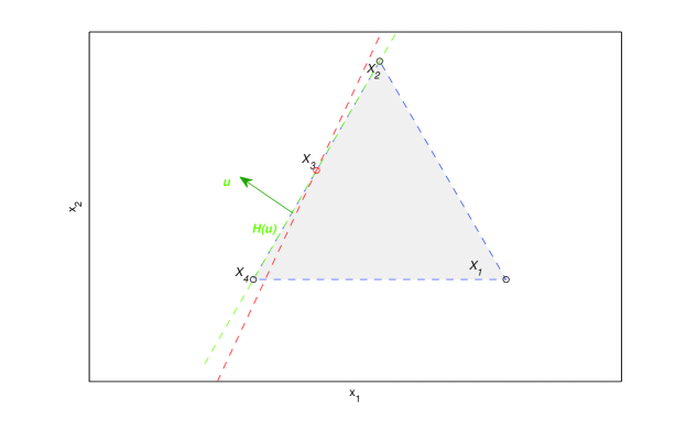
Figure 1: Shown is an example of the $\tau$-irrotatable halfspace. Observe that: (a) $\mathcal{H}(\textbf{u})$ cuts away no more than 1 sample point, i.e., $X_{1}$, and (b) $\partial\mathcal{H}(\textbf{\emph{u}})$ passes through at least $2\ (=d)$ sample points, i.e., $X_{2}$, $X_{3}$, $X_{4}$, and it is possible to make $\mathcal{H}(\textbf{\emph{u}})$ cutting away more than $\lceil 4\times 1/2\rceil-1=1$ sample points, i.e., $X_{1}$ and $X_{2}$, through deviating it by an arbitrary small scale around $X_{3}$. Hence, $\mathcal{H}(\textbf{\emph{u}})$ is $1/2$-irrotatable.

Remarkably, if a $\tau_{1}$-irrotatable halfspace cuts away strictly less than $\lceil n\tau_{1}\rceil-1$ sample points, it also should must be $\tau_{2}$-irrotatable for some $\tau_{2}<\tau_{1}$.

This $\tau$-irrotatable property is quite important for the following lemma, which further plays a key role in the proof of Lemma 4.

Lemma 3. Suppose $\mathcal{X}^{n}=\{X_{1},X_{2},\cdots,X_{n}\}\subset\mathcal{R}^{d}~{}(d\geq 2)$ is of affine dimension $d$. Then for $\forall\tau\in(0,\lambda^{*}]$, we have

$$\mathcal{D}_{\tau}(\mathcal{X}^{n})=\bigcap_{i=1}^{m_{\tau}}\mathcal{H}_{\tau}(\mu_{i}),$$

where $m_{\tau}$ denotes the number of all $\tau$-irrotatable halfspaces $\mathcal{H}_{\tau}(\mu_{i})$.

Proof. By (3), $\mathcal{D}_{\tau}(\mathcal{X}^{n})\subset\bigcap_{i=1}^{m_{\tau}}\mathcal{H}_{\tau}(\mu_{i})$ holds trivially. Hence, in the sequel we only prove: $\mathcal{D}_{\tau}(\mathcal{X}^{n})\supset\bigcap_{i=1}^{m_{\tau}}\mathcal{H}_{\tau}(\mu_{i})$.

If there $\exists\textbf{\emph{x}}_{0}\in\bigcap_{i=1}^{m_{\tau}}\mathcal{H}_{\tau}(\mu_{i})$ such that $\textbf{\emph{x}}_{0}\notin\mathcal{D}_{\tau}(\mathcal{X}^{n})$, i.e., $D(\textbf{\emph{x}}_{0},F_{n})<\tau$, we now show that this will lead to a contradiction. For simplicity, hereafter denote $\mathcal{V}_{n}(\tau)=\bigcap_{i=1}^{m_{\tau}}\mathcal{H}_{\tau}(\mu_{i})$.

Since $P_{n}(\cdot)$ takes values only on $\{0,1/n,2/n,\cdots,n/n\}$, there $\exists\textbf{\emph{u}}_{0}\in\mathcal{S}^{d-1}$ such that

$$P_{n}(\textbf{\emph{u}}_{0}^{\top}X\leq\textbf{\emph{u}}_{0}^{\top}\textbf{\emph{x}}_{0})=D(\textbf{\emph{x}}_{0},F_{n}).$$ (4)

Trivially, when $\mathcal{X}^{n}$ is of affine dimension $d$, we have: $\mathcal{V}_{n}(\tau)\subset\textbf{cov}(\mathcal{X}^{n})$ for $\forall\tau\in(0,\lambda^{*}]$, where $\textbf{cov}(\mathcal{X}^{n})$ denotes the convex hull of $\mathcal{X}^{n}$. Hence, for $\textbf{\emph{x}}_{0}\in\mathcal{V}_{n}(\tau)$ and $\textbf{\emph{u}}_{0}$ given in (4), there must exist an integer $k_{0}\in\{1,2,\cdots,n\lambda^{*}\}$ and a permutation $\pi_{0}:=(i_{1},i_{2},\cdots,i_{n})$ of $(1,2,\cdots,n)$ such that

$$\textbf{\emph{u}}_{0}^{\top}X_{i_{1}}\leq\textbf{\emph{u}}_{0}^{\top}X_{i_{2}}\leq\cdots\leq\textbf{\emph{u}}_{0}^{\top}X_{i_{k_{0}}}\leq\textbf{\emph{u}}_{0}^{\top}\textbf{\emph{x}}_{0}<\textbf{\emph{u}}_{0}^{\top}X_{i_{k_{0}+1}}\leq\cdots\leq\textbf{\emph{u}}_{0}^{\top}X_{i_{n}}.$$ (5)

Obviously, $k_{0}/n<\tau$ due to $D(\textbf{\emph{x}}_{0},F_{n})<\tau$, and hence $k_{0}\leq\lceil n\tau\rceil-1$.

Note that replacing $\textbf{\emph{u}}\in\mathcal{S}^{d-1}$ with $\textbf{\emph{u}}\in\mathcal{R}^{d}\setminus\{0\}$ does no harm to the definition of both $D(\textbf{\emph{x}},F_{n})$ and $\mathcal{D}_{\tau}(\mathcal{X}^{n})$ (Liu and Zuo, 2014). Hence, in the sequel we pretend that the constraint on u is $\textbf{\emph{u}}\in\mathcal{R}^{d}\setminus\{0\}$ instead.

Denote $\mathcal{C}(\pi_{0})=\{\textbf{\emph{v}}\in\mathcal{R}^{d}\setminus\{0\}:\textbf{\emph{v}}^{\top}X_{i_{t}}\leq\textbf{\emph{v}}^{\top}X_{i_{k_{0}+1}}\text{ for any }1\leq t\leq k_{0},\text{ and }\textbf{\emph{v}}^{\top}X_{i_{k_{0}+1}}\leq\textbf{\emph{v}}^{\top}X_{i_{s}}\text{ for any }k_{0}+2\leq s\leq n\}$. Obviously, $\textbf{\emph{u}}_{0}\in\mathcal{C}({\pi_{0}})$, and $\mathcal{C}(\pi_{0})$ is a convex cone.

Let $\mathcal{U}:=\{\nu_{j}\}_{j=1}^{m_{v}}=\{\textbf{\emph{z}}\in\mathcal{R}^{d}\setminus\{0\}:\|\textbf{\emph{z}}\|=1,~{}\textbf{\emph{z}}\text{ lies in a vertex of }\mathcal{C}({\pi_{0}})\}$ with $m_{v}$ being $\mathcal{U}$’s cardinal number. Clearly, $m_{v}<\infty$ and $\nu_{1},\nu_{2},\cdots,\nu_{m_{\tau}}$ are non-coplanar when $\mathcal{X}^{n}$ is of affine dimension $d$. By the construction of $\mathcal{C}({\pi_{0}})$, each $\nu\in\mathcal{U}$ determines a halfspace $\mathcal{H}(\nu)$ such that: (p1) $\nu$ is normal to $\partial\mathcal{H}(\nu)$ and points into the interior of $\mathcal{H}(\nu)$, (p2) $\mathcal{H}(\nu)$ cuts away at most $\lceil n\tau\rceil-1$ sample points, because $X_{i_{k_{0}+1}},X_{i_{k_{0}+2}},\cdots,X_{i_{n}}\in\mathcal{H}_{\nu}$, (p3) $\partial\mathcal{H}(\nu)$ contains at least $d$ sample points, which are of affine dimension $d-1$ due to $\nu$ is a vertex of $\mathcal{C}({\pi_{0}})$.

For $\mathcal{U}$, we claim that: there $\exists\textbf{\emph{v}}_{0}\in\mathcal{U}$ satisfying $\textbf{\emph{v}}_{0}^{\top}\textbf{\emph{x}}_{0}<\textbf{\emph{v}}_{0}^{\top}X_{i_{k_{0}+1}}$. If not, $\nu_{j}^{\top}\textbf{\emph{x}}_{0}\geq\nu_{j}^{\top}X_{i_{k_{0}+1}}$ for all $j=1,2,\cdots,m_{v}$. Hence,

$$\left(\sum_{j=1}^{m_{v}}\omega_{j}\nu_{j}\right)^{\top}\textbf{\emph{x}}_{0}\geq\left(\sum_{j=1}^{m_{v}}\omega_{j}\nu_{j}\right)^{\top}X_{i_{k_{0}+1}},$$

where $\sum_{j=1}^{m_{v}}\omega_{j}=1$ with $\omega_{j}\geq 0$ for all $j=1,2,\cdots,m_{v}$. This contradicts with (5) by noting that $\mathcal{C}(\pi_{0})$ is convex and $\textbf{\emph{u}}_{0}\in\mathcal{C}(\pi_{0})$.

However, $\textbf{\emph{v}}_{0}^{\top}\textbf{\emph{x}}_{0}<\textbf{\emph{v}}_{0}^{\top}X_{i_{k_{0}+1}}$ implies $\textbf{\emph{x}}_{0}\notin\mathcal{H}(\textbf{\emph{v}}_{0})$. We have:

1. $\mathcal{H}(\textbf{\emph{v}}_{0})$ satisfies (b) given in Page (b): By (p1)-(p3), $\mathcal{H}(\textbf{\emph{v}}_{0})$ is $\tau$-irrotatable, contradicting with the definition of $\mathcal{V}_{n}(\tau)$.

2. $\mathcal{H}(\textbf{\emph{v}}_{0})$ does not satisfy (b): Among all sample points contained by $\partial\mathcal{H}(\textbf{\emph{v}}_{0})$, there must exist $d-1$ points that determine a $(d-2)$-dimensional hyperplane, around which we can obtain a $\tau$-irrotatable halfspace through rotating $\mathcal{H}(\textbf{\emph{v}}_{0})$.

   (If not, there will be a contradiction: By (p2), there $\exists X_{j_{1}}$, $X_{j_{2}}$, $\cdots,X_{j_{d}}\in\partial\mathcal{H}(\textbf{\emph{v}}_{0})$, which are of affine dimension $d-1$. Denote $\mathbf{W}_{1},\mathbf{W}_{2},\cdots,\mathbf{W}_{d}$ respectively as ${d\choose d-1}$ hyperplanes that passing through all $(d-2)$-dimensional facets of the simplex formed by $X_{j_{1}},X_{j_{2}},\cdots,X_{j_{d}}$. Then similar to Part (II) of the proof of Theorem 1 in Liu et al. (2015a), it is easy to check that:

   for $\forall\textbf{\emph{y}}\in\mathcal{R}^{d}$, y can not simultaneously lie in all $\mathbf{W}_{1},\mathbf{W}_{2},\cdots,\mathbf{W}_{d}$.

   Without confusion, assume $\textbf{\emph{y}}\notin\mathbf{W}_{1}$ and $X_{j_{1}}\in\mathbf{W}_{1}$. Observe that no $\tau$-irrotatable halfspace is available through rotating $\mathcal{H}(\textbf{\emph{v}}_{0})$ around $\mathbf{W}_{1}$. Hence, for $\forall\delta>0$,

   $$\max\{nP_{n}(X\in\mathcal{H}_{\delta+}^{c}),~{}nP_{n}(X\in\mathcal{H}_{\delta-}^{c})\}<\lceil n\tau\rceil-1,$$ (6)

   where $\mathcal{H}_{\delta+}=\{\textbf{\emph{z}}\in\mathcal{R}^{d}:\textbf{\emph{u}}_{+}^{\top}\textbf{\emph{z}}\geq\textbf{\emph{u}}_{+}^{\top}X_{j_{1}}\}$, and $\mathcal{H}_{\delta-}=\{\textbf{\emph{z}}\in\mathcal{R}^{d}:\textbf{\emph{u}}_{-}^{\top}\textbf{\emph{z}}\geq\textbf{\emph{u}}_{-}^{\top}X_{j_{1}}\}$ with $\textbf{\emph{u}}_{+}=\textbf{\emph{v}}_{0}+\delta\textbf{\emph{u}}_{*}$ and $\textbf{\emph{u}}_{-}=\textbf{\emph{v}}_{0}-\delta\textbf{\emph{u}}_{*}$, where $\textbf{\emph{u}}_{*}\in\mathcal{S}^{d-1}$ is orthogonal to both $\textbf{\emph{v}}_{0}$ and $\mathbf{W}_{1}$. Since either $\textbf{\emph{y}}\in\mathcal{H}_{\delta+}^{c}$ or $\textbf{\emph{y}}\in\mathcal{H}_{\delta-}^{c}$ for $\forall\delta>0$, we obtain $D(\textbf{\emph{y}},F_{n})<(\lceil n\tau\rceil-1)/n\leq\tau$. This is impossible because $\mathcal{D}_{n}(\tau)$ is nonempty for $\forall\tau\in(0,\lambda^{*}]$.)

   Furthermore, it is easy to show that: if there is a $\tau$-irrotatable halfspace, say $\mathcal{H}_{1}$, obtained through rotating $\mathcal{H}(\textbf{\emph{v}}_{0})$ around one $(d-2)$-dimensional hyperplane clockwise (without confision), then there would be an another $\tau$-irrotatable halfspace, say $\mathcal{H}_{2}$, by rotating $\mathcal{H}(\textbf{\emph{v}}_{0})$ anti-clockwise. By noting $\mathcal{H}^{c}(\textbf{\emph{v}}_{0})\subset\mathcal{H}_{1}^{c}\cup\mathcal{H}_{2}^{c}$, we can obtain either $\textbf{\emph{x}}_{0}\in\mathcal{H}_{1}^{c}$ or $\textbf{\emph{x}}_{0}\in\mathcal{H}_{2}^{c}$, which contradicts with the definition of $\mathcal{V}_{n}(\tau)$.

Hence, there is no such $\textbf{\emph{x}}_{0}$ that $\textbf{\emph{x}}_{0}\in\mathcal{V}_{n}(\tau)$, but $\textbf{\emph{x}}_{0}\notin\mathcal{D}_{\tau}(\mathcal{X}^{n})$.

This completes the proof of this lemma. $\Box$

Remark 1. It may have long been known in the statistical community that Tukey’s sample depth regions may be polyhedral and have a finite number of facets. The detailed character of each facet of these regions is unknown, nevertheless. When $\mathcal{X}^{n}$ is in general position, Paindaveine and Šiman (2011) have shown that each hyperplane passing through a facet of $\mathcal{D}_{\tau}(\mathcal{X}^{n})$, for $\forall\tau\in(0,\lambda^{*}]$, contains exactly $d$ and cuts away exactly $\lceil n\tau\rceil-1$ sample points; see Lemma 4.1 in Page 201 of Paindaveine and Šiman (2011) for details. Lemma 3 generalizes their result by removing the ‘in general position’ assumption, and indicates that such hyperplanes contain at least $d$ and cuts away no more than $\lceil n\tau\rceil-1$ sample points.

To facilitate the understanding, we provide an illustrative example in Figure 2. In this example, there are $n=4$ observations, i.e., $X_{1},X_{2},X_{3},X_{4}$, where $X_{3}$ and $X_{4}$ take the same value. Clearly, they are not in general position and of affine dimension 2. Figures 2(a)-2(b) indicate that $\{X_{1},X_{3},X_{4}\}$ determines two $1/2$-irrotatable halfspaces, i.e., $\mathcal{H}_{1/2}(\textbf{\emph{u}}_{1})$ and $\mathcal{H}_{1/2}(\textbf{\emph{u}}_{2})$, satisfying $\mathcal{H}_{1/2}(\textbf{\emph{u}}_{1})\cap\mathcal{H}_{1/2}(\textbf{\emph{u}}_{2})=L_{1}$. Similarly, the intersection of the halfspaces determined by $\{X_{2},X_{3},X_{4}\}$ is $L_{2}$. Hence, the median region is $\{\textbf{\emph{x}}:\textbf{\emph{x}}=X_{3}\}$. From Figure 2(b) we can see that $\partial\mathcal{H}_{1/2}(\textbf{\emph{u}}_{2})$ contains $3\ (\neq 2)$ and $\mathcal{H}_{1/2}(\textbf{\emph{u}}_{2})$ cuts away $0\ (\neq 1)$ sample points, which obviously is not in agreement with the results of Paindaveine and Šiman (2011).

4 The limiting breakdown point of HM

In this section, we will derive the limit of the finite sample breakdown point of HM when the underlying distribution satisfies only the weak smooth condition (such a limit is also called asymptotic breakdown point in the literature, the latter notion is based on the maximum bias notion though, see Hampel(1968)). Since HM reduces to the ordinary univariate median for $d=1$, whose breakdown point robustness has been well studied, we focus only on the scenario of $d\geq 2$ in the sequel.

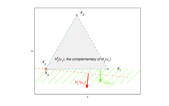
(a) Halfspace $\mathcal{H}_{1/2}(u_{1})$, which is $1/2$-irrotatable because $4P_{n}(X\in\mathcal{H}_{\tau}^{c}(u_{1}))\leq\lceil 4\tau\rceil-1$ but $4P_{n}(X\notin\mathcal{H}_{\tau}^{*}(u_{1}))=2>\lceil 4\tau\rceil-1$ for $\tau=1/2$.

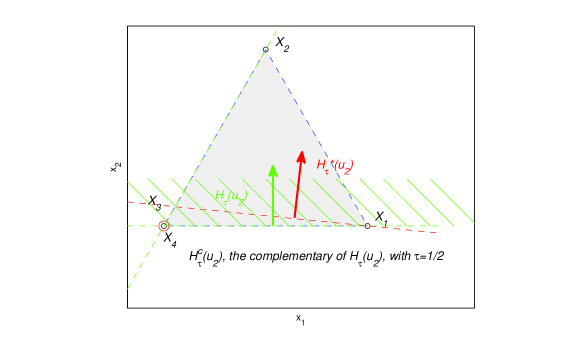
(b) Halfspace $\mathcal{H}_{1/2}(u_{2})$, which is similarly $1/2$-irrotatable because $4P_{n}(X\in\mathcal{H}_{\tau}^{c}(u_{2}))\leq\lceil 4\tau\rceil-1$ but $4P_{n}(X\notin\mathcal{H}_{\tau}^{*}(u_{2}))=2>\lceil 4\tau\rceil-1$ for $\tau=1/2$

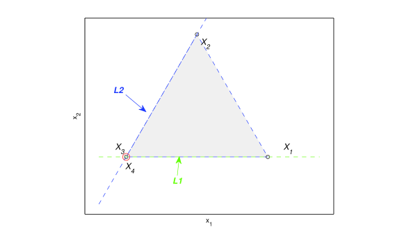
(c) The intersection of lines $L_{1}$ and $L_{2}$.

Figure 2: Shown are examples of the $\tau$-irrotatable halfspaces and related HM.

The key idea is to obtain simultaneously a lower and an upper bound of $\varepsilon(T^{*},\mathcal{X}^{n})$ for fixed $n$, and then prove that they tend to the same value as $n\rightarrow\infty$. When $\mathcal{X}^{n}$ is of affine dimension $d$, it is easy to obtain a lower bound, i.e., $\frac{\lambda^{*}}{1+\lambda^{*}}$, for $\varepsilon(T^{*},\mathcal{X}^{n})$ by using a similar strategy to Donoho and Gasko (1992) though. Finding a proper upper bound is not trivial, nevertheless.

To this end, we establish the following lemma, which provides a sharp upper bound with its limit coinciding with that of $\frac{\lambda^{*}}{1+\lambda^{*}}$ asymptotically. For simplicity, denoting by $\mathbb{A}_{\textbf{\emph{u}}}$ an arbitrary $d\times(d-1)$ matrix of unit vectors such that $(\textbf{\emph{u}}\,\vdots\,\mathbb{A}_{\textbf{\emph{u}}})$ constitutes an orthonormal basis of $\mathcal{R}^{d}$, we define the $\mathbb{A}_{\textbf{\emph{u}}}$-projections of $\mathcal{X}^{n}$ as $\mathbf{X}_{\textbf{\emph{u}}}^{n}=\{\mathbb{A}_{\textbf{\emph{u}}}^{\top}X_{1},\mathbb{A}_{\textbf{\emph{u}}}^{\top}X_{2},\cdots,\mathbb{A}_{\textbf{\emph{u}}}^{\top}X_{n}\}$ for $\forall\textbf{\emph{u}}\in\mathcal{S}^{d-1}$. Correspondingly, let $\hat{\theta}_{n}^{\textbf{\emph{u}}}=T^{*}(\mathbf{X}_{\textbf{\emph{u}}}^{n})$, $\lambda_{\textbf{\emph{u}}}^{*}=D(\hat{\theta}_{n}^{\textbf{\emph{u}}},F_{\textbf{\emph{u}}n})$, and $F_{\textbf{\emph{u}}n}$ to be the empirical distribution related to $\mathbf{X}_{\textbf{\emph{u}}}^{n}$.

Lemma 4. For a given data set $\mathcal{X}^{n}$ of affine dimension $d$, the finite sample breakdown point of Tukey’s halfspace median satisfies

$$\varepsilon(T^{*},\mathcal{X}^{n})\leq\frac{\inf_{{\textbf{\emph{u}}\in\mathcal{S}^{d-1}}}\lambda_{\textbf{\emph{u}}}^{*}}{1+\inf_{{\textbf{\emph{u}}\in\mathcal{S}^{d-1}}}\lambda_{\textbf{\emph{u}}}^{*}}.$$

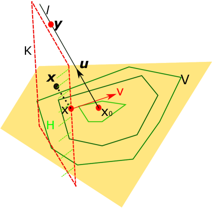
Figure 3: Shown is a 3-dimensional illustration. Once y’s are putted on $\ell$, all of their projections onto $\mathbf{V}$ are $\textbf{x}_{0}$. Hence, for any $\textbf{\emph{x}}\notin\ell$, its depth with respect to $\mathcal{X}^{n}\cup\mathcal{Y}^{m}$ would be no more than that of $\mathbf{x}$ with respect to the projections of $\mathcal{X}^{n}\cup\mathcal{Y}^{m}$, because all projections of the sample points contained by K would lie in $\mathbf{H}$. Here $\mathbf{H}$ denotes the optimal $(d-1)$-dimensional optimal halfspace of x, and $\mathbf{K}$ the $d$-dimensional halfspace whose projection is $\mathbf{H}$.

Since the whole proof of this lemma is very long, we present it in two parts. For $\forall\textbf{\emph{u}}\in\mathcal{S}^{d-1}$, in Part (I), we first project $\mathcal{X}^{n}$ onto a $(d-1)$-dimensional space $\textbf{V}_{d-1}^{\textbf{\emph{u}}}$ that is orthogonal to u, and then show that there $\exists\textbf{x}_{0}\in\textbf{V}_{d-1}^{\textbf{\emph{u}}}$, which can lie in the inner of the complementary of a $(d-1)$-dimensional optimal halfspace of $\forall\textbf{x}\in\textbf{V}_{d-1}^{\textbf{\emph{u}}}\setminus\{\textbf{x}_{0}\}$. Here by optimal halfspace of x we mean the halfspace realizing the depth at x with respect to $\mathbf{X}_{\textbf{\emph{u}}}^{n}$. Denote the line passing through $\mathbf{x}_{0}$ and parallel to u as $\ell_{\textbf{\emph{u}}}$. In Part (II), we will show that by putting $n\lambda_{\textbf{\emph{u}}}^{*}$ repetitions of $\textbf{\emph{y}}_{0}$ at any position on $\ell_{\textbf{\emph{u}}}$ but outside the convex hull of $\mathcal{X}^{n}$, i.e., $\ell_{\textbf{\emph{u}}}\setminus\textbf{cov}(\mathcal{X}^{n})$, it is possible to obtain that $\sup_{\textbf{\emph{x}}\in\textbf{cov}(\mathcal{X})}D(\textbf{\emph{x}},\mathcal{X}^{n}\cup\mathcal{Y}^{m})\leq n\lambda_{\textbf{\emph{u}}}^{*}$. Hence, $\inf_{\textbf{\emph{u}}\in\mathcal{S}^{d-1}}n\lambda_{\textbf{\emph{u}}}^{*}$ repetitions of $\textbf{\emph{y}}_{0}$ suffice for breaking down $T^{*}(\mathcal{X}^{n}\cup\mathcal{Y}^{m})$. See Figure 3 for a 3-dimensional illustration.

Proof of Lemma 4. Trivially, it is easy to check that, for $\forall\textbf{\emph{u}}\in\mathcal{S}^{d-1}$, $\mathbf{X}_{\textbf{\emph{u}}}^{n}$ is of affine dimension $d-1$ if $\mathcal{X}^{n}$ is of affine dimension $d$.

(I). In this part, we only prove that: When the affine dimension of $\mathcal{M}(\mathbf{X}_{\textbf{\emph{u}}}^{n})$ is nonzero for $d>2$, there $\exists\mathbf{x}_{0}\in\mathcal{M}(\mathbf{X}_{u}^{n})$ such that $\mathcal{U}_{\mathbf{x}}\cap\mathcal{H}_{\mathbf{x},\mathbf{x}_{0}}\neq\emptyset$ for $\forall\mathbf{x}\in\mathcal{M}(\mathbf{X}_{\textbf{\emph{u}}}^{n})\setminus\{\mathbf{x}_{0}\}$, where $\mathcal{U}_{\mathbf{x}}=\{\mathbf{v}\in\mathcal{S}^{d-2}:P_{n}(\mathbf{v}^{\top}(\mathbb{A}_{\textbf{\emph{u}}}^{\top}X)\leq\mathbf{v}^{\top}\mathbf{x})=D(\mathbf{x},F_{\textbf{\emph{u}}n})\}$, and $\mathcal{H}_{\mathbf{x},\mathbf{x}_{0}}=\{\mathbf{v}\in\mathcal{S}^{d-2}:\mathbf{v}^{\top}\mathbf{x}<\mathbf{v}^{\top}\mathbf{x}_{0}\}$. That is, $\mathbf{x}_{0}$ lies in the inner of the complementary of a $(d-1)$-dimensional optimal halfspace of $\forall\textbf{x}\in\mathcal{M}(\mathbf{X}_{\textbf{\emph{u}}}^{n})\setminus\{\textbf{x}_{0}\}$. The rest proof follows a similar fashion to Lemmas 2-3 of Liu et al. (2015b).

By Lemma 3, $\mathcal{M}(\mathbf{X}_{\textbf{\emph{u}}}^{n})$ is polyhedral. Similar to Theorem 2 of Liu et al. (2015a), we can obtain that, if there is a sample point $X_{i}$ such that $\mathbb{A}_{\textbf{\emph{u}}}^{\top}X_{i}\in\mathcal{M}(\mathbf{X}_{\textbf{\emph{u}}}^{n})$, then $\mathbb{A}_{\textbf{\emph{u}}}^{\top}X_{i}$ should be a vertex of $\mathcal{M}(\mathbf{X}_{\textbf{\emph{u}}}^{n})$ based on the representation of $\mathcal{M}(\mathbf{X}_{\textbf{\emph{u}}}^{n})$ obtained in Lemma 3. Let $\mathbf{V}_{\textbf{\emph{u}}}$ be the set of vertexes of $\mathcal{M}(\mathbf{X}_{\textbf{\emph{u}}}^{n})$ such that, for $\forall\textbf{y}\in\mathbf{V}_{\textbf{\emph{u}}}$, there is an optimal halfspace $\mathbf{H}_{\textbf{y}}$ of y satisfying $\mathbf{H}_{\textbf{y}}\cap\mathcal{M}(\mathbf{X}_{\textbf{\emph{u}}}^{n})=\{\textbf{y}\}$. Trivially, $\mathbb{A}_{\textbf{\emph{u}}}^{\top}X_{i}\in\mathbf{V}_{\textbf{\emph{u}}}$ if $\mathbb{A}_{\textbf{\emph{u}}}^{\top}X_{i}\in\mathcal{M}(\mathbf{X}_{\textbf{\emph{u}}}^{n})$.

If there is point in $\mathbf{V}_{\textbf{\emph{u}}}$ that can sever as $\mathbf{x}_{0}$, then this statement holds already. Otherwise, find a candidate point $\textbf{z}_{0}$ by using the following iterative procedure and then show that $\textbf{z}_{0}$ can be used as $\textbf{x}_{0}$. For simplicity, hereafter denote $\mathcal{A}_{\mathbf{z}}=\{\mathbf{x}\in\mathcal{R}^{d-1}:\mathcal{U}_{\mathbf{x}}\cap\mathcal{H}_{\mathbf{x},\mathbf{z}}\neq\emptyset\}$ and $\mathcal{B}_{\mathbf{z}}=\{\mathbf{x}\in\mathcal{R}^{d-1}:\mathcal{U}_{\mathbf{x}}\cap\mathcal{H}_{\mathbf{x},\mathbf{z}}=\emptyset\}$ for $\forall\mathbf{z}\in\mathcal{M}(\mathbf{X}_{u}^{n})$. Obviously, $\mathcal{A}_{\mathbf{z}}\cup\mathcal{B}_{\mathbf{z}}=\mathcal{R}^{d-1}$, $\mathcal{A}_{\mathbf{z}}\cap\mathcal{B}_{\mathbf{z}}=\emptyset$, $\mathbf{z}\in\mathcal{B}_{\mathbf{z}}$, and $\mathcal{B}_{\mathbf{z}}\subset\mathcal{M}(\mathbf{X}_{\textbf{\emph{u}}}^{n})$.

Let $\mathbf{z}_{1}=T^{*}(\mathbf{X}_{\textbf{\emph{u}}}^{n})$. Clearly, $\mathbf{V}_{\textbf{\emph{u}}}\cap\mathcal{B}_{\mathbf{z}_{1}}=\emptyset$. (In fact, $\mathbf{V}_{\textbf{\emph{u}}}\cap\mathcal{B}_{\mathbf{z}}=\emptyset$ for any $\mathbf{z}\in\mathcal{M}(\mathbf{X}_{\textbf{\emph{u}}}^{n})\setminus\mathbf{V}_{\textbf{\emph{u}}}$.) If $\mathcal{B}_{\mathbf{z}_{1}}=\{\textbf{z}_{1}\}$, let $\mathbf{x}_{0}=\mathbf{z}_{0}$ and this statement is already true. Otherwise, similar to Lemma 2 of Liu et al. (2015b), for $\forall\mathbf{x}\in\mathcal{B}_{\mathbf{z}_{1}}\setminus\{\mathbf{z}_{1}\}$, we obtain: (o1) $\mathbf{u}^{\top}\mathbf{x}\geq\mathbf{u}^{\top}\mathbf{z}_{1}$ for $\forall\mathbf{u}\in\mathcal{U}_{\mathbf{z}_{1}}$, (o2) $\mathcal{U}_{\mathbf{x}}\subset\mathcal{U}_{\mathbf{z}_{1}}$, and (o3) $\mathcal{B}_{\mathbf{x}}\subset\mathcal{B}_{\mathbf{z}_{1}}\setminus\{\mathbf{z}_{1}\}$.

Denote

$$g(\mathbf{z}_{1})=\sup_{\mathbf{v}\in\mathcal{U}_{\mathbf{z}_{1}},\mathbf{x}\in\mathcal{B}_{\mathbf{z}_{1}\setminus\{\mathbf{z}_{1}\}}}\mathbf{v}^{\top}(\mathbf{x}-\mathbf{z}_{1}).$$

Clearly, $g(\mathbf{z}_{1})>0$ by (o1)-(o3). Along the same line of Liu et al. (2015b), we can find a series $\{\mathbf{z}_{i}\}_{i=1}^{\infty}\subset\mathcal{M}(\mathbf{X}_{u}^{n})$, if there is no $m>1$ such that $\mathcal{B}_{\mathbf{z}_{m}}=\{\mathbf{z}_{m}\}$, satisfying that: $\{\mathbf{z}_{i}\}_{i=1}^{\infty}$ contains a convergent subsequence $\{\mathbf{z}_{i_{k}}\}_{k=1}^{\infty}$ with $\lim\limits_{k\rightarrow\infty}\mathbf{z}_{i_{k}}=\mathbf{z}_{0}$ and $\lim\limits_{k\rightarrow\infty}g(\mathbf{z}_{i_{k}-1})=0$. Trivially, $\mathbf{z}_{0}\in\mathcal{M}(\mathbf{X}_{\textbf{\emph{u}}}^{n})\setminus\mathbf{V}_{\textbf{\emph{u}}}$. (If not, it is easy to obtain a contradiction.)

Now we proceed to prove $\mathcal{B}_{\mathbf{z}_{0}}=\{\mathbf{z}_{0}\}$. First, we show

(F1):  $\mathbf{z}_{0}\in\mathcal{B}_{\mathbf{z}_{j-1}}\setminus\{\mathbf{z}_{j-1}\}$ for $\forall j\in\{i_{k}\}_{k=1}^{\infty}$.

If not, there must $\exists\tilde{\mathbf{u}}\in\mathcal{U}_{\mathbf{z}_{0}}$ satisfying $\tilde{\mathbf{u}}^{\top}\mathbf{z}_{0}<\tilde{\mathbf{u}}^{\top}\mathbf{z}_{j-1}$. For this $\tilde{\mathbf{u}}\in\mathcal{U}_{\mathbf{z}_{0}}$, let $(i_{1}^{\prime},i_{2}^{\prime},\cdots,i_{n}^{\prime})$ be the permutation of $(1,2,\cdots,n)$ such that: (a) $\tilde{\mathbf{u}}^{\top}(\mathbb{A}_{\textbf{\emph{u}}}^{\top}X_{i_{s}^{\prime}})\leq\tilde{\mathbf{u}}^{\top}\mathbf{z}_{0}$ for $1\leq s\leq k^{*}$, and (b) $\tilde{\mathbf{u}}^{\top}(\mathbb{A}_{\textbf{\emph{u}}}^{\top}X_{i_{t}^{\prime}})>\tilde{\mathbf{u}}^{\top}\mathbf{z}_{0}$ for $k^{*}+1\leq t\leq n$, where $k^{*}=n\lambda_{\textbf{\emph{u}}}^{*}$. Denote

$$\varepsilon_{0}=\frac{1}{2}\min\left\{\min_{k^{*}+1\leq t\leq n}\tilde{\mathbf{u}}^{\top}((\mathbb{A}_{\textbf{\emph{u}}}^{\top}X_{i_{t}^{\prime}})-\mathbf{z}_{0}),~{}\tilde{\mathbf{u}}^{\top}(\mathbf{z}_{j-1}-\mathbf{z}_{0})\right\}.$$

Since $\{\mathbf{z}_{i_{k}}\}_{k=1}^{\infty}$ is convergent, there must $\exists j^{*}\in\{i_{k}\}_{k=1}^{\infty}$ with $j^{*}>j$ such that $\|\mathbf{z}_{j^{*}}-\mathbf{z}_{0}\|<\varepsilon_{0}$. This, together with $|\tilde{\mathbf{u}}^{\top}(\mathbf{z}_{j^{*}}-\mathbf{z}_{0})|\leq\|\mathbf{z}_{j^{*}}-\mathbf{z}_{0}\|$, leads to $\tilde{\mathbf{u}}^{\top}\mathbf{z}_{j^{*}}<\tilde{\mathbf{u}}^{\top}(\mathbb{A}_{u}^{\top}X_{i_{t}^{\prime}})$ for $k^{*}+1\leq t\leq n$, which further implies $P_{n}(\tilde{\mathbf{u}}^{\top}(\mathbb{A}_{u}^{\top}X)\leq\tilde{\mathbf{u}}^{\top}\mathbf{z}_{j^{*}})\leq\lambda_{\textbf{\emph{u}}}^{*}$. Next, by noting $\lambda_{\textbf{\emph{u}}}^{*}=D(\mathbf{z}_{j^{*}},F_{n}^{u})\leq P_{n}(\tilde{\mathbf{u}}^{\top}(\mathbb{A}_{u}^{\top}X)\leq\tilde{\mathbf{u}}^{\top}\mathbf{z}_{j^{*}})$, we obtain $\tilde{\mathbf{u}}\in\mathcal{U}_{\mathbf{z}_{j^{*}}}\subset\mathcal{U}_{\mathbf{z}_{j-1}}$. On the other hand, for $\varepsilon_{0}$, a similar derivation leads to $\tilde{\mathbf{u}}^{\top}\mathbf{z}_{j^{*}}<\tilde{\mathbf{u}}^{\top}\mathbf{z}_{j-1}$. This contradicts with $\mathbf{z}_{j^{*}}\in\mathcal{B}_{\mathbf{z}_{j-1}}$ when $j^{*}>j$ by (o1)-(o2). Then, based on $\lim\limits_{k\rightarrow\infty}g(\mathbf{z}_{i_{k}-1})=0$ and (F1), we can obtain $\mathcal{B}_{\mathbf{z}_{0}}\setminus\{\mathbf{z}_{0}\}=\emptyset$ similar to Lemma 3 of Liu et al. (2015b). Hence, we may let $\mathbf{x}_{0}=\mathbf{z}_{0}$.

(II). By denoting $\ell_{\textbf{\emph{u}}}=\{\textbf{\emph{z}}\in\mathcal{R}^{d}:\textbf{\emph{z}}=\mathbb{A}_{\textbf{\emph{u}}}\mathbf{x}_{0}+\gamma\textbf{\emph{u}},~{}\forall\gamma\in\mathcal{R}^{1}\}$ and using a similar method to the first proof part of Theorem 1 in Liu et al. (2015b), we can obtain that, for an any given $\textbf{\emph{y}}_{0}\in\textbf{cov}(\mathcal{X}^{n})\setminus\ell_{\textbf{\emph{u}}}$, it holds $\sup_{\textbf{\emph{x}}\in\textbf{cov}(\mathcal{X}^{n})}D(\textbf{\emph{x}},F_{n+m})\leq\frac{n\lambda_{\textbf{\emph{u}}}^{*}}{n+m}$, where $F_{n+m}$ denotes the empirical distribution related to $\mathcal{X}^{n}\cup\mathcal{Y}^{m}$, and $\mathcal{Y}^{m}$ contains $m$ repetitions of $\textbf{\emph{y}}_{0}$.

Note that u is any given, and $D(\textbf{\emph{y}}_{0},F_{n+m})=\frac{m}{n+m}\geq\frac{n\lambda_{\textbf{\emph{u}}}^{*}}{n+m}$ when $m\leq n\lambda_{\textbf{\emph{u}}}^{*}$. Hence

$$\varepsilon(T^{*},\mathcal{X}^{n})\leq\frac{\inf_{{\textbf{\emph{u}}\in\mathcal{S}^{d-1}}}n\lambda_{\textbf{\emph{u}}}^{*}}{n+\inf_{{\textbf{\emph{u}}\in\mathcal{S}^{d-1}}}n\lambda_{\textbf{\emph{u}}}^{*}}=\frac{\inf_{{\textbf{\emph{u}}\in\mathcal{S}^{d-1}}}\lambda_{\textbf{\emph{u}}}^{*}}{1+\inf_{{\textbf{\emph{u}}\in\mathcal{S}^{d-1}}}\lambda_{\textbf{\emph{u}}}^{*}}.$$

This completes the proof. $\Box$

Observe that the upper bound given in Lemma 4 involves the $\mathbb{A}_{\textbf{\emph{u}}}$-projections. A nature problem arises: whether the $\mathbb{A}_{\textbf{\emph{u}}}$-projection of $X$ is still halfspace symmetrically distributed? The following lemma provides a positive answer to this question.

Lemma 5. Suppose $X$ is halfspace symmetrical about $\theta_{0}\in\mathcal{R}^{d}$ ($d\geq 2$). Then for $\forall\textbf{\emph{u}}\in\mathcal{S}^{d-1}$, $\mathbb{A}_{\textbf{\emph{u}}}^{\top}X$ is halfspace symmetrical about $\mathbb{A}_{\textbf{\emph{u}}}^{\top}\theta_{0}\in\mathcal{R}^{d-1}$.

Proof. For $\forall\mathbf{v}\in\mathcal{S}^{d-2}$, the fact $(\mathbb{A}_{\textbf{\emph{u}}}\mathbf{v})^{\top}(\mathbb{A}_{\textbf{\emph{u}}}\mathbf{v})=\mathbf{v}^{\top}(\mathbb{A}_{\textbf{\emph{u}}}^{\top}\mathbb{A}_{\textbf{\emph{u}}})\mathbf{v}=1$ implies $\mathbb{A}_{\textbf{\emph{u}}}\mathbf{v}\in\mathcal{S}^{d-1}$. Note that

$$P\left(\mathbf{v}^{\top}(\mathbb{A}_{\textbf{\emph{u}}}^{\top}X)\geq\mathbf{v}^{\top}(\mathbb{A}_{\textbf{\emph{u}}}^{\top}\theta_{0})\right)=P\left((\mathbb{A}_{\textbf{\emph{u}}}\mathbf{v})^{\top}X\geq(\mathbb{A}_{\textbf{\emph{u}}}\mathbf{v})^{\top}\theta_{0}\right)\geq\frac{1}{2}.$$

This completes the proof of this lemma.

Lemma 5 in fact obtains the population version, i.e., $D(\mathbb{A}_{\textbf{\emph{u}}}^{\top}\theta_{0},F_{\textbf{\emph{u}}})$, of $D(\hat{\theta}_{n}^{\textbf{\emph{u}}},F_{\textbf{\emph{u}}n})$ for $\forall\textbf{\emph{u}}\in\mathcal{S}^{d-1}$, where $F_{\textbf{\emph{u}}}$ denotes the distribution of $\mathbb{A}_{\textbf{\emph{u}}}^{\top}X$.

we now are in the position to prove the following theorem.

Theorem 1. Suppose that (C1) $\{X_{1},X_{2},\cdots,X_{n}\}\stackrel{{\scriptstyle\text{i.i.d.}}}{{\sim}}F$ is of affine dimension $d$, (C2) $F$ is halfspace symmetric about point $\theta_{0}$, and (C3) $F$ is smooth at point $\theta_{0}$. Then we have $\varepsilon(T^{*},\mathcal{X}^{n})\stackrel{{\scriptstyle\text{a.s.}}}{{\longrightarrow}}\frac{1}{3},\quad\text{as }n\rightarrow+\infty,$ where $\stackrel{{\scriptstyle\text{a.s.}}}{{\longrightarrow}}$ denotes the “almost sure convergence”.

Proof. Observe that

$$|D(\hat{\theta}_{n},F_{n})-D(\theta_{0},F)|\leq\underbrace{\sup_{\textbf{\emph{x}}\in\mathcal{R}^{d}}|D(\textbf{\emph{x}},F_{n})-D(\textbf{\emph{x}},F)|}_{\textbf{E1}}+\underbrace{|D(\hat{\theta}_{n},F)-D(\theta_{0},F)|}_{\textbf{E2}}.$$

Under Condition (C1), a direct use of Remark 2.5 in Page 1465 of Zuo (2003) leads to that

$$\sup_{\textbf{\emph{x}}\in\mathcal{R}^{d}}\left|D(\textbf{\emph{x}},F_{n})-D(\textbf{\emph{x}},F)\right|\stackrel{{\scriptstyle\text{a.s.}}}{{\longrightarrow}}0,\quad\text{as }n\rightarrow+\infty,$$ (7)

holds with no restriction on $F$. Hence, $\textbf{E1}\stackrel{{\scriptstyle\text{a.s.}}}{{\longrightarrow}}0$.

For E2, from Lemma 2, we have that $D(\textbf{\emph{x}},F)$ is continuous at $\theta_{0}$ under Condition (C3). On the other hand, since $D(\theta_{0},F)\geq 1/2>0$ under Condition (C2), an application of Lemma A.3 of Zuo (2003) leads to $\hat{\theta}_{n}\stackrel{{\scriptstyle\text{a.s.}}}{{\longrightarrow}}\theta_{0}$. These two facts together imply $\textbf{E2}\stackrel{{\scriptstyle\text{a.s.}}}{{\longrightarrow}}0$.

Based on $\textbf{E1}\stackrel{{\scriptstyle\text{a.s.}}}{{\longrightarrow}}0$ and $\textbf{E2}\stackrel{{\scriptstyle\text{a.s.}}}{{\longrightarrow}}0$, we in fact obtain

$$D(\hat{\theta}_{n},F_{n})\stackrel{{\scriptstyle\text{a.s.}}}{{\longrightarrow}}D(\theta_{0},F),\quad\forall\textbf{\emph{u}}\in\mathcal{S}^{d-1}.$$ (8)

Relying on this and the lower bound $\frac{\lambda^{*}}{1+\lambda^{*}}$, it is easy to show that

$$\varepsilon(T^{*},\mathcal{X}^{n})\geq\frac{D(\theta_{0},F)}{1+D(\theta_{0},F)},\quad\text{almost surely.}$$

By Lemma 5, $F_{\textbf{\emph{u}}}$ is also halfspace symmetrical and smooth at $\mathbb{A}_{\textbf{\emph{u}}}^{\top}\theta_{0}$ for $\forall\textbf{\emph{u}}\in\mathcal{S}^{d-1}$. Hence, a similar proof to (8) leads to

$$D(\hat{\theta}_{n}^{\textbf{\emph{u}}},F_{\textbf{\emph{u}}n})\stackrel{{\scriptstyle\text{a.s.}}}{{\longrightarrow}}D(\mathbb{A}_{\textbf{\emph{u}}}^{\top}\theta_{0},F_{\textbf{\emph{u}}}),\quad\text{as }n\rightarrow\infty.$$

This, together with Lemma 4, and the theory of empirical processes (Pollard, 1984), leads to

$$\varepsilon(T^{*},\mathcal{X}^{n})\leq\frac{\inf_{{\textbf{\emph{u}}\in\mathcal{S}^{d-1}}}D(\mathbb{A}_{\textbf{\emph{u}}}^{\top}\theta_{0},F_{\textbf{\emph{u}}})}{1+\inf_{{\textbf{\emph{u}}\in\mathcal{S}^{d-1}}}D(\mathbb{A}_{\textbf{\emph{u}}}^{\top}\theta_{0},F_{\textbf{\emph{u}}})},\quad\text{almost surely.}$$

Next, by

$$D(\mathbb{A}_{\textbf{\emph{u}}}^{\top}\theta_{0},F_{\textbf{\emph{u}}}) = \inf_{\mathbf{v}\in\mathcal{S}^{d-2}}P\left(\mathbf{v}^{\top}(\mathbb{A}_{\textbf{\emph{u}}}^{\top}X)\leq\mathbf{v}^{\top}(\mathbb{A}_{\textbf{\emph{u}}}^{\top}\theta_{0})\right)$$

$$= \inf_{\bar{\textbf{\emph{u}}}\in\mathcal{S}^{d-1},~{}\bar{\textbf{\emph{u}}}\bot\textbf{\emph{u}}}P(\bar{\textbf{\emph{u}}}^{\top}X\leq\bar{\textbf{\emph{u}}}^{\top}\theta_{0}),$$

where $\bar{\textbf{\emph{u}}}=\mathbb{A}_{\textbf{\emph{u}}}\mathbf{v}$, we obtain

$$\inf_{\textbf{\emph{u}}\in\mathcal{S}^{d-1}}D(\mathbb{A}_{\textbf{\emph{u}}}^{\top}\theta_{0},F_{\textbf{\emph{u}}}) = \inf_{\textbf{\emph{u}}\in\mathcal{S}^{d-1}}\left\{\inf_{\bar{\textbf{\emph{u}}}\in\mathcal{S}^{d-1},\bar{\textbf{\emph{u}}}\bot\textbf{\emph{u}}}P(\bar{\textbf{\emph{u}}}^{\top}X\leq\bar{\textbf{\emph{u}}}^{\top}\theta_{0})\right\}$$

$$= \inf_{\textbf{\emph{u}}\in\mathcal{S}^{d-1}}P(\textbf{\emph{u}}^{\top}X\leq\textbf{\emph{u}}^{\top}\theta_{0})$$

$$= D(\theta_{0},F).$$

This proves $\varepsilon(T^{*},\mathcal{X}^{n})\stackrel{{\scriptstyle\text{a.s.}}}{{\longrightarrow}}\frac{D(\theta_{0},F)}{1+D(\theta_{0},F)}=1/3$, because $D(\theta_{0},F)=\frac{1}{2}$ under Conditions (C2)-(C3). This completes the proof of this theorem. $\Box$

Remark 2   It is worth noting that, both halfspace symmetry and weak smooth condition assumptions in this paper can not be further relaxed if one wants to obtain exactly the limiting breakdown point of HM. The former is the weakest assumotion to guarantee to have a unique center. The latter is equivalent to the continuity of $D(\textbf{\emph{x}},F)$ at $\theta_{0}$, which is necessary for deriving the limit for both the lower and upper bound, while the upper bound given in Lemma 4 could not be further improved for fixed $n$.

5 Concluding remarks

In this paper, we consider the limit of the finite sample breakdown point of HM under weaker assumption on underlying distribution and data set. Under such assumptions, the random observations may not be ‘in general position’. This causes additional inconvenience to the derivation of the limiting result compared to the scenario of $\mathcal{X}^{n}$ being in general position. During our investigation, relationships between various smooth conditions have been established and the representation of the Tukey depth and median regions has also been obtained without imposing the ‘in general position’ assumption.

Tukey halfspace depth idea has been extended beyond the location setting to many other settings (e.g., regression, functional data, etc.). We anticipate that our results here could also be extended to those settings.

References

- Adrover and Yohai (2002) Adrover, J., Yohai, V., 2002. Projection estimates of multivariate location. Annals of statistics, 1760-1781.
- Chen (1995) Chen, Z., 1995. Robustness of the half-space median. Journal of statistical planning and inference, 46(2), 175-181.
- Chen and Tyler (2002) Chen, Z., Tyler, D.E., 2002. The influence function and maximum bias of Tukey’s median. Ann. Statist. 30, 1737-1759.
- Donoho (1982) Donoho, D.L., 1982. Breakdown properties of multivariate location estimators. Ph.D. Qualifying Paper. Dept. Statistics, Harvard University.
- Donoho and Gasko (1992) Donoho, D.L., Gasko, M., 1992. Breakdown properties of location estimates based on halfspace depth and projected outlyingness. Ann. Statist. 20, 1808-1827.
- Donoho and Huber (1983) Donoho, D.L., Huber, P.J., 1983. The notion of breakdown point. In: Bickel, P.J., Doksum, K.A., Hodges Jr., J.L. (Eds.), A Festschrift foe Erich L. Lehmann. Wadsworth, Belmont, CA, pp. 157-184.
- Hampel, F.R. (1968) Hampel, F.R. (1968). Contributions to the theory of robust estimation, Ph.D. Thesis, University of California, Berkeley.
- Kong and Zuo (2010) Kong, L., Zuo, Y. 2010. Smooth depth contours characterize the underlying distribution. J. Multivariate Anal., 101, 2222-2226.
- Kong and Mizera (2012) Kong, L., Mizera, I., 2012. Quantile tomography: Using quantiles with multivariate data. Statist. Sinica, 22, 1589-1610.
- Liu (1988) Liu, R. Y., 1988. On a notion of simplicial depth. Proc. Natl. Acad. Sci. USA. 85, 1732-1734.
- Liu (1990) Liu, R. Y., 1990. On a notion of data depth based on random simplices. Ann. Statist. 18, 191-219.
- Liu et al. (2013) Liu, X.H., Zuo, Y.J., Wang, Z.Z., 2013. Exactly computing bivariate projection depth median and contours. Comput. Statist. Data Anal. 60, 1-11.
- Liu et al. (2015a) Liu, X.H., Luo, S.H., Zuo, Y.J., 2015a. Some results on the computing of Tukey’s halfspace median. arXiv:1604.05927, Mimeo.
- Liu and Zuo (2014) Liu, X., Zuo, Y., 2014. Computing halfspace depth and regression depth. Communications in Statistics-Simulation and Computation, 43, 969-985.
- Liu et al. (2015b) Liu, X., Zuo, Y., Wang, Q., 2015b. Finite sample breakdown point of Tukey’s halfsapce median. Preprint on arXiv. Mimeo.
- Mosler et al. (2009) Mosler, K., Lange, T., Bazovkin, P., 2009. Computing zonoid trimmed regions of dimension . Comput. Statist. Data Anal. 53, 2500-2510.
- Paindaveine and Šiman (2011) Paindaveine, D., Šiman, M., 2011. On directional multiple-output quantile regression. J. Multivariate Anal. 102, 193-392.
- Pollard (1984) Pollard, D., 1984. Convergence of stochastic processes. Springer, New York.
- Tukey (1975) Tukey, J.W., 1975. Mathematics and the picturing of data. In Proceedings of the International Congress of Mathematicians, 523-531. Cana. Math. Congress, Montreal.
- Zuo (2001) Zuo, Y., 2001. Some quantitative relationships between two types of finite sample breakdown point. Stat. Probab. Lett. 51, 369-375.
- Zuo (2003) Zuo, Y.J., 2003. Projection based depth functions and associated medians. Ann. Statist. 31, 1460-1490.
- Zuo and Serfling (2000) Zuo, Y.J., Serfling, R., 2000. On the performance of some robust nonparametric location measures relative to a general notion of multivariate symmetry. Journal of Statistical Planning and Inference, 84(1), 55-79.