On the characterization of minimal surfaces with finite total curvature in $\operatorname{\mathbb{H}^{2}\times\mathbb{R}}$ and $\widetilde{\rm PSL}_{2}(\operatorname{\mathbb{R}})$

Abstract

It is known that a complete immersed minimal surface with finite total curvature in $\mathbb{H}^{2}\times\mathbb{R}$ is proper, has finite topology and each one of its ends is asymptotic to a geodesic polygon at infinity (Hauswirth and Rosenberg, 2006; Hauswirth, Nelli, Sa Earp and Toubiana, 2015). In this paper we prove that these three properties characterize complete immersed minimal surfaces with finite total curvature in $\mathbb{H}^{2}\times\mathbb{R}$. As corollaries of this theorem we obtain characterizations for minimal Scherk-type graphs and horizontal catenoids in $\mathbb{H}^{2}\times\mathbb{R}$. We also prove that if a properly immersed minimal surface in $\widetilde{\rm PSL}_{2}(\mathbb{R},\tau)$ has finite topology and each one of its ends is asymptotic to a geodesic polygon at infinity, then it must have finite total curvature.

1 Introduction

The theory of finite total curvature minimal surfaces in $\operatorname{\mathbb{H}^{2}\times\mathbb{R}}$ has been introduced by Collin and Rosenberg [5]. They remarked by Fatou’s convergence theorem in Gauss-Bonnet formula that complete minimal graphs over ideal polygonal domain of $\operatorname{\mathbb{H}^{2}}$ with a finite number of vertices (called Scherk-type graphs) have finite total curvature in $\operatorname{\mathbb{H}^{2}\times\mathbb{R}}$. Together with the vertical geodesic planes these were the first examples appearing in the theory. Later, Hauswirth and Rosenberg [13] proved that the total curvature of these surfaces is a multiple of $2Ê\pi$. They also began to describe their asymptotic geometric behavior at infinity and this description has been later completed by Hauswirth, Nelli, Sa Earp and Toubiana [12]. They proved that any complete minimal surface with finite total curvature in $\operatorname{\mathbb{H}^{2}\times\mathbb{R}}$ is proper, has finite topology and each one of its ends is asymptotic to an admissible polygon at infinity (see Definition 1 below).

The asymptotic boundary $\partial_{\infty}\mathbb{H}^{2}$ of $\mathbb{H}^{2}$ can be identified with the unit circle. There are different notions of asymptotic boundary $\partial_{\infty}(\operatorname{\mathbb{H}^{2}\times\mathbb{R}})$ of $\operatorname{\mathbb{H}^{2}\times\mathbb{R}}$. In this paper we use the product compactification obtained as the product of the compactications of each one of the factors. This is, we consider the following model for $\partial_{\infty}(\operatorname{\mathbb{H}^{2}\times\mathbb{R}})$: $((\partial_{\infty}\operatorname{\mathbb{H}^{2}})\times[-1,+1])\cup(\operatorname{\mathbb{H}^{2}}\times\{\pm 1\}),$ where we represent the second factor $\mathbb{R}$ by some homeomorphism $\phi:\mathbb{R}\to(-1,1)$.

We say that $p\in\partial_{\infty}(\operatorname{\mathbb{H}^{2}\times\mathbb{R}})$ is in the asymptotic boundary of a minimal surface ${\cal M}$ if there is a diverging sequence of points $p_{n}\in{\cal M}$ such that $p_{n}$ converges to $p$ in the compactification. This means that if $p_{n}=(z_{n},t_{n})\in{\cal M}$ and $p=(a,h)\in\partial_{\infty}(\operatorname{\mathbb{H}^{2}\times\mathbb{R}})$, then $z_{n}\to a$ in the compactification of $\operatorname{\mathbb{H}^{2}}$ and $\phi(t_{n})\to h$ in $[-1,1]$.

Given a vertical geodesic plane ${\cal M}=\alpha\times\mathbb{R}$, where $\alpha$ is a horizontal geodesic with two endpoints $a_{1},a_{2}\in\partial_{\infty}\operatorname{\mathbb{H}^{2}}$, we have $\partial_{\infty}{\cal M}=(\alpha\times\{\pm 1\})\cup(\{a_{1},a_{2}\}\times[-1,1])$. This boundary can be viewed as a quadrilateral curve at infinity. We generalize this construction by the following definition.

Definition 1 (Admissible polygon at infinity).

We call polygon at infinity to any (connected, closed) polygon in $\partial_{\infty}(\operatorname{\mathbb{H}^{2}\times\mathbb{R}})$ composed of a finite number of geodesics. We say that a polygon at infinity ${\cal P}$ is admissible if there exists an even number of geodesics $\alpha_{1},\beta_{1},...,\alpha_{k},\beta_{k}\subset\operatorname{\mathbb{H}^{2}}$ such that $\mathcal{P}$ is the union of the geodesics at infinity $\alpha_{i}\times\{+1\}$ and $\beta_{i}\times\{-1\}$, with $i=1,...,k$, together with the corresponding vertical straight lines $L_{i}=\{a_{i}\}\times[-1,1]$, $a_{i}\in\partial_{\infty}\operatorname{\mathbb{H}^{2}}$, joining their endpoints (see Figure 1).

Definition 2 (Embedded Admissible polygon).

We say that an admissible polygon ${\cal P}$ is embedded if there exists a one-to-one correspondence from $\operatorname{\mathbb{S}}^{1}$ to ${\cal P}$.

We observe that the projection over $\operatorname{\mathbb{H}^{2}}$ of an embedded admissible polygon at infinity can be non embedded, as Figure 2-right shows. This admissible polygon at infinity corresponds to the asymptotic boundary of an example contructed by Pyo and the third autor in [22], called a Twisted-Scherk example, that is a properly embedded minimal disk with finite total curvature. In its construction, we may turn $\alpha_{2}$ (see Figure 2, right) in the positive direction until it shares an endpoint with $\alpha_{1}$ and the other one with $\alpha_{3}$ ($\beta_{3}$ then shares an endpoint with $\beta_{1}$ and the other with $\beta_{2}$). The polygon at infinity we get is admissible but non embedded, and it corresponds to the asymptotic boundary of a properly embedded minimal example. This example shows that the asymptotic boundary of a complete embedded minimal surface with finite total curvature can be non embedded.

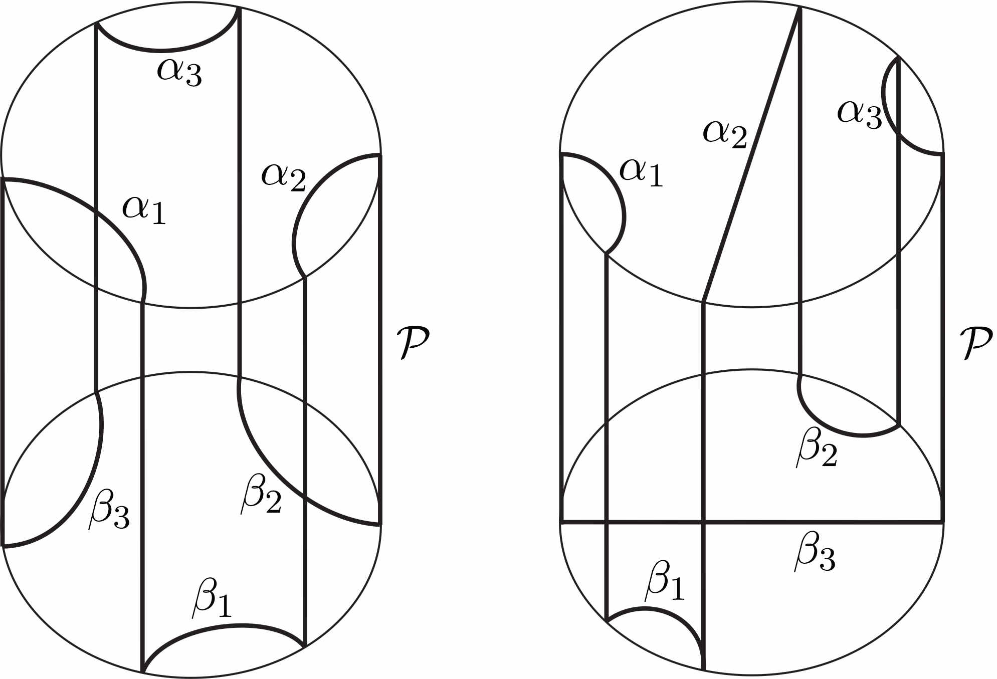
Figure 1: Examples of embedded admissible polygons at infinity.

Let us now describe the asymptotic behavior of finite total curvature minimal surfaces in $\operatorname{\mathbb{H}^{2}\times\mathbb{R}}$. A finite total curvature minimal surface ${\cal M}$ has finite topology, hence its ends are annular. Let $\Sigma$ be an annulus with the topology of $\operatorname{\mathbb{S}}^{1}\times(0,+\infty)$ and $X:\Sigma\rightarrow\operatorname{\mathbb{H}^{2}\times\mathbb{R}}$ be a proper minimal immersion. We call $M=X(\Sigma)$. It is proved in [12, Lemma 2.3] that, for $t_{0}>0$ large enough, $M\cap\{t>t_{0}\})$ (resp. $M\cap\{t<-t_{0}\})$) corresponds to a finite number of connected components $U_{1},...,U_{k}$ (resp. $V_{1},...,V_{k}$) in $\Sigma$. Finite total curvature implies that the curvature is uniformly bounded, converges uniformly to $0$ at infinity and the tangent planes become vertical. For each $U_{i}$, there exists a geodesic $\alpha_{i}\subset\operatorname{\mathbb{H}^{2}}$ such that $X(U_{i})$ is a horizontal Killing graph (see Definition 7 below) over $\alpha_{i}\times\mathbb{R}$ and $\partial_{\infty}X(U_{i})\subset\partial_{\infty}(\alpha_{i}\times\mathbb{R})$ (similarly for $X(V_{i})$, for some geodesic $\beta_{i}\subset\operatorname{\mathbb{H}^{2}}$). Moreover, for any vertical line $\{a\}\times[-1,1]\subset{\cal P}$, there exists a horodisk ${\mathcal{H}}$ with $\partial_{\infty}{\mathcal{H}}=\{a\}$ such that $M\cap({\mathcal{H}}\times\mathbb{R})$ corresponds to a finite number of connected components $W_{1},...,W_{k}$ in $\Sigma$. Each $X(W_{i})$ is a horizontal Killing graph over $\alpha\times\mathbb{R}$, where $\alpha\subset\operatorname{\mathbb{H}^{2}}$ is a geodesic having $a$ as an endpoint. Therefore, this proves that there exists an admissible polygon at infinity containing $\partial_{\infty}M$.

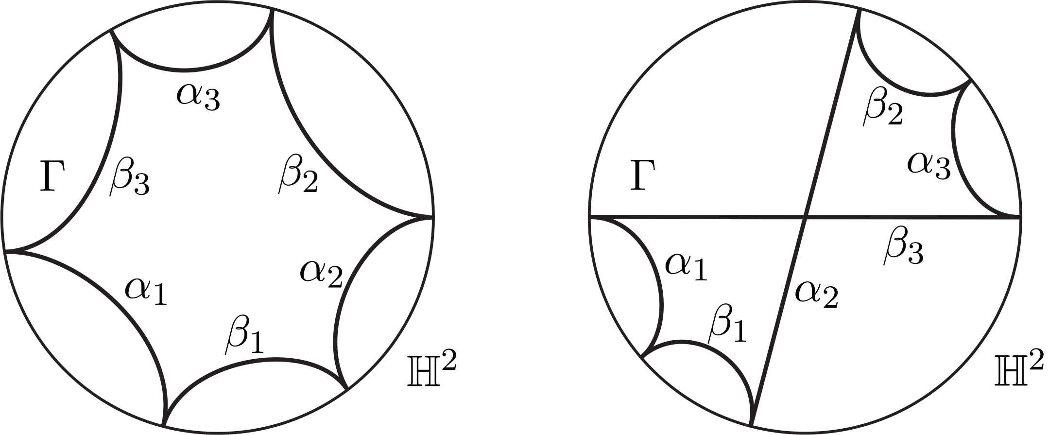
Figure 2: Projection over $\operatorname{\mathbb{H}^{2}}$ of the embedded admissible polygons at infinity in Figure 1.

The consequence of this behavior implies some classification theorems. If the projection of ${\cal P}$ is embedded and the surface ${\cal M}$ is embedded and has finite total curvature, we can begin the Alexandrov method of moving planes using horizontal slices coming from above, and we obtain that the only one-end complete embedded minimal surface ${\cal M}$ of finite total curvature with $\partial_{\infty}{\cal M}={\cal P}$ is a Jenkins-Serrin’s type graph over the ideal domain bounded by the projection of ${\cal P}$ (see Theorem 7). Another application is a Schoen’s type theorem for minimal annuli. Pyo [21] and Morabito-Rodríguez [18] have constructed minimal annuli with total curvature $4\pi$. The ends are asymptotic to two vertical geodesic planes $\alpha_{1}\times\operatorname{\mathbb{R}}$ and $\alpha_{2}\times\operatorname{\mathbb{R}}$. These annuli are called horizontal catenoids.

Theorem 1.

[12] A complete and connected minimal surface immersed in $\operatorname{\mathbb{H}^{2}\times\mathbb{R}}$ with nonzero finite total curvature and two ends, each one asymptotic to a vertical geodesic plane, is a horizontal catenoid.

The subtle thing is to define correctly the notion of asymptotic behavior at infinity of each end which permits to begin the Alexandrov method of moving planes. This will imply that the annulus has three geodesic planes of symmetry and is a geodesic bigraph (see Definition 8 below) on each of them. This will be enough to next conclude that the annulus is exactly a horizontal catenoid. The asymptotic hypothesis and finite total curvature assumed by the authors in Theorem 1 can be rewritten in a strong geometric hypothesis: Each end $M_{i}$ is assumed to be embedded and additionally a horizontal Killing graph outside a compact set on some vertical geodesic plane which converges uniformly to zero at infinity. These hypotheses are similar to the one used in the original work of R. Schoen for minimal surfaces in $\operatorname{\mathbb{R}}^{3}$ with two ends which are graphs over non compact domains of some planes. Alexandrov moving planes technique can be initiate at infinity with this behavior of $M_{i}$ (see [12]). We remark that R. Sa Earp and E. Toubiana obtains characterization of finite total curvature assuming stability, hence bounded uniform curvature at infinity.

Let us now introduce some definitions that we use to define a weaker notion of asymptoticity to an admissible polygon at infinity. We will define this asymptoticity in a topological meaning rather than a geometric one. For that, we fix an admissible polygon at infinity $\mathcal{P}$. Given a point $a$ at infinity of $\operatorname{\mathbb{H}^{2}}$, we consider a foliation given by a monotone family of horocylinders $\{{\mathcal{H}}(c)\}_{c\in\operatorname{\mathbb{R}}}$ with boundary $\{a\}\times[-1,1]$ at infinity.

Definition 3.

We say that $E$ is a horizontal sheet of $M\cap\bigcup_{c\geq c_{0}}{\mathcal{H}}(c)$, for some $c_{0}\in\operatorname{\mathbb{R}}$, if there exists a connected component $U$ of $X^{-1}(M\cap\{{{\mathcal{H}}(c)};c\geq c_{0}\})$ such that $E=X(U)$.

Definition 4.

We say that $E$ is a vertical sheet of $M\cap\{t>t_{0}\}$ (resp. $M\cap\{t<-t_{0}\}$), for some $t_{0}\in\operatorname{\mathbb{R}}$, if there exists a connected component $U$ of $X^{-1}(M\cap\{t>t_{0}\})$ (resp. $X^{-1}(M\cap\{t<-t_{0}\})$) such that $E=X(U)$.

We observe that a horizontal (resp. vertical) sheet $E$ is not necessarily a connected component of $M\cap\{{{\mathcal{H}}(c)};c\geq c_{0}\}$ (resp. $M\cap\{t>t_{0}\}$), since we do not assume $M$ necessarily embedded.

Definition 5.

We say that $M$ is asymptotic to an embedded admissible polygon at infinity ${\cal P}$ if $\partial_{\infty}M\subset{\cal P}$.

If ${\cal P}$ is not embedded, we say that $M$ is asymptotic to the admissible polygon at infinity ${\cal P}$ if $\partial_{\infty}M\subset{\cal P}$ and there exists $t_{0}>0$ such that the following assertions hold:

• For any vertical sheet $E$ of $M\cap\{t>t_{0}\}$, there exists some $i=1,...,k$ such that $\partial_{\infty}E\subset\partial_{\infty}(\alpha_{i}\times\operatorname{\mathbb{R}})$.

• For any vertical sheet $E$ of $M\cap\{t<-t_{0}\}$, there exists some $i=1,...,k$ such that $\partial_{\infty}E\subset\partial_{\infty}(\beta_{i}\times\operatorname{\mathbb{R}})$.

Remark 1.

There is no assumption on horizontal sheets in the last definition.

This notion of asymptoticity is topological. Next we define a stronger definition of asymptoticity which shares more geometric hypothesis.

Definition 6.

We say that ${M}$ is an asymptotic multigraph at infinity to ${\mathcal{P}}$ if $M$ is asymptotic to ${\mathcal{P}}$ and any vertical and horizontal sheet $E$ can be written outside a compact set as a horizontal graph over a domain of $\alpha\times\operatorname{\mathbb{R}}$, for some well chosen geodesic $\alpha$. The asymptotic multigraph is Killing (see definition 7) if $E$ is a graph along horocycles orthogonal to $\alpha\times\operatorname{\mathbb{R}}$ while the asymptotic multigraph is geodesic (see definition 8) if $E$ is a graph along geodesic orthogonal to $\alpha\times\operatorname{\mathbb{R}}$.

R. Sa Earp and E. Toubiana in [7, 8] has studied characterization of finite total curvature assuming stability. Stability say that the curvature on ends is bounded and using appropriate barriers, they can consider surfaces asymptotically multigraph at infinity as in the previous definition or graph on some slice $\operatorname{\mathbb{H}^{2}}\times\{0\}$.

In the following theorem we prove that the weak condition of asymptoticity is sufficient to prove finite total curvature. We provide uniform bound of the curvature by proving that properly immersed surfaces are asymptotically multigraph at infinity converging uniformly to zero.

Theorem 2.

Let ${\cal M}\subset\operatorname{\mathbb{H}^{2}\times\mathbb{R}}$ be a properly immersed minimal surface with finite topology and possibly compact boundary. Suppose that each end $M$ of ${\cal M}$ is asymptotic to an admissible polygon at infinity. Then $M$ is both a geodesic and Killing asymptotic multigraph at infinity and ${\cal M}$ has finite total curvature.

Theorem 2 is an immediate consequence of the next theorem using the fact that finite topology implies that each end $M$ is annular.

Theorem 3.

Let $M\subset\operatorname{\mathbb{H}^{2}\times\mathbb{R}}$ be a properly immersed minimal annulus with one compact boundary component $\partial M$ and asymptotic to an admissible polygon ${\cal P}$ at infinity. Then $M$ is an asymptotic geodesic and Killing multigraph at infinity and has finite total curvature.

As a consequence we have a characterization for finite total curvature minimal surfaces:

Theorem 4.

A complete minimal surface of $\operatorname{\mathbb{H}^{2}\times\mathbb{R}}$ has finite total curvature if and only if it is proper, has finite topology and each one of its ends is asymptotic to an admissible polygon at infinity.

We also obtain the following uniqueness result derived from Theorems 1 and 3:

Theorem 5.

A complete (and connected) minimal surface properly immersed in $\operatorname{\mathbb{H}^{2}\times\mathbb{R}}$ with two embedded ends $E_{1}$ and $E_{2}$ satisfying $\partial_{\infty}E_{1}\subset\partial_{\infty}(\alpha_{1}\times\operatorname{\mathbb{R}})$ and $\partial_{\infty}E_{2}\subset\partial_{\infty}(\alpha_{2}\times\operatorname{\mathbb{R}}),$ for some geodesics $\alpha_{1}$ and $\alpha_{2}$ in $\operatorname{\mathbb{H}^{2}}$, must be a horizontal catenoid.

We can also prove using Theorem 3 and Alexandrov’s moving planes method the following results:

Theorem 6.

Let $M$ be a (connected) properly immersed minimal surface in $\operatorname{\mathbb{H}^{2}\times\mathbb{R}}$ with a finite number of embedded ends $E_{1},\dots,E_{k}$ satisfying $\partial_{\infty}E_{i}\subset\partial_{\infty}(\alpha_{i}\times\operatorname{\mathbb{R}})$ for any $i=1,\dots,k$, where $\alpha_{1},\dots,\alpha_{k}$ denote complete geodesics in $\operatorname{\mathbb{H}^{2}}$ cyclically ordered. Then $M$ is a vertical bigraph symmetric with respect to a horizontal slice.

Theorem 7.

Let $M$ be a properly embedded minimal surface in $\operatorname{\mathbb{H}^{2}\times\mathbb{R}}$ with finite topology and one end asymptotic to an admissible polygon at infinity ${\cal P}$. Suppose that the vertical projection of ${\cal P}$ in $\operatorname{\mathbb{H}^{2}}$ is the boundary of a convex domain $\Omega$. Then $M$ is a vertical graph.

In particular, if $\alpha_{i}\times\{1\}$ and $\beta_{i}\times\{-1\}$, with $i=1,\dots,k$, are the edges of ${\cal P}$ then:

1. $\sum_{i=1}^{k}|\alpha_{i}|=\sum_{i=1}^{k}|\beta_{i}|$; and

2. for any inscribed polygonal domain $D$ in $\Omega$, $\sum_{i=1}^{k}|\alpha_{i}\cap\partial D|=\sum_{i=1}^{k}|\beta_{i}\cap\partial D|$,

where $|\bullet|$ denotes the hyperbolic length of the curve $\bullet$.

Open problems. Does it exist a one-end torus of finite total curvature? Does it exist one whose associated polygon at infinity ${\cal P}$ does not project on some embedded ideal polygonal (see Figure 1, right)? What about higher genus? More generally, can we study the moduli space of finite total curvature minimal surfaces in function of the space of admissible polygons at infinity?

Theorem 2 has a natural extension to $\operatorname{\widetilde{\rm PSL}_{2}(\operatorname{\mathbb{R}},\tau)}$. These simply-connected homogeneous manifolds can be viewed as $\operatorname{\mathbb{D}}\left(\sqrt{\frac{-4}{\kappa}}\right)\times\operatorname{\mathbb{R}}$, where $\operatorname{\mathbb{D}}\left(\sqrt{\frac{-4}{\kappa}}\right)=\{x^{2}+y^{2}\leq-4/\kappa\}$, endowed with the following metric:

$$g=\lambda^{2}(dx^{2}+dy^{2})+(\tau\lambda(ydx-xdy)+dz)^{2},$$

where $\lambda=\frac{1}{1+\frac{\kappa}{4}(x^{2}+y^{2})}$. R. Younes [27] first studied the Jenkins-Serrin problem on compact domains of the basis and S. Melo [17] proved the existence of complete minimal graphs on ideal domains.

The curvature of a minimal surface in $\operatorname{\widetilde{\rm PSL}_{2}(\operatorname{\mathbb{R}},\tau)}$ satisfies $K\leq\tau$ and does not have necessarily a negative sign. Hence it seems more difficult to prove theorems involving the Gaussian curvature. However in [20] Minh Nguyen proves that minimal surfaces with uniform bounded curvature which are geodesic asymptotic multigraphs have finite total curvature

$$\int_{\Sigma}|K|dA\leq C.$$

Using this property we can prove Theorem 3 in $\operatorname{\widetilde{\rm PSL}_{2}(\operatorname{\mathbb{R}},\tau)}$:

Theorem 8.

Let $M\subset\operatorname{\widetilde{\rm PSL}_{2}(\operatorname{\mathbb{R}},\tau)}$ be a properly immersed minimal annulus with one compact boundary component $\partial M$ and asymptotic to an admissible polygon ${\cal P}$ at infinity. Then $M$ is an asymptotic Killing and geodesic multigraph and has finite total curvature.

This theorem implies that the complete graphs defined over ideal polygonal domains of $\{z=0\}$ constructed by Melo [17] have finite total curvature. Collin, Nguyen and the first author have constructed in [1], via variational methods, a horizontal catenoid in $\operatorname{\widetilde{\rm PSL}_{2}(\operatorname{\mathbb{R}},\tau)}$ asymptotic to two vertical geodesic planes. As a consequence of Theorem 8, this annulus has finite total curvature.

Remark 2.

It is not known if a complete finite total curvature annular end in $\operatorname{\widetilde{\rm PSL}_{2}(\operatorname{\mathbb{R}},\tau)}$ must be asymptotic to an admissible polygon at infinity.

2 Preliminaries

There are several models for the 2-dimensional hyperbolic space $\operatorname{\mathbb{H}^{2}}$. If we use the Poincaré disk model for the 2-dimensional hyperbolic space, then the space $\operatorname{\mathbb{H}^{2}}$ is given by

$$\mathbb{H}^{2}=\{(x,y)\in\operatorname{\mathbb{R}}^{2};\ x^{2}+y^{2}<1\}$$

with the hyperbolic metric $g_{-1}=\frac{4}{(1-x^{2}-y^{2})^{2}}g_{0},$ where $g_{0}$ denotes the Euclidean metric in $\operatorname{\mathbb{R}}^{2}.$ In this model, the asymptotic boundary $\partial_{\infty}\mathbb{H}^{2}$ of $\mathbb{H}^{2}$ can be identified with the unit circle. There are different models to describe the asymptotic boundary of $\operatorname{\mathbb{H}^{2}\times\mathbb{R}}$. In this paper we consider the product compactification obtained as the product of the compactifications of each of the factors.

If we consider the half-plane model for $\operatorname{\mathbb{H}^{2}}$, then the space $\operatorname{\mathbb{H}^{2}}$ is given by

$$\operatorname{\mathbb{H}^{2}}=\{(x,y)\in\operatorname{\mathbb{R}}^{2};y>0\},$$

endowed with the metric $g_{-1}=\frac{1}{y^{2}}g_{0}$

To describe the homogeneous $3$-manifold $\operatorname{\widetilde{\rm PSL}_{2}(\operatorname{\mathbb{R}},\tau)}$ we use the half-plane model for $\operatorname{\mathbb{H}^{2}},$ since we are interested in horizontal graphs. Hence, in Euclidean coordinates, we have

$$\operatorname{\widetilde{\rm PSL}_{2}(\operatorname{\mathbb{R}},\tau)}=\operatorname{\mathbb{R}}^{2}_{+}\times\operatorname{\mathbb{R}}=\{(x,y,t)\in\operatorname{\mathbb{R}}^{3};y>0\},$$

endowed with the Riemannian metric

$$ds^{2}=\frac{1}{y^{2}}g_{0}+\left(dt-\frac{2\tau}{y}dx\right)^{2}.$$

The orthonormal frame $B=\{E_{1},E_{2},E_{3}\}$ in $\operatorname{\widetilde{\rm PSL}_{2}(\operatorname{\mathbb{R}},\tau)}$ is given by

$$E_{1} =y\partial_{x}+2\tau\partial_{t}, E_{2} =y\partial_{y} E_{3} =\partial_{t}$$

and satisfies $[E_{1},E_{3}]=[E_{2},E_{3}]=0$, $[E_{1},E_{2}]=-E_{1}+2\tau E_{3}$, so the Levi-Civita connection is given by

$$\begin{array}[]{lll}\overline{\nabla}_{E_{1}}E_{1}=E_{2},&\overline{\nabla}_{E_{1}}E_{2}=-E_{1}+\tau E_{3},&\overline{\nabla}_{E_{1}}E_{3}=-\tau E_{2},\\ \overline{\nabla}_{E_{2}}E_{1}=-\tau E_{3},&\overline{\nabla}_{E_{2}}E_{2}=0&\overline{\nabla}_{E_{2}}E_{3}=\tau E_{1},\\ \overline{\nabla}_{E_{3}}E_{1}=-\tau E_{2},&\overline{\nabla}_{E_{3}}E_{2}=\tau E_{1},&\overline{\nabla}_{E_{3}}E_{3}=0.\end{array}$$ (2.1)

From now on, $N^{3}$ will denote $\operatorname{\mathbb{H}^{2}\times\mathbb{R}}$ or $\operatorname{\widetilde{\rm PSL}_{2}(\operatorname{\mathbb{R}},\tau)}$.

We consider a vertical geodesic plane $\alpha\times\operatorname{\mathbb{R}}=\{(x,y,t)\in\operatorname{\mathbb{R}}^{2}_{+}\times\operatorname{\mathbb{R}};x=0\}$ and we define different notions of horizontal graphs over $\alpha\times\operatorname{\mathbb{R}}$:

Definition 7.

A surface ${\cal M}\subset N^{3}$ is said to be a horizontal Killing graph over $\alpha\times\operatorname{\mathbb{R}}$, if ${\cal M}$ is the graph of a function $f:\Omega\subset\alpha\times\operatorname{\mathbb{R}}\to\operatorname{\mathbb{R}}$ along horizontal horocycles, that is, ${\cal M}=X(\Omega),$ where

$$X(y,t)=(f(y,t),y,t).$$

The parabolic isometry preserving the point at infinity $(0,0,0)$ induces a Killing field into the ambient space and a positive Jacobi field on the graph ${\cal M}$. A well known result by Fischer-Colbrie and Schoen [9] assures that the existence of a positive Killing field on the surface ${\cal M}$ gives that ${\cal M}$ is stable, hence has bounded curvature away from its boundary by an uniform estimate (R. Schoen [26]).

Definition 8.

A surface ${\cal M}\subset N^{3}$ is a horizontal geodesic graph over $\alpha\times\operatorname{\mathbb{R}}$, if ${\cal M}$ is the graph of a function $f:\Omega\subset\alpha\times\operatorname{\mathbb{R}}\to\operatorname{\mathbb{R}}$ along horizontal geodesics orthogonal to $\alpha\times\operatorname{\mathbb{R}},$ that is, ${\cal M}=X(\Omega),$ where

$$X(y,t)=(e^{y}\tanh(f),e^{y}\operatorname{sech}(f),t+2\tau\arcsin(\tanh(f))).$$

The mean curvature operator associated to this notion of graphs has been studied in [20]. In this case, we cannot use stability to assure that a geodesic graph has bounded curvature away from its boundary but we can apply a blow up argument inspired by Rosenberg, Souam and Toubiana [24]:

Lemma 1.

A horizontal geodesic graph ${\cal M}$ over $\alpha\times\operatorname{\mathbb{R}}$ has uniform bounded curvature.

Proof.

This blow up argument is standard. Suppose ${\cal M}$ does not have bounded curvature. Then there exists a divergent sequence $\{p_{n}\}$ in ${\cal M}$ such that $|A(p_{n})|\geq n,$ where $A$ denotes the second fundamental form of ${\cal M}$. Denote by $C_{n}$ the connected component of $p_{n}$ in an extrinsec ball $\bar{B}(p_{n},\delta)\cap{\cal M}$, for some $\delta>0$. Consider the function $f_{n}:C_{n}\rightarrow\operatorname{\mathbb{R}}$ given by

$$f_{n}(q)=d(q,\partial C_{n})|A(q)|,$$

where $d$ is the extrinsic distance. The function $f_{n}$ restricted to the boundary of $C_{n}$ is identically zero and $f_{n}(p_{n})=\delta|A(p_{n})|>0.$ Then $f_{n}$ attains a maximum in a point $q_{n}$ of the interior. Hence $\delta|A(q_{n})|\geq d(q_{n},\partial C_{n})|A(q_{n})|=f_{n}(q_{n})\geq f_{n}(p_{n})=\delta|A(p_{n})|\geq\delta n,$ what yields $|A(q_{n})|\geq n.$

Now consider $r_{n}=\frac{d(q_{n},\partial C_{n})}{2}$ and denote by $B_{n}$ the connected component of $q_{n}$ in $\bar{B}(q_{n},r_{n})\cap{\cal M}.$ We have $B_{n}\subset C_{n}.$ If $q\in B_{n},$ then $f_{n}(q)\leq f_{n}(q_{n})$ and

$$\begin{array}[]{rcl}d(q_{n},\partial C_{n})&\leq&d(q_{n},q)+d(q,\partial C_{n})\\ &&\\ &\leq&\frac{d(q_{n},\partial C_{n})}{2}+d(q,\partial C_{n})\\ &&\\ \Rightarrow d(q_{n},\partial C_{n})&\leq&2d(q,\partial C_{n}).\par\end{array}$$

Hence we conclude that $|A(q)|\leq 2|A(q_{n})|.$

Call $g$ the metric on $N^{3}$ in the half space model. The graph ${\cal M}$ is transverse to a foliation of horocylinders (vertical planes in the euclidean model). Consider ${\cal M}_{n}$ the homothety of $B_{n}$ by $\lambda_{n}=|A(q_{n})|$. We obtain at the limit a complete minimal surface $\widetilde{\cal M}$ in $\operatorname{\mathbb{R}}^{3}$ which is transversal to the limit of the foliation of circle dilated by the homothety. This foliation is converging to parallel line in $\operatorname{\mathbb{R}}^{3}$, hence $\widetilde{\cal M}$ is a complete graph of $\operatorname{\mathbb{R}}^{3}$, which is flat by Bernstein theorem, a contradiction.

∎

We now introduce some techniques we will use in this paper. Roughly speaking we will use the hypothesis on the asymptotic boundary of the ends to construct barriers which will constrain the geometry of the ends locally in some union of vertical slabs (i.e. the region bounded by the equidistant planes at a fixed distance from a vertical geodesic plane). After that we will study the geometry of subdomains of ends which are contained in some vertical slab with small width. We will use what we call Dragging Lemma, a technique developped by Collin, Hauswirth and Rosenberg in [3, 4], to prove that the end is a horizontal multigraph, hence has uniform bounded curvature at infinity using stability or Lemma 1. Then we will prove that the property on the boundary at infinity implies that the ends have finite total curvature.

2.1 Family of barriers: ${\cal C}(h)$ and $S_{h}$

Given $h\in(0,\pi)$, there is a one parameter family of rotationally invariant surfaces ${\mathcal{C}}(h)$ called vertical catenoids in $\operatorname{\mathbb{H}^{2}}Ê\times\operatorname{\mathbb{R}}$, where $h$ is the total height of the examples. The boundary of ${\mathcal{C}}(h)$ at infinity consists of two horizontal circles at height $t=h/2$ and at $t=-h/2$. We denote by $r_{h}$ the size of the neck (the length of the curve ${\cal C}(h)\cap\{t=0\}$) of these examples. When $h\to\pi$, then $r_{h}\to\infty$ and the surface disappears at infinity. When $h\to 0$, $r_{h}\to 0$ and the catenoids converge to the horizontal section $\operatorname{\mathbb{H}^{2}}\times\{0\}$ with degree two.

In $\operatorname{\widetilde{\rm PSL}_{2}(\operatorname{\mathbb{R}},\tau)}$, Peñafiel [19] has studied rotationally invariant families of minimal surfaces. There are vertical catenoids whose boundary at infinity consists of two horizontal circles at heights $\pm h$, for any $h\in(0,\pi\sqrt{1+4\tau^{2}})$, with $r_{h}\to\infty$ as $h\to\pi\sqrt{1+4\tau^{2}}$.

Applying a maximum principle with these families of rotationally invariant surfaces we have the following non existence property:

Lemma 2.

There is no minimal surface ${\cal M}$ in $N^{3}$ with compact instersection with

$$S=\{-\pi\sqrt{1+4\tau^{2}}/2\leq t\leq\pi\sqrt{1+4\tau^{2}}/2\}$$

and boundary $\partial{\cal M}\cap S=\emptyset$.

Given $h>\pi$ and a geodesic $\alpha\subset\operatorname{\mathbb{H}^{2}}$ with endpoints $a_{1},a_{2}\in\partial_{\infty}\operatorname{\mathbb{H}^{2}}$, we will consider the minimal surface $S_{h}\subset\operatorname{\mathbb{H}^{2}}\times(0,h)$, first introduced by Hauswirth [11] then by Sa Earp and Toubiana [25] and Daniel [6] (see also Mazet, Rodríguez and Rosenberg [15, 16]). This minimal surface is a vertical bigraph with respect to $\operatorname{\mathbb{H}^{2}}\times\{h/2\},$ is invariant by horizontal translations along $\alpha$ and its asymptotic boundary is $(\eta\times\{0,h\})\cup(\{a_{1},a_{2}\}\times[0,h])$, where $\eta$ is an arc in $\partial_{\infty}\operatorname{\mathbb{H}^{2}}$ with endpoints $a_{1},a_{2}$ (see Figure 3 (left)). We remark that for each $t\in(0,h)$, $S_{h}\cap(\operatorname{\mathbb{H}^{2}}\times\{t\})$ is an equidistant curve to $\alpha\times\{t\}$. Moreover, when $h$ goes to $+\infty$, the distance between $S_{h}\cap(\operatorname{\mathbb{H}^{2}}\times\{h/2\})$ and $\alpha\times\{h/2\}$ goes to zero; in fact, the graph $S_{h}\cap\{0<t<h/2\}$ converges to the minimal graph $S_{\infty}$ defined over the domain bounded by $\alpha\cup\eta$ with boundary values $+\infty$ over $\alpha$ and 0 over $\eta$ (see Figure 3 (right)).

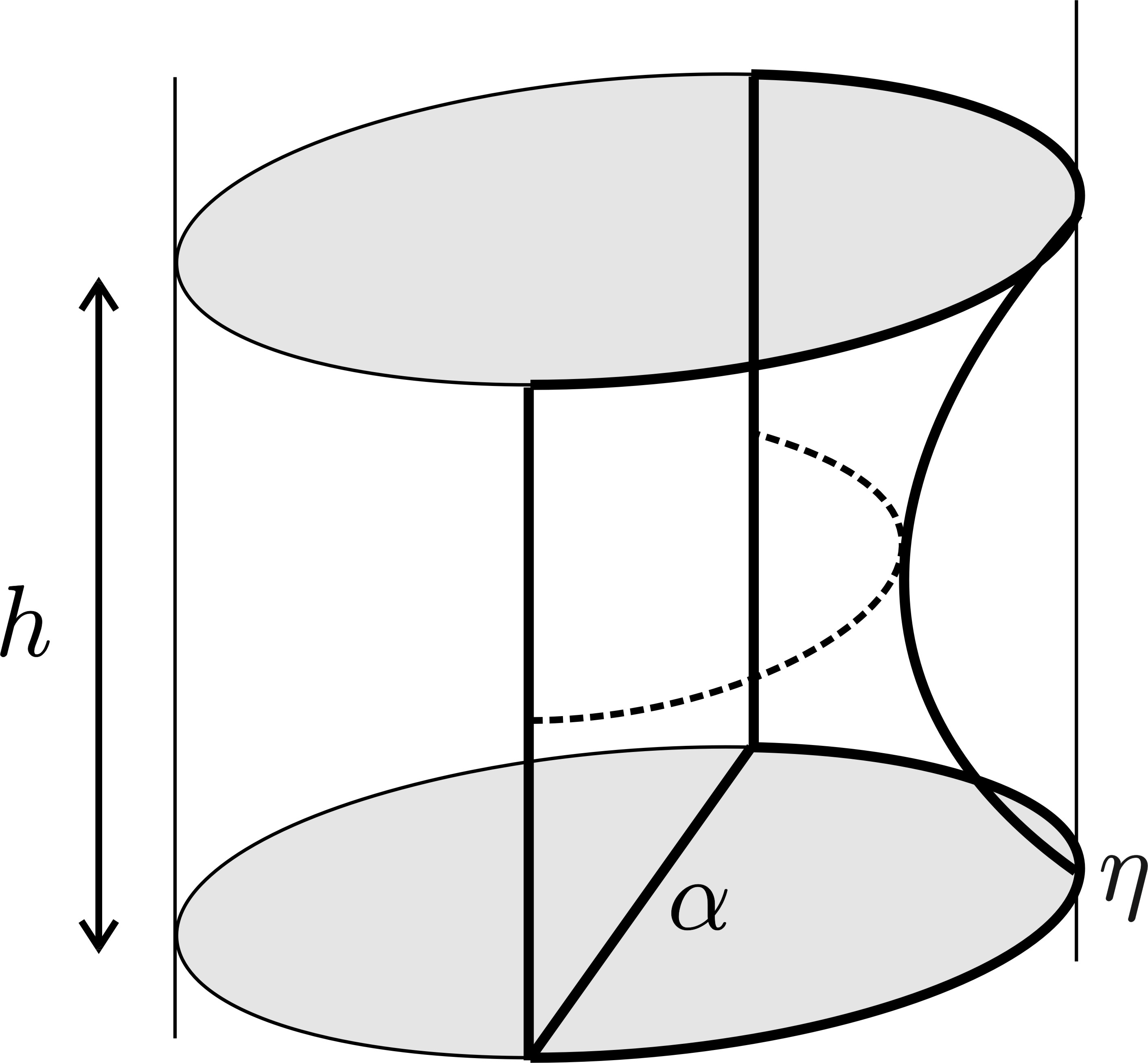
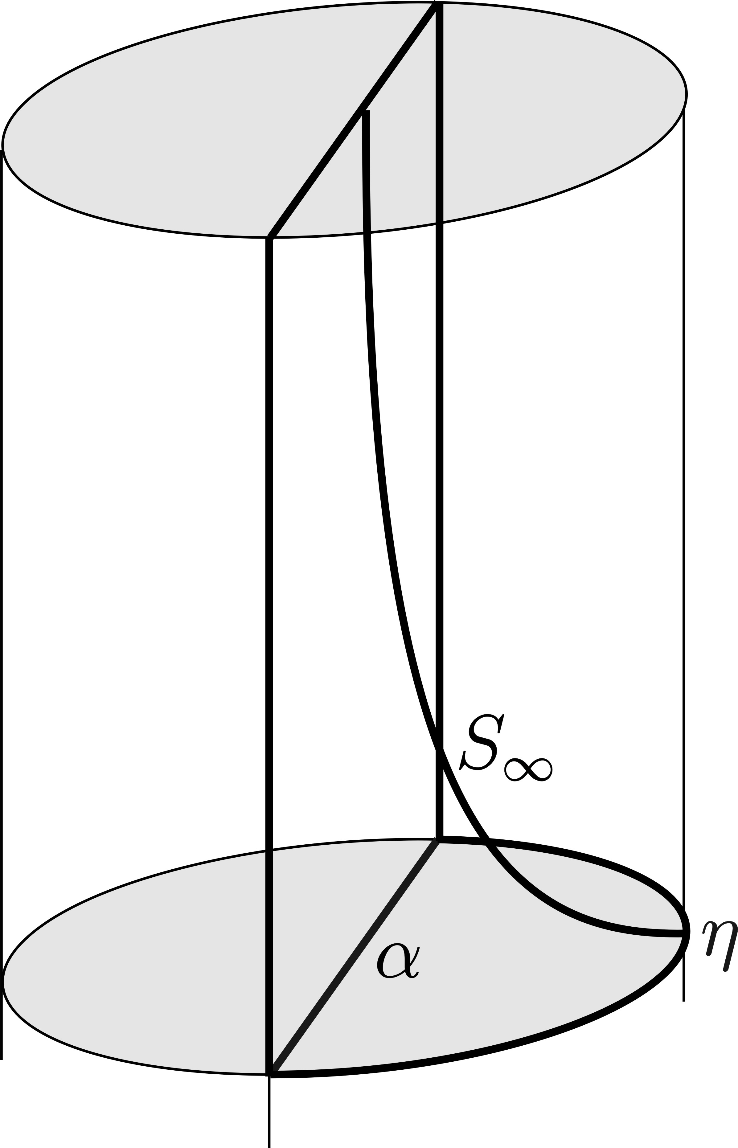
Figure 3: Left: Minimal surface $S_{h}$; Right: Minimal surface $S_{\infty}$

In $\operatorname{\widetilde{\rm PSL}_{2}(\operatorname{\mathbb{R}},\tau)}$, Folha and Peñafiel [10] have obtained similar minimal disks $S_{h}$, for any $h>\pi\sqrt{1+4\tau^{2}}$, and $S_{\infty}$.

2.2 The Dragging Lemma

This refer as a technique of topological continuation of an arc into a minimal surface immersed in an arbitrary three manifold $N^{3}$ (in our context, $N^{3}$ is $\operatorname{\mathbb{H}^{2}}\times\operatorname{\mathbb{R}}$ or $\operatorname{\widetilde{\rm PSL}_{2}(\operatorname{\mathbb{R}},\tau)}$). We deal with a geometrical situation where the immersed minimal surface ${\cal M}=X(\Sigma)$ is simply connected and is contained in a slab $S$ with small width. In this situation, we consider a compact annulus $A_{0}$ with boundary outside the slab, intersecting ${\cal M}$ in its interior with $A_{0}\cap\partial{\cal M}=\emptyset$. The two components of the boundary of $A_{0}$ are contained in different connected components of $N^{3}\setminus S$.

Now we move the annulus $A_{0}$ by using an ambient isometry and we consider $t\to A(t)$ the position of the translated annulus moved in a ${\mathcal{C}}^{1}$-way such that $A(t)\cap\partial{\cal M}=\emptyset$ and $\partial A(t)\cap{\cal M}=\emptyset$. The maximum principle says that $A(t)\cap{\cal M}$ cannot be empty, otherwise there would be a last point of contact between these two surfaces, a contradiction. Then if $p$ is a point in the intersection at $t=0$, we can construct a path $\alpha(t)$ with endpoint $p$ such that $\alpha(t)\in A(t)\cap{\cal M}$. This path can be continued while $A(t)$ does not meet the boundary of ${\cal M}$. This path can be constructed in a ${\mathcal{C}}^{1}$-way and monotonically. This is a consequence of the Dragging Lemma:

Lemma 3 (Dragging Lemma [3, 4]).

Let $g:\Sigma\to N^{3}$ be a properly immersed minimal surface in a complete $3$-manifold $N^{3}$. Let $A$ be a compact surface (perhaps with boundary) and $f:A\times[0,1]\to N^{3}$ be a ${\mathcal{C}}^{1}$-map such that $f(A\times\{t\})=A(t)$ is a minimal immersion for $0\leq t\leq 1$. If $\partial(A(t))\cap g(\Sigma)=\emptyset$ for $0\leq t\leq 1$ and $A(0)\cap g(\Sigma)\neq\emptyset$, then there is a ${\mathcal{C}}^{1}$ path $\alpha(t)$ in $\Sigma$ such that $(g\circ\alpha)(t)\in A(t)\cap g(\Sigma)$ for $0\leq t\leq 1$. Moreover, we can prescribe any initial value $(g\circ\alpha)(0)\in A(0)\cap g(\Sigma)$.

2.3 The minimal annulus $A_{0}$ and an application of the Dragging Lemma

We consider a slab $\mathcal{R}_{d}$ in $\operatorname{\mathbb{H}^{2}}\times\operatorname{\mathbb{R}}$ bounded by some equidistant planes $P^{d}$ and $P^{-d}$ to some vertical plane). We will study the geometry of subdomains of ends which are contained in some vertical slab with small width. We will use what we call Dragging Lemma, a technique developped by Collin, Hauswirth and Rosenberg in [3, 4], to prove that the end is a horizontal multigraph, hence has uniform bounded curvature at infinity using stability or Lemma 1. Then we will prove that the property on the boundary at infinity implies that the ends have finite total curvature.

Lemma 4.

Given $d>0$ small enough, there exists a compact stable minimal annulus $A_{0}$ in $\operatorname{\mathbb{H}^{2}}Ê\times\operatorname{\mathbb{R}}$ bounded by two large enough circles (in exponential coordinates) $\eta_{+}\subset P^{d}$ and $\eta_{-}\subset P^{-d}$. This annulus $A_{0}$ is symmetric with respect to the vertical geodesic plane $\alpha_{0}\times\operatorname{\mathbb{R}}$ and the unit normal vector to $A_{0}$ along the intersection curve $A_{0}\cap(\alpha_{0}\times\operatorname{\mathbb{R}})$, which is convex, takes all directions in the plane $\alpha_{0}\times\operatorname{\mathbb{R}}$.

Let us denote by $\xi$ the geodesic that joins the centers of $\eta_{+}$ and $\eta_{-},$ and by $q_{1}$ the point $\xi\cap(\alpha_{0}\times\operatorname{\mathbb{R}}).$ Assume the circles $\eta_{+}$ and $\eta_{-}$ are sufficiently close so that $\xi\cap A_{0}=\emptyset.$

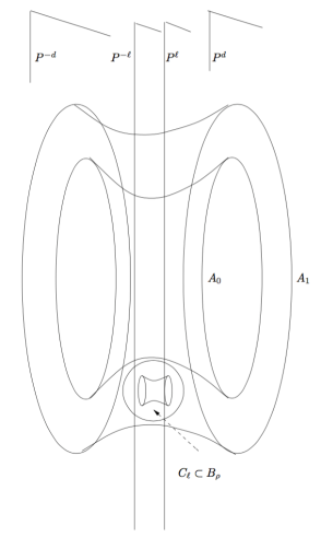
Figure 4: Annuli $A_{0}$ and $C_{\ell}$

By stability, there exist $\delta>0$ and a foliation of a (closed) neighborhood of $A_{0}$ in the slab $\mathcal{R}_{d}$ bounded by the vertical planes $P^{d}\cup P^{-d}$ given by compact annuli $A_{s}$, for $-\delta\leq s\leq\delta$, each $A_{s}$ with boundary $\eta_{s}\cup\eta_{-s}$, where $\eta_{s}$ and $\eta_{-s}$ are equidistant curves at distance $s$ from $\eta_{+}$ and $\eta_{-},$ respectively. $A_{0}$ separates the slab $\mathcal{R}_{d}$ in two connected components, one interior compact region $A_{0}^{-}$ and the other one $A_{0}^{+},$ the outside region of $\mathcal{R}_{d}\setminus A_{0}$ which is non compact. Let us assume that $A_{s}\subset A_{0}^{+}$ if $s>0$. Let us write

$${\rm Tub}^{+}(A_{0})=\cup_{s\in[0,\delta]}A_{s}\quad\mbox{and}\quad{\rm Tub}^{-}(A_{0})=\cup_{s\in[-\delta,0]}A_{s}.$$

There exists a small constant $\rho>0$ such that, for any point $q\in A_{\delta/2}\cap(\alpha_{0}\times\operatorname{\mathbb{R}})$ (resp. $A_{-\delta/2}\cap(\alpha_{0}\times\operatorname{\mathbb{R}})$), the geodesic open ball $B_{\rho}(q)$ centered at $q$ with radius $\rho$ is contained in Tub${}^{+}(A_{0})$ (resp. Tub${}^{-}(A_{0})$) and any such $B_{\rho}(q)$ contains a small compact minimal annulus $C_{\ell}$ bounded by two circles (in exponential coordinates) contained in $B_{\rho}(q)\cap(P^{\ell}\times\operatorname{\mathbb{R}})$ and $B_{\rho}(q)\cap(P^{-\ell}\times\operatorname{\mathbb{R}})$, for some small $\ell>0$ (see Figure 4). We further can take $\rho>0$ satisfying:

1. $3\rho<\mbox{dist}(A_{0},\xi),$

2. $B_{2\rho}(q_{1})\cap\mbox{Tub}^{-}(A_{0})=\emptyset,$ where $q_{1}=\xi\cap(\alpha_{0}\times\operatorname{\mathbb{R}})$.

Lemma 5.

If there is a compact minimal surface ${\cal M}\subset\mathcal{R}_{\ell}\cap A_{0}^{+}$ with $\partial{\cal M}\subset A_{0}$, then ${\cal M}$ is actually a subdomain of $A_{0}$.

Proof.

Let $K$ be the compact set containing $A_{0}$ and bounded by horizontal and vertical planes. The surface ${\cal M}$ cannot have points outside $K$ without having an interior point of contact with a horizontal slice or a vertical geodesic plane, contradicting the maximum principle. Moreover, ${\cal M}$ cannot be entirely contained in ${\rm Tub}^{+}(A_{0})$, otherwise there would be a last leaf of the foliation having a last point of contact, a contradiction again with the maximum principle.

However, it still remains some room between the last annulus of the foliation $A_{s}$ and $\partial K$. But we can find a catenoid $C_{\ell}$ which intersects ${\cal M}$ without intersecting the boundary by choosing correctly the point $q$ on the waist circle of $A_{\delta/2}$ and we could use the Dragging Lemma to find points of ${\cal M}$ outside $K$ by moving $C_{\ell}$ into $A_{\delta/2}^{+}$. This proves that ${\cal M}$ has to be contained in $A_{0}$. ∎

In the half-space model of $\operatorname{\mathbb{H}^{2}}$ with orthonormal basis $(e_{1},e_{2})$ and the geodesic $\alpha_{0}$ represented by the half-line $\{x=0\}$, the equidistant curves $\alpha_{-d}$ and $\alpha_{d}$ are half-lines making with $\{x=0\}$ angles $\pm\theta$, being $\sin\theta=\tanh d$. In this model, translations fixing the point at infinity $(0,0)$ correspond to homoteties and rotations centered at $(0,0)$. Any one of these translations corresponds to a horizontal isometry in $\operatorname{\mathbb{H}^{2}\times\mathbb{R}}$ that produces a Killing field $Y$ which is tangent to $A_{0}$ along the curve $A_{0}\cap(\alpha_{0}\times\operatorname{\mathbb{R}})$.

Given a point $p\in\mathcal{R}_{d}$ of a surface with an unit normal vector $N(p)$ orthogonal to $Y(p)$, there exists an isometry ${\cal I}$ such that ${\cal I}(A_{0})$ is an annulus passing through $p\in S$, with $N(p)$ as its unit normal vector. That isometry is nothing but a combination of horizontal and vertical translations keeping the boundary outside $\mathcal{R}_{d}$.

Concerning the same result in $\operatorname{\widetilde{\rm PSL}_{2}(\operatorname{\mathbb{R}},\tau)}$, we need the existence of a compact stable minimal annulus $A_{0}$ with boundary curves outside the vertical slab $\mathcal{R}_{d}$ bounded by $P^{-d}\cup P^{d}$ and the existence of a non nulhomotopic curve $\gamma$ in $A_{0}$ along where the Killing vector $Y$ is tangent to the annulus. Moreover we need to prove that $\gamma$ is at least at distance $2d$ from the boundary $\partial A_{0}$ in such a way that $\partial{\cal I}(A_{0})\cap(P^{-d}\cup P^{d})=\emptyset$, when ${\cal I}(A_{0})$ passes through an arbitrary point $p$ of $\mathcal{R}_{d}$.

Lemma 6.

Given $d>0$ small enough, there exists a compact stable minimal annulus $A_{0}$ in $\operatorname{\widetilde{\rm PSL}_{2}(\operatorname{\mathbb{R}},\tau)}$ bounded by two large enough circles (in exponential coordinates) $\eta_{+}\subset P^{d}$ and $\eta_{-}\subset P^{-d}$. This annulus $A_{0}$ has a non nul homotopic curve $\gamma$ where the vector field $Y$ is tangent to $A_{0}$. This curve $\gamma$ is at horizontal distance at least $2d$ from the boundary $\partial A_{0}$.

Proof.

We need to prove that, for $d>0$ small enough, there is a compact stable annulus which is almost symmetric in an Euclidean sense. In [1], the authors constructed a minimal annulus which is asymptotic to two vertical planes $\alpha_{\epsilon}\times\operatorname{\mathbb{R}}$ and $\alpha_{-\epsilon}\times\operatorname{\mathbb{R}}$ in $\operatorname{\widetilde{\rm PSL}_{2}(\operatorname{\mathbb{R}},\tau)}$. Let $2\epsilon$ be the distance between these asymptotic planes and let $\alpha_{0}\times\operatorname{\mathbb{R}}$ be the plane of Euclidean symmetry between the two planes. When $\epsilon\to 0$, the set of annuli are converging to the double covering of $\alpha_{0}\times\operatorname{\mathbb{R}}$, and the waist circle of these complete annuli is shrinking to a point. Since the curvature blows-up, we can use an Euclidean homothety to modify the model and see forming a convergent sequence of bounded curvature annuli which converge (see [1] for details) to a catenoid. Since during the process, the plane $\alpha_{0}\times\operatorname{\mathbb{R}}$ is transverse to the annuli, the limit is a horizontal catenoid with horizontal flux. Hence for $\epsilon$ small enough the complete annulus has almost a plane of symmetry in the Euclidean model. We can consider a compact stable subdomain of this example to insure that the boundary is at non zero distance from the curve $\gamma$. ∎

2.4 Conformal minimal immersion and finite total curvature.

In this section we summarize some of the results proved in [13, 12]. Let ${\cal M}$ be a complete Riemann surface and $X=(F,h):{\Sigma}\to\operatorname{\mathbb{H}^{2}\times\mathbb{R}}$ be a conformal minimal immersion with ${\cal M}=X(\Sigma)$. We take a local conformal coordinate $z$ on $\Sigma$. The Hopf differential associated to the harmonic map $F:\Sigma\to\operatorname{\mathbb{H}^{2}}$ is a quadratic holomorphic differential globally defined on $\Sigma$ and can be written as $Q=\phi(z)dz^{2}$. The real harmonic function $h:\Sigma\to\operatorname{\mathbb{R}}$ can be recovered as $h=2{\rm Re}\int-2i\sqrt{\phi}\,dz$.

If ${\cal M}$ has finite total curvature, then the immersion is proper and by Huber’s Theorem, any end $M$ of the surface ${\cal M}$ can be conformally parameterized by ${\cal U}=\{z\in\operatorname{\mathbb{C}}\ ;\ |z|\geq R\}$, for some $R>1$ with $X({\cal U})=M$. The Hopf differential $Q$ extends meromorphically to the puncture $z=\infty$ and we can write $\sqrt{\phi(z)}=\sum_{k\geq 1}a_{k}\,z^{-k}+P(z)$, where $a_{k}\in\operatorname{\mathbb{C}}$ for any $k\geq 1$ and $P$ is a polynomial of degree $m\geq 0$. We say that the end $M$ has degree $m$.

The fact that $\phi$ extends meromorphically at the puncture implies that the surface is transverse to any horizontal plane $\{h(z)=\pm t\}$, for $t\geq t_{0}>0$ large enough and ${\cal U}\cap X^{-1}(\{t=t_{0}\})$ has a finite number of connected components. The image by $X$ of each one of these components is the boundary of a vertical sheet $E$ contained in $X({\cal U})$.

For any conformal immersion, there is a function $\omega:\Sigma\to\operatorname{\mathbb{R}}$ such that the third coordinate of the unit normal vector is given by

$$n_{3}=\tanh\omega.$$

This function corresponds to a Jacobi field on ${\cal M}$, hence $\omega$ satisfies the differential elliptic equation

$$\Delta_{0}\omega-2|\phi|\sinh(2\omega)=0,$$

where $\Delta_{0}$ denotes the Laplacian in the Euclidean metric $|dz|^{2}$. The conformal metric induced by the immersion is given by

$$ds^{2}=4\cosh^{2}\omega|\phi||dz|^{2}.$$

Lemma 7.

[13, 12] If $\phi$ is without zeroes on ${\cal U}$, the function $\omega$ satisfies the uniform decay estimate

$$|\omega(p)|Ê\leq Ce^{{\rm dist}(p,\partial{\cal U})},$$

where ${\rm dist}(p,\partial{\cal U})$ is the distance with the flat metric $|dw|^{2}=|\phi(z)||dz|^{2}$.

A finite total curvature end satisfies the hypothesis of this lemma. If we reparametrize a vertical sheet $E$ of $X({\cal U})$ by its third coordinate factor we obtain a conformal parameter $w=u+it$ with $\phi(w)=\frac{1}{4}(dw)^{2}$. In this parametrization the level set $\Gamma_{h}=E\cap\{t=t_{1}\}$ is a curve parametrized by $u\to F(u,t_{1})$ with geodesic curvature in $\operatorname{\mathbb{H}^{2}}$ given by (see [11]):

$$k_{g}=\frac{-\partial_{u}\omega}{\cosh\omega}\hbox{ and }|\partial_{u}F(u,t_{1})|_{\operatorname{\mathbb{H}^{2}}}=\cosh^{2}\omega,$$

and the curve $E\cap\{u=u_{1}\}$ projectes onto $\operatorname{\mathbb{H}^{2}}$ on some horizontal curve $\Gamma_{v}$ parametrized by $t\to F(u_{1},t)$ with curvature (see [11]):

$$k_{g}=\frac{\partial_{t}\omega}{\sinh\omega}\hbox{ and }|\partial_{t}F(u_{1},t)|_{\operatorname{\mathbb{H}^{2}}}=\sinh^{2}\omega.$$

To describe the behavior of the horizontal curves $\Gamma_{h}$ and $\Gamma_{v}$ we use the uniform decay estimate and an interior gradient estimate [13, 12] to obtain

$$|\omega|(u,t)+|\nabla\omega|(u,t)Ê\leq Ce^{-t-|u|},$$

for $u\in\operatorname{\mathbb{R}}$ and $t\geq t_{1}$. In particular, the level curves $\Gamma_{h}$ converge on compact set to horizontal geodesics at infinity while curves $\Gamma_{v}$ are non proper.

3 Characterization

In [13, 12] it is proved that any complete minimal surface with finite total curvature in $\operatorname{\mathbb{H}^{2}\times\mathbb{R}}$ is proper, has finite topology and each one of its ends is asymptotic to an admissible polygon at infinity (see Definition 5). In the following theorem we prove that these conditions are not only necessary but also sufficient.

Theorem 9.

Let $M\subset N^{3}$ be a properly immersed minimal annulus with one boundary component and asymptotic to an admissible polygon at infinity. Then $M$ has finite total curvature.

Corollary 10.

Let ${\cal M}\subset N^{3}$ be a properly immersed minimal surface with finite topology and possibly compact boundary. Suppose that each end of ${\cal M}$ is asymptotic to an admissible polygon at infinity. Then ${\cal M}$ has finite total curvature.

Corollary 11.

A complete minimal surface of $\operatorname{\mathbb{H}^{2}\times\mathbb{R}}$ has finite total curvature if an only if it is proper, has finite topology and each one of its ends is asymptotic to an admissible polygon at infinity.

The remaining part of this section is devoted to prove Theorem 9. We denote by $X:\Sigma\rightarrow N^{3}$ the minimal immersion of $M=X(\Sigma)$, where $\Sigma$ is a topological annulus. By hypothesis, $M$ is asymptotic to an admissible polygon at infinity, denoted by $\mathcal{P}$.

Let $\Omega\subset\operatorname{\mathbb{H}^{2}}$ be an open convex polygonal domain bounded by a finite number of geodesics edges and such that the vertices of the vertical projection of ${\cal P}$ are vertices of $\Omega$. By possibly adding some more vertices, we can assume that $\Omega$ contains in its interior the vertical projection of $\partial M$ over $\operatorname{\mathbb{H}^{2}}$. Using the maximum principle with vertical geodesic planes, we get that $M\subset\Omega\times\operatorname{\mathbb{R}}$.

Up to a vertical translation, we can assume $\partial M\subset\{t<0\}$. Then for $t_{0}>0$, $M\cap\{t=t_{0}\}$ produces a set of analytic curves in $\Sigma$. We will show that for $t_{0}>\pi$, $X^{-1}(M\cap\{t=t_{0}\})$ does not contain a bounded component $c$. Suppose it does. Then by the maximum principle using horizontal slices, $c$ cannot bound a compact disk in $\Sigma$. Thus $c$ must be in the homology class of $\partial\Sigma$, and $\partial\Sigma\cup c$ is the boundary of an annulus $A\subset\Sigma$, but that is not possible by Lemma 2. Therefore, $X^{-1}\left(M\cap\{t=t_{0}\}\right)$ cannot contain a compact component. In particular, any component $U$ of $X^{-1}\left(M\cap\{t>t_{0}\}\right)$ is simply connected and $X(U)$ is unbounded.

Let $U$ be one such connected component and $E=X(U)$ be a vertical sheet. By hypothesis, there exists a geodesic $\alpha\times\{+1\}\subset{\cal P}$ such that $\partial_{\infty}E\subset\partial_{\infty}(\alpha\times\operatorname{\mathbb{R}})$. We call $a_{1},a_{2}$ the endpoints of $\alpha$.

We now consider the minimal disks $S_{h}$, with $h>\pi$, introduced in Section 2.1, associated to this geodesic $\alpha$. We translate $S_{h}$ vertically upwards by an amount $t_{0}$. Hence

$$\partial_{\infty}S_{h}=(\eta\times\{t_{0},t_{0}+h\})\cup(\{a_{1},a_{2}\}\times[t_{0},t_{0}+h]),$$

where $\eta$ is an arc in $\partial_{\infty}\operatorname{\mathbb{H}^{2}}$ with endpoints $a_{1},a_{2}$. We recall that, when $h$ goes to $+\infty$, $S_{h}$ converges to the minimal graph $S_{\infty}$ defined on the domain of $\operatorname{\mathbb{H}^{2}}$ bounded by $\alpha\cup\eta$ with boundary values $+\infty$ over $\alpha$ and $t_{0}$ over $\eta$. We also consider the reflected copy $\widetilde{S}_{\infty}$ of $S_{\infty}$ across the vertical geodesic plane $\alpha\times\operatorname{\mathbb{R}}$.

We call $P^{\epsilon}$ and $P^{-\epsilon}$ the two equidistant vertical planes to the vertical geodesic plane $\alpha\times\operatorname{\mathbb{R}}$ at a distance $\epsilon$ and ${\cal R}_{\epsilon}$ the vertical slab bounded by them.

Claim 1.

$E$ is contained in the region bounded by $S_{\infty}$, $\widetilde{S}_{\infty}$ and $\{t=t_{0}\}$. In particular, given any $\epsilon>0$, there exists $t_{0}$ sufficiently large so that $E$ is contained in ${\cal R}_{\epsilon}\cap\{t>t_{0}\}$.

Proof.

Let $\gamma$ be a geodesic orthogonal to $\alpha$ and consider the horizontal hyperbolic translations $(\varphi_{s})_{s\in\operatorname{\mathbb{R}}}$ along $\gamma$ (being $\varphi_{0}$ the identity). We assume that, for any $s>0$, $\varphi_{s}(\alpha)$ has its endpoints in $\eta$.

We fix $h>\pi$. Since $\partial_{\infty}E\subset\partial_{\infty}(\alpha\times\operatorname{\mathbb{R}})$, there exists $s_{0}>0$ large enough so that $\varphi_{s_{0}}(S_{h})$ is disjoint from $E$. (We observe that $\varphi_{s_{0}}(S_{h})\cup\partial_{\infty}\varphi_{s_{0}}(S_{h})$ is disjoint from $\partial E\cup\partial_{\infty}E$, which is contained in $\{t=t_{0}\}\cup\partial_{\infty}(\alpha\times\operatorname{\mathbb{R}})$). Now letting $s$ decrease from $s_{0}$ to $0$ and using the maximum principle, we conclude that $S_{h}$ does not intersect $E$. This holds for any $h>\pi$. Taking $h\to+\infty$, we conclude that $E$ lies below $S_{\infty}$. We finish the proof of Claim 1 following a symmetric argument using $\tilde{S}_{\infty}$. ∎

We consider the compact annulus $A_{0}$ presented in Section 2.3, for some fixed $d>0$, translated so that $\alpha_{0}=\alpha$. We recall that $A_{0}\cap(\alpha\times\operatorname{\mathbb{R}})$ is a convex curve. We take $\epsilon<\ell/2$, half of the distance from $\alpha$ to the projection of $\partial C_{\ell}$ onto $\operatorname{\mathbb{H}^{2}}$, for any annulus $C_{\ell}$ associated to $A_{0}$ and $\rho$ (we recall that $\rho$ is the radius of the extrinsic balls where the small annuli $C_{\ell}$ are contained). We will fix $\epsilon>0$ small enough in regards of $\ell$. By Claim 1, we can assume that $E$ is contained in ${\cal R}_{\epsilon}$ for such a choice of $\epsilon$.

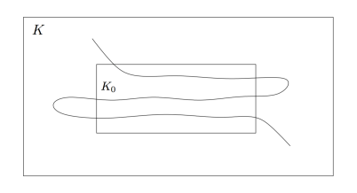
Figure 5: Compacts $K_{0}\subset K.$

By properness, we can take a compact cylinder $K_{0}\subset{\cal R}_{\epsilon}\cap\{t\geq t_{0}\}$ such that $X^{-1}\left(K_{0}\cap E\right)$ contains a finite number of connected components. Since any two of these connected components can be joined by a compact arc in $U$ and there are finitely many of those connected components, we can find a compact set $K\subset\{t\geq t_{0}\}$ containing $K_{0}$ so that any two points of $X^{-1}\left(K_{0}\cap E\right)$ can be joined by a curve contained in $X^{-1}\left(K\cap E\right)$ (see Figure 5). Moreover, if we take $K_{0}$ so that it contains $C_{\ell}\cap{\cal R}_{\epsilon}$, for some small annulus $C_{\ell}$, then every component of $M\cap\{t\geq t_{0}\}$ has a non empty intersection with $K_{0}$. If not, we can consider this annulus $C_{\ell}$ with $C_{\ell}\cap{\cal R}_{\epsilon}\subset K_{0}$ and $\partial C_{\ell}\cap R_{\epsilon}=\emptyset$. We could move isometrically $C_{\ell}$ keeping its boundary outside ${\cal R}_{\epsilon}$ to reach any point in ${\cal R}_{\epsilon}$. There will be a first point of contact with the component that does not meet $K_{0}$, a contradiction with the maximum principle. In particular we obtain:

Claim 2.

The number of vertical sheets of $M\cap\{t\geq t_{0}\}$ is finite.

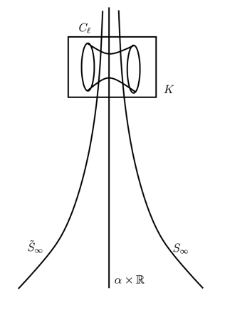
Figure 6: The slab, the compact $K$ and the annulus $C_{\ell}$.

We take $t_{1}>t_{0}$ such that $K$ is contained in the slab $\{t_{0}\leq t\leq t_{1}\}$ and let $t_{2}>t_{1}+2\rho$. Now let us consider $U^{\prime}$ a connected component of $X^{-1}\left(E\cap\{t>t_{2}\}\right)$, and $E^{\prime}=X(U^{\prime})$. Arguing as above we get that $U^{\prime}$ is simply-connected and $E^{\prime}$ is unbounded. And we can find two compact sets $K_{0}^{\prime},K^{\prime}$ contained in $\{t\geq t_{2}\}$ such that $K_{0}^{\prime}\cap E^{\prime}\neq\emptyset$ and any two points of $X^{-1}\left(K_{0}^{\prime}\cap E^{\prime}\right)$ can be joined by a curve in $X^{-1}\left(K^{\prime}\cap E^{\prime}\right)$. Let us consider $t_{3}$ such that $K^{\prime}$ is contained in the slab $\{t_{2}\leq t\leq t_{3}\}$ and take $t_{4}>t_{3}+2\rho$ (see Figure 7).

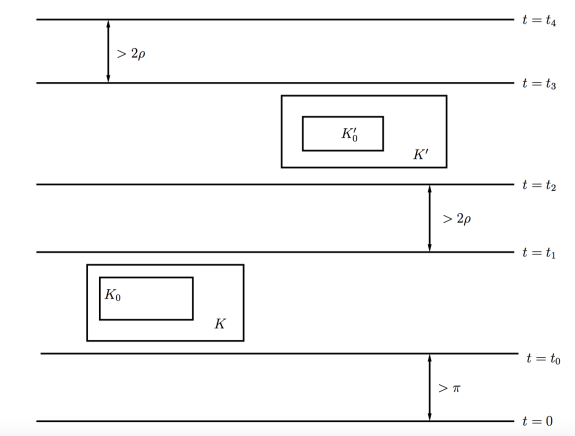
Figure 7: Compacts $K_{0}\subset K$ and $K^{\prime}_{0}\subset K^{\prime}$.

Consider $Y$ the unit vector field of $\operatorname{\mathbb{H}^{2}}$ normal to the foliation of $\operatorname{\mathbb{H}^{2}}$ by equidistant curves to $\alpha$ (and then tangent to the geodesics intersecting $\alpha$ orthogonally). This vector field $Y$ lifts to a horizontal field in $N^{3}$, also called $Y$.

Claim 3.

For $t^{\prime}>t_{4}$ large, $E^{\prime}\cap\{t>t^{\prime}\}$ is a horizontal geodesic graph over a domain of $\alpha\times\operatorname{\mathbb{R}}$, i.e., $E^{\prime}\cap\{t>t^{\prime}\}$ is transversal to the horizontal vector field $Y.$

Proof.

Take $T>0$ so that the annulus $A_{0}$ is contained in a horizontal slab $\{|t|Ê\leq T/2\}$. We prove Claim 3 for $t^{\prime}=T+t_{4}$. Suppose by contradiction that there exists a point $z\in U^{\prime}$ such that $q=X(z)\in\{t>T+t_{4}\})$ and $Y(q)\in T_{q}E^{\prime}.$

Choosing $\epsilon\leq\ell/2$ small enough, for any point $p\in A_{0}\cap(\gamma_{0}\times\operatorname{\mathbb{R}})$ there exists an isometry $\psi_{p}$ of $\operatorname{\mathbb{H}^{2}\times\mathbb{R}}$ such that $\psi_{p}(p)=q,$ $\psi_{p}(\partial A_{0})\cap{\cal R}_{\epsilon}=\emptyset$ and $\psi_{p}(\partial C_{\ell})\cap{\cal R}_{\epsilon}=\emptyset$. Hence, since the normal vector to $A_{0}$ along $A_{0}\cap(\gamma_{0}\times\operatorname{\mathbb{R}})$ takes all directions in the plane $\gamma_{0}\times\operatorname{\mathbb{R}}$, we can find a point $p_{0}\in A_{0}\cap(\gamma_{0}\times\operatorname{\mathbb{R}})$ such that $\psi_{p_{0}}(p_{0})=q,$ $\psi_{p_{0}}(\partial A_{0})\cap{\cal R}_{\epsilon}=\emptyset$ and $\psi_{p_{0}}(A_{0})$ is tangent to $E^{\prime}$ at $q.$ In order to simplify the notation, we still denote by $A_{0}$ the annulus $\psi_{p_{0}}(A_{0}),$ and by $P^{d}$ and $P^{-d}$ the vertical planes containing its boundary curves $\eta$ and $\eta_{-},$ respectively. We remark that $A_{0}$ is no more symmetric with respect to $\alpha\times\operatorname{\mathbb{R}}$ but we still denote by $\gamma_{0}\times\operatorname{\mathbb{R}}$ its plane of symmetry, so $q\in A_{0}\cap(\gamma_{0}\times\operatorname{\mathbb{R}})$. Finally, we remark that $A_{0}\subset\{t>t_{4}>t_{3}+2\rho\}$, since $q\in\{t>T+t_{4}\})$.

Since $A_{0}$ and $E^{\prime}$ are tangent at $q$, we have that $X^{-1}\left(A_{0}\cap E^{\prime}\right)$ consists, locally around $z$, of at least two curves passing through $z$ in an equiangular way. Since neither the boundary of $A_{0}$ intersects $E^{\prime}$ nor the boundary of $E^{\prime}$ intersects $A_{0}$ and $U^{\prime}$ is simply connected, we have that these curves bound at least two local connected components $D_{1}$ and $D_{2}$ in $U^{\prime}$. These local components $D_{1}$ and $D_{2}$ are in distinct components of $X^{-1}(E^{\prime}\cap A_{0}^{-})$. In fact, suppose this is not true, so we can find a path $\alpha_{0}$ in $U^{\prime}$ with $X(\alpha_{0})\subset A_{0}^{-}$, joining points $x\in D_{1}$ and $y\in D_{2}$. Now join $x$ to $y$ by a local path $\beta_{0}$ in $U^{\prime}$ going through $p$ with $\beta_{0}\subset A_{0}^{-}$ except at $p$. Let $\Gamma=\alpha_{0}\cup\beta_{0}$, we have $X(\Gamma)\subset A_{0}^{-}$. Since $U^{\prime}$ is simply connected, $\Gamma$ bounds a disk $D$ in $U^{\prime}$, but by construction $X(D)\cap A_{0}^{+}\neq\emptyset$, a contradiction with Lemma 5. Hence $D_{1}$ and $D_{2}$ are contained in two distinct components of $U^{\prime}\backslash X^{-1}(A_{0}\cap E^{\prime})$ such that $X(D_{1})$ and $X(D_{2})$ are contained in $E^{\prime}\cap A_{0}^{-}$ (see Figure 8).

We observe that $D_{1}$ and $D_{2}$ are disjoint in $U^{\prime}$, even if their images by $X$ intersect each other (as the surface $M$ is not necessarily embedded).

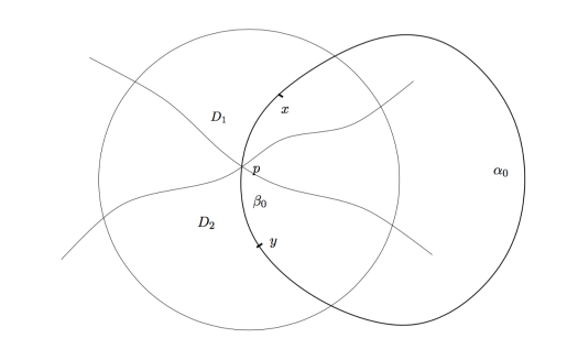
Figure 8: Components $D_{1}$ and $D_{2}$

Let $P$ be a vertical geodesic plane orthogonal to $\gamma_{0}\times\operatorname{\mathbb{R}}$ such that $P$ divides the intersection curve $A_{-\delta}\cap(\gamma_{0}\times\operatorname{\mathbb{R}})$ in two components. Denote by $P^{-}$ and $P^{+}$ the two halfspaces determined by $P$, and by $P^{-\rho},P^{\rho}$ the two equidistant planes to $P$ at a distance $2\rho$ from $P$. Let us denote by $[P^{-\rho},P^{\rho}]$ the slab bounded by $P^{-\rho}$ and $P^{\rho}$. We consider the ball $B_{0}=B_{q_{1}}(\rho)$ in $A_{0}^{-}$ of radius $\rho$ centered at the point $q_{1}$ of the “axis” $\xi$ of the annulus $A_{0}$ (see Section 2.3). This ball $B_{0}$ contains an annulus $C_{\ell_{0}}$ with boundary outside ${\cal R}_{\epsilon}.$ Notice that $B_{q_{1}}(2\rho)\cap\mbox{Tub}^{-}(A_{0})=\emptyset$ and then $B_{q_{1}}(4\rho)\subset A_{0}^{-}$. $B_{0}$ is contained in $[P^{-\rho},P^{\rho}]$ with its center at height $t=s_{0}$. For any $j=1,2$, we are going to prove that $X(D_{j})$ contains a point $z_{j}$ inside $C_{\ell_{0}}\subset B_{0}$. To see that we apply the maximum principle. We know that $X(D_{j})$ intersects each annulus $A_{s}$ in Tub${}^{-}(A_{0})$; then $X(D_{j})$ intersects a small annulus $C_{\ell_{j}}$ in Tub${}^{-}(A_{0})$ at a point $w_{j}$. By our choice of $\epsilon$, the boundary of $C_{\ell_{j}}$ does not intersect $X(D_{j})$ when translated in the direction of a vector in $\alpha\times\operatorname{\mathbb{R}}$. Using the Dragging Lemma with $D_{j}\subset U^{\prime}$ and translated copies of $C_{\ell_{j}}$, we find a curve in $X(D_{j})$ going from the point $w_{j}$ to a point $z_{j}\in C_{\ell_{0}}$, as desired. See Figure 9.

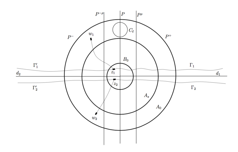
Figure 9: A vertical section of $A_{0},C_{\ell}$ and $[P^{-2\rho},P^{2\rho}].$

Using again the Dragging Lemma we consider horizontal translations of $C_{\ell_{0}},$ denoted by $C_{\ell}(t)$, along a horizontal geodesic in $P^{+},$ going very far from the slab $[P^{-\rho},P^{\rho}],$ and then going vertically downwards into the compact $K_{0}^{\prime}$ (applying as well horizontal translations, if needed, in order to get to the compact $K_{0}^{\prime}$ but with $\partial C_{\ell}(t)$ never touching the slab). Along this movement we follow a connected arc $\Gamma^{\prime}_{1}(t)\in U^{\prime}$ with $X(\Gamma^{\prime}_{1}(t))\in C_{\ell}(t)$ starting at $z_{1}$ and ending into $K_{0}^{\prime}$, with $X(\Gamma^{\prime}_{1})\cap A_{0}^{-}\subset X(D_{1})$. We denote by $\Gamma^{\prime}_{2}(t)\subset U^{\prime}$ a similar arc starting at $z_{2}$ and ending into $K_{0}^{\prime}$ with $X(\Gamma^{\prime}_{2})\cap A_{0}^{-}\subset X(D_{2})$. Notice we cannot connect $\Gamma^{\prime}_{1}$ and $\Gamma^{\prime}_{2}$ before they leave $A_{0}^{-}$ (since $D_{1}$ and $D_{2}$ are in two disjoint components). If they meet in $U^{\prime}$ before ending into $K_{0}^{\prime}$, we stop the construction at the first point of intersection. If not we connect $\Gamma^{\prime}_{1}$ and $\Gamma^{\prime}_{2}$ by an arc $\alpha^{\prime}$ contained in the compact set $X^{-1}(K^{\prime})$, since they have endpoint in $K_{0}^{\prime}$ (see Figure 9).

We apply the same construction in $P^{-}$. We move the annulus $C_{\ell}$ along first a horizontal geodesic into $P^{-}$, next we move the annulus vertically downwards (and horizontally, if necessary) to end into $K_{0}$. We construct an arc $\Gamma_{1}$ from $z_{1}$ to $K_{0}$ and an arc $\Gamma_{2}$ from $z_{2}$ into $K_{0}$. We connect eventually $\Gamma_{1}$ and $\Gamma_{2}$ by an arc $\alpha$ in $X^{-1}(K)$.

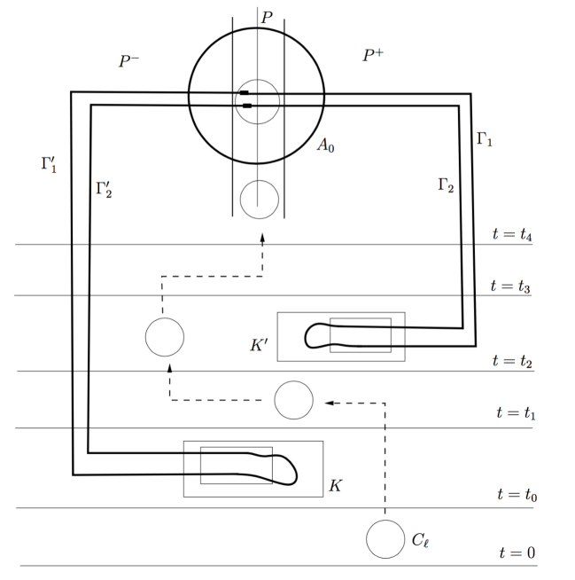
Figure 10: Curve $\widetilde{\Gamma}$.

Therefore $\widetilde{\Gamma}=\Gamma_{1}\cup\Gamma_{2}\cup\alpha\cup\Gamma^{\prime}_{1}\cup\Gamma_{2}^{\prime}\cap\alpha^{\prime}$ is a simple closed curve in $U$ (see Figure 10). We call $D$ the compact disk in $U$ bounded by $\widetilde{\Gamma}$. Now we consider a small annulus $C_{\ell}\subset\mbox{Tub}^{+}(A_{0})$ lying under $A_{0}$ and such that $C_{\ell}\cap P\neq\emptyset$. For instance, we can take $C_{\ell}$ contained in the ball of radius $\rho$ centered at a point in $P\cap A_{\delta/2}\cap(\gamma_{0}\times\operatorname{\mathbb{R}}).$

We move isometrically the small annulus $C_{\ell}$ to $\{t<t_{0}\}$ keeping its boundary outside ${\cal R}_{\epsilon}$. We consider a family of annuli obtained by continuously translating back $C_{\ell}$ from $\{t<t_{0}\}$ to its original position in $\mbox{Tub}^{+}(A_{0})\cap[P^{-\rho},P^{\rho}]$. By the choice of $\widetilde{\Gamma}$, we can assume that none of these translated annuli intersects $X(\widetilde{\Gamma})$ and then, by the maximum principle, they do not intersect the minimal disk $X(D)$ either (observe that $X(D)\subset{\cal R}_{\epsilon}$, so $X(D)$ cannot intersect the boundary of the annuli). Translating slightly $C_{\ell}$ inside $A_{0}^{-}$ and using the maximum principle, we get that $X(D)$ has no points in $P\cap\{t_{4}\leq t\leq s_{0}-3\rho\}.$ Using the maximum principle with the anulli $C_{\ell}$ coming from above $A_{0}$ and going downwards inside $A_{0}^{-}$ in the region $[P^{-\rho},P^{\rho}]\cap\{t\geq s_{0}+3\rho\},$ we also conclude that $X(D)$ has no points in $P\cap\{t\geq s_{0}+3\rho\}.$ Possibly slightly translating $P$, we can suppose that $X(D)\cap P$ is transversal.

Since $X(\Gamma_{1}\cup\Gamma_{1}^{\prime})$ is a curve which crosses $P$ transversally going from $P^{-}$ to $P^{+}$ then the number of points in $(\Gamma_{1}\cup\Gamma_{1}^{\prime})\cap X^{-1}(P)$ is odd. Now we consider a curve $\beta$ in $D\cap X^{-1}(P)$ starting at a point $p\in\Gamma_{1}\cup\Gamma_{1}^{\prime}$. We observe that by the maximum principle $\beta$ can not be a closed curve, so it does not finish at $p$. Since $X(D)$ does not intersect $P\cap(\{t_{4}\leq t\leq s_{0}-3\rho\}\cup\{t\geq s_{0}+3\rho\})$, we get that $\beta$ is contained in $X^{-1}(A_{0}^{-}\cap P).$ Hence $\beta$ is a curve entirely contained in the component $D_{1}$ and finishes at a different point in $\Gamma_{1}\cup\Gamma_{1}^{\prime}$ concluding that the number of points in the intersection $P\cap(\Gamma_{1}\cup\Gamma_{1}^{\prime})$ is even, a contradiction. Therefore, we conclude that $E^{\prime}\cap\{t\geq t^{\prime}=T+t_{4}\}$ is necessarily transversal to the horizontal vector field $Y.$ ∎

Let $t^{\prime}>T+t_{4}$, we call $\widetilde{U}$ a connected component of $X^{-1}(E^{\prime}\cap\{t>t^{\prime}\})$ and $\widetilde{E}=X(\widetilde{U}).$ We have proved that the horizontal sheet $\widetilde{E}$ is a horizontal geodesic graph over $\alpha\times\operatorname{\mathbb{R}}$ for some geodesic in the direction of the vector field $Y$.

Similarly, we can prove that for $t^{\prime}$ large, $X^{-1}(M\cap\{t<-t^{\prime}\})$ has a finite number of connected components $\tilde{V}$ and each $X(\tilde{V})$ is a horizontal graph over $\beta\times\operatorname{\mathbb{R}}$ for some geodesic $\beta$ such that $\beta\times\{-1\}\subset{\cal P}$.

Claim 4.

For $t^{\prime}>T+t_{4}$ large, $E^{\prime}\cap\{t>t^{\prime}\}$ (resp. $E^{\prime}\cap\{t<-t^{\prime}\}$) is a horizontal Killing graph over a domain of $\alpha\times\operatorname{\mathbb{R}}$ (resp. $\beta\times\operatorname{\mathbb{R}}$).

Proof.

We consider the half-space model of $\operatorname{\mathbb{H}^{2}}$ with orthonormal basis $(e_{1},e_{2})$ and the geodesic $\alpha$ represented by the half-line $\{x=0\}$. In this model the equidistant curves $\alpha^{-\epsilon}$ and $\alpha^{\epsilon}$ are half-lines making angles $\pm\theta$ with $\{x=0\}$. In this model, horizontal translations of the annulus $A_{0}$ (keeping the origin as a fixed point at infinity) correspond to homoteties and rotations centered at the origin of the model in such a way that the boundary curves of $A_{0}$ do not intersect $\alpha^{-\epsilon}\times\operatorname{\mathbb{R}}$ nor $\alpha^{\epsilon}\times\operatorname{\mathbb{R}}$. Claim 3 implies that we cannot find a point of $E$ which is tangent to $A_{0}$ along its symmetry curve $\gamma_{0}\times\operatorname{\mathbb{R}}$. Looking for the set of admissible transformations, Claim 3 concludes that $E$ is transverse to any geodesic orthogonal to $\alpha\times\operatorname{\mathbb{R}}$.

To prove that the component $E$ is a horizontal Killing field, it suffices to move the annulus $A_{0}$ with homothety and horizontal translation along $e_{1}$ direction and check that we can place $\gamma_{0}\times\operatorname{\mathbb{R}}$ in any position of the slab with boundary of $A_{0}$ not intersecting $\alpha^{-\epsilon}\times\operatorname{\mathbb{R}}$ and $\alpha^{\epsilon}\times\operatorname{\mathbb{R}}$. If we choose $\epsilon>0$ such that it is possible at height $y=1$ into the half-plane model, then we have the same degree of freedom at each $y>1$, using isometries of $\operatorname{\mathbb{H}^{2}}$. ∎

Let $\alpha\times\{1\}$ and $\beta\times\{-1\}$ be two geodesics in ${\cal P}$ such that $\alpha$ and $\beta$ share an endpoint $a\in\partial_{\infty}\operatorname{\mathbb{H}^{2}}$. We consider a foliation of horocylinders $\bigcup_{c\geq c_{0}}{\mathcal{H}}(c)$ with boundary points at infinity $\{a\}\times\operatorname{\mathbb{R}}$ and we consider a horizontal sheet $E$ of $M\cap\bigcup_{c\geq c_{0}}{\mathcal{H}}(c)$ parametrized by $X(U)$. Recall that $X(U)\subset\Omega\times\operatorname{\mathbb{R}}$ (see the beginning of Section 3). Let us denote by $\alpha_{1},\beta_{1}$ the geodesics in $\partial\Omega$. Let $\gamma_{c}$ be the geodesic orthogonal to $\alpha$ passing through the point $\alpha\cap{\mathcal{H}}(c)$. For $c$ large enough, $\beta_{1}\cap\gamma_{c}$ is non empty.

We consider the cusp end of $\Omega$ bounded by arcs $\tilde{\gamma}_{c_{0}},\tilde{\alpha}_{1}$ and $\tilde{\beta}_{1}$, contained in $\gamma_{c_{0}},\alpha_{1}$ and $\beta_{1}$. Consider $c_{0}$ sufficiently large so that the distance between $\gamma_{c_{0}}\cap\tilde{\alpha}_{1}$ and $\gamma_{c_{0}}\cap\tilde{\beta}_{1}$ is less than $\epsilon$ and $M\cap\bigcup_{c\geq c_{0}}{\mathcal{H}}(c)$ is contained in a vertical slab ${\cal R}_{\epsilon}$ of width $\epsilon$.

Let $Y$ be the vector field defined just before Claim 3 for $\alpha$.

Claim 5.

For $c^{\prime}$ large, any horizontal sheet in $M\cap\bigcup_{c\geq c_{0}}{\mathcal{H}}(c)$ is a horizontal geodesic graph over a domain of $\alpha\times\operatorname{\mathbb{R}}$ transverse to the field $Y$ and contained in ${\cal R}_{\epsilon}$.

Proof.

We take $c_{0}\in\operatorname{\mathbb{R}}$ large enough so that $\partial M\cap\left(\cup_{c\geq c_{0}}\gamma_{c}\times\operatorname{\mathbb{R}}\right)=\emptyset$. By the maximum principle using vertical geodesic planes, we know that no connected component of $M\cap(\gamma_{c_{0}}\times\operatorname{\mathbb{R}})$ can bound a compact disk in $M$.

We take an ideal geodesic quadrilateral ${\cal Q}\subset\operatorname{\mathbb{H}^{2}}$, two of whose opposite edges are $\gamma_{c_{0}}$ and $\gamma_{c_{1}}$, for some $c_{1}>c_{0}$, and such that there exists a Scherk minimal graph defined over ${\cal Q}$ with boundary values $+\infty$ over $\gamma_{c_{0}}\cup\gamma_{c_{1}}$ and $-\infty$ over the other two edges. Taking $c_{0}$ large enough, we can assume that $\partial{\cal Q}\setminus(\gamma_{c_{0}}\cup\gamma_{c_{1}})\subset\operatorname{\mathbb{H}^{2}}\setminus\Omega$ (recall that $M\subset\Omega\times\operatorname{\mathbb{R}}$).

We now claim that $M\cap(\gamma_{c}\times\operatorname{\mathbb{R}}),$ for $c>c_{1}$, does not contain any compact curve $\Gamma$. Suppose this was not the case. We already know that $\Gamma$ has to be in the homology class of $\partial M$. Thus $\Gamma\cup\partial M$ bounds an annulus $A$. Using the maximum principle with $A$ and vertically translated copies of the Scherk graph just described above, we reach a contradiction.

Given $c_{2}>c_{1}$, we consider a connected component $E=X(U)$, where $U$ is a connected component of $X^{-1}\left(M\cap(\cup_{c>c_{2}}\gamma_{c}\times\operatorname{\mathbb{R}})\right)$. We can assume that $(\gamma_{c_{2}}\times\operatorname{\mathbb{R}})\cap{\cal R}_{\epsilon}$ is transversal. We have proved that $U$ is simply-connected and $\partial E$ consists of curves joining $(\alpha\cap\gamma_{c_{2}})\times\{-1\}$ to $(\beta\cap\gamma_{c_{2}})\times\{1\}$ (possibly no one) and perhaps some curves whose endpoints are both in $(\beta\cap\gamma_{c_{2}})\times\{-1\}$ or $(\alpha\cap\gamma_{c_{2}})\times\{1\}$. We know that $X^{-1}(M\cap\{|t|>t^{\prime}\})$ has a finite number of connected components and each one of them corresponds to (via $X$) a horizontal graph. Hence we get that $\partial E$ has a finite number of curves.

Take a compact set $K_{0}$ contained in the halfspace $\cup_{c>c_{2}}(\gamma_{c}\times\operatorname{\mathbb{R}})$. By properness, there are a finite number of connected components in $X^{-1}(K_{0}\cap E)$. Hence we can find a compact set $K\subset\cup_{c>c_{2}}(\gamma_{c}\times\operatorname{\mathbb{R}})$ containing $K_{0}$ so that any two points of $X^{-1}(K_{0}\cap E)$ can be joined by a curve contained in $X^{-1}(K\cap E)$. Let us suppose that $K$ is contained in the vertical slab between $(\gamma_{c_{2}}\times\operatorname{\mathbb{R}})$ and $(\gamma_{c_{3}}\times\operatorname{\mathbb{R}}),$ for some $c_{3}>c_{2}.$

Now let us consider a connected component $E^{\prime}=X(U^{\prime})$, where $U^{\prime}$ is a connected component of $X^{-1}\left(E\cap(\cup_{\{c\geq c_{3}+2\rho\}}\gamma_{c}\times\operatorname{\mathbb{R}})\right),$ where $\rho$ is the radius of the extrinsic balls where the small annuli $C_{\ell}$ are contained in. We observe that the boundary of $\partial C_{\ell}$ is outside ${\cal R}_{\epsilon}$.

Analogously, we can find two compact sets $K^{\prime}_{0},K^{\prime}\subset\cup_{\{c\geq c_{3}+2\rho\}}\gamma_{c}\times\operatorname{\mathbb{R}}$ such that any two points of $X^{-1}(K^{\prime}_{0}\cap E^{\prime})$ can be joined by a curve in $X^{-1}(K^{\prime}\cap E^{\prime}).$ We take $c_{4}>c_{3}+2\rho$ such that $K^{\prime}$ is contained in the vertical slab between $\gamma_{c_{3}+2\rho}\times\operatorname{\mathbb{R}}$ and $\gamma_{c_{4}}\times\operatorname{\mathbb{R}}$.

Suppose that the annulus $A_{0}$ can be contained in $\cup_{\{0\leq r\leq c_{5}\}}(\gamma_{r}\times\operatorname{\mathbb{R}})$ and we take $c^{\prime}>c_{4}+c_{5}+2\rho$. Now we can argue verbatim to the proof of Claim 3 using this new $E^{\prime}$ contained in the slab ${\cal R}_{\epsilon}$ and the annuli $A_{0}$ and $C_{\ell}$ with boundaries outside ${\cal R}_{\epsilon}$. To do that it is enough to check that we can move $A_{0}$ and $C_{\ell}$ with boundary curves outside ${\cal R}_{\epsilon}$. In the model of the half-plane with $a$ at infinity, the curves $\tilde{\alpha}_{1}$ and $\tilde{\beta}_{1}$ are parallel vertical half-lines. The annuli can be moved using homothety and horizontal translations as in Claim 4.

These arguments show that $E^{\prime}\cap\cup_{c\geq c^{\prime}}(\gamma_{c}\times\operatorname{\mathbb{R}})$ is transversal to the vector field $Y$.

We call $\widetilde{U}$ a connected component of $X^{-1}\left(E^{\prime}\cap\cup_{\{c\geq c^{\prime}\}}(\gamma_{c}\times\operatorname{\mathbb{R}})\right)$ and $\widetilde{E}=X(\widetilde{U})$. Hence $\widetilde{E}$ is a horizontal geodesic and Killing graph. More precisely, for any $c>c^{\prime}$, $\widetilde{E}\cap(\gamma_{c}\times\operatorname{\mathbb{R}})$ consists of one curve $d_{c}=d_{c}(t)$ joining $(\beta\cap\gamma_{c^{\prime}})\times\{-1\}$ to $(\alpha\cap\gamma_{c^{\prime}})\times\{1\}$ and $\partial\widetilde{E}=d_{c^{\prime}}$.

∎

Claim 6.

A horizontal Killing graph asymptotic to an admissible polygonal has finite total curvature

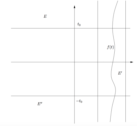
Figure 11: Domain $E\cup E^{\prime}\cup E^{\prime\prime}$

Proof.

In $\operatorname{\widetilde{\rm PSL}_{2}(\operatorname{\mathbb{R}},\tau)}$ this claim has been proved in [20] by constructing barrier to control the decay of the curvature $K$ on a Killing horizontal multigraph with finite number of sheets. Killing fields are used to get estimates of curvature by stability argument. The number of sheets is limited by the boundary at infinity of $M$ which is a polygonal line with finite number of edges and the fact that we assume that the immersion is proper.

In $\operatorname{\mathbb{H}^{2}}\times\operatorname{\mathbb{R}}$, we complete the proof by using conformal parametrization by its third coordinate. We consider a vertical sheet $E\subset M\cap\{t>t_{0}\}$ and we reparametrize conformally $E$ by $w=u+it$ on $\Omega_{0}=\{t\geq t_{0}\},$ where $t$ is the third coordinate of the conformal immersion in $\operatorname{\mathbb{H}^{2}}\times\operatorname{\mathbb{R}}$ (since $E$ is a horizontal graph, the tangent plane is never horizontal and $t$ is defined globally on $E$) given by

$$X(u,t)=(F(u,t),t)\in\operatorname{\mathbb{H}^{2}}\times\operatorname{\mathbb{R}}.$$

The quadratic Hopf differential associate with the horizontal harmonic map $F:\Omega\to\operatorname{\mathbb{H}^{2}}$ is given by $Q=\frac{1}{4}(dw)^{2}$ and the conformal metric of the conformal immersion is given by $ds^{2}=\cosh^{2}\omega|dw|^{2}$ with

$$|F_{u}|_{\operatorname{\mathbb{H}^{2}}}=\cosh^{2}\omega\hbox{ and }|F_{t}|_{\operatorname{\mathbb{H}^{2}}}=\sinh^{2}\omega.$$ (3.1)

In this parametrization $n_{3}=\tanh\omega$ is the third component of the normal (see Section 2.4). The decay estimate on $\omega$ providing $Q$ has no zeros on $E$ is given by

$$|\omega|(u,t)\leq C_{0}e^{-t},$$

where $C_{0}$ is a constant depending on $t_{1}$, for any $t\geq t_{1}>t_{0}$, $t_{1}$ large enough. We need to improve this decay in the variable $u$ to conclude finite total curvature.

Using barriers, $E$ is uniformly asymptotic to $\alpha\times\operatorname{\mathbb{R}}$ at infinity. Let $a\in\partial_{\infty}\alpha$ and consider $M\cap\{{\mathcal{H}}(c);c\geq c_{0}\}$ where $\partial_{\infty}{\mathcal{H}}(c)=\{a\}\times\operatorname{\mathbb{R}}$. There is a horizontal sheet $E^{\prime}\subset MÊ\cap\{{\mathcal{H}}(c);c\geq c_{0}\}$ which extends to $E$.

Since $E^{\prime}$ is a horizontal multigraph on $\alpha\times\operatorname{\mathbb{R}}$, $E^{\prime}$ can be conformally parametrized by some topological half-plane $\{w=u+it;u\geq f_{0}(t)\},$ where $f_{0}:\operatorname{\mathbb{R}}\to\operatorname{\mathbb{R}}$ is a continuous function. The curve $t\to X(f(t),t)$ is a parametrization of $\partial E^{\prime}\subset M\cap{\mathcal{H}}(c_{0})$ which extends $E$. For $t\leq-t_{0}$, $E^{\prime}$ is connected to a vertical sheet $E^{\prime\prime}\subset M\cap\{t\leq-t_{0}\}$.

We parametrize $E\cup E^{\prime}\cup E^{\prime\prime}$ globally on some domain $\Omega_{1}\subset\operatorname{\mathbb{C}}$ where the third coordinate is $x_{3}=t$ (see Figure 11). We study $t\to F(s,t)\subset\operatorname{\mathbb{H}^{2}}$, the immersion of the curve $\{u=s;t\in\operatorname{\mathbb{R}}\}$ for $s\geq\sup_{t\in[-t_{0},t_{0}]}f(t)$. Since $|\omega|(s,t)\leq C^{\prime}e^{-t}$, using (3.1), the curve $t\to F(s,t)$ is non proper and contained in a compact arc linking two points into consecutive geodesics $\alpha$ and $\beta$ of ${\mathcal{P}}$ having same infinite point $a\in\partial_{\infty}\operatorname{\mathbb{H}^{2}}$. When $s\to\infty$, the arc is uniformly diverging to infinity since the end $M$ is properly immersed. In particular, for $s$ large enough, the arc is contained in the convex domain bounded by ${\mathcal{H}}(c_{1})$ for some $c_{1}\geq c_{0}$. We observe that this argument implies that for any $c_{2}\geq c_{1}$, the curve $(E\cup E^{\prime}\cup E^{\prime\prime})\cap{\mathcal{H}}(c_{2})$ is parametrized in $\Omega$ by some curve $\{u=f_{2}(t)\}$ with $C_{1}\leq f_{2}(t)\leq C_{2}$.

This estimate provides a control of the boundary of horizontal sheet in the parametrization by the third coordinate on $\Omega_{1}$. Now we apply the decay estimate on $E^{\prime}$ and obtain that

$$|\omega|(u,t)\leq C_{1}e^{-u},$$

for $u>c_{3}$. This estimate holds on points of the vertical sheet $E$ for $u>c_{3}$ large enough close to the boundary point $a\in\partial_{\infty}\alpha$. We can do the same argument at the other boundary point of $\alpha$. Doing this we obtain a uniform decay on any vertical sheet $E$:

$$|\omega|(u,t)\leq C_{2}e^{-t-|u|},\hbox{ for }t\geq t_{1}>t_{0}\hbox{ and }u\in\operatorname{\mathbb{R}}.$$

Now using the fact that $\omega$ is solution of the elliptic equation $\Delta_{0}\omega-2|\phi|\sinh Ê\omega=0$, we apply interior gradient estimates to obtain that

$$|\omega|(u,t)+|\nabla\omega|(u,t)\leq C_{3}e^{-t-|u|},\hbox{ for }t\geq t_{1}>t_{0}\hbox{ and }u\in\operatorname{\mathbb{R}}.$$

This estimate provides finite total curvature for a vertical sheet $E$. The metric is $ds^{2}=Ê\cosh^{2}\omega|dz|^{2}$ and the curvature is given by

$$K(u,t)=-\tanh^{2}\omega-\frac{|\nabla\omega|^{2}}{4\cosh^{2}\omega}\leq 0.$$

Using the exponential decay this proves that any vertical sheet of $M\cap\{|t|\geq Êt_{1}\}$ has finite total curvature:

$$\int_{E\cap\{t\geq t_{1}\}Ê}|K|dAÊ\leq C.$$

It remains to study the horizontal sheets of $M$ in a slab which are connecting two vertical sheets as we describe above. We parametrize any horizontal sheet $E^{\prime}\subset M\cap\{|t|\leq 2t_{1}\}$ and we use the decay in the variable $u$ with variable $t$ bounded to obtain finite total curvature. Since the number of these sheets is bounded, the end $M$ has finite total curvature.

∎

For the next result we are going to use the following notion of length of a complete geodesic. Let $\Gamma$ be an ideal polygon with geodesics $\alpha_{i},\beta_{i}$. At each vertex $a_{i}$ of $\Gamma$ consider a horocycle $H_{i}$ so that $H_{i}\cap H_{j}=\emptyset$ if $i\neq j.$ Each geodesic $\alpha_{i}$ meets two of these horocycles, we denote by $|\alpha_{i}|$ the distance between them. We define $|\beta_{i}|$ in the same way. It is easy to see that $\sum_{i=1}^{k}|\alpha_{i}|-\sum_{i=1}^{k}|\beta_{i}|$ does not depend on the choice of the disjoint horocycles.

As corollaries of Theorem 9 we obtain the following theorems.

Theorem 12.

Let $M$ be a properly embedded minimal disk in $\operatorname{\mathbb{H}^{2}\times\mathbb{R}}$ asymptotic to an admissible polygon at infinity ${\cal P}$. Suppose that the vertical projection of ${\cal P}$ in $\operatorname{\mathbb{H}^{2}}$ is the boundary of a convex domain $\Omega$. Then $M$ is a vertical graph.

In particular, if $\alpha_{i}\times\{1\}$ and $\beta_{i}\times\{-1\}$, with $i=1,\dots,k$, are the edges of ${\cal P}$ then:

1. $\sum_{i=1}^{k}|\alpha_{i}|=\sum_{i=1}^{k}|\beta_{i}|$; and

2. for any inscribed polygonal domain $D$ in $\Omega$, $\sum_{i=1}^{k}|\alpha_{i}\cap\partial D|=\sum_{i=1}^{k}|\beta_{i}\cap\partial D|$,

where $|\bullet|$ denotes the hyperbolic length of the curve $\bullet$ as above.

Proof.

We first observe that, using the maximum principle with vertical geodesic planes, we get that $M\subset\Omega\times\operatorname{\mathbb{R}}$.

By Claims 2 and 3, there exists $t^{\prime}\in\operatorname{\mathbb{R}}$ such that $M\cap\{t>t^{\prime}\}$ has a finite number of connected components (we are using that $M$ is embedded), being each one of them a horizontal geodesic graph over the plane defined by a horizontal geodesic in ${\cal P}$. Let $E$ be one such component that is a horizontal geodesic graph over a domain of $\alpha\times\operatorname{\mathbb{R}}$, where $\alpha\times\{1\}\subset{\cal P}$. We call $E^{*}$ the reflected copy of $E$ with respect to $\{t=t^{\prime}\}$.

Let $\Delta$ be the component of $\operatorname{\mathbb{H}^{2}}-\alpha$ such that $\Delta\cap\Omega=\emptyset$, and fix a point $p_{\infty}\in\partial_{\infty}\Delta-\overline{\alpha}$. We take a geodesic $\gamma$ orthogonal to $\alpha$ with $p_{\infty}$ as one of its endpoints. We can consider a horizontal translation of $E^{*}$ along $\gamma$ towards $p_{\infty}\times\operatorname{\mathbb{R}}$ so that it does not intersect $M$. We translate back $E^{*}$ until reaching its original position. By the maximum principle, none of these translated copies of $E^{*}$ can intersect $M$.

Up to a vertical translation, we can assume $t^{\prime}=0$. We denote $M_{s}=M\cap\{t<-s\}$ and $M_{s}^{*}$ the reflected copy of $M-\overline{M_{s}}$ with respect to $\{t=-s\}$. We have proved that $M_{0}$ and $M_{0}^{*}$ are disjoint. We can then start applying Alexandrov Reflection Principle, and we obtain that $M_{s}$ and $M_{s}^{*}$ are disjoint for any $s>0$. Since $t^{\prime}$ could be taken arbitrarily large, we conclude that $M$ is a vertical graph.

Since $M$ is a vertical graph assuming $+\infty$ on $\alpha_{i}$ and $-\infty$ on $\beta_{i},$ we know that it has to be a Jenkins-Serrin-type graph. In particular, by Collin and Rosenberg [5] the length of the geodesic arcs on the ideal polygon must satisfy the conditions described on the statement of this theorem.

∎

Theorem 13.

Let $M$ be a properly embedded minimal surface in $\operatorname{\mathbb{H}^{2}\times\mathbb{R}}$ asymptotic to a finite number of vertical geodesic planes $\alpha_{i}\times\operatorname{\mathbb{R}}$, $i=1,\dots,k$, cyclically ordered (i.e. there exists an ideal convex polygonal domain $\Omega\subset\operatorname{\mathbb{H}^{2}}$ whose vertices - all of them at infinity - are the endpoints of the geodesics $\alpha_{i}$.) Then $M$ is a vertical bigraph symmetric with respect to a horizontal slice.

Proof.

We proceed as in the proof of the previous theorem and obtain that $M_{0}$ and $M_{0}^{*}$ are disjoint. More precisely, if ${\cal M}$ denotes the component of $\operatorname{\mathbb{H}^{2}\times\mathbb{R}}-M$ containing $\Delta\times\operatorname{\mathbb{R}}$, then $M_{0}^{*}$ is contained in ${\cal M}$. Applying Alexandrov Reflection Principle we get that $M_{s}^{*}\subset{\cal M}$ for $s$ small. But there must exist $s_{0}>0$ such that $M_{s_{0}}^{*}=M_{s_{0}}$ because otherwise we would reach a contradiction. Hence $M$ is symmetric with restect to $\{t=s_{0}\}$. ∎

References

- [1] P. Collin, L. Hauswirth and M. Hoang Nguyen, Construction of Minimal annuli in via variational method, preprint.
- [2] P. Collin, L. Hauswirth and H. Rosenberg, Properly immersed minimal surfaces in a slab of the hyperbolic plane, Archiv Math., 104 (2015), 471–484.
- [3] P. Collin, L. Hauswirth and H. Rosenberg, Properly immersed minimal surfaces in a slab of the hyperbolic plane, Archiv Math., 104 (2015), 471–484.
- [4] P. Collin, L. Hauswirth and H. Rosenberg, Minimal surfaces in finite volume hyperbolic 3-manifolds and in a finite area hyperbolic surface, preprint, arXiv:1304.1773v1.
- [5] P. Collin and H. Rosenberg, Construction of harmonic diffeomorphisms and minimal graphs, Ann. of Math., 172 (2010), 1879–1906.
- [6] B. Daniel. Isometric immersions into and and applications to minimal surfaces, Trans. A.M.S., 361 (2009), 6255–6282.
- [7] R. Sa Earp and E. Toubiana, A minimal stable vertical planar end in has finite total curvature,. arXiv:1310.5679.
- [8] R. Sa Earp and E. Toubiana, Concentration of total curvature of minimal surfaces in ,arXiv:1603.03335.
- [9] D. Fischer-Colbie and R. Schoen, The structure of complete stable minimal surfaces in 3-manifolds of non-negative scalar curvature, Comm. Pure Appl. Math., 33 (1980), 199–211.
- [10] A. Folha and C. Peñafiel, Minimal graphs in , preprint.
- [11] L. Hauswirth, Minimal surfaces of Riemann type in three-dimensional product manifolds, Pacific J. Math., 224 (2006), 91–117.
- [12] L. Hauswirth, B. Nelli, R. Sa Earp and E. Toubiana, Minimal ends in with finite total curvature and a Schoen type theorem, Advances in Mathematics, 274 (2015), 199–240.
- [13] L. Hauswirth and H. Rosenberg, Minimal surfaces of finite total curvature in , Mat. Contemp., 31 (2006), 65–80 .
- [14] F. Martín, R. Mazzeo and M.M. Rodríguez, Minimal surfaces with positive genus and finite total curvature in , Geometry and Topology, 18 (2014), 141–177.
- [15] L. Mazet, M.M. Rodríguez and H. Rosenberg, The Dirichlet problem for the minimal surface equation with possible infinite boundary data over domains in a Riemannian surface, Proc. London Math. Soc., 102 (2011), 985–1023.
- [16] L. Mazet, M. Magdalena Rodríguez and H. Rosenberg, Periodic constant mean curvature surfaces in , Asian J. Math., 18 (2014), 829–858.
- [17] S. Melo, Minimal graphs in over unbounded domains, Bull. Braz. Math. Soc., New Series, 45 (2014), 91–116.
- [18] F. Morabito and M.M. Rodríguez, Saddle towers and minimal -noids in , J. Inst. Math. Jussieu, 11 (2012), 333–349.
- [19] C. Penafiel, Invariant surfaces in and applications, Bull Braz Math. Soc., New Series, 43 (2012), 545-578.
- [20] M. Nguyen On existence of surfaces with finite total curvature in , preprint.
- [21] J. Pyo, New complete embedded minimal surfaces in , Ann. Glob. Anal. Geom., 40 (2011), 167–176.
- [22] J. Pyo and M.M. Rodríguez, Simply-connected minimal surfaces with finite total curvature in , Int. Math. Res. Notices, 2014 (2014), 2944-2954.
- [23] M.M. Rodríguez and G. Tinaglia, Non-proper complete minimal surfaces embedded in , Int. Math. Res. Not., 2015 (2015): 4322–4334.
- [24] H. Rosenberg, R. Souam and E. Toubiana, General curvature estimates for stable -surfaces in 3-manifolds and aplications, J. Dif. Geom., 84 (2010), 623–648.
- [25] R. Sa Earp and E. Toubiana, Screw motion surfaces in and , Illinois J. Math., 49 (2005), 1323–1362.
- [26] R. Schoen, Estimates for stable minimal surface in three dimensional manifolds, Ann. of Math. Studies, 103 (1983), 127–146.
- [27] R. Younes, Minimal surfaces in , Illinois J. Math., 54 (2010), no. 2, 671–712.