Stochastic Variance-Reduced ADMM

Abstract

The alternating direction method of multipliers (ADMM) is a powerful optimization solver in machine learning. Recently, stochastic ADMM has been integrated with variance reduction methods for stochastic gradient, leading to SAG-ADMM and SDCA-ADMM that have fast convergence rates and low iteration complexities. However, their space requirements can still be high. In this paper, we propose an integration of ADMM with the method of stochastic variance reduced gradient (SVRG). Unlike another recent integration attempt called SCAS-ADMM, the proposed algorithm retains the fast convergence benefits of SAG-ADMM and SDCA-ADMM, but is more advantageous in that its storage requirement is very low, even independent of the sample size $n$. We also extend the proposed method for nonconvex problems, and obtain a convergence rate of $O(1/T)$. Experimental results demonstrate that it is as fast as SAG-ADMM and SDCA-ADMM, much faster than SCAS-ADMM, and can be used on much bigger data sets.

I Introduction

In this big data era, tons of information are generated every day. Thus, efficient optimization tools are needed to solve the resultant large-scale machine learning problems. In particular, the well-known stochastic gradient descent (SGD) [1] and its variants [2] have drawn a lot of interest. Instead of visiting all the training samples in each iteration, the gradient is computed by using one sample or a small mini-batch of samples. The per-iteration complexity is then reduced from $O(n)$, where $n$ is the number of training samples, to $O(1)$. Despite its scalability, the stochastic gradient is much noisier than the batch gradient. Thus, the stepsize has to be decreased gradually as stochastic learning proceeds, leading to slower convergence.

Recently, a number of fast algorithms have been developed that try to reduce the variance of stochastic gradients [3, 4, 5, 6]. With the variance reduced, a larger constant stepsize can be used. Consequently, much faster convergence, even matching that of its batch counterpart, is attained. A prominent example is the stochastic average gradient (SAG) [5], which reuses the old stochastic gradients computed in previous iterations. A related method is stochastic dual coordinate ascent (SDCA) [6], which performs stochastic coordinate ascent on the dual. However, a caveat of SAG is that storing the old gradients takes $O(nd)$ space, where $d$ is the dimensionality of the model parameter. Similarly, SDCA requires storage of the dual variables, which scales as $O(n)$. Thus, they can be expensive in applications with large $n$ (big sample size) and/or large $d$ (high dimensionality).

Moreover, many machine learning problems, such as graph-guided fused lasso and overlapping group lasso, are too complicated for SGD-based methods. The alternating direction method of multipliers (ADMM) has been recently advocated as an efficient optimization tool for a wider variety of models [7]. Stochastic ADMM extensions have also been proposed [8, 9, 10], though they only have suboptimal convergence rates. Recently, researchers have borrowed variance reduction techniques into ADMM. The resultant algorithms, SAG-ADMM [11] and SDCA-ADMM [12], have fast convergence rate as batch ADMM but are much more scalable. The downside is that they also inherit the drawbacks of SAG and SDCA. In particular, SAG-ADMM and SDCA-ADMM require $O(nd)$ and $O(n)$ space, respectively, to store the past gradients and weights or dual variables. This can be problematic in large multitask learning, where the space complexities is scaled by $N$, the number of tasks. For example, in one of our multitask learning experiments, SAG-ADMM needs $38.2$TB for storing the weights, and SDCA-ADMM needs $9.6$GB for the dual variables.

To alleviate this problem, one can integrate ADMM with another popular variance reduction method, namely, stochastic variance reduced gradient (SVRG) [4]. In particular, SVRG is advantageous in that no extra space for the intermediate gradients or dual variables is needed. However, this integration is not straightforward. A recent initial attempt is made in [13]. Essentially, their SCAS-ADMM algorithm uses SVRG as an inexact stochastic solver for one of the ADMM subproblems. The other ADMM variables are not updated until that subproblem has been approximately solved. Analogous to the difference between Jacobi iteration and Gauss-Seidel iteration, this slows down convergence. Indeed, on strongly convex problems, SCAS-ADMM only has sublinear convergence while SDCA-ADMM has a linear rate. On general convex problems, SCAS-ADMM requires the stepsize to be gradually reduced. This defeats the original purpose of using SVRG-based algorithms, which aim at using a larger, constant learning rate to achieve fast convergence [4].

Besides, in spite of successful applications of ADMM to convex problems, the theoretical properties for nonconvex ADMM is not well understood and have been established very recently. In general, ADMM may fail to converge due to nonconvexity. However, it is found that ADMM has presented very good performance on many nonconvex problems. Indeed, the successful nonconvex applications includes matrix completion [14], tensor factorization [15] and robust tensor PCA [16]. Recently, Hong et al. [17] studied the convergence of the ADMM for solving certain nonconvex consensus and sharing problems, and showed that the generated sequence will converge to a stationary point, as well as a convergence rate of $O(1/T)$ for consensus problems, which underlines the feasibility of ADMM applications in nonconvex settings. Li and Pong [18] studied the convergence of ADMM for some special nonconvex composite models, and demonstrated that a stationary point of the nonconvex problem is guaranteed if the penalty parameter is chosen sufficiently large and the sequence generated has a cluster point. The Bregman multi-block ADMM, an extension of classic ADMM, has also been studied for a large family of nonconvex functions in [19]. Very recently, Wang et al. [20] also obtained convergence guarantee of ADMM on minimizing a class of nonsmooth nonconvex functions. The developed theoretical analysis includes various nonconvex functions such as piecewise linear function, the $\ell_{q}$ quasi-norm for $q\in(0,1)$ and Schatten-q quasi-norm ($0<q<1$), as well as the indicator functions of compact smooth manifolds. However, there is no known study for stochastic ADMM on nonconvex problems.

In this paper, we propose a tighter integration of SVRG and ADMM with a constant learning rate. The per-iteration computational cost of the resultant SVRG-ADMM algorithm is as low as existing stochastic ADMM methods, but yet it admits fast linear convergence on strongly convex problems. Among existing stochastic ADMM algorithms, a similar linear convergence result is only proved in SDCA-ADMM for a special ADMM setting. Besides, it is well-known that the penalty parameter in ADMM can significantly affect convergence [21]. While its effect on the batch ADMM has been well-studied [22, 21], that on stochastic ADMM is still unclear. We show that its optimal setting is, interestingly, the same as that in the batch setting. Moreover, SVRG-ADMM does not need to store the gradients or dual variables throughout the iterations. This makes it particularly appealing when both the number of samples and label classes are large. In addition, we also study the convergence properties of the proposed method for nonconvex problems, and obtain a convergence rate of $O(1/T)$ to a stationary point.

Notation: For a vector $x$, $\|x\|$ is its $\ell_{2}$-norm, and $\|x\|_{Q}=\sqrt{x^{T}Qx}$. For a matrix $X$, $\|X\|$ is its spectral norm, $\sigma_{\max}(X)$ (resp. $\sigma_{\min}(X)$) is its largest (resp. smallest) eigenvalue, and $X^{\dagger}$ its pseudoinverse. For a function $f$, $f^{\prime}$ is a subgradient. When $f$ is differentiable, we use $\nabla f$ as its gradient.

II Related Work

Consider the regularized risk minimization problem: $\min_{x}\frac{1}{n}\sum_{i=1}^{n}f_{i}(x)+r(x)$, where $x$ is the model parameter, $n$ is the number of training samples, $f_{i}$ is the loss due to sample $i$, and $r$ is a regularizer. For many structured sparsity regularizers, $r(x)$ is of the form $g(Ax)$, where $A$ is a matrix [23, 24]. By introducing an additional $y$, the problem can be rewritten as

$$\min_{x,y}\;f(x)+g(y)\;:\;Ax-y=0,$$ (1)

where

$$f(x)=\frac{1}{n}\sum_{i=1}^{n}f_{i}(x).$$ (2)

Problem (1) can be conveniently solved by the alternating direction method of multipliers (ADMM) [7]. In general, ADMM considers problems of the form

$$\min_{x,y}\;f(x)+g(y)\;:\;Ax+By=c,$$ (3)

where $f,g$ are convex functions, and $A,B$ (resp. $c$) are constant matrices (resp. vector). Let $\rho>0$ be a penalty parameter, and $u$ be the dual variable. At iteration $t$, ADMM performs the updates:

$$y_{t}\!\!\! = \!\!\!\arg\min_{y}g(y)+\frac{\rho}{2}\|Ax_{t-1}+By-c+u_{t-1}\|^{2},$$ (4)

$$x_{t}\!\!\! = \!\!\!\arg\min_{x}f(x)+\frac{\rho}{2}\|Ax+By_{t}-c+u_{t-1}\|^{2},$$ (5)

$$u_{t}\!\!\! = \!\!\!u_{t-1}+Ax_{t}+By_{t}-c.$$ (6)

With $f$ in (2), solving (5) can be computationally expensive when the data set is large. Recently, a number of stochastic and online variants of ADMM have been developed [10, 8, 9]. However, they converge much slower than the batch ADMM, namely, $O(1/\sqrt{T})$ vs $O(1/T)$ for convex problems, and $O(\log T/T)$ vs linear convergence for strongly convex problems.

For gradient descent, a similar gap in convergence rates between the stochastic and batch algorithms is well-known [5]. As noted by [4], the underlying reason is that SGD has to control the gradient’s variance by gradually reducing its stepsize $\eta$. Recently, by observing that the training set is always finite in practice, a number of variance reduction techniques have been developed that allow the use of a constant stepsize, and consequently faster convergence. In this paper, we focus on the SVRG [4], which is advantageous in that no extra space for the intermediate gradients or dual variables is needed. The algorithm proceeds in stages. At the beginning of each stage, the gradient $\tilde{z}=\frac{1}{n}\sum_{i=1}^{n}\nabla f_{i}(\tilde{x})$ is computed using a past parameter estimate $\tilde{x}$. For each subsequent iteration $t$ in this stage, the approximate gradient

$$\hat{\nabla}f(x_{t-1})=\frac{1}{b}\sum_{i_{t}\in\mathcal{I}_{t}}(\nabla f_{i_{t}}(x_{t-1})-\nabla f_{i_{t}}(\tilde{x}))+\tilde{z}$$ (7)

is used, where $\mathcal{I}_{t}$ is a mini-batch of size $b$ from $\{1,2,\dots,n\}$. Note that $\hat{\nabla}f(x_{t-1})$ is unbiased (i.e., $\mathbb{E}\hat{\nabla}f(x_{t-1})=\nabla f(x_{t-1})$), and its (expected) variance goes to zero asymptotically.

Recently, variance reduction has also been incorporated into stochastic ADMM. For example, SAG-ADMM [11] is based on SAG [5]; and SDCA-ADMM [12] is based on SDCA [6]. Both enjoy low iteration complexities and fast convergence. However, SAG-ADMM requires $O(nd)$ space for the old gradients and weights, where $d$ is the dimensionality of $x$. As for SDCA-ADMM, even though its space requirement is lower, it is still proportional to $N$, the number of labels in a multiclass/multilabel/multitask learning problem. As $N$ can easily be in the thousands or even millions (e.g., Flickr has more than 20 millions tags), SAG-ADMM and SDCA-ADMM can still be problematic.

III Integrating SVRG with Stochastic ADMM

In this paper, we make the following assumptions on the $f_{i}$’s in (2) and $g$ in (3).

Assumption 1.

Each $f_{i}$ is convex, continuously differentiable, and has $L_{i}$-Lipschitz-continuous gradient.

Hence, for each $i=1,\dots,n$, there exists $L_{i}>0$ such that

$$f_{i}(x_{j})\leq f_{i}(x_{i})+\nabla f_{i}(x_{i})^{T}(x_{j}-x_{i})+\frac{L_{i}}{2}\|x_{i}-x_{j}\|^{2},\forall x_{i},x_{j}$$

Moreover, Assumption 1 implies that $f$ is also smooth, with

$$f(x_{j})\leq f(x_{i})+\nabla f(x_{i})^{T}(x_{j}-x_{i})+\frac{L_{f}}{2}\|x_{i}-x_{j}\|^{2},$$

where $L_{f}\leq\frac{1}{n}\sum_{i=1}^{n}L_{i}\leq\max_{i}L_{i}$. Let $L_{\max}=\max_{i}L_{i}$. We thus also have

$$f(x_{j})\leq f(x_{i})+\nabla f(x_{i})^{T}(x_{j}-x_{i})+\frac{L_{\max}}{2}\|x_{i}-x_{j}\|^{2}.$$

Assumption 2.

$g$ is convex, but can be nonsmooth.

Let $(x_{*},y_{*})$ be the optimal (primal) solution of (3), and $u_{*}$ the corresponding dual solution. At optimality, we have

$$\nabla f(x_{*})+\rho A^{T}u_{*}=0,\;\;g^{\prime}(y_{*})+\rho B^{T}u_{*}=0,$$ (8)

$$Ax_{*}+By_{*}=c.$$ (9)

III-A Strongly Convex Problems

In this section, we consider the case where $f$ is strongly convex. A popular example in machine learning is the square loss.

Assumption 3.

$f$ is strongly convex, i.e., there exists $\lambda_{f}>0$ such that $f(x_{i})\geq f(x_{j})+\nabla f(x_{j})^{T}(x_{i}-x_{j})+\frac{\lambda_{f}}{2}\|x_{i}-x_{j}\|^{2}$ for all $x_{i},x_{j}$.

Moreover, we assume that matrix $A$ has full row rank. This assumption has been commonly used in the convergence analysis of ADMM algorithms [22, 25, 26, 21].

Assumption 4.

Matrix $A$ has full row rank.

The proposed procedure is shown in Algorithm 1. Similar to SVRG, it is divided into stages, each with $m$ iterations. The updates for $y_{t}$ and $u_{t}$ are the same as batch ADMM ((4) and (6)). The key change is on the more expensive $x_{t}$ update. We first replace (5) by its first-order approximation $f(x_{t-1})+\nabla f(x_{t-1})^{T}x$. As in SVRG, the full gradient $\nabla f(x_{t-1})$ is approximated by $\hat{\nabla}f(x_{t-1})$ in (7). Recall that $\hat{\nabla}f(x_{t-1})$ is unbiased and its (expected) variance goes to zero. In other words, $\hat{\nabla}f(x_{t-1})\rightarrow\nabla f(x_{*})$ when $x_{t-1}$ and $\tilde{x}$ approach the optimal $x_{*}$, which allows the use of a constant stepsize. In contrast, traditional stochastic approximations such as OPG-ADMM [9] use $\frac{1}{b}\sum_{i_{t}\in\mathcal{I}_{t}}\nabla f_{i_{t}}(x_{t-1})$ to approximate the full gradient, and a decreasing step size is needed to ensure convergence.

Unlike SVRG, the optimization subproblem in Step 9 has the additional terms $\frac{\rho}{2}\|Ax+By_{t}-c+u_{t-1}\|^{2}$ (from subproblem (5)) and $\frac{1}{2\eta}\|x-x_{t-1}\|_{G}^{2}$ (to ensure that the next iterate is close to the current iterate $x_{t-1}$). A common setting for $G$ is simply $G=I$ [8]. Step 9 then reduces to

$$x_{t}\!\!\!\!\! = \!\!\!\!\!\left(\frac{1}{\eta}I+\rho A^{T}A\right)^{-1}$$ (10)

$$\!\!\!\!\!\left(\frac{x_{t-1}}{\eta}\!\!-\!\!\hat{\nabla}f(x_{t-1})+\rho A^{T}(By_{t}-c+u_{t-1})\right).$$

Note that $(\frac{1}{\eta}I+\rho A^{T}A)^{-1}$ above can be pre-computed. On the other hand, while some stochastic ADMM algorithms [8, 11] also need to compute a similar matrix inverse, their $\eta$’s change with iterations and so cannot be pre-computed.

When $A^{T}A$ is large, storage of this matrix may still be problematic. To alleviate this, a common approach is linearization (also called the inexact Uzawa method) [27]. It sets $G=\gamma I-\eta\rho A^{T}A$ with

$$\gamma\geq\gamma_{\min}\equiv\eta\rho\|A^{T}A\|+1$$ (11)

to ensure that $G\succeq I$. The $x_{t}$ update in (10) then simplifies to

$$x_{t} = x_{t-1}-\frac{\eta}{\gamma}\left(\hat{\nabla}f(x_{t-1})\right.$$ (12)

$$\left.+\rho A^{T}(Ax_{t-1}+By_{t}-c+u_{t-1})\right).$$

Algorithm 1 SVRG-ADMM for strongly convex problems.

1:  Input: $m,\eta,\rho>0.$

2:  initialize $\tilde{x}_{0},\tilde{y}_{0}$ and $\tilde{u}_{0}=-\frac{1}{\rho}(A^{T})^{\dagger}\nabla f(\tilde{x}_{0})$;

3:  for $s=1,2,\dots$ do

4:     $\tilde{x}=\tilde{x}_{s-1}$;

5:     $x_{0}=\tilde{x}_{s-1}$; $y_{0}=\tilde{y}_{s-1}$; $u_{0}=\tilde{u}_{s-1}$;

6:     $\tilde{z}=\frac{1}{n}\sum_{i=1}^{n}\nabla f_{i}(\tilde{x})$;

7:     for $t=1,2,\dots,m$ do

8:        $y_{t}\leftarrow\arg\min_{y}g(y)+\frac{\rho}{2}\|Ax_{t-1}+By-c+u_{t-1}\|^{2}$;

9:        $x_{t}\leftarrow\arg\min_{x}\hat{\nabla}f(x_{t-1})^{T}x+\frac{\rho}{2}\|Ax+By_{t}-c+u_{t-1}\|^{2}+\frac{\|x-x_{t-1}\|^{2}_{G}}{2\eta}$;

10:        $u_{t}\leftarrow u_{t-1}+Ax_{t}+By_{t}-c$;

11:     end for

12:     $\tilde{x}_{s}=\frac{1}{m}\sum^{m}_{t=1}x_{t}$; $\tilde{y}_{s}=\frac{1}{m}\sum^{m}_{t=1}y_{t}$; $\tilde{u}_{s}=-\frac{1}{\rho}(A^{T})^{\dagger}\nabla f(\tilde{x}_{s})$;

13:  end for

14:  Output: $\tilde{x}_{s},\tilde{y}_{s}$;

Note that steps 2 and 12 in Algorithm 1 involve the pseudo-inverse $A^{\dagger}$. As $A$ is often sparse, this can be efficiently computed by the Lanczos algorithm [28].

In general, as in other stochastic algorithms, the stochastic gradient is computed based on a mini-batch of size $b$. The following Proposition shows that the variance can be progressively reduced. Note that this and other results in this section also hold for the batch mode, in which the whole data set is used in each iteration (i.e., $b=n$).

Proposition 1.

The variance of $\hat{\nabla}f(x_{t-1})$ is bounded by $\mathbb{E}\|\hat{\nabla}f(x_{t-1})-\nabla f(x_{t-1})\|^{2}\leq 4L_{\max}\beta(b)\left(J(x_{t-1})-J(x_{*})+J(\tilde{x})-J(x_{*})\right)$, where $L_{\max}\equiv\max_{i}L_{i}$, $\beta(b)=\frac{n-b}{b(n-1)}$, $J(x)=f(x)+\rho u_{*}^{T}Ax$, and $J(x_{t-1})-J(x_{*})+J(\tilde{x})-J(x_{*})\geq 0$.

Using (8) and (9), $J(x)-J(x_{*})=f(x)-f(x_{*})-\nabla f(x_{*})^{T}(x-x_{*})=0$ when $x\rightarrow x_{*}$, and thus the variance goes to zero. Moreover, as expected, the variance reduces when $b$ increases, and goes to zero when $b=n$. However, a large $b$ leads to a high per-iteration cost. Thus, there is a tradeoff between “high variance with cheap iterations” and “low variance with expensive iterations”.

III-A1 Convergence Analysis

In this section, we study the convergence w.r.t. $R(x,y)\equiv f(x)-f(x_{*})-\nabla f(x_{*})^{T}(x-x_{*})+g(y)-g(y_{*})-g^{\prime}(y_{*})^{T}(y-y_{*})$. First, note that $R(x,y)$ is always non-negative.

Proposition 2.

$R(x,y)\geq 0$ for any $x$ and $y$.

Using the optimality conditions in (8) and (9), $R(x,y)$ can be rewritten as $f(x)+g(y)+\rho u_{*}^{T}(Ax+By-c)-(f(x_{*})+g(y_{*})+\rho u_{*}^{T}(Ax_{*}+By_{*}-c))$, which is the difference of the Lagrangians in (3) evaluated at $(x,y,u_{*})$ and $(x_{*},y_{*},u_{*})$. Moreover, $R(x,y)\geq 0$ is the same as the variational inequality used in [29].

The following shows that Algorithm 1 converges linearly.

Theorem 1.

Let

$$\kappa\! \!=\! \!\frac{\|G+\eta\rho A^{T}A\|}{\lambda_{f}\eta(1-4L_{\max}\eta\beta(b))m}+\frac{4L_{\max}\eta\beta(b)(m+1)}{(1-4L_{\max}\eta\beta(b))m}$$ (13)

$$+\frac{L_{f}}{\rho(1-4L_{\max}\eta\beta(b))\sigma_{\min}(AA^{T})m}.$$

Choose $0<\eta<\min\left\{\frac{1}{L_{f}},\frac{1}{4L_{\max}\beta(b)}\right\}$, and the number of iterations $m$ is sufficiently large such that $\kappa<1$. Then, $\mathbb{E}R(\tilde{x}_{s},\tilde{y}_{s})\leq\kappa^{s}R(\tilde{x}_{0},\tilde{y}_{0})$.

Theorem 1 is similar to the SVRG results in [4, 30]. However, it is not a trivial extension because of the presence of the equality constraint and Lagrangian multipliers in the ADMM formulation. Moreover, for the existing stochastic ADMM algorithms, linear convergence is only proved in SDCA-ADMM for a special case ($B=-I$ and $c=0$ in (3)). Here, we have linear convergence for a general $B$ and any $G\succeq I$ (in step 9).

Corollary 1.

For a fixed $\kappa$ and $\epsilon>0$, the number of stages $s$ required to ensure $\mathbb{E}R(\tilde{x}_{s},\tilde{y}_{s})\leq\epsilon$ is $s\geq\log\left(\frac{R(\tilde{x}_{0},\tilde{y}_{0})}{\epsilon}\right)/\log\left(\frac{1}{\kappa}\right)$. Moreover, for any $\delta\in(0,1)$, we have the high-probability bound: $\mathrm{Prob}(R(\tilde{x}_{s},\tilde{y}_{s})\leq\epsilon)\geq 1-\delta$ if $s\geq\log\left(\frac{R(\tilde{x}_{0},\tilde{y}_{0})}{\epsilon\delta}\right)/\log\left(\frac{1}{\kappa}\right)$.

III-A2 Optimal ADMM Parameter $\rho$

With linearization, the first term in (13) becomes $\|\gamma I\|/(\lambda_{f}\eta(1-4L_{\max}\eta\beta(b))m)$. Obviously, it is desirable to have a small convergence factor $\kappa$, and so we will always use $\gamma=\gamma_{\min}$ in (11). The following Proposition obtains the optimal $\rho_{*}$, which yields the smallest $\kappa$ value and thus fastest convergence. Interestingly, this $\rho_{*}$ is the same as that of its batch counterpart (Theorem $7$ in [21]). In other words, the optimal $\rho_{*}$ is not affected by the stochastic approximation.

Proposition 3.

Choosing

$$\rho=\rho_{*}\equiv\sqrt{\frac{L_{f}\lambda_{f}}{\sigma_{\max}(AA^{T})\sigma_{\min}(AA^{T})}}$$ (14)

yields the smallest $\kappa$:

$$\kappa_{\min}\!\!\!\! = \!\!\!\!\frac{1}{\lambda_{f}\eta(1-4L_{\max}\eta\beta(b))m}+\frac{4L_{\max}\eta\beta(b)(m+1)}{(1-4L_{\max}\eta\beta(b))m}$$ (15)

$$\!\!\!\!+\frac{2h_{A}\sqrt{h_{f}}}{(1-4L_{\max}\eta\beta(b))m},$$

where $h_{f}=\frac{L_{f}}{\lambda_{f}}$ is the condition number of $f$, and $h_{A}=\sqrt{\frac{\sigma_{\max}(AA^{T})}{\sigma_{\min}(AA^{T})}}$ is the condition number of $A$.

Assume that we have a target value for $\kappa$, say, $\tilde{\kappa}$ (where $\kappa_{\min}\leq\tilde{\kappa}<1$). Let $\eta_{*}$ be the $\eta$ value that minimizes the number of inner iterations ($m_{*}$) in Algorithm 1 while still achieving the target $\tilde{\kappa}$.

Proposition 4.

Fix $\rho=\rho_{*}$, and define

$$\tilde{\eta} = \sqrt{\left(\frac{1+\tilde{\kappa}}{\tilde{\kappa}\lambda_{f}+2(1+\tilde{\kappa})\sqrt{L_{f}\lambda_{f}}h_{A}}\right)^{2}+\delta}$$ (16)

$$-\frac{1+\tilde{\kappa}}{\tilde{\kappa}\lambda_{f}+2(1+\tilde{\kappa})\sqrt{L_{f}\lambda_{f}}h_{A}},$$

where $\delta=\frac{1}{4L_{\max}\lambda_{f}\beta(b)(1+2(1+1/\tilde{\kappa})h_{A}\sqrt{h_{f}})}$.

1. If $b\leq b_{*}\equiv\frac{n}{M(n-1)+1}$ where $M=\frac{\tilde{\kappa}h_{f}L_{f}/L_{\max}}{8((1+\tilde{\kappa})(h_{f}+h_{A}\sqrt{h_{f}})+\tilde{\kappa}/2)}$, then

   $$\eta_{*}\!\!\!\! = \!\!\!\!\tilde{\eta}\leq\frac{1}{L_{f}},$$

   $$m_{*}\!\!\!\! = \!\!\!\!\frac{8\beta(b)h_{Q}}{\tilde{\kappa}^{2}}\left(\!\!\sqrt{(1+\tilde{\kappa})^{2}+\frac{\tilde{\kappa}^{2}}{16\beta(b)^{2}L_{\max}^{2}\delta}}\!\!+\!\!1\!\!+\!\!\tilde{\kappa}\right)$$ (17)

   $$\!\!\!\!+\frac{2h_{A}\sqrt{h_{f}}}{\tilde{\kappa}},$$

   where $h_{Q}=\frac{L_{\max}}{\lambda_{f}}$.

2. Otherwise,

   $$\eta_{*} = \frac{1}{L_{f}},$$

   $$m_{*} = \frac{h_{f}+4\beta(b)L_{\max}/L_{f}+2h_{A}\sqrt{h_{f}}}{\tilde{\kappa}-(1+\tilde{\kappa})4\beta(b)L_{\max}/L_{f}}.$$ (18)

Remark 1.

As expected, if the target $\tilde{\kappa}$ is very small, $m_{*}$ can be large. It is also easy to see from (17) and (18) that $m_{*}$ decreases w.r.t. $b$, and increases with $h_{f}$ and $h_{A}$.

III-B General Convex Problems

In this section, we consider (general) convex problems, and only Assumptions 1, 2 are needed. The procedure (Algorithm 2) differs slightly from Algorithm 1 in the initialization of each stage (steps 2, 5, 12) and the final output (step 14).

As expected, with a weaker form of convexity, the convergence rate of Algorithm 2 is no longer linear. Following [8, 9, 11], we consider the convergence of $R(\bar{x},\bar{y})+\zeta\|A\bar{x}+B\bar{y}-c\|$, where $\zeta>0$ and $\|A\bar{x}+B\bar{y}-c\|$ measures the feasibility of the ADMM solution. The following Theorem shows that Algorithm 2 has $O(1/s)$ convergence. Since both $R(\bar{x},\bar{y})$ and $\|A\bar{x}+B\bar{y}-c\|$ are always nonnegative, obviously each term individually also has $O(1/s)$ convergence.

Algorithm 2 SVRG-ADMM for general convex problems.

1:  Input: $m,\eta,\rho>0.$

2:  initialize $\tilde{x}_{0}=\hat{x}_{0},\hat{y}_{0}$ and $\hat{u}_{0}$;

3:  for $s=1,2,\dots$ do

4:     $\tilde{x}=\tilde{x}_{s-1}$;

5:     $x_{0}=\hat{x}_{s-1}$; $y_{0}=\hat{y}_{s-1}$; $u_{0}=\hat{u}_{s-1}$;

6:     $\tilde{z}=\frac{1}{n}\sum_{i=1}^{n}\nabla f_{i}(\tilde{x})$;

7:     for $t=1,2,\dots,m$ do

8:        $y_{t}\leftarrow\arg\min_{y}g(y)+\frac{\rho}{2}\|Ax_{t-1}+By-c+u_{t-1}\|^{2}$;

9:        $x_{t}\leftarrow\arg\min_{x}\hat{\nabla}f(x_{t-1})^{T}x+\frac{\rho}{2}\|Ax+By_{t}-c+u_{t-1}\|^{2}+\frac{\|x-x_{t-1}\|^{2}_{G}}{2\eta}$;

10:        $u_{t}\leftarrow u_{t-1}+Ax_{t}+By_{t}-c$;

11:     end for

12:     $\tilde{x}_{s}=\frac{1}{m}\sum^{m}_{t=1}x_{t}$; $\tilde{y}_{s}=\frac{1}{m}\sum^{m}_{t=1}y_{t}$; $\hat{x}_{s}=x_{m}$; $\hat{y}_{s}=y_{m}$; $\hat{u}_{s}=u_{m}$;

13:  end for

14:  Output: $\bar{x}=\frac{1}{s}\sum_{i=1}^{s}\tilde{x}_{i},\bar{y}=\frac{1}{s}\sum_{i=1}^{s}\tilde{y}_{s}$.

Theorem 2.

Choose $0<\eta<\min\left\{\frac{1}{L_{f}},\frac{1}{8L_{\max}\beta(b)}\right\}$. Then,

$$\mathbb{E}(R(\bar{x},\bar{y})+\zeta\|A\bar{x}+B\bar{y}-c\|)$$ (19)

$$\!\!\!\!\!\!\!\!\leq\!\!\! \!\!\!\!\frac{4L_{\max}\eta\beta(b)(m\!\!+\!\!1)}{(1\!\!-\!\!8L_{\max}\eta\beta(b))ms}\left(f(\hat{x}_{0})\!\!-\!\!f(x_{*})\!\!-\!\!\nabla f(x_{*})^{T}(\hat{x}_{0}\!\!-\!\!x_{*})\right)$$

$$\!\!\!\!+\frac{\frac{1}{2\eta}\|\hat{x}_{0}-x_{*}\|^{2}_{G+\eta\rho A^{T}A}+\rho\left(\|\hat{u}_{0}-u_{*}\|^{2}+\frac{\zeta^{2}}{\rho^{2}}\right)}{(1-8L_{\max}\eta\beta(b))ms}.$$

The following Corollary obtains a sublinear convergence rate for the batch case ($b=n$). This is similar to that of Remark 1 in [8]. However, here we allow a general $G$ while they require $G=I$.

Corollary 2.

In batch learning,

$$R(\bar{x},\bar{y})+\zeta\|A\bar{x}+b\bar{y}-c\|$$ (20)

$$\leq \frac{1}{2\eta ms}\|\tilde{x}_{0}-x_{*}\|^{2}_{G+\eta\rho A^{T}A}+\frac{\rho}{ms}\left(\|\tilde{u}_{0}-u_{*}\|^{2}+\frac{\zeta^{2}}{\rho^{2}}\right).$$

Remark 2.

When $b=n$, the whole data set is used in each iteration, and $\frac{1}{b}\sum_{i_{t}\in\mathcal{I}_{t}}(\nabla f_{i_{t}}(x_{t-1})-\nabla f_{i_{t}}(\tilde{x}))+\tilde{z}$ in the $x_{t}$ update reduces to $\frac{1}{n}\sum_{i=1}^{n}\nabla f_{i}(x_{t-1})$. Each iteration is then simply standard batch ADMM (with linearization), and the whole procedure is the same as running batch ADMM for a total of $ms$ iterations. Not surprisingly, the RHS in (20) can still go to zero by just setting $m=1$ (with increasing $s$) or $s=1$ (with increasing $m$). In contrast, when $b\neq n$, setting $s=1$ in (19) cannot guarantee convergence. Intuitively, the past full gradient used in that single stage is only an approximation of the batch gradient, and the variance of the stochastic gradient cannot be reduced to zero. On the other hand, if each stage has only one iteration ($m=1$), we have $x_{0}=\tilde{x}$, and $\frac{1}{b}\sum_{i_{t}\in\mathcal{I}_{1}}(\nabla f_{i_{1}}(x_{0})-\nabla f_{i_{t}}(\tilde{x}))+\tilde{z}$ in the $x_{1}$ update reduces to $\tilde{z}$. Thus, it is the same as batch ADMM with a total of $s$ iterations.

III-C Nonconvex Problems

In this section, we consider nonconvex problems. The algorithm is shown in Algorithm 3. Let $g_{*}=\inf_{y}g(y)>-\infty$, and $f_{*}=\inf_{x}f(x)>-\infty$. Moreover, we also use Assumptions 2, 4 and the following.

Algorithm 3 SVRG-ADMM for nonconvex problems.

1:  Input: $m,\eta,\rho>0.$

2:  initialize $\tilde{x}_{0},\tilde{y}_{0}$ and $\tilde{u}_{0}$;

3:  for $s=1,2,\dots,S$ do

4:     $\tilde{x}=\tilde{x}_{s-1}$;

5:     $x_{0}=\tilde{x}_{s-1}$; $y_{0}=\tilde{y}_{s-1}$; $u_{0}=\tilde{u}_{s-1}$;

6:     $\tilde{z}=\frac{1}{n}\sum_{i=1}^{n}\nabla f_{i}(\tilde{x})$;

7:     for $t=1,2,\dots,m$ do

8:        $y_{t}\leftarrow\arg\min_{y}g(y)+\frac{\rho}{2}\|Ax_{t-1}+By-c+u_{t-1}\|^{2}$;

9:        $x_{t}\leftarrow\arg\min_{x}\hat{\nabla}f(x_{t-1})^{T}x+\frac{\rho}{2}\|Ax+By_{t}-c+u_{t-1}\|^{2}+\frac{\|x-x_{t-1}\|^{2}_{G}}{2\eta}$;

10:        $u_{t}\leftarrow u_{t-1}+Ax_{t}+By_{t}-c$;

11:     end for

12:     $\tilde{x}_{s}=x_{m}$; $\tilde{y}_{s}=y_{m}$; $\tilde{u}_{s}=u_{m}$;

13:  end for

14:  Output: Iterate $(x_{o},y_{o})$ chosen uniformly at random from ($\{\{x^{s}_{t}\}_{t=1}^{m}\}_{s=1}^{S}$, $\{\{y^{s}_{t}\}_{t=1}^{m}\}_{s=1}^{S}$);

Assumption 5.

Each $f_{i}$ is continuously differentiable has $L_{i}$-Lipschitz-continuous gradient, and possibly nonconvex.

As an example, the sigmoid loss function, $f_{i}(x)=(1+\exp(o_{i}z_{i}^{T}x))^{-1}\in[0,1]$, where $o_{i}\in\{-1,1\}$ is the label and $z_{i}$ is the feature vector, satisfies Assumption 5. In this case, we have $\|\nabla f_{i}(x)\|=\left\|\frac{\exp(o_{i}z_{i}^{T}x)}{(1+\exp(o_{i}z_{i}^{T}x))^{2}}o_{i}z_{i}\right\|\leq\frac{1}{4}\|z_{i}\|$.

Define the augmented Lagrangian function

$$L(x,y,u)=f(x)+g(y)+\rho u^{T}(Ax+By-c)+\frac{\rho}{2}\|Ax+By-c\|^{2}.$$

Moreover, define the proximal gradient of the augmented Lagrangian function as

$$\tilde{\nabla}L(x,y,u)=\left[\begin{matrix}\nabla_{x}L(x,y,u)\\ y-\text{prox}_{g}\left(y-\nabla_{y}\left(L(x,y,u)-g(y)\right)\right)\\ Ax+By-c\end{matrix}\right],$$

where $\text{prox}_{g}(q)=\min_{y}g(y)+\frac{1}{2}\|y-q\|^{2}$. The quantity $\|\tilde{\nabla}L(x,y,u)\|^{2}$ will be used to measure progress of the algorithm. This is also used in [17] for analyzing the iteration complexity of the vanilla nonconvex ADMM.

Theorem 3.

Choose $0<\eta<\frac{1}{2L_{f}}$ small enough and $\rho\geq\frac{4L_{f}}{\sigma_{min}(AA^{T})}$ large enough so that the following condition holds:

$$8L_{max}^{2}m^{2}\beta(b)\eta^{2}+L_{max}\eta+\frac{36\|G\|}{\eta\rho\sigma_{min}(AA^{T})}+\frac{36L_{max}\sqrt{\|G\|}}{\rho\sigma_{min}(AA^{T})}$$

$$+\left(\frac{288L_{max}^{2}m^{2}}{\sigma_{min}(AA^{T})}+\frac{216L_{max}^{2}(m+1)}{\sigma_{min}(AA^{T})}+\frac{18L_{max}^{2}}{\sigma_{min}(AA^{T})}\right)\frac{\eta}{\rho}\leq 1.$$ (21)

Let $T=mS$. Then,

$$\mathbb{E}\|\tilde{\nabla}L(x_{o},y_{o},u_{o})\|^{2}$$

$$\leq \!\!\!\!\frac{C}{T}\left[L(\tilde{x}_{0},\tilde{y}_{0},\tilde{u}_{0})+\frac{3}{\rho\sigma_{min}(AA^{T})}\|\nabla f(\tilde{x}_{0})+\rho A^{T}\tilde{u}_{0}\|^{2}-\tilde{L}\right],$$

where $L(\tilde{x}_{0},\tilde{y}_{0},\tilde{u}_{0})+\frac{3}{\rho\sigma_{min}(AA^{T})}\|\nabla f(\tilde{x}_{0})+\rho A^{T}\tilde{u}_{0}\|^{2}\geq\tilde{L}=f_{*}+g_{*}$, $C=C_{1}/C_{2}$, $C_{1}=\max(3(L_{f}+\rho\|A^{T}A\|)^{2}+2\rho^{2}\|B^{T}A\|^{2},\frac{3}{\eta^{2}}\|G-\eta\rho A^{T}A\|^{2},3\rho^{2}\|A\|^{2}+2\rho^{2}\|B\|^{2}+1)$ and $C_{2}=\min\left(\frac{1}{2\eta}-L_{f},\frac{1}{4\eta},\frac{\rho}{2}\right)$.

When Assumption 2 does not hold, $g$ can be nonsmooth and nonconvex. In this case, $\partial g$ denotes the general subgradients of $g$ (Definition 8.3 in [31]). We use general subdifferential

$$\partial L(x,y,u)=\left[\begin{matrix}\nabla_{x}L(x,y,u)\\ \partial L_{y}(x,y,u)\\ Ax+By-c\end{matrix}\right].$$

Theorem 4.

If $g$ is possibly nonconvex, choose $0<\eta<\frac{1}{2L_{f}}$ small enough and $\rho\geq\frac{4L_{f}}{\sigma_{min}(AA^{T})}$ large enough so that (3) holds. Let $T=mS$. Then,

$$\mathbb{E}[\text{dist}(0,\partial L(x,y,u))]^{2}$$

$$\leq \!\!\!\frac{C}{T}\left[L(\tilde{x}_{0},\tilde{y}_{0},\tilde{u}_{0})+\frac{3}{\rho\sigma_{min}(AA^{T})}\|\nabla f(\tilde{x}_{0})+\rho A^{T}\tilde{u}_{0}\|^{2}-\tilde{L}\right],$$

where $\text{dist}(0,\partial L(x,y,u))$ is the distance between $0$ and the general subdifferential $\partial L(x,y,u)$, i.e.,

$$\text{dist}(0,\partial L(x,y,u))=\min_{L^{\prime}(x,y,u)\in\partial L(x,y,u)}\|0-L^{\prime}(x,y,u)\|.$$

III-D Comparison with SCAS-ADMM

TABLE I: Convergence rates and space requirements of various stochastic ADMM algorithms, including stochastic ADMM (STOC-ADMM) [8], online proximal gradient descent ADMM (OPG-ADMM) [9], regularized dual averaging ADMM (RDA-ADMM) [9], stochastic averaged gradient ADMM (SAG-ADMM) [11], stochastic dual coordinate ascent ADMM (SDCA-ADMM) [12], scalable stochastic ADMM (SCAS-ADMM) [13], and the proposed SVRG-ADMM. Here, $d,\tilde{d}$ are dimensionalities of $x$ and $y$ in (3).

	general convex	strongly convex	nonconvex	space requirement
STOC-ADMM	$O(1/\sqrt{T})$	$O(\log T/T)$	unknown	$O(d\tilde{d}+d^{2})$
OPG-ADMM	$O(1/\sqrt{T})$	$O(\log T/T)$	unknown	$O(d\tilde{d})$
RDA-ADMM	$O(1/\sqrt{T})$	$O(\log T/T)$	unknown	$O(d\tilde{d})$
SAG-ADMM	$O(1/T)$	unknown	unknown	$O(d\tilde{d}+nd)$
SDCA-ADMM	unknown	linear rate	unknown	$O(d\tilde{d}+n)$
SCAS-ADMM	$O(1/T)$	$O(1/T)$	unknown	$O(d\tilde{d})$
SVRG-ADMM	$O(1/T)$	linear rate	$O(1/T)$	$O(d\tilde{d})$

The recently proposed SCAS-ADMM [13] is a more rudimentary integration of SVRG and ADMM. The main difference with our method is that SCAS-ADMM moves the updates of $y$ and $u$ outside the inner for loop. As such, the inner for loop focuses only on updating $x$, and is the same as using a one-stage SVRG to solve for an inexact $x$ solution in (5). Variables $y$ and $u$ are not updated until the $x$ subproblem has been approximately solved (after running $m$ updates of $x$).

In contrast, we replace the $x$ subproblem in (5) with its first-order stochastic approximation, and then update $y$ and $u$ in every iteration as $x$. This difference is analogous to that between the Jacobi iteration and Gauss-Seidel iteration. The use of first-order stochastic approximation has also shown clear speed advantage in other stochastic ADMM algorithms [8, 9, 11, 12], and is especially desirable on big data sets.

As a result, the convergence rates of SCAS-ADMM are inferior to those of SVRG-ADMM. On strongly convex problems, SVRG-ADMM attains a linear convergence rate, while SCAS-ADMM only has $O(1/s)$ convergence. On general convex problems, both SVRG-ADMM and SCAS-ADMM have a convergence rate of $O(1/s)$. However, SCAS-ADMM requires the stepsize to be gradually reduced as $O(1/s^{\delta})$, where $\delta>1$. This defeats the original purpose of using SVRG-based algorithms (e.g., SVRG-ADMM), which aims at using a constant learning rate for faster convergence [4]. Moreover, (19) shows that our rate consists of three components, which converge as $O(1/s)$, $O(1/(ms))$ and $O(1/(ms))$, respectively. On the other hand, while the sublinear convergence bound in SCAS-ADMM also has three similar components, they all converge as $O(1/s)$. To make the cost of full gradient computation less pronounced, a natural choice for $m$ is $m=O(n)$ [4]. Hence, SCAS-ADMM can be much slower than SVRG-ADMM when $n$ is large.

III-E Space Requirement

The space requirements of Algorithms 1 and 2 mainly come from step 12. For simplicity, we consider $B=-I$ and $c=0$, which are assumed in [9, 12]. Moreover, we assume that the storage of the $n$ old gradients can be reduced to the storage of $n$ scalars, which is often the case in many machine learning models [4].

A summary of the space requirements and convergence rates for various stochastic ADMM algorithms is shown in Table I. As can be seen, among those with variance reduction, the space requirements of SCAS-ADMM and SVRG-ADMM are independent of the sample size $n$. However, as discussed in the previous section, SVRG-ADMM has much faster convergence rates than SCAS-ADMM on both strongly convex and general convex problems.

IV Experiments

IV-A Graph-Guided Fused Lasso

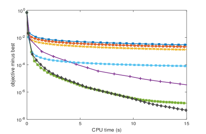
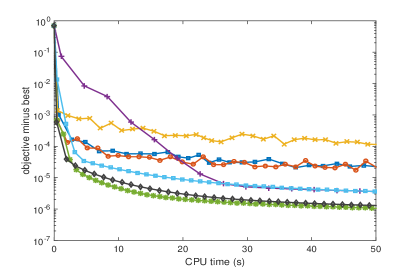
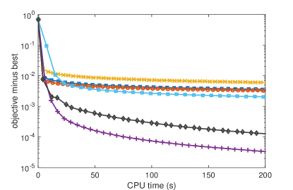
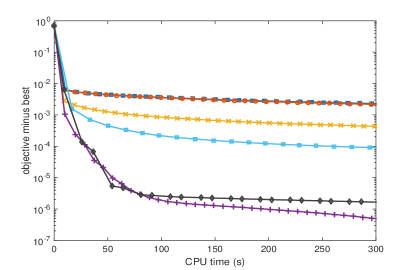
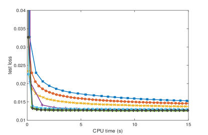
(a) protein

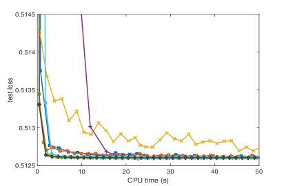
(b) covertype

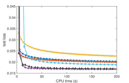
(c) mnist8m

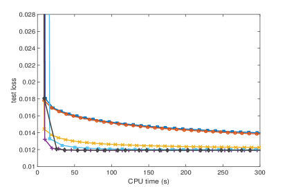
(d) dna

Figure 1: Performance vs CPU time (in sec) on graph-guided fused lasso (Top: objective value; Bottom: testing loss).

We perform experiments on the generalized lasso model $\sum_{i=1}^{n}\ell_{i}(x)+\|Ax\|_{1}$, where $\ell_{i}$ is the logistic loss on sample $i$, and $A$ is a matrix encoding the feature sparsity pattern. Here, we use graph-guided fused lasso [23] and set $A=[G;I]$, where $G$ is the sparsity pattern of the graph obtained by sparse inverse covariance estimation [32]. For the ADMM formulation, we introduce an additional variable $y$ and the constraint $Ax=y$. Experiments are performed on four benchmark data sets (Table II). We use a mini-batch size of $b=100$ on protein and covertype; and $b=500$ on mnist8m and dna. Experiments are performed on a PC with Intel i7-3770 $3.4$GHz CPU and $32$GB RAM,

TABLE II: Data sets for graph-guided fused lasso.

	#training	#test	dimensionality
protein	72,876	72,875	74
covertype	290,506	290,506	54
mnist8m	1,404,756	351,189	784
dna	2,400,000	600,000	800

All methods listed in Table I are compared and in Matlab. The proposed SVRG-ADMM uses the linearized update in (12) and $m=2n/b$. For further speedup, we simply use the last iterates in each stage ($x_{m},y_{m},u_{m}$) as $\tilde{x}_{s},\tilde{y}_{s},\tilde{u}_{s}$ in step 12 of Algorithms 1 and 2. Both SAG-ADMM and SVRG-ADMM are initialized by running OPG-ADMM for $n/b$ iterations. For SVRG-ADMM, since the learning rate in (12) is effectively $\eta/\gamma$, we set $\gamma=1$ and only tune $\eta$. All parameters are tuned as in [11]. Each stochastic algorithm is run on a small training subset for a few data passes (or stages). The parameter setting with the smallest training objective is then chosen. To ensure that the ADMM constraint is satisfied, we report the performance based on $(x_{t},Ax_{t})$. Results are averaged over five repetitions.

Figure 1 shows the objective values and testing losses versus CPU time. SAG-ADMM cannot be run on mnist8m and dna because of its large memory requirement (storing the weights already takes 8.2GB for mnist8m, and 14.3GB for dna). As can be seen, stochastic ADMM methods with variance reduction (SVRG-ADMM, SAG-ADMM and SDCA-ADMM) have fast convergence, while those that do not use variance reduction are much slower. SVRG-ADMM, SAG-ADMM and SDCA-ADMM have comparable speeds, but SVRG-ADMM requires much less storage (see also Table I). On the medium-sized protein and covertype, SCAS-ADMM has comparable performance with the other stochastic ADMM variants using variance reduction. However, it becomes much slower on the larger minist8m and dna, which is consistent with the analysis in Section III-D.

IV-B Multitask Learning

When there are a large number of outputs, the much smaller space requirement of SVRG-ADMM is clearly advantageous. In this section, experiments are performed on an $1000$-class ImageNet data set [33]. We use 1,281,167 images for training, and $50,000$ images for testing. $4096$ features are extracted from the last fully connected layer of the convolutional net VGG-16 [34]. The multitask learning problem is formulated as: $\min_{X}\sum_{i=1}^{N}\ell_{i}(X)+\lambda_{1}\|X\|_{1}+\lambda_{2}\|X\|_{*}$, where $X\in{\mathbb{R}}^{d\times N}$ is the parameter matrix, $N$ is the number of tasks, $d$ is the feature dimensionality, $\ell_{i}$ is the multinomial logistic loss on the $i$th task, and $\|\cdot\|_{*}$ is the nuclear norm. To solve this problem using ADMM, we introduce an additional variable $X^{\prime}$ with the constraint $X^{\prime}=X$. On setting $A=[I;I]$, the regularizer is then $g(AX)=g([X;X^{\prime}])=\lambda_{1}\|X\|_{1}+\lambda_{2}\|X^{\prime}\|_{*}$. We set $\lambda_{1}=10^{-5}$, $\lambda_{2}=10^{-4}$, and use a mini-batch size $b=500$. SAG-ADMM requires 38.2TB for storing the weights, and SDCA-ADMM 9.6GB for the dual variables, while SVRG-ADMM requires 62.5MB for storing $\tilde{x}$ and the full gradient.

Figure 2 shows the objective value and testing error versus time. SVRG-ADMM converges rapidly to a good solution. The other non-variance-reduced stochastic ADMM algorithms are very aggressive initially, but quickly get much slower. SCAS-ADMM is again slow on this large data set.

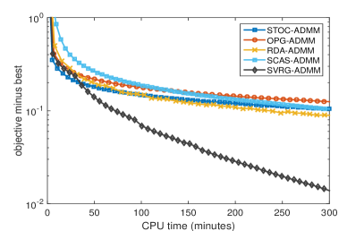
(a) objective.

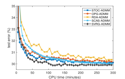
(b) testing error (%).

Figure 2: Performance vs CPU time (in min) on ImageNet.

IV-C Varying $\rho$

Finally, we perform experiments on total-variation (TV) regression [7] to demonstrate the effect of $\rho$. Samples $z_{i}$’s are generated with i.i.d. components from the standard normal distribution. Each $z_{i}$ is then normalized to $\|z_{i}\|=1$. The parameter $x$ is generated according to http://www.stanford.edu/~boyd/papers/admm/. The output $o_{i}$ is obtained by adding standard Gaussian noise to $x^{T}z_{i}$. Given $n$ samples $\{(z_{1},o_{1}),\dots,(z_{n},o_{n})\}$, TV regression is formulated as: $\min_{x}\frac{1}{2n}\sum_{i=1}^{n}\|o_{i}-x^{T}z_{i}\|^{2}+\lambda\|Ax\|_{1}$, where $A_{ij}=1$ if $i=j$; $-1$ if $j=i+1$; and 0 otherwise.

We set $n=100,000,d=500$, $\lambda=0.1/\sqrt{n}$, and a mini-batch size $b=100$. Figure 3 shows the objective value and testing loss versus CPU time, with different $\rho$’s. As can be seen, $\rho_{*}$ in Proposition 3 outperforms the other choices of $\rho$.

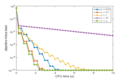
(a) objective.

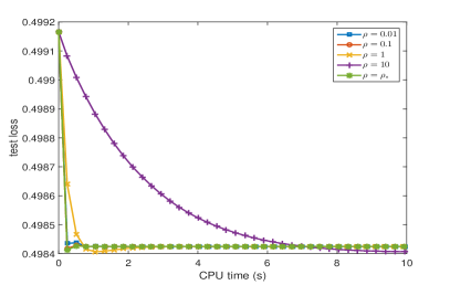
(b) testing loss.

Figure 3: Performance of SVRG-ADMM at different $\rho$’s.

IV-D Nonconvex Graph-Guided Fused Lasso

In this section, we compare the performance of the convex and nonconvex graph-guided fused lasso models. The nonconvex graph-guided fused lasso model is given by

$$\frac{1}{n}\sum_{i=1}^{n}\frac{1}{1+\exp(o_{i}z_{i}^{T}x)}+\lambda\|Ax\|_{1}.$$

For the convex model, we simply replace the sigmod loss with the logistic loss. The data sets used are summarized in Table III. Moreover, we use $\lambda=10^{-4}$ for a9a, news20, and $\lambda=10^{-5}$ for protein and covertype. The test errors are shown in Figure 4. As can be seen, the nonconvex model obtains better results on the data sets a9a, news20 and covertype, while maintaining good convergence speed.

TABLE III: Data sets for nonconvex graph-guided fused lasso.

	#training	#test	dimensionality
a9a	32,561	16,281	123
news20	12,995	3,247	100
protein	72,876	72,875	74
covertype	290,506	290,506	54

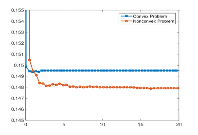
(a) a9a.

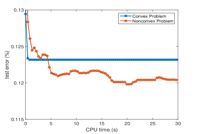
(b) news20.

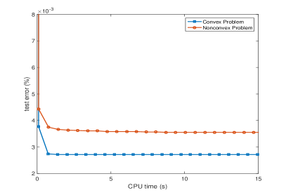
(c) protein.

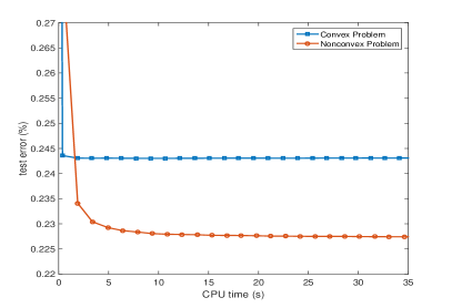
(d) covertype.

Figure 4: Test error $(\%)$ vs CPU time (in sec) for the convex and nonconvex models.

V Conclusion

This paper proposed a non-trivial integration of SVRG and ADMM. Its theoretical convergence rates for convex problems are as fast as existing variance-reduced stochastic ADMM algorithms, but its storage requirement is much lower, even independent of the sample size. Besides, we also show the convergence rate of the proposed method on nonconvex problems. Experimental results demonstrate its benefits over other stochastic ADMM methods and the benefits of using a nonconvex model.

References

- [1] L. Bottou, “Stochastic learning,” in Advanced Lectures on Machine Learning. Springer Verlag, 2004, pp. 146–168.
- [2] N. Parikh and S. Boyd, “Proximal algorithms,” Foundations and Trends in Optimization, vol. 1, no. 3, pp. 127–239, 2014.
- [3] A. Defazio, F. Bach, and S. Lacoste-Julien, “SAGA: A fast incremental gradient method with support for non-strongly convex composite objectives,” in Advances in Neural Information Processing Systems, 2014, pp. 2116–2124.
- [4] R. Johnson and T. Zhang, “Accelerating stochastic gradient descent using predictive variance reduction,” in Advances in Neural Information Processing Systems, 2013, pp. 315–323.
- [5] N. Roux, M. Schmidt, and F. Bach, “A stochastic gradient method with an exponential convergence rate for finite training sets,” in Advances in Neural Information Processing Systems, 2012, pp. 2663–2671.
- [6] S. Shalev-Shwartz and T. Zhang, “Stochastic dual coordinate ascent methods for regularized loss,” Journal of Machine Learning Research, vol. 14, no. 1, pp. 567–599, 2013.
- [7] S. Boyd, N. Parikh, E. Chu, B. Peleato, and J. Eckstein, “Distributed optimization and statistical learning via the alternating direction method of multipliers,” Foundations and Trends in Machine Learning, vol. 3, no. 1, pp. 1–122, 2011.
- [8] H. Ouyang, N. He, L. Tran, and A. Gray, “Stochastic alternating direction method of multipliers,” in Proceedings of the 30th International Conference on Machine Learning, 2013, pp. 80–88.
- [9] T. Suzuki, “Dual averaging and proximal gradient descent for online alternating direction multiplier method,” in Proceedings of the 30th International Conference on Machine Learning, 2013, pp. 392–400.
- [10] H. Wang and A. Banerjee, “Online alternating direction method,” in Proceedings of the 29th International Conference on Machine Learning, 2012, pp. 1119–1126.
- [11] W. Zhong and J. Kwok, “Fast stochastic alternating direction method of multipliers,” in Proceedings of the 31st International Conference on Machine Learning, 2014, pp. 46–54.
- [12] T. Suzuki, “Stochastic dual coordinate ascent with alternating direction method of multipliers,” in Proceedings of the 31st International Conference on Machine Learning, 2014, pp. 736–744.
- [13] S. Y. Zhao, W. J. Li, and Z. H. Zhou, “Scalable stochastic alternating direction method of multipliers,” Tech. Rep. arXiv:1502.03529, 2015.
- [14] Y. Shen, Z. Wen, and Y. Zhang, “Augmented lagrangian alternating direction method for matrix separation based on low-rank factorization,” Optimization Methods and Software, vol. 29, no. 2, pp. 239–263, 2014.
- [15] A. P. Liavas and N. D. Sidiropoulos, “Parallel algorithms for constrained tensor factorization via alternating direction method of multipliers,” IEEE Transactions on Signal Processing, vol. 63, no. 20, pp. 5450–5463, 2015.
- [16] B. Jiang, T. Lin, S. Ma, and S. Zhang, “Structured nonconvex and nonsmooth optimization: Algorithms and iteration complexity analysis,” arXiv preprint arXiv:1605.02408, 2016.
- [17] M. Hong, Z. Q. Luo, and M. Razaviyayn, “Convergence analysis of alternating direction method of multipliers for a family of nonconvex problems,” SIAM Journal on Optimization, vol. 26, no. 1, pp. 337–364, 2016.
- [18] G. Li and T. K. Pong, “Global convergence of splitting methods for nonconvex composite optimization,” SIAM Journal on Optimization, vol. 25, no. 4, pp. 2434–2460, 2015.
- [19] F. Wang, W. Cao, and Z. Xu, “Convergence of multi-block bregman admm for nonconvex composite problems,” arXiv preprint arXiv:1505.03063, 2015.
- [20] Y. Wang, W. Yin, and J. Zeng, “Global convergence of admm in nonconvex nonsmooth optimization,” arXiv preprint arXiv:1511.06324, 2015.
- [21] R. Nishihara, L. Lessard, B. Recht, A. Packard, and M. I. Jordan, “A general analysis of the convergence of ADMM,” in Proceedings of the 32nd International Conference on Machine Learning, 2015, pp. 343–352.
- [22] W. Deng and W. Yin, “On the global and linear convergence of the generalized alternating direction method of multipliers,” Journal of Scientific Computing, pp. 1–28, 2015.
- [23] S. Kim, K. A. Sohn, and E. P. Xing, “A multivariate regression approach to association analysis of a quantitative trait network,” Bioinformatics, vol. 25, no. 12, pp. i204–i212, 2009.
- [24] L. Jacob, G. Obozinski, and J.-P. Vert, “Group lasso with overlap and graph lasso,” in Proceedings of the 26th Annual International Conference on Machine Learning, 2009, pp. 433–440.
- [25] E. Ghadimi, A. Teixeira, I. Shames, and M. Johansson, “Optimal parameter selection for the alternating direction method of multipliers (ADMM): Quadratic problems,” IEEE Transactions on Automatic Control, vol. 60, no. 3, pp. 644–658, 2015.
- [26] P. Giselsson and S. Boyd, “Diagonal scaling in Douglas-Rachford splitting and ADMM,” in Proceedings of the 53rd IEEE Conference on Decision and Control, 2014.
- [27] X. Zhang, M. Burger, and S. Osher, “A unified primal-dual algorithm framework based on Bregman iteration,” Journal of Scientific Computing, vol. 46, no. 1, pp. 20–46, 2011.
- [28] G. Golub and C. Van Loan, Matrix Computations. JHU Press, 2012.
- [29] B. He and X. Yuan, “On the convergence rate of the Douglas-Rachford alternating direction method,” SIAM Journal on Numerical Analysis, vol. 50, no. 2, pp. 700–709, 2012.
- [30] L. Xiao and T. Zhang, “A proximal stochastic gradient method with progressive variance reduction,” SIAM Journal on Optimization, vol. 24, no. 4, 2014.
- [31] R. T. Rockafellar and R. J. Wets, Variational analysis. Springer Science & Business Media, 2009, vol. 317.
- [32] J. Friedman, T. Hastie, and R. Tibshirani, “Sparse inverse covariance estimation with the graphical lasso,” Biostatistics, vol. 9, no. 3, pp. 432–441, 2008.
- [33] O. Russakovsky, J. Deng, H. Su, J. Krause, S. Satheesh, S. Ma, Z. Huang, A. Karpathy, A. Khosla, M. Bernstein, A. C. Berg, and L. F.-F., “Imagenet large scale visual recognition challenge,” International Journal of Computer Vision, vol. 115, no. 3, pp. 211–252, 2015.
- [34] K. Simonyan and A. Zisserman, “Very deep convolutional networks for large-scale image recognition,” Tech. Rep. arXiv:1409.1556, 2014.