Finite sample breakdown point of Tukey’s halfspace median

Tukey’s halfspace median (HM), servicing as the multivariate counterpart of the univariate median, has been introduced and extensively studied in the literature. It is supposed and expected to preserve robustness property (the most outstanding property) of the univariate median. One of prevalent quantitative assessments of robustness is finite sample breakdown point (FSBP). Indeed, the FSBP of many multivariate medians have been identified, except for the most prevailing one—the Tukey’s halfspace median. This paper presents a precise result on FSBP for Tukey’s halfspace median. The result here depicts the complete prospect of the global robustness of HM in the finite sample practical scenario, revealing the dimension effect on the breakdown point robustness and complimenting the existing asymptotic breakdown point result.

Key words: Tukey depth; Tukey median; Breakdown point; In general position

2000 Mathematics Subject Classification Codes: 62F10; 62F40; 62F35

1 Introduction

Robustness (as an insurance) is one of the most desirable properties for any statistical procedures. The most outstanding feature of univariate median is its robustness. Indeed, among all translation equivariant location estimators, it has the best possible breakdown point (Donoho, 1982) (and minimum maximum bias if underlying distribution has unimodal symmetric density (Huber, 1964)).

It is very much desirable to extend the univariate median to multidimensional settings and meanwhile inherit/preserve its outstanding robustness for multidimensional data. In fact, the earliest attempt of this type of extension was made at least one century ago (Weber, 1909). Oja’s median (Oja, 1983) is another promising extension.

On the other hand, defining the multi-dimensional median as the deepest point of the underlying multidimensional data is an obvious natural approach. Serving this purpose, general notions of data depth have been proposed and studied (Zuo and Serfling, 2000). The main goal of data depth is to provide a center-outward ordering of multidimensional observations. Multivariate medians as the deepest point (the generalization of the univariate median) therefore have been naturally introduced and examined. Among the depth induced multidimensional medians, Tukey’s halfspace median (Tukey, 1975) is the most prominent and prevailing. Robustness is of course the main targeted property to be shared by all depth induced medians.

There are many ways to measure the robustness of a statistical procedure (especially location estimators). Among others, maximum bias, influence function and finite sample breakdown point (FSBP) are the most standard gauges. FSBP by far is the most prevailing quantitative assessment of robustness due to its plain definition (without involvement of probability/randomness concept).

The concept of breakdown point was introduced by Hodges (1967) and Hampel (Ph. D. dissertation (1968), Univ. California, Berkeley) and extended by Hampel (1971) and developed further by, among others, Huber (1981). It has proved most successful in the context of location, scale and regression problems. Finite sample version of breakdown point has been proposed, promoted and popularized by Donoho (1982) and Donoho and Huber (1983) (DH83).

The seminar paper of Donoho and Gasko (1992) (hereafter DG92) was devoted to extensively study the FSBP of multivariate location estimators including Tukey’s halfspace depth induced location estimators, especially the halfspace median (HM). Specifically, DG92 established FSBP for many location estimators, including the lower bound of FSBP for halfspace median. However, lower bound contains much scarce information about FSBP of HM. What is the exact FSBP of HM is still an open question.

Adrover and Yohai (2002) and Chen and Tyler (2002) have pioneered in studying the maximum bias of HM. It is found that the asymptotic breakdown point of HM is $1/3$, as also given in DG92 (see also Chen (1995) and Mizera (2002)). The latter result however is obtained restricted to a sub-class of distributions (the absolutely continuous centrosymemetric ones) in the maximum bias definition, and when sample size $n$ approaches to the infinity. Ironically, DG92 only provided the asymptotic breakdown point for HM and uncharacteristically left its FSBP open. Furthermore, the former does not provide any clue of the dimensional effect on the breakdown robustness and its behavior in finite sample practical scenario. To address this issue and provide a definite answer is the main objective of this manuscript.

Let’s end this section with some definitions. A location statistical functional $T$ in $\mathcal{R}^{d}$ ($d\geq 1$) is said to be affine equivariant if

$$T(\Sigma\mathcal{X}^{n}+\textbf{\emph{b}})=\Sigma T(\mathcal{X}^{n})+\textbf{\emph{b}},$$

for any $d\times d$ nonsingular matrix $\Sigma$ and $\textbf{\emph{b}}\in R^{d}$, where $\Sigma\mathcal{X}^{n}+\textbf{\emph{b}}=\{\Sigma X_{1}+\textbf{\emph{b}},\cdots,\Sigma X_{n}+\textbf{\emph{b}}\}$ and $X_{1},\cdots,X_{n}$ is a given random sample in $\mathcal{R}^{d}$ (denote $\mathcal{X}^{n}=\{X_{1},\cdots,X_{n}\}$ hereafter). When $d=1$ and $\Sigma=1$, we call $T$ is translation equivariant.

Define the depth of a point x with respect to $\mathcal{X}^{n}\subset\mathcal{R}^{d}$ as

$$D(\textbf{\emph{x}},\mathcal{X}^{n})=\inf_{\textbf{\emph{u}}\in\mathcal{S}^{d-1}}P_{n}(\textbf{\emph{u}}^{\top}X\leq\textbf{\emph{u}}^{\top}\textbf{\emph{x}}),$$

where $\mathcal{S}^{d-1}=\{\textbf{\emph{z}}\in\mathcal{R}^{d}:\|\textbf{\emph{z}}\|=1\}$, and $P_{n}$ denotes the empirical probability measure and $\|\cdot\|$ stands for Euclidean norm. Denote

$$\mathcal{M}(\mathcal{X}^{n})=\{\textbf{\emph{x}}:D(\textbf{\emph{x}},\mathcal{X}^{n})=\lambda^{*}(\mathcal{X}^{n})\},$$

where $\lambda^{*}(\mathcal{X}^{n})=\sup_{\textbf{\emph{x}}}D(\textbf{\emph{x}},\mathcal{X}^{n})$. Tukey’s halfspace median is defined as,

$$T^{*}(\mathcal{X}^{n})=\textbf{Ave}\left\{\textbf{\emph{x}}\in\mathcal{M}(\mathcal{X}^{n})\right\},$$

i.e., the average of all points that maximize $D(\textbf{\emph{x}},\mathcal{X}^{n})$. Clearly, when $d=1$, $T^{*}(\mathcal{X}^{n})$ reduces to the univariate sample median.

The finite sample additional breakdown point (ABP) of a location estimator $T$ at the given sample $\mathcal{X}^{n}$ is defined as

$$ABP(T,\mathcal{X}^{n})=\min_{1\leq m\leq n}\left\{\frac{m}{n+m}:\sup_{\mathcal{Y}^{m}}\left\|T(\mathcal{X}^{n}\cup\mathcal{Y}^{m})-T(\mathcal{X}^{n})\right\|=\infty\right\},$$

where $\mathcal{Y}^{m}$ denotes an arbitrary contaminating sample of size $m$, adjoining to $\mathcal{X}^{n}\subset\mathcal{R}^{d}$. Namely, the ABP of an estimator is the minimum additional fraction which could drive the estimator beyond any bound. It is readily seen that the ABP of the sample mean and the univariate median are $1/(n+1)$ and $1/2$, respectively. The latter is the best that one can expect for any translation equivariant location estimator (Donoho, 1982).

Additional breakdown point is one of the forms of the finite sample breakdown point notion, replacement breakdown point (RBP) is the other one (DH83), where instead of adding contaminating points to $\mathcal{X}^{n}$, replacing $m$ points of $\mathcal{X}^{n}$ by $m$ arbitrary points. Some prefer RBP since it is arguably more close to the contamination in reality. The two are actually equivalent in the sense of Zuo (2001). Further discussions on FSBP concept could be found in DH83 and Lopuhaä and Rousseeuw (1991). By FSBP we mean ABP in the sequel.

We anticipate that the approach and results here may be extended for the investigating the FSBP of estimators that are related to Tukey’s halfspace depth function such as multiple-output quantile regression estimators (Hallin et al., 2010), the maximum regression depth estimator (Rousseeuw and Hubert, 1999), and probably the functional halfspace depth estimators (López-Pintado and Romo, 2009).

The remainder of this article is organized as follows. Section 2 presents three preliminary lemmas for the main results, which will be proved in Section 3. The article ends in Section 4 with some concluding remarks.

2 Three preliminary lemmas

Since the proof of the main result is rather complicated and long, we divide it into several parts and present some of them as lemmas. In this section, three preliminary lemmas are established. They play important roles in the proof of the main results.

Without loss of generality, we assume that $\mathcal{X}^{n}$ is in general position (IGP hereafter) throughout this paper. That is, no more than $d$ sample points lie in a $(d-1)$-dimensional hyperplane. This assumption is common in the literature involving statistical depth functions and breakdown point robustness (Donoho and Gasko, 1992; Mosler et al., 2009). Since HM reduces to the sample median and its FSBP is known as $1/2$ for $d=1$, we only focus on $d\geq 2$ in the sequel.

For $\mathcal{X}^{n}$, under the IGP assumption, there must exist $N_{n}^{d}={n\choose d}$ unit vectors, say $\mu_{j}\in\mathcal{S}^{d-1}$, $j=1,2,\cdots,N_{n}^{d}$, such that they are respectively normal to $N_{n}^{d}$ hyperplanes with each of which passing through $d$ observations. Since $N_{n}^{d}$ is finite when $n$ and $d$ are fixed, we can find a unit vector, say u, satisfying

$$\textbf{\emph{u}}^{\top}\mu_{j}\neq 0,\quad\text{ for }\forall j\in\left\{1,2,\cdots,N_{n}^{d}\right\}.$$ (1)

For simplicity, for any given $\textbf{\emph{u}}\in\mathcal{S}^{d-1}$, in the sequel we denote

$$\mathbb{A}_{\textbf{\emph{u}}}=(\textbf{\emph{u}}_{1},\textbf{\emph{u}}_{2},\cdots,\textbf{\emph{u}}_{d-1}),$$ (2)

where $\textbf{\emph{u}}_{1},\textbf{\emph{u}}_{2},\cdots,\textbf{\emph{u}}_{d-1}$ are orthogonal to u, and together with u, they form a set of standard basis vectors of $\mathcal{R}^{d}$. Remarkably, although the choice of $\textbf{\emph{u}}_{1},\textbf{\emph{u}}_{2},\cdots,\textbf{\emph{u}}_{d-1}$ is not unique when $d\geq 2$, this fact does not effect the proofs presented in the rest of this paper due to the affine equivariance of HM and its related Tukey depth, nevertheless. Hence, we pretend that $\mathbb{A}_{\textbf{\emph{u}}}$ is unique in the sequel.

Write $\mathbf{x}_{i}=\mathbb{A}_{\textbf{\emph{u}}}^{\top}X_{i}$, $i=1,2,\cdots,n$, and $\mathbf{X}_{\textbf{\emph{u}}}^{n}=\{\mathbf{x}_{1},\mathbf{x}_{2},\cdots,\mathbf{x}_{n}\}$, call it $\mathbb{A}_{\textbf{\emph{u}}}$-projections of $\mathcal{X}^{n}$ hereafter. It will greatly facilitate our discussion, if $\mathbf{X}_{\textbf{\emph{u}}}^{n}$ is still in general position. Fortunately, Lemma 1 provides a positive answer.

Lemma 1. Suppose $\mathcal{X}^{n}$ is IGP, and $\textbf{\emph{u}}\in\mathcal{S}^{d-1}$ satisfies display (1). Then $\mathbf{X}_{\textbf{\emph{u}}}^{n}=\{\mathbf{x}_{1},\mathbf{x}_{2}$, $\cdots,\mathbf{x}_{n}\}\subset\mathcal{R}^{d-1}$ is in general position too when $d\geq 2$.

Proof. If $\mathbf{X}_{\textbf{\emph{u}}}^{n}$ is not IGP, then there must exist a $(d-2)$-dimensional hyperplane $\mathcal{P}_{1}$ containing at least $d$ $\mathbb{A}_{\textbf{\emph{u}}}$-projections, say $\mathbf{x}_{i_{1}},\mathbf{x}_{i_{2}},\cdots,\mathbf{x}_{i_{k}}$ ($k\geq d$). Let $\mathbf{v}\in\mathcal{S}^{d-2}$ be the normal vector of $\mathcal{P}_{1}$. Then, we have

$$\mathbf{v}^{\top}\mathbf{x}_{i_{1}}=\mathbf{v}^{\top}\mathbf{x}_{i_{2}}=\cdots=\mathbf{v}^{\top}\mathbf{x}_{i_{k}}.$$

Recalling the definition of $\mathbf{x}_{i}$, we further obtain

$$(\mathbb{A}_{\textbf{\emph{u}}}\mathbf{v})^{\top}X_{i_{1}}=(\mathbb{A}_{\textbf{\emph{u}}}\mathbf{v})^{\top}X_{i_{2}}=\cdots=(\mathbb{A}_{\textbf{\emph{u}}}\mathbf{v})^{\top}X_{i_{k}}.$$ (3)

Write $\widetilde{\textbf{\emph{v}}}=\mathbb{A}_{\textbf{\emph{u}}}\mathbf{v}$. Clearly, $\widetilde{\textbf{\emph{v}}}\in\mathcal{R}^{d}$ and $(\widetilde{\textbf{\emph{v}}})^{\top}\widetilde{\textbf{\emph{v}}}=1$, namely, $\widetilde{\textbf{\emph{v}}}\in\mathcal{S}^{d-1}$. Hence, (3) implies that one can find a $(d-1)$-dimensional hyperplane, with $\widetilde{\textbf{\emph{v}}}$ being its normal vector, that passes through $k$ observations. This contradicts with the IGP assumption of $\mathcal{X}^{n}$ if $k>d$. When $k=d$, (3) implies $\widetilde{\textbf{\emph{v}}}\in\{\mu_{j}\}_{j=1}^{N_{n}^{d}}$. This obviously contradicts with the fact that u satisfies (1) due to $\widetilde{\textbf{\emph{v}}}^{\top}\textbf{\emph{u}}=\mathbf{v}^{\top}\mathbb{A}_{\textbf{\emph{u}}}^{\top}\textbf{\emph{u}}=0$. This completes the proof of this lemma. $\Box$

Remark 2.1 In fact, $\mathcal{X}^{n}$ is IGP if and only if $\mathbf{X}_{\textbf{\emph{u}}}^{n}$ is IGP for u satisfying (1).

To derive the FSBP of HM, we need to investigate the maximum Tukey depth with respect to the $\mathbb{A}_{\textbf{\emph{u}}}$-projections of $\mathcal{X}^{n}$. The following Lemma 2 will play an important role during this process.

We formally introduce some additional necessary notations as follows. For $\forall\textbf{\emph{x}},\textbf{\emph{y}}\in\mathcal{R}^{d}$, let

$$\mathcal{U}_{\textbf{\emph{x}}} = \{\textbf{\emph{u}}\in\mathcal{S}^{d-1}:~{}P_{n}(\textbf{\emph{u}}^{\top}X\leq\textbf{\emph{u}}^{\top}\textbf{\emph{x}})=D(\textbf{\emph{x}},\mathcal{X}^{n})\}$$

be the set of all optimal vectors of x which realize the depth at x with respect to $\mathcal{X}^{n}$, and

$$\mathcal{H}_{\textbf{\emph{x}},\textbf{\emph{y}}} = \{\textbf{\emph{u}}\in\mathcal{S}^{d-1}:~{}\textbf{\emph{u}}^{\top}\textbf{\emph{x}}<\textbf{\emph{u}}^{\top}\textbf{\emph{y}}\}$$

the hemisphere determined by $\{\textbf{\emph{x}},\textbf{\emph{y}}\}$. Furthermore, for $\forall\textbf{\emph{z}}\in\mathcal{M}(\mathcal{X}^{n})$, let

$$\mathcal{A}_{\textbf{\emph{z}}} = \{\textbf{\emph{x}}\in\mathcal{M}(\mathcal{X}^{n}):\mathcal{U}_{\textbf{\emph{x}}}\cap\mathcal{H}_{\textbf{\emph{x}},\textbf{\emph{z}}}\neq\emptyset\},$$

$$\mathcal{B}_{\textbf{\emph{z}}} = \{\textbf{\emph{x}}\in\mathcal{M}(\mathcal{X}^{n}):\mathcal{U}_{\textbf{\emph{x}}}\cap\mathcal{H}_{\textbf{\emph{x}},\textbf{\emph{z}}}=\emptyset\},$$

$$\widetilde{\mathcal{B}}_{\textbf{\emph{z}}} = \mathcal{B}_{\textbf{\emph{z}}}\setminus\{\textbf{\emph{z}}\}.$$

Obviously, (i) $\mathcal{M}(\mathcal{X}^{n})=\mathcal{A}_{\textbf{\emph{z}}}\cup\mathcal{B}_{\textbf{\emph{z}}}$, (ii) $\mathcal{A}_{\textbf{\emph{z}}}\cap\mathcal{B}_{\textbf{\emph{z}}}=\emptyset$, (iii) $\textbf{\emph{z}}\in\mathcal{B}_{\textbf{\emph{z}}}$ because $\mathcal{H}_{\textbf{\emph{z}},\textbf{\emph{z}}}=\emptyset$.

For $\mathcal{U}_{\textbf{\emph{x}}}$, $\mathcal{B}_{\textbf{\emph{x}}}$ and $\widetilde{\mathcal{B}}_{\textbf{\emph{z}}}$, Lemma 2 below depicts several important properties of them.

Lemma 2. Suppose $\mathcal{X}^{n}$ is IGP and $\mathcal{M}(\mathcal{X}^{n})$ is of affine dimension $d$. For $\forall\textbf{\emph{z}}_{1}$ lying in the interior of $\mathcal{M}(\mathcal{X}^{n})$, if $\widetilde{\mathcal{B}}_{\textbf{\emph{z}}_{1}}\neq\emptyset$, then:

1. (o1) for $\forall\textbf{\emph{u}}\in\mathcal{U}_{\textbf{\emph{z}}_{1}}$ and $\forall\textbf{\emph{z}}\in\widetilde{\mathcal{B}}_{\textbf{\emph{z}}_{1}}$, we have $\textbf{\emph{u}}^{\top}\textbf{\emph{z}}\geq\textbf{\emph{u}}^{\top}\textbf{\emph{z}}_{1}$.

2. (o2) for $\forall\textbf{\emph{z}}\in\mathcal{B}_{\textbf{\emph{z}}_{1}}$, we have $\mathcal{U}_{\textbf{\emph{z}}}\subset\mathcal{U}_{\textbf{\emph{z}}_{1}}$.

3. (o3) for $\forall\textbf{\emph{z}}\in\widetilde{\mathcal{B}}_{\textbf{\emph{z}}_{1}}$, we have $\mathcal{B}_{\textbf{\emph{z}}}\subset\mathcal{B}_{\textbf{\emph{z}}_{1}}$, but $\textbf{\emph{z}}_{1}\notin\mathcal{B}_{\textbf{\emph{z}}}$. That is, $\mathcal{B}_{\textbf{\emph{z}}}\subset\widetilde{\mathcal{B}}_{\textbf{\emph{z}}_{1}}$.

Proof. (o1). If not, $\textbf{\emph{u}}^{\top}\textbf{\emph{z}}<\textbf{\emph{u}}^{\top}\textbf{\emph{z}}_{1}$. Then $\lambda^{*}(\mathcal{X}^{n})\leq P_{n}(\textbf{\emph{u}}^{\top}X\leq\textbf{\emph{u}}^{\top}\textbf{\emph{z}})\leq P_{n}(\textbf{\emph{u}}^{\top}X\leq\textbf{\emph{u}}^{\top}\textbf{\emph{z}}_{1})=\lambda^{*}(\mathcal{X}^{n})$, resulting in $\textbf{\emph{u}}\in\mathcal{U}_{\textbf{\emph{z}}}\cap\mathcal{H}_{\textbf{\emph{z}},\textbf{\emph{z}}_{1}}$, and hence contradicting with $\textbf{\emph{z}}\in\mathcal{B}_{\textbf{\emph{z}}_{1}}$.

(o2). By definition, $\textbf{\emph{z}}\in\mathcal{B}_{\textbf{\emph{z}}_{1}}$ implies $\mathcal{U}_{\textbf{\emph{z}}}\cap\mathcal{H}_{\textbf{\emph{z}},\textbf{\emph{z}}_{1}}=\emptyset$. Hence, for $\forall\textbf{\emph{u}}\in\mathcal{U}_{\textbf{\emph{z}}}$, we have $\textbf{\emph{u}}^{\top}\textbf{\emph{z}}\geq\textbf{\emph{u}}^{\top}\textbf{\emph{z}}_{1}$. Then $\lambda^{*}(\mathcal{X}^{n})\leq P_{n}(\textbf{\emph{u}}^{\top}X\leq\textbf{\emph{u}}^{\top}\textbf{\emph{z}}_{1})\leq P_{n}(\textbf{\emph{u}}^{\top}X\leq\textbf{\emph{u}}^{\top}\textbf{\emph{z}})=\lambda^{*}(\mathcal{X}^{n})$. That is, $\textbf{\emph{u}}\in\mathcal{U}_{\textbf{\emph{z}}_{1}}$, and hence $\mathcal{U}_{\textbf{\emph{z}}}\subset\mathcal{U}_{\textbf{\emph{z}}_{1}}$.

(o3). For $\forall\textbf{\emph{x}}\in\mathcal{B}_{\textbf{\emph{z}}}$, $\mathcal{U}_{\textbf{\emph{x}}}\bigcap\mathcal{H}_{\textbf{\emph{x}},\textbf{\emph{z}}}=\emptyset$. Hence, $\textbf{\emph{u}}_{\textbf{\emph{x}}}^{\top}(\textbf{\emph{x}}-\textbf{\emph{z}})\geq 0$ for $\forall\textbf{\emph{u}}_{\textbf{\emph{x}}}\in\mathcal{U}_{\textbf{\emph{x}}}$. Next, by (o2), we have $\mathcal{U}_{\textbf{\emph{x}}}\subset\mathcal{U}_{\textbf{\emph{z}}}\subset\mathcal{U}_{\textbf{\emph{z}}_{1}}$, which implies $\textbf{\emph{u}}_{\textbf{\emph{x}}}^{\top}\textbf{\emph{x}}\geq\textbf{\emph{u}}_{\textbf{\emph{x}}}^{\top}\textbf{\emph{z}}\geq\textbf{\emph{u}}_{\textbf{\emph{x}}}^{\top}\textbf{\emph{z}}_{1}$ by (o1). That is, $\mathcal{U}_{\textbf{\emph{x}}}\bigcap\mathcal{H}_{\textbf{\emph{x}},\textbf{\emph{z}}_{1}}=\emptyset$, which implies $\textbf{\emph{x}}\in\mathcal{B}_{\textbf{\emph{z}}_{1}}$, and hence $\mathcal{B}_{\textbf{\emph{z}}}\subset\mathcal{B}_{\textbf{\emph{z}}_{1}}$.

Next, since $\textbf{\emph{z}}_{1}$ lies in the interior of $\mathcal{M}(\mathcal{X}^{n})$, we can find a small enough $\varepsilon>0$ such that $\{\textbf{\emph{x}}:\|\textbf{\emph{x}}-\textbf{\emph{z}}_{1}\|<\varepsilon\}\subset\mathcal{M}(\mathcal{X}^{n})$. For $\forall\textbf{\emph{u}}_{\textbf{\emph{z}}_{1}}\in\mathcal{U}_{\textbf{\emph{z}}_{1}}$, if the hyperplane $\{\textbf{\emph{x}}:\textbf{\emph{u}}_{\textbf{\emph{z}}_{1}}^{\top}(\textbf{\emph{x}}-\textbf{\emph{z}}_{1})=0\}$ contains a sample point, say $X_{1}$, then let $\widetilde{\textbf{\emph{z}}}_{1}=-\frac{1}{2}\varepsilon\textbf{\emph{u}}_{\textbf{\emph{z}}_{1}}+\textbf{\emph{z}}_{1}$. Clearly, $\widetilde{\textbf{\emph{z}}}_{1}\in\mathcal{M}(\mathcal{X}^{n})$, and $\textbf{\emph{u}}_{\textbf{\emph{z}}_{1}}^{\top}\widetilde{\textbf{\emph{z}}}_{1}<\textbf{\emph{u}}_{\textbf{\emph{z}}_{1}}^{\top}\textbf{\emph{z}}_{1}=\textbf{\emph{u}}_{\textbf{\emph{z}}_{1}}^{\top}X_{1}$. As a result, $D(\widetilde{\textbf{\emph{z}}}_{1},\mathcal{X}^{n})\leq P_{n}(\textbf{\emph{u}}_{\textbf{\emph{z}}_{1}}^{\top}X\leq\textbf{\emph{u}}_{\textbf{\emph{z}}_{1}}^{\top}\widetilde{\textbf{\emph{z}}}_{1})=P_{n}(\textbf{\emph{u}}_{\textbf{\emph{z}}_{1}}^{\top}X\leq\textbf{\emph{u}}_{\textbf{\emph{z}}_{1}}^{\top}\textbf{\emph{z}}_{1})-1/n=\lambda^{*}(\mathcal{X}^{n})-1/n$, contradicting with $\widetilde{\textbf{\emph{z}}}_{1}\in\mathcal{M}(\mathcal{X}^{n})$.

Hence, $\forall\textbf{\emph{u}}_{\textbf{\emph{z}}_{1}}\in\mathcal{U}_{\textbf{\emph{z}}_{1}}$, $\{\textbf{\emph{x}}:\textbf{\emph{u}}_{\textbf{\emph{z}}_{1}}^{\top}(\textbf{\emph{x}}-\textbf{\emph{z}}_{1})=0\}$ contains no sample point. This fact implies that there exists a permutation $(i_{1},i_{2},\cdots,i_{n})$ of $(1,2,\cdots,n)$ satisfying

$$\textbf{\emph{u}}_{\textbf{\emph{z}}_{1}}^{\top}X_{i_{1}}\leq\textbf{\emph{u}}_{\textbf{\emph{z}}_{1}}^{\top}X_{i_{2}}\leq\cdots\leq\textbf{\emph{u}}_{\textbf{\emph{z}}_{1}}^{\top}X_{i_{k^{*}}}<\textbf{\emph{u}}_{\textbf{\emph{z}}_{1}}^{\top}\textbf{\emph{z}}_{1}<$$

$$\textbf{\emph{u}}_{\textbf{\emph{z}}_{1}}^{\top}X_{i_{k^{*}+1}}\leq\cdots\leq\textbf{\emph{u}}_{\textbf{\emph{z}}_{1}}^{\top}X_{i_{n}},$$ (4)

where $k^{*}=n\lambda^{*}(\mathcal{X}^{n})$. Then similar to Liu et al. (2013), we have that a direction vector u should belong to $\mathcal{U}_{\textbf{\emph{z}}_{1}}$ if it satisfies

$$\left\{\begin{array}[]{ccc}\textbf{\emph{u}}^{\top}(X_{i_{1}}-\textbf{\emph{z}}_{1})&<&0\\ \textbf{\emph{u}}^{\top}(X_{i_{2}}-\textbf{\emph{z}}_{1})&<&0\\ \vdots&&\\ \textbf{\emph{u}}^{\top}(X_{i_{k^{*}}}-\textbf{\emph{z}}_{1})&<&0\\ \textbf{\emph{u}}^{\top}(\textbf{\emph{z}}_{1}-X_{i_{k^{*}+1}})&<&0\\ \vdots&&\\ \textbf{\emph{u}}^{\top}(\textbf{\emph{z}}_{1}-X_{i_{n}})&<&0.\end{array}\right.$$

Using this, it is trivial to check that $\mathcal{U}_{\textbf{\emph{z}}_{1}}$ is non-coplanar when $\textbf{\emph{z}}_{1}$ lies in the interior of $\mathcal{M}(\mathcal{X}^{n})$. Hence, there must exist $\textbf{\emph{v}}_{11},\textbf{\emph{v}}_{12},\cdots,\textbf{\emph{v}}_{1d}\in\mathcal{U}_{\textbf{\emph{z}}_{1}}$, which are of affine dimension $d$.

Observe that, $\forall\textbf{\emph{z}}\in\widetilde{\mathcal{B}}_{\textbf{\emph{z}}_{1}}$, there $\exists\widetilde{\textbf{\emph{v}}}\in\{\textbf{\emph{v}}_{11},\textbf{\emph{v}}_{12},\cdots,\textbf{\emph{v}}_{1d}\}$ satisfying

$$\widetilde{\textbf{\emph{v}}}^{\top}(\textbf{\emph{z}}-\textbf{\emph{z}}_{1})>0.$$ (6)

(If not, $\textbf{\emph{v}}_{1l}^{\top}(\textbf{\emph{z}}-\textbf{\emph{z}}_{1})=0$ for $l=1,2,\cdots,d$, which lead to $\textbf{\emph{z}}=\textbf{\emph{z}}_{1}$. This is impossible due to $\textbf{\emph{z}}\in\widetilde{\mathcal{B}}_{\textbf{\emph{z}}_{1}}$.) Hence, $\mathcal{U}_{\textbf{\emph{z}}_{1}}\cap\mathcal{H}_{\textbf{\emph{z}}_{1},z}\neq\emptyset$, and then $\textbf{\emph{z}}_{1}\notin\mathcal{B}_{\textbf{\emph{z}}}$. This completes the proof of (o3). $\Box$

Relying on Lemma 2, we are able to find a point $\textbf{\emph{x}}_{0}$ in the interior of $\mathcal{M}(\mathcal{X}^{n})$, which lies outside of at least one optimal halfspace of any $\textbf{\emph{x}}\neq\textbf{\emph{x}}_{0}$. Here by optimal halfspace of $x$ we mean the halfspace realizing the depth at $x$. That is, we have the following lemma.

Lemma 3. When $\mathcal{X}^{n}$ is IGP, there must exist an $\textbf{\emph{x}}_{0}\in\mathcal{M}(\mathcal{X}^{n})$ such that $\mathcal{U}_{\textbf{\emph{x}}}\bigcap\mathcal{H}_{\textbf{\emph{x}},\textbf{\emph{x}}_{0}}\neq\emptyset$ for $\forall\textbf{\emph{x}}\in\mathcal{R}^{d}\setminus\{\textbf{\emph{x}}_{0}\}$, i.e., we can find a $\textbf{\emph{u}}\in\mathcal{U}_{\textbf{\emph{x}}}$ satisfying $\textbf{\emph{u}}^{\top}\textbf{\emph{x}}<\textbf{\emph{u}}^{\top}\textbf{\emph{x}}_{0}$.

In the sequel the major task is to prove: $\mathcal{U}_{\textbf{\emph{x}}}\bigcap\mathcal{H}_{\textbf{\emph{x}},\textbf{\emph{x}}_{0}}\neq\emptyset$ for $\forall\textbf{\emph{x}}\in\mathcal{M}(\mathcal{X}^{n})\setminus\{\textbf{\emph{x}}_{0}\}$ when $d\geq 2$. It consists of three parts, i.e., (A), (B) and (C), related respectively to three scenarios of the affine dimension $\textbf{dim}(\mathcal{M})$ of $\mathcal{M}(\mathcal{X}^{n})$. Both (A) and (B) indicates that taking $\textbf{\emph{x}}_{0}=T^{*}(\mathcal{X}^{n})$ is valid, while (C) is technically much more difficult and the resulted $\textbf{\emph{x}}_{0}$ may $\neq T^{*}(\mathcal{X}^{n})$. In (C), we first obtain a candidate point, say $\bar{\textbf{\emph{z}}}_{0}$, through an iterative procedure consisting of three steps, i.e., (a), (b) and (c), and then show that $\bar{\textbf{\emph{z}}}_{0}$ can serve as $\textbf{\emph{x}}_{0}$. For convenience, we use the same notations (e.g., $\mathcal{X}^{n}$) as before in Lemma 2 though. Its result can be applied to any other IGP data set, nevertheless.

Proof. When $d=1$, by letting $\textbf{\emph{x}}_{0}$ be the sample median, the proof is trivial. When $d\geq 2$, for $\forall\textbf{\emph{x}}\notin\mathcal{M}(\mathcal{X}^{n})$ and $\forall\textbf{\emph{z}}\in\mathcal{M}(\mathcal{X}^{n})$, we claim $\mathcal{U}_{\textbf{\emph{x}}}\cap\mathcal{H}_{\textbf{\emph{x}},\textbf{\emph{z}}}\neq\emptyset$. If not, for $\forall\textbf{\emph{u}}\in\mathcal{U}_{\textbf{\emph{x}}}$, we have $\textbf{\emph{u}}^{\top}\textbf{\emph{x}}\geq\textbf{\emph{u}}^{\top}\textbf{\emph{z}}$, which leads to $\lambda^{*}(\mathcal{X}^{n})\leq P_{n}(\textbf{\emph{u}}^{\top}X\leq\textbf{\emph{u}}^{\top}\textbf{\emph{z}})\leq P_{n}(\textbf{\emph{u}}^{\top}X\leq\textbf{\emph{u}}^{\top}\textbf{\emph{x}})=D(\textbf{\emph{x}},\mathcal{X}^{n})$, contradicting the definition of $\lambda^{*}$ and $\mathcal{M}(\mathcal{X}^{n})$. In the sequel we show that there $\exists\textbf{\emph{x}}_{0}\in\mathcal{M}(\mathcal{X}^{n})$ satisfying $\mathcal{U}_{\textbf{\emph{x}}}\bigcap\mathcal{H}_{\textbf{\emph{x}},\textbf{\emph{x}}_{0}}\neq\emptyset$ for $\forall\textbf{\emph{x}}\in\mathcal{M}(\mathcal{X}^{n})\setminus\{\textbf{\emph{x}}_{0}\}$.

(A) Scenario $\textbf{dim}(\mathcal{M})=0$. Since $\mathcal{M}(\mathcal{X}^{n})=\{T^{*}(\mathcal{X}^{n})\}$, Lemma 3 already holds by letting $\textbf{\emph{x}}_{0}=T^{*}(\mathcal{X}^{n})$.

(B) Scenario $0<\textbf{dim}(\mathcal{M})<d$. We now show that taking $\textbf{\emph{x}}_{0}=T^{*}(\mathcal{X}^{n})$ is valid.

Relying on Theorem 4.2 of Paindaveine and Šiman (2011), it is easy to check that there $\exists\mu_{*}\in\{\mu_{j}\}_{j=1}^{N_{n}^{d}}$ normal to the hyperplane $\Pi_{0}=\{\textbf{\emph{z}}\in\mathcal{R}^{d}:\mu_{*}^{\top}\textbf{\emph{z}}=q_{*}\}$ such that: (i) $\Pi_{0}\supset\mathcal{M}(\mathcal{X}^{n})$, (ii) $\Pi_{0}$ contains $d$ observations, say $\mathbf{Z}_{d}:=\{X_{k_{1}},X_{k_{2}},\cdots,X_{k_{d}}\}$. Here $q_{*}=\inf\{t\in\mathcal{R}^{1}:P_{n}(\mu_{*}^{\top}X\leq t)\geq\lambda^{*}(\mathcal{X}^{n})\}$.

Obviously, $\mathcal{M}(\mathcal{X}^{n})\subset\textbf{cov}(\mathbf{Z}_{d})$, i.e., the convex hull of $\mathbf{Z}_{d}$. If not, one may deviate $\Pi_{0}$ around a point $\textbf{\emph{x}}\in\mathcal{M}(\mathcal{X}^{n})\setminus\textbf{cov}(\mathbf{Z}_{d})$, similar to Theorem 1 of Liu et al. (2015), to get rid of $\mathbf{Z}_{d}$ to obtain a contradiction.

For $i=1,2,\cdots,d$, let $\mathbf{W}_{i}$ be the $(d-2)$-dimensional hyperplane passing through $\mathbf{Z}_{d}\setminus\{X_{k_{i}}\}$ ($\mathbf{W}_{i}$ is a singleton when $d=2$), and let $\nu_{i}\in\mathcal{S}^{d-1}$ be the vector orthogonal to both $\mu_{*}$ and $\mathbf{W}_{i}$, and satisfying $\nu_{i}^{\top}(X_{k_{i}}-X_{k_{l}})>0$ for $\forall l\in\{1,2,\cdots,d\}\setminus\{i\}$. In the following, we show that

$$\mathcal{M}(\mathcal{X}^{n})\setminus\{\textbf{\emph{x}}_{0}\}=\bigcup_{i=1}^{d}\mathcal{D}_{i},$$ (7)

where $\mathcal{D}_{i}=\left\{\textbf{\emph{x}}\in\mathcal{M}(\mathcal{X}^{n}):\nu_{i}^{\top}\textbf{\emph{x}}_{0}<\nu_{i}^{\top}\textbf{\emph{x}}\right\}$.

The ‘$\supset$’ part is trivial. We only show the ‘$\subset$’ part. In fact, if $\exists\textbf{\emph{z}}\in\mathcal{M}(\mathcal{X}^{n})\setminus\{\textbf{\emph{x}}_{0}\}$ but $\textbf{\emph{z}}\notin\bigcup_{i=1}^{d}\mathcal{D}_{i}$, then we have $\nu_{i}^{\top}(\textbf{\emph{x}}_{0}-\textbf{\emph{z}})\geq 0$ for $i=1,2,\cdots,d$. Using this and the fact $\mathcal{M}(\mathcal{X}^{n})\subset\textbf{cov}(\mathbf{Z}_{d})$, we obtain, for $\forall\delta>0$,

$$\delta(\textbf{\emph{x}}_{0}-\textbf{\emph{z}})+\textbf{\emph{z}} \in \bigcap_{i=1}^{d}\left\{\textbf{\emph{x}}\in\Pi_{0}:\nu_{i}^{\top}\textbf{\emph{x}}\geq\nu_{i}^{\top}\textbf{\emph{z}}\right\}$$

$$\subset \bigcap_{i=1}^{d}\left\{\textbf{\emph{x}}\in\Pi_{0}:\nu_{i}^{\top}\textbf{\emph{x}}\geq\nu_{i}^{\top}X_{k_{l}},~{}l\in\{1,2,\cdots,d\}\setminus\{i\}\right\}=\textbf{cov}(\mathbf{Z}_{d}),$$

contradicting with the boundedness of $\textbf{cov}(\mathbf{Z}_{d})$. Hence, (7) is true.

Relying on (7), it is easy to find a $\nu\in\{\nu_{j}\}_{j=1}^{d}$ and $\varepsilon>0$ such that $\bar{\mu}_{*}=\mu_{*}-\varepsilon\nu$ with $\bar{\mu}_{*}$ satisfying $P_{n}(\bar{\mu}_{*}^{\top}X\leq\bar{\mu}_{*}^{\top}\textbf{\emph{x}})=\lambda^{*}(\mathcal{X}^{n})$ and $\bar{\mu}_{*}^{\top}\textbf{\emph{x}}<\bar{\mu}_{*}^{\top}\textbf{\emph{x}}_{0}$ for $\forall\textbf{\emph{x}}\in\mathcal{M}(\mathcal{X}^{n})\setminus\{\textbf{\emph{x}}_{0}\}$.

(C) Scenario $\textbf{dim}(\mathcal{M})=d$. Let $\textbf{\emph{z}}_{1}=T^{*}(\mathcal{X}^{n})$. Clearly, $\textbf{\emph{z}}_{1}$ lies in the interior of $\mathcal{M}(\mathcal{X}^{n})$. In the sequel we first obtain a candidate point, say $\bar{\textbf{z}}_{0}$, through an iterative procedure, and then prove that it can serve as $\bar{\textbf{x}}_{0}$.

Step (a) If $\mathcal{B}_{\textbf{\emph{z}}_{1}}=\{\textbf{\emph{z}}_{1}\}$, let $\textbf{\emph{x}}_{0}=\textbf{\emph{z}}_{1}$. This lemma already holds. Otherwise, $\widetilde{\mathcal{B}}_{\textbf{\emph{z}}_{1}}\neq\emptyset$, and let

$$h(\textbf{\emph{z}}_{1})=\sup_{\begin{subarray}{c}\textbf{\emph{v}}\in\mathcal{U}_{\textbf{\emph{z}}_{1}},~{}\textbf{\emph{z}}\in\widetilde{\mathcal{B}}_{\textbf{\emph{z}}_{1}}\end{subarray}}\textbf{\emph{v}}^{\top}(\textbf{\emph{z}}-\textbf{\emph{z}}_{1}).$$

By the property of the supremum, for $\varepsilon_{2}=1/2$, there must $\exists\textbf{\emph{z}}_{2}\in\widetilde{\mathcal{B}}_{\textbf{\emph{z}}_{1}}$ and $\exists\bar{\textbf{\emph{v}}}_{1}\in\mathcal{U}_{\textbf{\emph{z}}_{1}}$ satisfying

$$h(\textbf{\emph{z}}_{1})-\varepsilon_{2}<\bar{\textbf{\emph{v}}}_{1}^{\top}(\textbf{\emph{z}}_{2}-\textbf{\emph{z}}_{1})\leq h(\textbf{\emph{z}}_{1}).$$

Step (b) Similar to (a), if $\mathcal{B}_{\textbf{\emph{z}}_{2}}=\{\textbf{\emph{z}}_{2}\}$, let $\textbf{\emph{x}}_{0}=\textbf{\emph{z}}_{2}$ and end the proof of this lemma. Otherwise, for $\varepsilon_{3}=1/3$, we similarly have a $\textbf{\emph{z}}_{3}\in\widetilde{\mathcal{B}}_{\textbf{\emph{z}}_{2}}\subset\mathcal{B}_{\textbf{\emph{z}}_{1}}$ and a $\bar{\textbf{\emph{v}}}_{2}\in\mathcal{U}_{\textbf{\emph{z}}_{2}}\subset\mathcal{U}_{\textbf{\emph{z}}_{1}}$, by Lemma 2, satisfying

$$h(\textbf{\emph{z}}_{2})-\varepsilon_{3}<\bar{\textbf{\emph{v}}}_{2}^{\top}(\textbf{\emph{z}}_{3}-\textbf{\emph{z}}_{2})\leq h(\textbf{\emph{z}}_{2}).$$

Step (c) If there is a finite $m$ ($m\geq 3$) such that $\mathcal{B}_{\textbf{\emph{z}}_{m}}=\{\textbf{\emph{z}}_{m}\}$, then let $\textbf{\emph{x}}_{0}=\textbf{\emph{z}}_{m}$ and end the proof of this lemma. Otherwise, by repeating (a) and (b), we can obtain a series of different points $\{\textbf{\emph{z}}_{i}\}_{i=1}^{\infty}\subset\mathcal{M}(\mathcal{X}^{n})$ satisfying: for $\forall m>1$, (p1) $\textbf{\emph{z}}_{m}\in\widetilde{\mathcal{B}}_{\textbf{\emph{z}}_{m-1}}$, (p2) $\mathcal{U}_{\textbf{\emph{z}}_{m}}\subset\mathcal{U}_{\textbf{\emph{z}}_{m-1}}$, (p3) $\textbf{\emph{u}}^{\top}\textbf{\emph{z}}_{m}\geq\cdots\geq\textbf{\emph{u}}^{\top}\textbf{\emph{z}}_{2}\geq\textbf{\emph{u}}^{\top}\textbf{\emph{z}}_{1}$ for $\forall\textbf{\emph{u}}\in\mathcal{U}_{\textbf{\emph{z}}_{m}}$, (p4) there exists a $\bar{\textbf{\emph{v}}}_{m-1}\in\mathcal{U}_{\textbf{\emph{z}}_{m-1}}$ such that $h(\textbf{\emph{z}}_{m-1})-\varepsilon_{m}<\bar{\textbf{\emph{v}}}_{m-1}^{\top}(\textbf{\emph{z}}_{m}-\textbf{\emph{z}}_{m-1})\leq h(\textbf{\emph{z}}_{m-1})$, where $\varepsilon_{m}=1/m$.

Since $\mathcal{M}(\mathcal{X}^{n})$ is bounded, $\{\textbf{\emph{z}}_{i}\}_{i=1}^{\infty}$ must contain a convergent subsequence, say $\{\textbf{\emph{z}}_{k_{m}}\}_{m=1}^{\infty}$. Without confusion, suppose $\lim\limits_{m\rightarrow\infty}\textbf{\emph{z}}_{k_{m}}=\bar{\textbf{\emph{z}}}_{0}$. Obviously, $\bar{\textbf{\emph{z}}}_{0}$ should lie in the interior of $\mathcal{M}(\mathcal{X}^{n})$, because for any point x on the boundary of $\mathcal{M}(\mathcal{X}^{n})$, it is easy to find a $\textbf{\emph{u}}_{\textbf{\emph{x}}}\in\mathcal{U}_{\textbf{\emph{x}}}\cap\mathcal{H}_{\textbf{\emph{x}},\textbf{\emph{z}}}$ for some inner points z of $\mathcal{M}(\mathcal{X}^{n})$.

Now we show that $\bar{\textbf{\emph{z}}}_{0}$ can serve as $\textbf{\emph{x}}_{0}$. By (p3), the fact $k_{m}-1\geq k_{m-1}$ implies $\textbf{\emph{u}}^{\top}\textbf{\emph{z}}_{k_{m}-1}\geq\textbf{\emph{u}}^{\top}\textbf{\emph{z}}_{k_{m-1}}$ for $\forall\textbf{\emph{u}}\in\mathcal{U}_{\textbf{\emph{z}}_{k_{m}-1}}$. Hence, for $\bar{\textbf{\emph{v}}}_{m-1}\in\mathcal{U}_{\textbf{\emph{z}}_{k_{m}-1}}$ given in (p4), we have

$$h(\textbf{\emph{z}}_{k_{m}-1})-\varepsilon_{k_{m}}<\bar{\textbf{\emph{v}}}_{{k_{m}-1}}^{\top}(\textbf{\emph{z}}_{k_{m}}-\textbf{\emph{z}}_{k_{m}-1})\leq\bar{\textbf{\emph{v}}}_{{k_{m}-1}}^{\top}(\textbf{\emph{z}}_{k_{m}}-\textbf{\emph{z}}_{k_{m-1}})\leq\|\textbf{\emph{z}}_{k_{m}}-\textbf{\emph{z}}_{k_{m-1}}\|.$$

This, together with the convergence of $\{\textbf{\emph{z}}_{k_{m}}\}_{m=1}^{\infty}$, leads to

$$h(\textbf{\emph{z}}_{k_{m}-1})\rightarrow 0,\quad\text{ as }k_{m}\rightarrow+\infty.$$ (8)

Based on this, we can show that $\mathcal{B}_{\bar{\textbf{\emph{z}}}_{0}}=\{\bar{\textbf{\emph{z}}}_{0}\}$ through two steps as follows.

Firstly, for $\forall\bar{k}\in\{k_{m}\}_{m=1}^{\infty}$, we have $\bar{\textbf{\emph{z}}}_{0}\in\mathcal{B}_{\textbf{\emph{z}}_{\bar{k}-1}}$. If not, there must exist a $\bar{\textbf{\emph{u}}}\in\mathcal{U}_{\bar{\textbf{\emph{z}}}_{0}}$ satisfying $\bar{\textbf{\emph{u}}}^{\top}\bar{\textbf{\emph{z}}}_{0}<\bar{\textbf{\emph{u}}}^{\top}\textbf{\emph{z}}_{\bar{k}-1}$. For $\bar{\textbf{\emph{u}}}$, similar to (2), there exists a permutation $(i_{1}^{\prime},i_{2}^{\prime},\cdots,i_{n}^{\prime})$ of $(1,2,\cdots,n)$ such that

$$\bar{\textbf{\emph{u}}}^{\top}X_{i_{1}^{\prime}}\leq\bar{\textbf{\emph{u}}}^{\top}X_{i_{2}^{\prime}}\leq\cdots\leq\bar{\textbf{\emph{u}}}^{\top}X_{i_{k^{*}}^{\prime}}<\bar{\textbf{\emph{u}}}^{\top}\bar{\textbf{\emph{z}}}_{0}<\bar{\textbf{\emph{u}}}^{\top}X_{i_{k^{*}+1}^{\prime}}\leq\cdots\leq\bar{\textbf{\emph{u}}}^{\top}X_{i_{n}^{\prime}}.$$

Let $\delta_{0}=\frac{1}{2}\min\left\{\bar{\textbf{\emph{u}}}^{\top}(\bar{\textbf{\emph{z}}}_{0}-X_{i_{k^{*}}^{\prime}}),~{}\bar{\textbf{\emph{u}}}^{\top}(X_{i_{k^{*}+1}^{\prime}}-\bar{\textbf{\emph{z}}}_{0}),~{}\bar{\textbf{\emph{u}}}^{\top}(\textbf{\emph{z}}_{\bar{k}-1}-\bar{\textbf{\emph{z}}}_{0})\right\}$. By the convergence of $\{\textbf{\emph{z}}_{k_{m}}\}_{m=1}^{\infty}$, we can find a $k_{m}^{\prime}>\bar{k}$ among $\{k_{m}\}_{m=1}^{\infty}$ such that $\|\textbf{\emph{z}}_{k_{m}^{\prime}}-\bar{\textbf{\emph{z}}}_{0}\|<\delta_{0}$. This, combined with $\left|\bar{\textbf{\emph{u}}}^{\top}(\textbf{\emph{z}}_{k_{m}^{\prime}}-\bar{\textbf{\emph{z}}}_{0})\right|\leq\|\textbf{\emph{z}}_{k_{m}^{\prime}}-\bar{\textbf{\emph{z}}}_{0}\|$, leads to

$$\bar{\textbf{\emph{u}}}^{\top}X_{i_{1}^{\prime}}\leq\bar{\textbf{\emph{u}}}^{\top}X_{i_{2}^{\prime}}\leq\cdots\leq\bar{\textbf{\emph{u}}}^{\top}X_{i_{k^{*}}^{\prime}}<\bar{\textbf{\emph{u}}}^{\top}\textbf{\emph{z}}_{k_{m}^{\prime}}<\bar{\textbf{\emph{u}}}^{\top}X_{i_{k^{*}+1}^{\prime}}\leq\cdots\leq\bar{\textbf{\emph{u}}}^{\top}X_{i_{n}^{\prime}}.$$ (9)

That is, $\bar{\textbf{\emph{u}}}\in\mathcal{U}_{\textbf{\emph{z}}_{k_{m}^{\prime}}}$ ($\subset\mathcal{U}_{\textbf{\emph{z}}_{\bar{k}-1}}$). On the other hand, following a similar fashion to (9), we have

$$\bar{\textbf{\emph{u}}}^{\top}\textbf{\emph{z}}_{k_{m}^{\prime}}<\bar{\textbf{\emph{u}}}^{\top}\textbf{\emph{z}}_{\bar{k}-1}.$$

This nevertheless contradicts with (o1) and (o2) of Lemma 2 due to $\textbf{\emph{z}}_{k_{m}^{\prime}}\in\mathcal{B}_{\textbf{\emph{z}}_{\bar{k}-1}}$ when $k_{m}^{\prime}>\bar{k}$. Hence, $\bar{\textbf{\emph{z}}}_{0}\in\mathcal{B}_{\textbf{\emph{z}}_{\bar{k}-1}}$.

Secondly, we show $\mathcal{B}_{\bar{\textbf{\emph{z}}}_{0}}\setminus\{\bar{\textbf{\emph{z}}}_{0}\}=\emptyset$ based on the fact $\bar{\textbf{\emph{z}}}_{0}\in\mathcal{B}_{\textbf{\emph{z}}_{\bar{k}-1}}$ for $\forall\bar{k}\in\{k_{m}\}_{m=1}^{\infty}$. If not, suppose $\textbf{\emph{x}}\in\mathcal{B}_{\bar{\textbf{\emph{z}}}_{0}}\setminus\{\bar{\textbf{\emph{z}}}_{0}\}$ without loss of generality. Then, similar to (6), we can find a $\textbf{\emph{v}}_{0}\in\mathcal{U}_{\textbf{\emph{x}}}$ such that $\textbf{\emph{v}}_{0}^{\top}\textbf{\emph{x}}-\textbf{\emph{v}}_{0}^{\top}\bar{\textbf{\emph{z}}}_{0}>0$. On the other hand, by (o2)-(o3) of Lemma 2, the facts $\textbf{\emph{x}}\in\mathcal{B}_{\bar{\textbf{\emph{z}}}_{0}}$ and $\bar{\textbf{\emph{z}}}_{0}\in\mathcal{B}_{\textbf{\emph{z}}_{\bar{k}-1}}$ together imply $\textbf{\emph{x}}\in\mathcal{B}_{\textbf{\emph{z}}_{\bar{k}-1}}\setminus\{\textbf{\emph{z}}_{\bar{k}-1}\}$ and $\textbf{\emph{v}}_{0}\in\mathcal{U}_{\textbf{\emph{z}}_{\bar{k}-1}}$. These, combined with (o1) of Lemma 2 and the property of the supremum, lead to

$$h(\textbf{\emph{z}}_{\bar{k}-1})\geq\textbf{\emph{v}}_{0}^{\top}\textbf{\emph{x}}-\textbf{\emph{v}}_{0}^{\top}\textbf{\emph{z}}_{\bar{k}-1}\geq\textbf{\emph{v}}_{0}^{\top}\textbf{\emph{x}}-\textbf{\emph{v}}_{0}^{\top}\bar{\textbf{\emph{z}}}_{0}>0.$$

Nevertheless, $\textbf{\emph{v}}_{0}^{\top}\textbf{\emph{x}}-\textbf{\emph{v}}_{0}^{\top}\bar{\textbf{\emph{z}}}_{0}$ does not depend on $\bar{k}$, contradicting with (8).

This completes the proof of this lemma. $\Box$

3 FSBP of Tukey’s halfspace median (Main results)

Note that for $\textbf{\emph{u}}\in\mathcal{S}^{d-1}$, its $\mathbb{A}_{\textbf{\emph{u}}}$-projections $\mathbf{X}_{\textbf{\emph{u}}}^{n}$ is not IGP if (1) is violated, while in the proof of our main theorem, we have to handle such situations that $\mathbf{X}_{\textbf{\emph{u}}}^{n}$ is not IGP. Hence, in addition to three preliminary lemmas above, we need three more lemmas as follows.

Lemma 4. There exists a $\textbf{\emph{u}}_{0}\in\mathcal{S}^{d-1}$ such that: (s1) $\textbf{\emph{u}}_{0}$ satisfies (1), and (s2)

$$\lambda^{*}(\mathbf{X}_{\textbf{\emph{u}}_{0}}^{n})=\inf_{\textbf{\emph{u}}\in\mathcal{S}^{d-1}}\lambda^{*}(\mathbf{X}_{\textbf{\emph{u}}}^{n}).$$ (10)

Proof. Note that $\lambda^{*}(\mathbf{X}_{\textbf{\emph{u}}}^{n})\in\{0,1/n,\cdots,1\}$ for $\forall\textbf{\emph{u}}\in\mathcal{S}^{d-1}$. Hence, there must exist a $\textbf{\emph{u}}_{0}\in\mathcal{S}^{d-1}$ satisfying (10). This completes the proof of (s2).

Now we show (s1). For simplicity, let $\mathcal{N}_{0}=\{1,2,3,\cdots\}$ and denote $\inf_{k\in\mathcal{I}}t_{k}$ as the infimum of the set $\{t:t=t_{k},k\in\mathcal{I}\}$ related to $\{t_{k}\}_{k=1}^{\infty}\subset\mathcal{R}^{1}$, where $\mathcal{I}$ denotes some subscript sets that $\mathcal{I}\subset\mathcal{N}_{0}$.

By noting that $\mathcal{S}^{d-1}$ is of affine dimension $d$, it is easy to check that $N_{n}^{d}$ hyperplanes $\Pi_{j}=\{\textbf{\emph{x}}\in\mathcal{R}^{d}:\mu_{j}^{\top}\textbf{\emph{x}}=0\}$, $j=1,2,\cdots,N_{n}^{d}$, together divide $\mathcal{S}^{d-1}$ into only a finite number of non-coplanar fragments. Hence, for any $\vartheta_{0}\in\mathcal{S}^{d-1}$ such that $\mu_{j}^{\top}\vartheta_{0}=0$ for some $j\in\{1,2,\cdots,N_{n}^{d}\}$, we can find a sequence $\{\vartheta_{k}\}_{k=1}^{\infty}\subset\mathcal{S}^{d-1}$ satisfying: (i) each $\vartheta_{k}$ lies in the interior of a non-coplanar fragment of $\mathcal{S}^{d-1}$ and satisfies display (1), and (ii) $\lim\limits_{k\rightarrow\infty}\vartheta_{k}=\vartheta_{0}$. Now we show that

$$\lambda^{*}(\mathbf{X}_{\vartheta_{0}}^{n})\geq\inf_{k\in\mathcal{N}_{0}}\lambda^{*}(\mathbf{X}_{\vartheta_{k}}^{n}).$$

Since $\vartheta_{k}$ can be obtained through rotating $\vartheta_{0}$, there must exist a unique orthogonal matrix $\mathbb{Q}_{k}$ such that $\vartheta_{k}=\mathbb{Q}_{k}\vartheta_{0}$. Obviously, $\lim\limits_{k\rightarrow\infty}\vartheta_{k}=\vartheta_{0}$ implies $\lim\limits_{k\rightarrow\infty}\mathbb{Q}_{k}=\mathbb{I}_{p}$, which is the $d\times d$ identical matrix. Denote $\mathbb{A}_{0}:=\mathbb{A}_{\vartheta_{0}}$. For $\vartheta_{k}$, since $\mathbb{Q}_{k}\mathbb{A}_{0}$ satisfies display (2), it can serve as $\mathbb{A}_{\vartheta_{k}}$. For simplicity, hereafter denote $\mathbb{A}_{k}:=\mathbb{A}_{\vartheta_{k}}=\mathbb{Q}_{k}\mathbb{A}_{0}$, and $\theta_{k}=T^{*}(\mathbf{X}_{\vartheta_{k}}^{n})$ for $k\in\mathcal{N}_{0}$. Note that, for any $u\in\mathcal{S}^{d-1}$, $|\textbf{\emph{u}}^{\top}X_{i}|\leq\max\limits_{1\leq j\leq n}\|X_{j}\|$. Hence, $\{\theta_{k}\}_{k=1}^{\infty}$ is bounded, and it should contain a convergent subsequence. Without confusion, suppose $\{\theta_{k}\}_{k=1}^{\infty}$ is convergent with $\lim\limits_{k\rightarrow\infty}\theta_{k}=\theta_{0}$. (If not, use the convergent subsequence as $\{\theta_{k}\}_{k=1}^{\infty}$ instead).

Suppose $\textbf{v}_{0}\in\mathcal{S}^{d-2}$ satisfies that $\mathbf{p}_{n}(\textbf{v}_{0}^{\top}\mathbf{X}_{0}\leq\textbf{v}_{0}^{\top}\theta_{0})=D(\theta_{0},\mathbf{X}_{\vartheta_{0}}^{n})$, where $\mathbf{X}_{0}=\mathbb{A}_{0}^{\top}X$, and hereafter $\mathbf{p}_{n}$ denotes the empirical probability measure in the $(d-1)$-dimensional space. For convenience, let

$$\mathcal{J}^{0} = \{j:\textbf{v}_{0}^{\top}(\mathbb{A}_{0}^{\top}X_{j})=\textbf{v}_{0}^{\top}\theta_{0},~{}j=1,2,\cdots,n\},$$

$$\mathcal{J}^{-} = \{j:\textbf{v}_{0}^{\top}(\mathbb{A}_{0}^{\top}X_{j})<\textbf{v}_{0}^{\top}\theta_{0},~{}j=1,2,\cdots,n\},$$

$$\mathcal{J}^{+} = \{j:\textbf{v}_{0}^{\top}(\mathbb{A}_{0}^{\top}X_{j})>\textbf{v}_{0}^{\top}\theta_{0},~{}j=1,2,\cdots,n\}.$$

Obviously, (i) $n\mathbf{p}_{n}(\textbf{v}_{0}^{\top}\mathbf{X}_{0}\leq\textbf{v}_{0}^{\top}\theta_{0})=\#(\mathcal{J}^{0}\cup\mathcal{J}^{-})$, where $\#(\mathcal{A})$ denotes the cardinal number of a set $\mathcal{A}$, and (ii) $\#(\mathcal{J}^{0})\leq d$ when $\mathcal{X}^{n}$ is IGP. Without loss of generality, write $\mathcal{J}^{0}=\{j_{1},j_{2},\cdots,j_{q}\}$, where $0\leq q\leq d$.

1. When $q=0$, i.e., $\mathcal{J}^{0}=\emptyset$, the facts $\lim\limits_{k\rightarrow\infty}\mathbb{Q}_{k}=\mathbb{I}_{p}$ and $\lim\limits_{k\rightarrow\infty}\theta_{k}=\theta_{0}$ together lead to

   $$\lim\limits_{k\rightarrow\infty}I\left(\textbf{v}_{0}^{\top}(\mathbb{A}_{k}^{\top}X_{i})\leq\textbf{v}_{0}^{\top}\theta_{k}\right) = \lim\limits_{k\rightarrow\infty}I\left(\textbf{v}_{0}^{\top}(\mathbb{A}_{0}^{\top}\mathbb{Q}_{k}^{\top}X_{i})\leq\textbf{v}_{0}^{\top}\theta_{k}\right)$$ (11)

   $$= I\left(\textbf{v}_{0}^{\top}(\mathbb{A}_{0}^{\top}X_{i})\leq\textbf{v}_{0}^{\top}\theta_{0}\right)$$

   for each $i=1,2,\cdots,n$, where $I(\cdot)$ denotes the indicative function. Using this, we obtain

   $$\lim\limits_{k\rightarrow\infty}\mathbf{p}_{n}(\textbf{v}_{0}^{\top}\mathbf{X}_{k}\leq\textbf{v}_{0}^{\top}\theta_{k})=\mathbf{p}_{n}(\textbf{v}_{0}^{\top}\mathbf{X}_{0}\leq\textbf{v}_{0}^{\top}\theta_{0}),$$ (12)

   where $\mathbf{X}_{k}=\mathbb{A}_{k}^{\top}X$.

2. When $q>0$, i.e., $\mathcal{J}^{0}\neq\emptyset$, we have the following results.

   For $l=1,2,\cdots,q$, denote

   $$\mathcal{N}_{l-1}^{-} = \left\{k\in\mathcal{N}_{l-1}:\textbf{v}_{0}^{\top}(\mathbb{A}_{k}^{\top}X_{j_{l}})\leq\textbf{v}_{0}^{\top}\theta_{k}\right\},$$

   $$\mathcal{N}_{l-1}^{+} = \left\{k\in\mathcal{N}_{l-1}:\textbf{v}_{0}^{\top}(\mathbb{A}_{k}^{\top}X_{j_{l}})>\textbf{v}_{0}^{\top}\theta_{k}\right\}.$$

   Check whether or not $\#(\mathcal{N}_{l-1}^{-})<\infty$. If not, set $\mathcal{N}_{l}=\mathcal{N}_{l-1}^{-}$; Otherwise, $\mathcal{N}_{l}=\mathcal{N}_{l-1}^{+}$. Then $\max\{\#(\mathcal{N}_{l-1}^{-}),~{}\#(\mathcal{N}_{l-1}^{-})\}=\infty$ due to $\#(\mathcal{N}_{l-1})=\infty$ for $l=1,2,\cdots,q$. Hence, $\#(\mathcal{N}_{q})=\infty$ because $q\leq d$.

   Using this, we claim that for each $l=1,2,\cdots,q$, either

   $$I\left(\textbf{v}_{0}^{\top}(\mathbb{A}_{k}^{\top}X_{j_{l}})\leq\textbf{v}_{0}^{\top}\theta_{k}\right)=0,\quad\text{for all }k\in\mathcal{N}_{q},$$ (13)

   or

   $$I\left(\textbf{v}_{0}^{\top}(\mathbb{A}_{k}^{\top}X_{j_{l}})\leq\textbf{v}_{0}^{\top}\theta_{k}\right)=1,\quad\text{for all }k\in\mathcal{N}_{q}$$ (14)

   is true by the construction of $\mathcal{N}_{q}$. Hence,

   $$\lim_{k\in\mathcal{N}_{q},~{}k\rightarrow\infty}I\left(\textbf{v}_{0}^{\top}(\mathbb{A}_{k}^{\top}X_{j_{l}})\leq\textbf{v}_{0}^{\top}\theta_{k}\right)=\left\{\begin{array}[]{l}0,\quad\text{if \eqref{case1} is true}\\ \\ 1,\quad\text{if \eqref{case2} is true}.\end{array}\right.$$

   This, together with $\textbf{v}_{0}^{\top}(\mathbb{A}_{0}^{\top}X_{i})=\textbf{v}_{0}^{\top}\theta_{0}$ ($i\in\mathcal{J}^{0}$), leads to

   $$\lim_{k\in\mathcal{N}_{q},~{}k\rightarrow\infty}I\left(\textbf{v}_{0}^{\top}(\mathbb{A}_{k}^{\top}X_{i})\leq\textbf{v}_{0}^{\top}\theta_{k}\right)\leq I\left(\textbf{v}_{0}^{\top}(\mathbb{A}_{0}^{\top}X_{i})\leq\textbf{v}_{0}^{\top}\theta_{0}\right)=1,$$ (16)

   for $\forall i\in\mathcal{J}^{0}$.

   On the other hand, similar to (11), we have

   $$\lim_{k\in\mathcal{N}_{q},~{}k\rightarrow\infty}I\left(\textbf{v}_{0}^{\top}(\mathbb{A}_{k}^{\top}X_{i})\leq\textbf{v}_{0}^{\top}\theta_{k}\right)=I\left(\textbf{v}_{0}^{\top}(\mathbb{A}_{0}^{\top}X_{i})\leq\textbf{v}_{0}^{\top}\theta_{0}\right)$$

   for $\forall i\notin\mathcal{J}^{0}$. This, together with (16), shows

   $$\lim_{k\in\mathcal{N}_{q},~{}k\rightarrow\infty}\mathbf{p}_{n}(\textbf{v}_{0}^{\top}\mathbf{X}_{k}\leq\textbf{v}_{0}^{\top}\theta_{k})\leq\mathbf{p}_{n}(\textbf{v}_{0}^{\top}\mathbf{X}_{0}\leq\textbf{v}_{0}^{\top}\theta_{0}).$$ (17)

Next, by observing

$$\mathbf{p}_{n}(\textbf{v}_{0}^{\top}\mathbf{X}_{k}\leq\textbf{v}_{0}^{\top}\theta_{k})\geq\inf_{\textbf{v}\in\mathcal{S}^{d-2}}\mathbf{p}_{n}(\textbf{v}^{\top}\mathbf{X}_{k}\leq\textbf{v}^{\top}\theta_{k})=D(\theta_{k},\mathbf{X}_{\vartheta_{k}}^{n})=\lambda^{*}(\mathbf{X}_{\vartheta_{k}}^{n}),~{}k=1,2,\cdots,$$

and the fact that $\mathbf{p}_{n}(\cdot)\in\{0,1/n,2/n,\cdots,1\}$, we have that

$$\lim\limits_{k\in\widetilde{\mathcal{I}},~{}k\rightarrow\infty}\mathbf{p}_{n}(\textbf{v}_{0}^{\top}\mathbf{X}_{k}\leq\textbf{v}_{0}^{\top}\theta_{k})\geq\inf_{l\in\widetilde{\mathcal{I}}}\lambda^{*}(\mathbf{X}_{\vartheta_{l}}^{n})\geq\inf_{j\in\mathcal{N}_{0}}\lambda^{*}(\mathbf{X}_{\vartheta_{j}}^{n}),$$

where $\widetilde{\mathcal{I}}=\mathcal{N}_{0}$ if $\mathcal{J}^{0}=\emptyset$, otherwise $\widetilde{\mathcal{I}}=\mathcal{N}_{q}$. This, combined with (12) and (17), implies

$$\lambda^{*}(\mathbf{X}_{\vartheta_{0}}^{n})\geq D(\theta_{0},\mathbf{X}_{\vartheta_{0}}^{n})=\mathbf{p}_{n}(\textbf{v}_{0}^{\top}\mathbf{X}_{0}\leq\textbf{v}_{0}^{\top}\theta_{0})\geq\inf_{k\in\mathcal{N}_{0}}\lambda^{*}(\mathbf{X}_{\vartheta_{k}}^{n}).$$

Finally, by noting that the image of $\lambda^{*}(\mathbf{X}_{\vartheta_{k}}^{n})$ takes only a finite set of values, we claim that there must exist a $k_{0}>0$ such that $\lambda^{*}(\mathbf{X}_{\vartheta_{k_{0}}}^{n})=\inf_{k\in\mathcal{N}_{0}}\lambda^{*}(\mathbf{X}_{\vartheta_{k}}^{n})$. This lemma then follows immediately. $\Box$

The aforementioned four lemmas are important in proving the upper bound parts of the main theorem, while the following two lemmas play a key role in obtaining the lower bound of the FSBP of HM.

Lemma 5. For any given $\textbf{\emph{y}}\in\mathcal{R}^{d}\setminus\textbf{cov}(\mathcal{X}^{n})$ ($d\geq 2$), there exists a $\textbf{\emph{u}}_{0}\in\mathcal{S}^{d-1}$ such that

$$D(\mathbb{A}_{\textbf{\emph{u}}_{0}}^{\top}\textbf{\emph{y}},\mathbf{X}_{\textbf{\emph{u}}_{0}}^{n})=\lambda^{*}(\mathbf{X}_{\textbf{\emph{u}}_{0}}^{n}).$$

Proof. For $\forall\textbf{\emph{y}}\in\mathcal{R}^{d}\setminus\textbf{cov}(\mathcal{X}^{n})$, $\|X_{i}-\textbf{\emph{y}}\|\neq 0$ for $i=1,2,\cdots,n$. Hence, we may let $\mathcal{W}^{n}=\{W_{1}$, $W_{2},\cdots,W_{n}\}$, where $W_{i}=(X_{i}-\textbf{\emph{y}})/\|X_{i}-\textbf{\emph{y}}\|$.

Next, by observing the facts that (i) $I(\textbf{\emph{u}}^{\top}X_{i}\leq\textbf{\emph{u}}^{\top}y)=I(\textbf{\emph{u}}^{\top}W_{i}\leq 0)$, and (ii) $\textbf{v}^{\top}\mathbb{A}_{\textbf{\emph{u}}}^{\top}\textbf{\emph{u}}=0$ and $\|\mathbb{A}_{\textbf{\emph{u}}}\textbf{v}\|=1$ hold true for $\forall\textbf{\emph{u}}\in\mathcal{S}^{d-1}$ and $\forall\textbf{v}\in\mathcal{S}^{d-2}$, we obtain

$$D(\mathbb{A}_{\textbf{\emph{u}}}^{\top}\textbf{\emph{y}},\mathbf{X}_{\textbf{\emph{u}}}^{n}) = \inf_{\textbf{v}\in\mathcal{S}^{d-2}}\mathbf{p}_{n}\left(\textbf{v}^{\top}\mathbf{X}\leq\textbf{v}^{\top}(\mathbb{A}_{\textbf{\emph{u}}}^{\top}\textbf{\emph{y}})\right)$$ (18)

$$= \inf_{\bar{\textbf{\emph{u}}}\in\mathcal{S}^{d-1},~{}\bar{\textbf{\emph{u}}}\bot\textbf{\emph{u}}}P_{n}\left(\bar{\textbf{\emph{u}}}^{\top}X\leq\bar{\textbf{\emph{u}}}^{\top}\textbf{\emph{y}}\right)$$

$$= \inf_{\bar{\textbf{\emph{u}}}\in\mathcal{S}^{d-1},~{}\bar{\textbf{\emph{u}}}\bot\textbf{\emph{u}}}\frac{1}{n}\sum_{i=1}^{n}I(\bar{\textbf{\emph{u}}}^{\top}W_{i}\leq 0),$$

where by $\alpha\bot\beta$ we mean that $\alpha$ is normal to $\beta$ hereafter.

Note that $\mathcal{W}^{n}\in\mathcal{S}^{d-1}$ and u belongs to the closed hemisphere $\{\textbf{\emph{v}}\in\mathcal{S}^{d-1}:\bar{\textbf{\emph{u}}}^{\top}\textbf{\emph{v}}\leq 0\}$. According to Liu and Singh (1992), (18) is in fact the angular Tukey’s depth of u with respect to $\mathcal{W}^{n}$ on the sphere $\mathcal{S}^{d-1}$. Let $\textbf{\emph{u}}_{0}$ be the corresponding angular Tukey’s median of $\mathcal{W}^{n}$. Then this lemma follows immediately. $\Box$

Lemma 6. Let $\textbf{B}(\mathcal{X}^{n})$ be the boundary of the convex hull $\textbf{cov}(\mathcal{X}^{n})$ of $\mathcal{X}^{n}$. Then for any given $\textbf{\emph{u}}_{\ell}\in\mathcal{S}^{d-1}$ ($d\geq 2$), we have that

$$D(\textbf{\emph{z}},\mathcal{X}^{n}\cup\mathcal{Y}^{m})\geq\frac{\min\{n\lambda^{*}(\mathbf{X}_{\textbf{\emph{u}}_{\ell}}^{n}),~{}m+1\}}{n+m},$$

where $\mathcal{Y}^{m}$ denotes the data set containing exactly $m$ repetitions of y with $\textbf{\emph{y}}\in\ell\setminus\textbf{cov}(\mathcal{X}^{n})$, and z the closer to y intersection of $\ell$ and $\textbf{B}(\mathcal{X}^{n})$, where $\ell=\{\textbf{\emph{x}}:\textbf{\emph{x}}=\mathbb{A}_{\textbf{\emph{u}}_{\ell}}\mathbf{x}+\delta\textbf{\emph{u}}_{\ell},\delta\in\mathcal{R}^{1}\}$ with $\mathbf{x}\in\mathcal{M}(\mathbf{X}_{\textbf{\emph{u}}_{\ell}}^{n})$.

Proof. For any $\textbf{\emph{u}}\in\mathcal{S}^{d-1}$, we have the following results.

1. 1. If $\textbf{\emph{u}}^{\top}\textbf{\emph{z}}\geq\textbf{\emph{u}}^{\top}\textbf{\emph{y}}$, by observing that $\textbf{\emph{z}}\in\mathbf{cov}(\mathcal{X}^{n})$ implies $nP_{n}(\textbf{\emph{u}}^{\top}X\leq\textbf{\emph{u}}^{\top}\textbf{\emph{z}})\geq 1$, we have $(n+m)P_{n+m}(\textbf{\emph{u}}^{\top}X\leq\textbf{\emph{u}}^{\top}\textbf{\emph{z}})\geq m+1$, where $P_{n+m}$ denotes the empirical probability measure related to the data set $\mathcal{X}^{n}\cup\mathcal{Y}^{m}$.

   2. If $\textbf{\emph{u}}^{\top}\textbf{\emph{z}}<\textbf{\emph{u}}^{\top}\textbf{\emph{y}}$, it is trivial that $(n+m)P_{n+m}(\textbf{\emph{u}}^{\top}X\leq\textbf{\emph{u}}^{\top}\textbf{\emph{z}})=nP_{n}(\textbf{\emph{u}}^{\top}X\leq\textbf{\emph{u}}^{\top}\textbf{\emph{z}})$. Now we prove that if there exist a $\textbf{\emph{v}}_{0}\in\mathcal{S}^{d-1}$ such that $P_{n}(\textbf{\emph{v}}_{0}^{\top}X\leq\textbf{\emph{v}}_{0}^{\top}\textbf{\emph{z}})<\lambda^{*}(\mathbf{X}_{\textbf{\emph{u}}_{\ell}}^{n})$, we can obtain a contradiction.

      Without confusion, let $\textbf{n}_{\ell}\in\mathcal{S}^{d-1}$ be a normal vector of $\ell$. Denote $\mathcal{Q}_{\textbf{n}_{\ell}}^{1}=\{\textbf{\emph{x}}:\textbf{n}_{\ell}^{\top}(\textbf{\emph{x}}-\textbf{\emph{z}})>0,~{}\textbf{\emph{v}}_{0}^{\top}(\textbf{\emph{x}}-\textbf{\emph{z}})>0\}$, $\mathcal{Q}_{\textbf{n}_{\ell}}^{2}=\{\textbf{\emph{x}}:\textbf{n}_{\ell}^{\top}(\textbf{\emph{x}}-\textbf{\emph{z}})<0,~{}\textbf{\emph{v}}_{0}^{\top}(\textbf{\emph{x}}-\textbf{\emph{z}})>0\}$, $\mathcal{Q}_{\textbf{n}_{\ell}}^{3}=\{\textbf{\emph{x}}:\textbf{n}_{\ell}^{\top}(\textbf{\emph{x}}-\textbf{\emph{z}})<0,~{}\textbf{\emph{v}}_{0}^{\top}(\textbf{\emph{x}}-\textbf{\emph{z}})<0\}$ and $\mathcal{Q}_{\textbf{n}_{\ell}}^{4}=\{\textbf{\emph{x}}:\textbf{n}_{\ell}^{\top}(\textbf{\emph{x}}-\textbf{\emph{z}})>0,~{}\textbf{\emph{v}}_{0}^{\top}(\textbf{\emph{x}}-\textbf{\emph{z}})<0\}$.

      Clearly, $\textbf{n}_{\ell}\neq\pm\textbf{\emph{v}}_{0}$ when $P_{n}(\textbf{\emph{v}}_{0}^{\top}X\leq\textbf{\emph{v}}_{0}^{\top}\textbf{\emph{z}})<\lambda^{*}(\mathbf{X}_{\textbf{\emph{u}}_{\ell}}^{n})$ because of

      $$\lambda^{*}(\mathbf{X}_{\textbf{\emph{u}}_{\ell}}^{n})=\inf_{\textbf{\emph{v}}\in\mathcal{S}^{d-1},\textbf{\emph{v}}\bot\ell}P_{n}(\textbf{\emph{v}}^{\top}X\leq\textbf{\emph{v}}^{\top}\textbf{\emph{z}}).$$

      Among all normal vectors of $\ell$, there must exist at least one $\textbf{n}_{\ell}$ satisfying (c1): $\min\{\aleph(\mathcal{Q}_{\textbf{n}_{\ell}}^{1}),\ \aleph(\mathcal{Q}_{\textbf{n}_{\ell}}^{2})\}=0$ with $\aleph(\mathcal{A})=\sum_{i=1}^{n}I(X_{i}\in\mathcal{A})$ for a set $\mathcal{A}$. If not, there will exist a contradiction with the facts that $\textbf{\emph{y}}\notin\textbf{cov}(\mathcal{X}^{n})$ and z is the closer intersection of $\ell$ and $\textbf{B}(\mathcal{X}^{n})$ to y.

      Without loss of generality, suppose $\aleph(\mathcal{Q}_{\textbf{n}_{\ell}}^{2})=0$. Then, (c1), together with the fact $\aleph(\ell\cap\{\textbf{\emph{x}}:\textbf{\emph{v}}_{0}^{\top}(\textbf{\emph{x}}-\textbf{\emph{z}})>0\})=0$, easily leads to $\aleph(\bar{\mathcal{Q}}_{\textbf{n}_{\ell}}^{2}\cup\bar{\mathcal{Q}}_{\textbf{n}_{\ell}}^{3})=\aleph(\bar{\mathcal{Q}}_{\textbf{n}_{\ell}}^{3})$, where $\bar{\mathcal{A}}$ denotes the closure of $\mathcal{A}$. Note that: $\aleph(\bar{\mathcal{Q}}_{\textbf{n}_{\ell}}^{2}\cup\bar{\mathcal{Q}}_{\textbf{n}_{\ell}}^{3})=nP_{n}(\textbf{n}_{\ell}^{\top}X\leq\textbf{n}_{\ell}^{\top}\textbf{\emph{z}})\geq n\lambda^{*}(\mathbf{X}_{\textbf{\emph{u}}_{\ell}}^{n})$. Hence, $\aleph(\bar{\mathcal{Q}}_{\textbf{n}_{\ell}}^{3})\geq n\lambda^{*}(\mathbf{X}_{\textbf{\emph{u}}_{\ell}}^{n})$. Obviously, this contradicts with the assumption such that $n\lambda^{*}(\mathbf{X}_{\textbf{\emph{u}}_{\ell}}^{n})>nP_{n}(\textbf{\emph{v}}_{0}^{\top}X\leq\textbf{\emph{v}}_{0}^{\top}\textbf{\emph{z}})=\aleph(\bar{\mathcal{Q}}_{\textbf{n}_{\ell}}^{3}\cup\bar{\mathcal{Q}}_{\textbf{n}_{\ell}}^{4})\geq\aleph(\bar{\mathcal{Q}}_{\textbf{n}_{\ell}}^{3})$.

Combined with (i) and (ii), we obtain this lemma immediately. $\Box$

With Lemmas 1-6 at hand, we now are able to prove our main theorem as follows, in which we obtain a precise result on the FSBP for HM.

Theorem 1. Suppose $\mathcal{X}^{n}$ are in general position. When $d\geq 2$, the FSBP of Tukey’s halfspace median $T^{*}$ is

$$\varepsilon(T^{*},\mathcal{X}^{n})=\frac{\inf_{\textbf{\emph{u}}\in\mathcal{S}^{d-1}}\lambda^{*}(\mathbf{X}_{\textbf{\emph{u}}}^{n})}{1+\inf_{\textbf{\emph{u}}\in\mathcal{S}^{d-1}}\lambda^{*}(\mathbf{X}_{\textbf{\emph{u}}}^{n})}.$$

Proof. Let y be an arbitrary datum, and assume that $\mathcal{Y}^{m}$ contains exactly $m$ repetitions of y. Clearly, for $\mathcal{X}^{n}$ and $\mathcal{X}^{n}\cup\mathcal{Y}^{m}$, cov($\mathcal{X}^{n})\subset\textbf{cov}(\mathcal{X}^{n}\cup\mathcal{Y}^{m}$).

By Lemma 4, there is a $\textbf{\emph{u}}_{0}\in\mathcal{S}^{d-1}$ satisfying display (1), and simultaneously

$$\lambda^{*}(\mathbf{X}_{\textbf{\emph{u}}_{0}}^{n})=\inf_{\textbf{\emph{u}}\in\mathcal{S}^{d-1}}\lambda^{*}(\mathbf{X}_{\textbf{\emph{u}}}^{n}).$$

By Lemma 1, $\mathbf{X}_{\textbf{\emph{u}}_{0}}^{n}$ is still in general position under the current assumptions. This, combined with Lemma 2, indicates that there $\exists\mathbf{x}_{0}\in\mathcal{M}(\mathbf{X}_{\textbf{\emph{u}}_{0}}^{n})$ such that: there $\exists\mathbf{u}\in\mathcal{U}_{\mathbf{x}}$ satisfying $\mathbf{u}^{\top}\mathbf{x}<\mathbf{u}^{\top}\mathbf{x}_{0}$ for $\forall\mathbf{x}\neq\mathbf{x}_{0}$.

Let $\textbf{\emph{x}}_{0}=\mathbb{A}_{\textbf{\emph{u}}_{0}}\mathbf{x}_{0}$, and $\ell_{0}=\{\textbf{\emph{x}}:\textbf{\emph{x}}=\textbf{\emph{x}}_{0}+\delta\textbf{\emph{u}}_{0},\delta\in\mathcal{R}^{1}\}$. Obviously, for any $\textbf{\emph{x}}\in\ell_{0}$ and $\delta\in\mathcal{R}^{1}$, we have $\mathbb{A}_{\textbf{\emph{u}}_{0}}^{\top}\textbf{\emph{x}}=\mathbb{A}_{\textbf{\emph{u}}_{0}}^{\top}\mathbb{A}_{\textbf{\emph{u}}_{0}}\mathbf{x}_{0}+\delta\mathbb{A}_{\textbf{\emph{u}}_{0}}^{\top}\textbf{\emph{u}}_{0}=\mathbf{x}_{0}$. That is, the $\mathbb{A}_{\textbf{\emph{u}}_{0}}$-projection of any $\textbf{\emph{x}}\in\ell_{0}$ is $\mathbf{x}_{0}$.

As y is arbitrary, we suppose $\textbf{\emph{y}}\in\ell_{0}\setminus\textbf{cov}(\mathcal{X}^{n})$. Now we show that $n\lambda^{*}(\mathbf{X}_{\textbf{\emph{u}}_{0}}^{n})$ such y suffice for breaking down $T^{*}$.

Decompose $\textbf{cov}(\mathcal{X}^{n})=\mathcal{D}_{1}\bigcup\mathcal{D}_{2}$, where $\mathcal{D}_{1}=\ell_{0}\bigcap\textbf{cov}(\mathcal{X}^{n})$ and $\mathcal{D}_{2}=\textbf{cov}(\mathcal{X}^{n})\setminus\ell_{0}$.

1. 1. For $\forall\textbf{\emph{x}}\in\mathcal{D}_{1}$, its $\mathbb{A}_{\textbf{\emph{u}}_{0}}$-projection is $\mathbf{x}_{0}\in\mathcal{R}^{d-1}$. Hence, there $\exists\mathbf{v}\in\mathcal{U}_{\mathbf{x}_{0}}$ satisfying $\mathbf{p}_{n}(\mathbf{v}^{\top}\mathbf{X}\leq\mathbf{v}^{\top}\mathbf{x}_{0})=\lambda^{*}(\mathbf{X}_{\textbf{\emph{u}}_{0}}^{n})$, where $\mathbf{X}=(\mathbb{A}_{\textbf{\emph{u}}_{0}}^{\top}X)$.

      Next, for $\mathbf{v}$, similar to Dyckerhoff and Mozharovskyi (2016), by making $\varepsilon>0$ small enough, we have that $\bar{\mathbf{v}}=\mathbf{v}-\varepsilon\mathbb{A}_{u_{0}}^{\top}(y-x)$ still satisfies $\lambda^{*}(\mathbf{X}_{\textbf{\emph{u}}_{0}}^{n})=\mathbf{p}_{n}(\bar{\mathbf{v}}^{\top}\mathbf{X}\leq\bar{\mathbf{v}}^{\top}\mathbf{x}_{0})$. Using this and the fact that $\bar{\textbf{\emph{u}}}^{\top}(\textbf{\emph{y}}-\textbf{\emph{x}})=\mathbf{v}^{\top}(\mathbb{A}_{\textbf{\emph{u}}_{0}}^{\top}(\textbf{\emph{y}}-\textbf{\emph{x}}))-\varepsilon\|\mathbb{A}_{\textbf{\emph{u}}_{0}}^{\top}(\textbf{\emph{y}}-\textbf{\emph{x}})\|=-\varepsilon\|\mathbb{A}_{\textbf{\emph{u}}_{0}}^{\top}(\textbf{\emph{y}}-\textbf{\emph{x}})\|<0$, where $\bar{\textbf{\emph{u}}}=\mathbb{A}_{\textbf{\emph{u}}_{0}}\bar{\mathbf{v}}$, we obtain

      $$D(\textbf{\emph{x}},\mathcal{X}^{n}\cup\mathcal{Y}^{m}) \leq \frac{n}{n+m}P_{n}\left(\bar{\textbf{\emph{u}}}^{\top}X\leq\bar{\textbf{\emph{u}}}^{\top}\textbf{\emph{x}}\right)$$

      $$= \frac{n}{n+m}P_{n}\left(\bar{\mathbf{v}}^{\top}(\mathbb{A}_{\textbf{\emph{u}}_{0}}^{\top}X)\leq\bar{\mathbf{v}}^{\top}(\mathbb{A}_{\textbf{\emph{u}}_{0}}^{\top}\textbf{\emph{x}})\right)$$

      $$= \frac{n}{n+m}\mathbf{p}_{n}\left(\bar{\mathbf{v}}^{\top}\mathbf{X}\leq\bar{\mathbf{v}}^{\top}\mathbf{x}\right)$$

      $$= \frac{n}{n+m}\lambda^{*}(\mathbf{X}_{\textbf{\emph{u}}_{0}}^{n}).$$

   2. For $\forall\textbf{\emph{x}}\in\mathcal{D}_{2}$, denote $\mathbf{x}=\mathbb{A}_{\textbf{\emph{u}}_{0}}^{\top}\textbf{\emph{x}}$. Since $\mathbf{x}\neq\mathbf{x}_{0}$, by Lemma 2, we can find a $\mathbf{v}\in\mathcal{U}_{\mathbf{x}}$ such that $\mathbf{v}^{\top}\mathbf{x}<\mathbf{v}^{\top}\mathbf{x}_{0}$. By noting $\mathbb{A}_{\textbf{\emph{u}}_{0}}^{\top}\textbf{\emph{y}}=\mathbf{x}_{0}$, we have $\mathbf{v}^{\top}\mathbf{x}<\mathbf{v}^{\top}(\mathbb{A}_{\textbf{\emph{u}}_{0}}^{\top}\textbf{\emph{y}})$. Using this, a similar derivation to (i) leads to

      $$D(\textbf{\emph{x}},\mathcal{X}^{n}\cup\mathcal{Y}^{m})\leq\frac{n}{n+m}P_{n}\left(\textbf{\emph{u}}^{\top}X\leq\textbf{\emph{u}}^{\top}\textbf{\emph{x}}\right)\leq\frac{n}{n+m}\lambda^{*}(\mathbf{X}_{\textbf{\emph{u}}_{0}}^{n}),$$

      where $\textbf{\emph{u}}=\mathbb{A}_{\textbf{\emph{u}}_{0}}\textbf{v}$.

(i) and (ii) lead to

$$\sup_{\textbf{\emph{x}}\in\textbf{cov}(\mathcal{X}^{n})}D(\textbf{\emph{x}},\mathcal{X}^{n}\cup\mathcal{Y}^{m})\leq\frac{n}{n+m}\lambda^{*}(\mathbf{X}_{\textbf{\emph{u}}_{0}}^{n}).$$ (19)

Next, for any $\textbf{\emph{x}}\notin\textbf{cov}(\mathcal{X}^{n})$, there must exist a $\textbf{\emph{u}}_{\textbf{\emph{x}}}$ such that $P_{n}(\textbf{\emph{u}}_{\textbf{\emph{x}}}^{\top}X\leq\textbf{\emph{u}}_{\textbf{\emph{x}}}^{\top}\textbf{\emph{x}})=0$ by the convexity of $\textbf{cov}(\mathcal{X}^{n})$. Using this, we claim that

$$\textbf{\emph{u}}_{\textbf{\emph{x}}}^{\top}\textbf{\emph{y}}\leq\textbf{\emph{u}}_{\textbf{\emph{x}}}^{\top}\textbf{\emph{x}}<\textbf{\emph{u}}_{\textbf{\emph{x}}}^{\top}X_{1},\textbf{\emph{u}}_{\textbf{\emph{x}}}^{\top}X_{2},\cdots,\textbf{\emph{u}}_{\textbf{\emph{x}}}^{\top}X_{n}$$

hold true for any $\textbf{\emph{x}}\in\textbf{cov}(\mathcal{X}^{n}\cup\mathcal{Y}^{m})\setminus\textbf{cov}(\mathcal{X}^{n})$ but $\textbf{\emph{x}}\neq\textbf{\emph{y}}$. (The fact that $\textbf{\emph{u}}_{\textbf{\emph{x}}}^{\top}\textbf{\emph{x}}<\textbf{\emph{u}}_{\textbf{\emph{x}}}^{\top}\textbf{\emph{y}}$, $\textbf{\emph{u}}_{\textbf{\emph{x}}}^{\top}X_{1}$, $\textbf{\emph{u}}_{\textbf{\emph{x}}}^{\top}X_{2}$, $\cdots,\textbf{\emph{u}}_{\textbf{\emph{x}}}^{\top}X_{n}$ contradicts with the convexity of $\textbf{cov}(\mathcal{X}^{n}\cup\mathcal{Y}^{m})$.) Hence, $D(\textbf{\emph{x}},\mathcal{X}^{n}\cup\mathcal{Y}^{m})\leq P_{n+m}(\textbf{\emph{u}}_{\textbf{\emph{x}}}^{\top}X\leq\textbf{\emph{u}}_{\textbf{\emph{x}}}^{\top})=m/(n+m)$. While for y, $P_{n+m}(\textbf{\emph{u}}^{\top}X\leq\textbf{\emph{u}}^{\top}\textbf{\emph{y}})\geq m/(n+m)$ for any $\textbf{\emph{u}}\in\mathcal{S}^{d-1}$. Finally, we obtain

$$D(\textbf{\emph{y}},\mathcal{X}^{n}\cup\mathcal{Y}^{m})=\sup_{\textbf{\emph{z}}\in\textbf{cov}(\mathcal{X}^{n}\cup\mathcal{Y}^{m})\setminus\textbf{cov}(\mathcal{X}^{n})}D(\textbf{\emph{z}},\mathcal{X}^{n}\cup\mathcal{Y}^{m}).$$

This, together with (19), implies that $\textbf{\emph{y}}\in\mathcal{M}(\mathcal{X}^{n}\cup\mathcal{Y}^{m})$ when $m=n\lambda^{*}(\mathbf{X}_{\textbf{\emph{u}}_{0}}^{n})$. Note that: (a) $T^{*}(\mathcal{X}^{n}\cup\mathcal{Y}^{m})$ is by definition the average of all points contained in $\mathcal{M}(\mathcal{X}^{n}\cup\mathcal{Y}^{m})$, (b) y is arbitrary, it may belong to any bounded region. Hence, $n\lambda^{*}(\mathbf{X}_{\textbf{\emph{u}}_{0}}^{n})$ such $y$ can make $T^{*}(\mathcal{X}^{n}\cup\mathcal{Y}^{m})$ outside the convex hull of $\mathcal{X}^{n}$, and in turn break down $T^{*}$.

This completes the first part of this theorem. Now we proceed to the second part. By Lemma 5, for $\forall\textbf{\emph{y}}\in\mathcal{R}^{d}\setminus\textbf{cov}(\mathcal{X}^{n})$, there must exist a $\textbf{\emph{u}}_{\textbf{\emph{y}}}\in\mathcal{S}^{d-1}$ such that $\mathbb{A}_{\textbf{\emph{u}}_{\textbf{\emph{y}}}}^{\top}\textbf{\emph{y}}\in\mathcal{M}(\mathbf{X}_{\textbf{\emph{u}}_{\textbf{\emph{y}}}}^{n})$. Using this and Lemma 6, there $\exists\textbf{\emph{z}}$ on the boundary of $\textbf{cov}(\mathcal{X}^{n})$, and hence $\textbf{\emph{z}}\in\textbf{cov}(\mathcal{X}^{n})$, such that

$$D(\textbf{\emph{z}},\mathcal{X}^{n}\cup\mathcal{Y}^{m}) \geq \frac{\min\{n\lambda^{*}(\mathbf{X}_{\textbf{\emph{u}}_{\textbf{\emph{y}}}}^{n}),~{}m+1\}}{n+m}$$

$$\geq \frac{\min\{n\lambda^{*}(\mathbf{X}_{\textbf{\emph{u}}_{0}}^{n}),~{}m+1\}}{n+m}$$

$$> \frac{m}{n+m}=D(\textbf{\emph{y}},\mathcal{X}^{n}\cup\mathcal{Y}^{m})=\sup_{\textbf{\emph{z}}\in\textbf{cov}(\mathcal{X}^{n}\cup\mathcal{Y}^{m})\setminus\textbf{cov}(\mathcal{X}^{n})}D(\textbf{\emph{z}},\mathcal{X}^{n}\cup\mathcal{Y}^{m})$$

when $m\leq n\lambda^{*}(\mathbf{X}_{\textbf{\emph{u}}_{0}}^{n})-1$ for $\textbf{\emph{u}}_{0}$ given in the earlier paragraph of the proof of this theorem. Hence, $T^{*}(\mathcal{X}^{n}\cup\mathcal{Y}^{m})\in\textbf{cov}(\mathcal{X}^{n})$. That is, less than $n\lambda^{*}(\mathbf{X}_{\textbf{\emph{u}}_{0}}^{n})$ repetitions of an arbitrary y could not break down $T^{*}$, no matter where $y$ locates at.

This completes the whole proof of this theorem. $\Box$

Remark 3.1. When $d=2$, $\lambda^{*}(\mathbf{X}_{\textbf{\emph{u}}_{0}}^{n})=\lceil n/2\rceil$ for $\textbf{\emph{u}}_{0}\in\mathcal{S}^{1}$ given in this theorem. Hence, Theorem 1 reduces to the following special case:

$$\varepsilon(T^{*},\mathcal{X}^{n})=\frac{\lceil\frac{n}{2}\rceil}{n+\lceil\frac{n}{2}\rceil}.$$

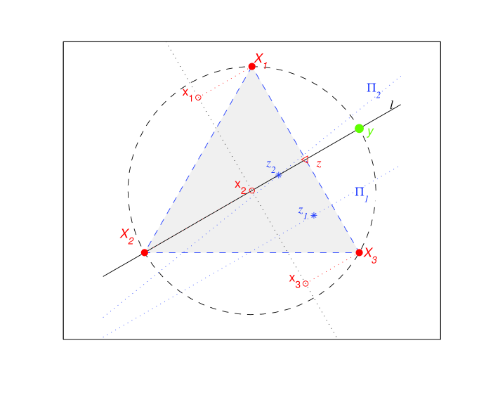
The key step of Theorem 1 is to locate the new maximizers of Tukey’s halfspace depth function after adding $\mathcal{Y}^{m}$ to $\mathcal{X}^{n}$. Considering the $\mathbb{A}_{\textbf{\emph{u}}}$-projections of the original observations is a helpful way to achieve this goal of identifying the maximizer. It turns out that the point z on the boundary of $\textbf{cov}(\mathcal{X}^{n})$, that determines a unit vector $\textbf{\emph{u}}_{\textbf{\emph{y}}}=(\textbf{\emph{y}}-\textbf{\emph{z}})/\|\textbf{\emph{y}}-\textbf{\emph{z}}\|$ such that the $\mathbb{A}_{\textbf{\emph{u}}_{\textbf{\emph{y}}}}$-projections of y lies in the interior of $\mathcal{M}(\mathbf{X}_{\textbf{\emph{u}}_{\textbf{\emph{y}}}}^{n})$, plays a key role in the whole proof of Theorem 1.

To gain an intuitive understanding of this, we provide a 2-dimensional illustration in Figure 1, where $X_{1},X_{2},X_{3}$ denote the data points, and $\mathbf{x}_{1},\mathbf{x}_{2},\mathbf{x}_{3}$ the corresponding $\mathbb{A}_{\textbf{\emph{u}}_{\textbf{\emph{y}}}}$-projections. When $m=1$, the Tukey depth of the point z with respect to $\mathcal{X}^{n}\cup\mathcal{Y}^{m}=\{X_{1},X_{2},X_{3},\textbf{\emph{y}}\}$ is clearly $1/2$, greater than that of any point outside the convex hull of $\{X_{1},X_{2},X_{3}\}$. On the other hand, the depth of any $\textbf{\emph{x}}\in\textbf{cov}(\mathcal{X}^{n})\setminus\{\textbf{\emph{z}}\}$ is smaller than $1/2$ (see $\textbf{\emph{z}}_{1}$, $\textbf{\emph{z}}_{2}$ for example).

Figure 1: Shown is a 2-dimensional illustration for Theorem 1.

Note that when $\textbf{\emph{u}}_{0}\in\mathcal{S}^{d-1}$ satisfies (1), $\mathbf{X}_{\textbf{\emph{u}}_{0}}^{n}$ is in general position from Lemma 1. Hence, relying on Proposition 2.3 in DG92, Theorem 1 in Liu et al. (2015) and Theorem 1 above, we can easily obtain the following proposition. Since the proof is trivial, we omit it here.

Proposition 1. Suppose $\mathcal{X}^{n}$ is in general position. When $d\geq 2$, the FSBP of Tukey’s halfspace median $T^{*}$ satisfies that

$$\frac{\left\lceil\frac{n}{d}\right\rceil}{n+\left\lceil\frac{n}{d}\right\rceil}\leq\varepsilon(T^{*},\mathcal{X}^{n})\leq\left\{\begin{array}[]{lcl}\frac{\lfloor\frac{n-d+3}{2}\rfloor}{n+\lfloor\frac{n-d+3}{2}\rfloor},&&\text{if }\exists\textbf{\emph{u}}_{0}\in\mathcal{S}^{d-1}\text{ satisfying }\eqref{eqnu0},\\ &&\text{ and }\mathcal{M}(\mathbf{X}_{\textbf{\emph{u}}_{0}}^{n})\text{ is singleton},\\ &&\\ \frac{\lfloor\frac{n-d+2}{2}\rfloor}{n+\lfloor\frac{n-d+2}{2}\rfloor},&&\text{otherwise}.\\ \end{array}\right.$$

Remark 3.2. For $d=2$, (a) when $n$ is even, $\mathcal{M}(\mathbf{X}_{\textbf{\emph{u}}_{0}}^{n})$ is of affine dimension 1, we have $\lfloor\frac{n-d+2}{2}\rfloor=\lceil\frac{n}{2}\rceil$; (b) when $n$ is odd, $\mathcal{M}(\mathbf{X}_{\textbf{\emph{u}}_{0}}^{n})$ is singleton, we have $\lfloor\frac{n-d+3}{2}\rfloor=\lceil\frac{n}{2}\rceil$. Both scenarios indicate that $\varepsilon(T^{*},\mathcal{X}^{n})$ attains the upper bound $\lceil\frac{n}{2}\rceil/(n+\lceil\frac{n}{2}\rceil)$.

(a) The scatter plot of the data set.

(b) The first scenario of the $\mathbb{A}_{u}$-projections.

(c) The second scenario of the $\mathbb{A}_{\textbf{\emph{u}}}$-projections.

(d) The third scenario of the $\mathbb{A}_{\textbf{\emph{u}}}$-projections.

(e) The fourth scenario of the $\mathbb{A}_{\textbf{\emph{u}}}$-projections.

Figure 2: Shown is an example for the upper bound for Proposition 1.

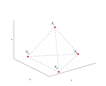
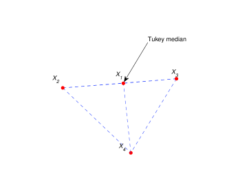
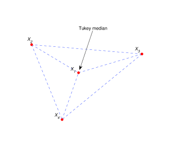
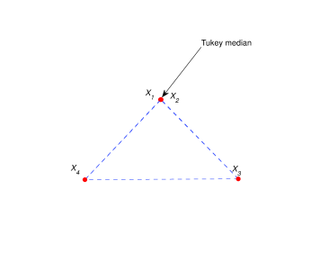
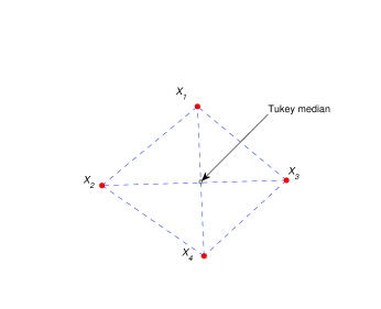
Both the upper and low bound given in Proposition 1 is attained if the data set is strategically choosed. Let’s first see an illustration for the upper bound. The data points are plotted in 2(a). The scatter plot of the $\mathbb{A}_{\textbf{\emph{u}}}$-projections of this data set has four scenarios, though, as shown in Figures 2(b)-2(e). The maximum Tukey depth $\lambda^{*}(\mathbf{X}_{\textbf{\emph{u}}}^{n})$ is equal to $1/2$ for any $\textbf{\emph{u}}\in\mathcal{S}^{d-1}$, nevertheless. Clearly, $1/2=\left\lfloor\frac{4-3+3}{2}\right\rfloor/4$, and hence $\varepsilon(T^{*},\mathcal{X}^{n})=1/3$ attains the upper bound given Proposition 1 for this data set.

(a) The scatter plot of the original data set.

(b) The scatter plot of the $\mathbb{A}_{\textbf{\emph{u}}}$-projections.

Figure 3: Shown is an example for the low bound for Proposition 1.

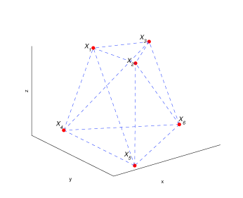
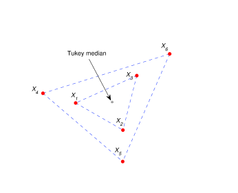
As to the low bound, we have an example shown in Figure 3(a). Since we can find a u such that the $\mathbb{A}_{\textbf{\emph{u}}}$-projections of the original data set is a data set of points at the vertices of a collection of nested simplices; See Figure 3(b). The maximum Tukey depth with respect to these projections is only $2/6=1/d$ when $d=3$. Hence, similar to DG92, the low bound of Proposition 1 is also attained, with $\varepsilon(T^{*},\mathcal{X}^{n})=1/4$ for this example.

Compared to the asymptotic result $1/3$, Proposition 1 indicates that the dimension $d$ indeed affects the finite sample breakdown point robustness of Tukey’s halfspace median. In detail, when $d$ increases, $\varepsilon(T^{*},\mathcal{X}^{n})$ tends to decrease for fixed $n$. In fact, the true FSBP of Tukey’s halfspace median may be less than $1/3$ under the IGP assumption, and this gap may be very great in practice when $d$ is large relative to $n$.

4 Concluding remarks

In the literature, it has long been a open question as to the exact finite sample breakdown point of Tukey’s halfspace median. In this paper, we resolved this question through taking account of the $\mathbb{A}_{\textbf{\emph{u}}}$-projections of the original observations when they are in general position. A precise result was provided for fixed sample size $n$. The current results revealed that, complimenting the asymptotic result (1/3) obtained by DG92, the finite sample breakdown point robustness of HM may be affected greatly by the dimension $d$, especially when $d$ is large relative to $n$. Since many offsprings, such as regression depth and multiple output regression, originated directly from Tukey’s halfspace depth function with the finite sample breakdown point of their median-like estimators unsolved, we wish that the developed results have the potential to facilitate the investigation of their finite sample breakdown point robustness.

Observe that $\inf_{\textbf{\emph{u}}\in\mathcal{S}^{d-1}}\lambda^{*}(\mathbf{X}_{\textbf{\emph{u}}}^{n})$ involves an infinite number of maximum Tukey depths $\lambda^{*}(\mathbf{X}_{\textbf{\emph{u}}}^{n})$. It computation is not trivial, and would be very time-consuming. Quite fortunately, there has been much progress in the computation of Tukey’s halfspace median and its related depth; See, for example, Rousseeuw and Ruts (1998), Struyf and Rousseeuw (2000) and Liu et al. (2015) and reference therein.

References

- Adrover and Yohai (2002) Adrover, J., Yohai, V., 2002. Projection estimates of multivariate location, Ann. Statist. 30, 1760-1781
- Chen (1995) Chen, Z., 1995. Robustness of the half-space median. Journal of statistical planning and inference, 46(2), 175-181.
- Chen and Tyler (2002) Chen, Z., Tyler, D.E., 2002. The influence function and maximum bias of Tukey s median. Ann. Statist. 30, 1737-1759.
- Donoho (1982) Donoho, D.L., 1982. Breakdown properties of multivariate location estimators. Ph.D. Qualifying Paper. Dept. Statistics, Harvard University.
- Donoho and Huber (1983) Donoho, D.L., Huber, P.J., 1983. The notion of breakdown point. In A Festschrift for Erich L. Lehmann (P.J. Bickel, K.A., Doksum and J.L. Hodges, Jr. eds.) 157-184. Wadsworth, Belmont, CA.
- Donoho and Gasko (1992) Donoho, D.L., Gasko, M., 1992. Breakdown properties of location estimates based on halfspace depth and projected outlyingness. Ann. Statist. 20, 1808-1827.
- Donoho and Huber (1983) Donoho, D.L., Huber, P.J., 1983. The notion of breakdown point. In: Bickel, P.J., Doksum, K.A., Hodges Jr., J.L. (Eds.), A Festschrift foe Erich L. Lehmann. Wadsworth, Belmont, CA, pp. 157-184.
- Dyckerhoff and Mozharovskyi (2016) Dyckerhoff, R., Mozharovskyi, P., 2016. Exact computation of the halfspace depth. Comput. Statist. Data Anal., 98, 19-30.
- Hampel (1971) Hampel, F.R., 1971. A general qualitative definition of robustness. Ann. Math. Statist. 42, 1887-1896.
- Hallin et al. (2010) Hallin, M., Paindaveine, D., Šiman, M., 2010. Multivariate quantiles and multiple-output regression quantiles: From optimization to halfspace depth. Ann. Statist. 38, 635-669.
- Hodges (1967) Hodges, J.L., 1967. Efficiency in normal samples and tolerance of extreme values for some estimates of location. Proceedings of the Fifth Berkeley Symposium on Mathematical Statistics and Probability, 1, 163-168.
- Huber (1964) Huber, P.J., 1964. Robust Estimation of a Location Parameter, Ann. Math. Statist. 35, 73-101.
- Huber (1981) Huber, P.J., 1981. Robust statisitcs. Wiley, New York.
- Liu and Singh (1992) Liu, R. Y., Singh, K., 1992. Ordering directional data: concepts of data depth on circles and spheres. The Annals of Statistics, 1468-1484.
- Liu et al. (2013) Liu, X.H., Zuo, Y.J., Wang, Z.Z., 2013. Exactly computing bivariate projection depth median and contours. Comput. Statist. Data Anal. 60, 1-11.
- Liu et al. (2015) Liu, X.H., Luo, S.H., Zuo, Y.J., 2015. Some results on the computing of Tukey’s halfspace median. Mimeo.
- Lopuhaä and Rousseeuw (1991) Lopuhaä, H.P., Rousseeuw, P.J., 1991. Breakdown Points of Affine Equivariant Estimators of Multivariate Location and Covariance Matrices. Ann. Statist. 19, 229-248.
- López-Pintado and Romo (2009) López-Pintado, S., Romo, J., 2009. On the Concept of Depth for Functional Data. J. Amer. Statist. Assoc. 104, 718-734.
- Mizera (2002) Mizera, I. 2002. On depth and deep points: a calculus. Annals of Statistics, 1681-1736.
- Mosler et al. (2009) Mosler, K., Lange, T., Bazovkin, P., 2009. Computing zonoid trimmed regions of dimension . Comput. Statist. Data Anal. 53, 2500-2510.
- Oja (1983) Oja, H., 1983. Descriptive statistics for multivariate distributions. Statist. Probab. Lett. 1, 327-332.
- Paindaveine and Šiman (2011) Paindaveine, D., Šiman, M., 2011. On directional multiple-output quantile regression. J. Multivariate Anal. 102, 193-392.
- Rousseeuw and Hubert (1999) Rousseeuw, P.J., Hubert, M., 1999. Regression depth (with discussion). J. Amer. Statist. Assoc. 94, 388-433.
- Rousseeuw and Ruts (1998) Rousseeuw, P. J., Ruts, I. 1998. Constructing the bivariate Tukey median. Statistica Sinica, 827-839.
- Struyf and Rousseeuw (2000) Struyf, A., Rousseeuw, P.J. 2000. High-dimensional computation of the deepest location. Comput. Statist. Data Anal., 34(4), 415-426.
- Tukey (1975) Tukey, J.W., 1975. Mathematics and the picturing of data. In Proceedings of the International Congress of Mathematicians, 523-531. Cana. Math. Congress, Montreal.
- Weber (1909) Weber, A., 1909. Uber den Standort der Industrien, Tubingen. In: Alfred Weber s Theory of Location of Industries, University of Chicago Press. English translation by Freidrich, C.J. (1929).
- Zuo (2001) Zuo, Y., 2001. Some quantitative relationships between two types of finite sample breakdown point. Stat. Probab. Lett. 51, 369-375
- Zuo and Serfling (2000) Zuo, Y.J., Serfling, R., 2000a. General notions of statistical depth function. Ann. Statist. 28, 461-482.