Turbulent mixing and a generalized
phase transition in shear-thickening fluids

Abstract

This paper presents a new theory of turbulent mixing in stirred reactors. The degree of homogeneity of a mixed fluid may be characterized by (among other features) Kolmogorov’s microscale, $\lambda$. The smaller its value, the better the homogeneity. According to Kolmogorov, $\lambda$ scales inversely with the fourth root of the energy flux applied in the stirring process, $\varepsilon$. The higher $\varepsilon$, the smaller $\lambda$, and the better the homogeneity in the reactor. This is true for Newtonian fluids. In non-Newtonian fluids the situation is different. For instance, in shear-thickening fluids it is plausible that high shear rates thicken the fluid and might strangle the mixing. The internal interactions between different fluid-mechanical and colloidal variables are subtle, namely due to the (until recently) very limited understanding of turbulence.
   Starting from a qualitatively new turbulence theory for inviscid fluids [Baumert(2013)], giving e.g. Karman’s constant as $1/\sqrt{2\,\pi}=0.40$ [[, Princeton’s superpipe gives 0.40$\pm 0.02$,]]baileyetal2014, we generalize this approach to the case of viscous fluids and derive equations which in the steady state exhibit two solutions. One solution branch describes a state of good mixing, the other strangled turbulence. The physical system cannot be in two different steady states at the same time. But it is physically admissible to switch between the two steady states by non-stationary transitions, maybe in a chaotic fashion.

Keywords: Turbulence, kinematic viscosity, eddy viscosity, colloidal systems, dispersions, shear-thickening, mixing, stirring, reactor, non-Newtonian fluid, Kolmogorov scale, bifurcation

35pc Corresponding author: Dr. Helmut Z. Baumert,
IAMARIS, Bürgermeister-Jantzen-Str. 3, 19288 Ludwigslust, Germany (baumert@iamaris.org) Submitted for publication to Physica Scripta (IOP): 29 March, 2015

1 Introduction

Plausibility considerations

A mixer is a reactor wherein fluids are mixed with other fluids, with dry or liquid chemicals, heat or other so-called ‘scalars’. To that aim propellers, screws, raising bubbles or other technological stirring means and devices are applied. The near-field turbulence initiated by them is characterized by two parameters: a characteristic length scale and a characteristic time scale (or, equivalently, a corresponding wavenumber and a corresponding frequency). These two parameters may be tuned independently by modifying the geometry and the rotation rate of the device (the bubble-release frequency in bubble or convective mixing).

If the operator of a mixer wishes a higher degree of homogeneity then he is inclined to increase the energy spend for mixing by increasing the rotation rate, the geometric parameters of the propeller, or both. For Newtonian fluids this is a reasonable strategy. However, in shear-thickening fluids it is plausible that with an increase of the forcing one might contribute to thickening which in the extreme strangles mixing until breakdown of turbulence. Here much depends on details, i.e. how one increases the stirring power, by geometric means, by the rotation rate, or by both.

As mixing and dispersion are fundamental technological steps in nearly all industries and connected with huge financial fluxes if considered for the globe, this circle of questions deserves attention.

Historical remarks

Whereas the arts of hydraulics including the phenomenology of eddying flows and vortices are well known at least for about $2.4\times 10^{3}$ years, back to e.g. the ‘hydraulic empires’ of Nofretete and Echnaton, the mathematical science of dynamic fluid motions emerged ’just recently’: in idealized, purely geometric form by Leonhard Euler (1707 - 1783), supplemented somewhat later with frictional aspects by Claude-Louis Navier and George Stokes. The theory of vortices and circulation was more explicitely elaborated about 30 years later by Herrmann von Helmholtz and William Thomson (Lord Kelvin), and later came Osborne Reynolds, Ludwig Prandtl, Theodore von Karman, Alexander A. Friedmann and Lev V. Keller with their specific innovations.

A systematic statistical treatment of turbulence was initiated by Geoffrey I. Taylor and, in form of spectral considerations, by Andrej N. Kolmogorov. These attempts were more or less singular pieces, kept loosely together by semi-empirical scaling rules and similarity arguments. Great contributions in this respect stem here from Andrej S. Monin, Alexander Obukhov, Rostislav V. Osmidov, Chuck van Atta and Stephen Thorpe.

With the advent of sufficiently powerful computers the focus moved towards so-called two-equation turbulence models. Major authors are David C. Wilcox, George L. Mellor, Tetsuji Yamada, and Wolfgang Rodi. The overwhelming number of turbulence theories in the above sense were elaborated for Newtonian fluids (and gases) wherein kinematic viscosity is more or less constant in larger elements of space and time and not dependent neither on the state of the fluid motion nor on external forces, nor on time.

Smart fluids / colloidal systems

Today so-called smart fluids become increasingly relevant in various industries, from medicine over small-scale bio-technology to construction engineering, waste-water treatment and defence. The central property of a smart fluid is its kinematic viscosity, which may explicitely depend on time or not, which may be tuned by shear or light, by electric or magnetic fields like in magneto-rheological fluids.

As their kinematic viscosity is not a constant, smart fluids have always non-Newtonian character. They all are at least 2-phase systems, whereas the – at least one – dispersed phase is mostly nanoscopic (i.e., less than 100 nm diameter) in size. Hence these are colloidal systems, either colloidal dispersions (the dispersed phase being a solid) or emulsions (the dispersions being a liquid). In contrast to wide-spread assumptions, such colloidal systems exhibit complex structures. I.e., the dispersed phase is not statistically evenly distributed, but highly structured [Wessling(1993)]. This is due to the thermodynamically non-equilibrium character of such colloidal dispersions / emulsion systems [Wessling(1991), Wessling(1995)].

As long as the flow of a non-Newtonian fluid or gas is laminar, the consequences of those external controls on the kinematic viscosity remain more or less predictable and no dispersion would be possible [Wessling(1995)]. This property is going to be changed when the flow becomes critical and eventually turbulent.

Even the Reynolds number in non-Newtonian fluids looses much of its classical meaning. Traditionally it is defined as the dimensionless ratio of inertial and viscous forces,

$$Re=\frac{U\times L}{\nu}$$ (1)

where $U$ [m s^-1] is a velocity scale for the mean flow, $L$ [m] a characteristic length scale (e.g. a distance from a solid wall or body) and $\nu$ is the kinematic viscosity [m${}^{2}\,$s^-1]. This means that $Re$ depends linearly on the state of flow via the velocity, $U$. However, if also $\nu$ depends on the flow state then things become more difficult.

Relatively simple cases of smart fluids are the so-called shear-thickening (dilatant) and the shear-thinning (pseudoplastic) fluids. In the former case viscosity increases with increasing shear rate so that the fluid becomes ‘thicker’. The most prominent example is the fluid in body armor wests of policemen. Certain water-sand mixtures may behave in similar form. Prominent examples for pseudoplastic fluids are lava, blood and whipped cream. Also the notorious quicksand is an example for a shear-thinning material.

In all these cases the turbulent state of those fluids – if at all – is understood only in an empirical sense.

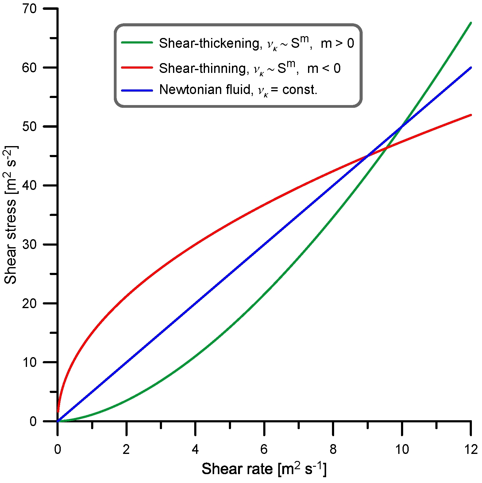
Figure 1: Examples of shear behavior in a shear-thickening (green, m=0.65), a shear-thinning (red) and a Newtonian fluid.

The kinematic viscosity of many non-Newtonian fluids may be described as a power-law function of local shear rate, $S$, by the following slightly generalized Ostwald-de Waehle ansatz, wherein $\nu_{0}=\nu_{0}(T)$ and $\gamma=\gamma(T)$ are (generally temperature-dependent) empirical parameters:

$$\nu=\nu_{0}+\gamma\times({S}/{S_{*}})^{m}\,.$$ (2)

Fig. 1 shows three example fluids with (not completely fictive) parameters like $\gamma=10^{-6}$ m² s^-1, $S_{*}=0.19$ s^-1 (Hz), $\nu_{0}=0.43$ m² s^-1, and with $m=\{-0.5;+0.65;+1.5\}$.

In the following we exclusively deal with shear-thickening fluids ($m>0$) and use the notion of turbulence in a narrow sense defined later. Nevertheless the theoretical foundations cover a broader range of applications than only the shear-thickening case.

Theoretical foundation

This paper rests essentially on [Baumert(2013)] who demonstrated that the turbulent viscosity, $\nu_{t}$ [m² s^-1], scaling linearly with turbulent diffusivity, $\mu_{t}$ [m² s^-1], may be written as follows,

$$\nu_{t}=\frac{\cal K}{\pi\,\Omega}$$ (3)

where $\cal K$ is turbulent kinetic energy in the narrow sense, TKE [m² s^-2], $\Omega$ is the r.m.s. turbulent vorticity [s^-1] (a relative of enstrophy) and $\pi$ is the dimensionless circle number. This formula results from a stochastic-geometric theory of inviscid turbulence wherein turbulent eddies are taken as singular solutions of the Euler equation and thus as particles (vortex-tubes dipoles) moving in a stochastic fashion – just like molecules in Einstein’s theory of Brownian motion – slightly generalized in form of Fokker-Planck equations wtih generation and dissipation terms. Another result of this theory is the Karman constant as

$${\ae}=1{/}\sqrt{2\pi}=0.40\;.$$ (4)

[[, A recent study based on the Princeton Superpipe gave $0.40\pm 0.02$, see]]baileyetal2014.

2 Inviscid and viscous spectra

The major length scales

Wavenumber spectra of developed viscous turbulence exhibit two distuingished scales: the larger, so-called energy-containing scale which depends on the forcing mechanism, $\Lambda$, and the smaller Kolmogorov scale, $\lambda\ll\Lambda$ , which is related with the kinematic viscosity, $\nu$:

$$\lambda=\left(\frac{\nu^{3}}{\varepsilon}\right)^{1/4}\;.$$ (5)

Here $\varepsilon$ [m² s^-3] is the total turbulent dissipation rate of TKE, and $\nu$ [m² s^-1] is the kinematic viscosity. Obviously, if $\nu\rightarrow 0$, also $\lambda\rightarrow 0$.

The energy-containing turbulent scale, $\Lambda$, has been derived on theoretical grounds as follows [Baumert(2013)],

$$\Lambda=\frac{\sqrt{{\cal K}/\pi}}{\Omega}\,.$$ (6)

This scale is only indirectly influenced by viscosity.

Figure 2: Inviscid (dashed) and viscous (full) spectra of kinetic-energy fluctuations, dimensionless. $\kappa_{\Lambda}=2\,\pi$ and $\kappa_{\lambda}=2\,\pi\,{\Lambda}/\lambda$ denote the dimensionless forms of the energy-containing and the Kolmogorov wavenumber, respectively.

Wavenumber spectra

For a better understand of our approach we look at Fig. 2. It exhibits a real-world viscous spectrum (full) and an idealized spectrum of inviscid turbulence (dashed) discussed in [Baumert(2013)]. With the dimensionless wave number $\kappa=k\times{\Lambda}$ [Pope(2000), eqn. 6.246, p. 232] it reads as follows,

$${\cal E}(\kappa)=\frac{E(\kappa)}{\varepsilon^{2/3}{\Lambda}^{5/3}}={C}\times f_{\Lambda}(\kappa)\times\kappa^{-5/3}\times f_{\lambda}(\kappa,\rho)$$ (7)

where

$$\rho={\Lambda}/\lambda.$$ (8)

$\rho$ is taken below as a rough proxy of the Reynols number.

$C$ in (7) is a so-called universal Kolmogorov constant for the wavenumber spectrum of turbulence. It has been derived theoretically as follows [Baumert(2013)]:

$$C=\frac{1}{3}(4\pi)^{2/3}=1.80\,.$$ (9)

In (7), $f_{\Lambda}(\kappa)$ describes the low-wavenumber, high-energy interval following Karman’s spectral model [[, loc. cit.]p. 747]pope2000. $f_{\lambda}(\kappa,\rho)$ denotes the so-called dissipation region wherein the smallest eddy motions are becoming laminar [[, for details see p. 232, 233 in]]pope2000:

$$f_{L}(\kappa)=\left(\frac{\kappa}{\sqrt{\kappa^{2}+c_{L}}}\right)^{17/3}$$ (10)

and

$$f_{\lambda}(\kappa,\rho)=\exp\left[-\beta\left(\left[\left(\frac{\kappa}{\rho}\right)^{4}+c_{\lambda}^{4}\right]^{1/4}-c_{\lambda}\right)\right]\,.$$ (11)

[[, The exponential ansatz for the dissipation region is in a simpler form due to Kraichnan (1959), loc. cit.]]pope2000.

Figure 3: Spectra of kinetic-energy fluctuations for the Reynolds-number proxy $Re=L/\lambda$ decreasing from the upper right curve with $Re=\infty$ down to the lower left with $Re=10$. We see that the area below Kolmogorov’s $\kappa^{-5/3}$ inertial subrange not only shrinks quantitatively with decreasing $Re$. It even vanishes completely, indicating the transition from the turbulent to the laminar state.

3 Turbulence in the narrow sense
and other chaotic motions

In the present paper we understand the notion turbulence in a specific narrow sense and separate it from other forms of chaotic fluid motions. We distinguish three regions of the kinetic-energy wavenumber spectrum. We namely interprete Kolmogorov’s inertial subrange in the interval [$\kappa_{\Lambda},\kappa_{\lambda}$] as turbulence in the narrow sense and the rest of the spectrum simply as other forms of chaotic fluid motions which mix only weakly.

We differentiate between the following three wavenumber intervals:

• $\kappa\in[0,\kappa_{\Lambda}]$: weakly mixing Karman range,

• $\kappa\in[\kappa_{\lambda},\kappa_{\Lambda}]$: intensely mixing inertial
  subrange of Kolmogorov,

• $\kappa\in[\kappa_{\lambda},\infty]$: weakly mixing Kraichnan region.

Arguments for (ii) are given in the next section.

Regarding mixing of momentum in the sense of (3), only the Kolmogorov range matters which in the inviscid case ($k_{\lambda}\rightarrow\infty$) extends from the energy-containing scale, $k_{\Lambda}$, until $k_{\lambda}=\infty$ so that

$${\cal K}=\int_{k_{\Lambda}}^{\infty}E(k)\,dk=C\times\varepsilon^{2/3}\times\int_{k_{\Lambda}}^{\infty}\frac{dk}{k^{5/3}}\;.$$ (12)

This last integral gives together with (6) a simple analytical result:

$${\cal K}=C\times\frac{3}{2}\times\left(\frac{\varepsilon\,\Lambda}{2\pi}\right)^{2/3}\;.$$ (13)

This result has successfully been tested against high-$Re$ turbulence observations [[]Fig. 6]baumert2013.

Now we apply this approach to viscous turbulence and write

$${\cal K}=\int_{k_{\Lambda}}^{k_{\lambda}}E(k)\,dk\;.$$ (14)

Clearly, (12) is a special case of (14).

(14) is analytically integrable and gives the following:

$${\cal K}=C\times\frac{3}{2}\times\left(\frac{\varepsilon}{2\pi}\right)^{2/3}\times\left[{\Lambda}^{2/3}-{\lambda}^{2/3}\right].$$ (15)

Due to (5), a kinematic viscosity $\nu$ increasing without bounds gives an increasing $\lambda$ until $\lambda=\Lambda$ at which point according to (15) TKE vanishes. This means that turbulence in the narrow sense (Kolmogorov’s inertial subrange) disappears and chaotic laminar motions of the now joined Karman-Kraichnan range remain. If ${\cal K}=0$, then eddy viscosity $\nu_{t}$ via (3) and consequently also eddy diffusivity $\mu_{t}$ vanish accordingly.

4 Mixing within and outside the Kolmogorov subrange

Our view of Kolmogorov’s inertial subrange has been filled with life through reports on a series of numerical simulation studies [Herrmann(1990), Herrmann et al.(1990)Herrmann, Mantica, and Bessis, Manna and Herrmann(1991)] wherein spectra of space-filling bearing were shown to correspond closely to Kolmogorov’s 5/3 spectral law. A space-filling bearing is identical with the densest non-overlapping (Apollonian) circle packing in a plane, with side condition that the circles are pointwise in contact but able to rotate freely, without friction or slipping [[, a devil s gear sensu ]]poeppe04. The contact condition for two different wheels with indices 1 and 2 of the gear reads

$$\omega_{1}\times r_{1}=\omega_{2}\times r_{2}.$$ (16)

A devil’s gear forms spontaneously when vortex dipoles collide. Those dipoles move with their inctrinsic velocity governed by their given radius $r$ and rotation speed $\omega$ [Baumert(2013)]. When they collide they are either scattered or annihilated. The latter case is realized in form of a dissipative patch wherein all scales $>0$ are frictionless except the scale zero where all the dissipation takes place. Because a dissipative patch in form of a devil’s gear remains at rest, scatter motions scaling with the intrinsic parameters $r,\omega$ are the only source of place changes and thus of mixing [Baumert(2013)].

Although in these patches scalar mixing takes also place, the bulk of it is due to the place changes of dipoles. Hoever, momentum mixing is exclusively due to place changes of the dipoles. This is the deeper reason why generally $\mu_{t}>\nu_{t}$. I.e. the turbulent Prandtl number $\sigma=\nu_{t}/\mu_{t}$ is generally less than unity.

5 Balance equations for $\cal K$ and $\Omega$
in a homgeneously stirred reactor

General

The dynamic balances of $\cal K$ and $\Omega$ in a homgeneously stirred reactor are given as follows [Baumert(2013)]:

$$\frac{d\cal K}{dt} = \nu_{t}\,{S}^{2}-\varepsilon_{h}-\varepsilon_{b}\,,$$ (17)

$$\frac{d\Omega}{dt} = \frac{1}{\pi}\left(\frac{1}{2}{S}^{2}-\Omega^{2}\right).$$ (18)

Here $\nu_{t}$ is the eddy viscosity given by (3), $S=\langle S_{e}^{2}\rangle^{1/2}$ is the (steady) r.m.s. effective shear rate, $\varepsilon_{h}={\cal K}\,\Omega/\pi$ [Baumert(2005)] is the dissipation rate within the bulk volume, and $\varepsilon_{b}$ is the bulk dissipation within the boundary layers (walls etc.) of the reactor.

In the following we denote steady state values ($d{\cal K}/dt=d\Omega/dt=0$) by an overbar. In particular we have

$$\overline{\varepsilon}_{b}=\overline{\varepsilon}_{h}=\frac{\overline{\cal K}\,\overline{\Omega}}{\pi}\,,$$ (19)

fully indepenent on the forcing ${S}$. Whereas the steady-state case of the dynamic energy balance (17) is useless for the following, the steady-state r.m.s. vorticity balance finds application further below:

$$\overline{\Omega}={S}/\sqrt{2}\,,$$ (20)

Steady state

Until now we have no equation yet which gives us the size of Kolmogorov’s microscale, $\lambda$. It is derived now, based on the above results and thoughts. We begin with (15) and replace there the homogeneous volume dissipation rate via $\overline{\varepsilon}=\overline{\varepsilon}_{h}=\overline{\cal K}\;\overline{\Omega}/\pi$ and find with (20) the following relation for the steady-state turbulent kinetic energy in the reactor:

$$\overline{\cal K} = \alpha_{1}\times\overline{S}^{2}\times\left[{\Lambda}^{2/3}-{\overline{\lambda}}^{2/3}\right]^{3}\,,$$ (21)

$$\alpha_{1} = (2\pi)^{-2}\;\;\;=\;\;\;0.0253.$$ (22)

This result allows to reformulate the steady-state eddy viscosity (3) in the reactor as follows:

$$\overline{\nu}_{t} = \frac{\overline{\cal K}}{\pi\,\overline{\Omega}}\;\;=\;\;\alpha_{2}\times{S}\times\left[{\Lambda}^{2/3}-\overline{\lambda}^{2/3}\right]^{3},$$ (23)

$$\alpha_{2} = 2^{-3/2}\times\pi^{-3}\;\;\;=\;\;\;0.0114.$$ (24)

Analogously we may derive the steady-state TKE dissipation rate in the reactor as

$$\overline{\varepsilon} = \frac{\overline{\cal K}\,\overline{\Omega}}{\pi}\;\;=\;\;\alpha_{3}\times{S}^{3}\times\left[{\Lambda}^{2/3}-\overline{\lambda}^{2/3}\right]^{3},$$ (25)

$$\alpha_{3} = 2^{-5/2}\times\pi^{-3}\;\;\;=\;\;\;0.00570.$$ (26)

6 Microscale bifurcation

Governing equation

We now consider according to (5) the steady-state microscale, $\overline{\lambda}$ and replace therein $\varepsilon$ with the reactor’s steady-state value (25):

$$\overline{\lambda}=\left(\frac{\overline{\nu}^{3}}{\overline{\varepsilon}}\right)^{1/4}=\alpha_{4}\times\left(\frac{\overline{\nu}/{S}}{\Lambda^{2/3}-\overline{\lambda}^{2/3}}\right)^{3/4},$$ (27)

$$\alpha_{4}=\alpha_{3}^{-1/4}=1.1509\,.$$ (28)

For an easy treatment of (27) we multiply both sides with $\left[\Lambda^{2/3}-\overline{\lambda}^{2/3}\right]^{3/4}$ and get with some algebra and using the abbreviation $\xi=\overline{\lambda}^{2}$ the following working equation:

$$(\xi\,\Lambda)^{2/3}=\xi+\alpha_{4}^{4/3}\,\overline{\nu}/{S}\,.$$ (29)

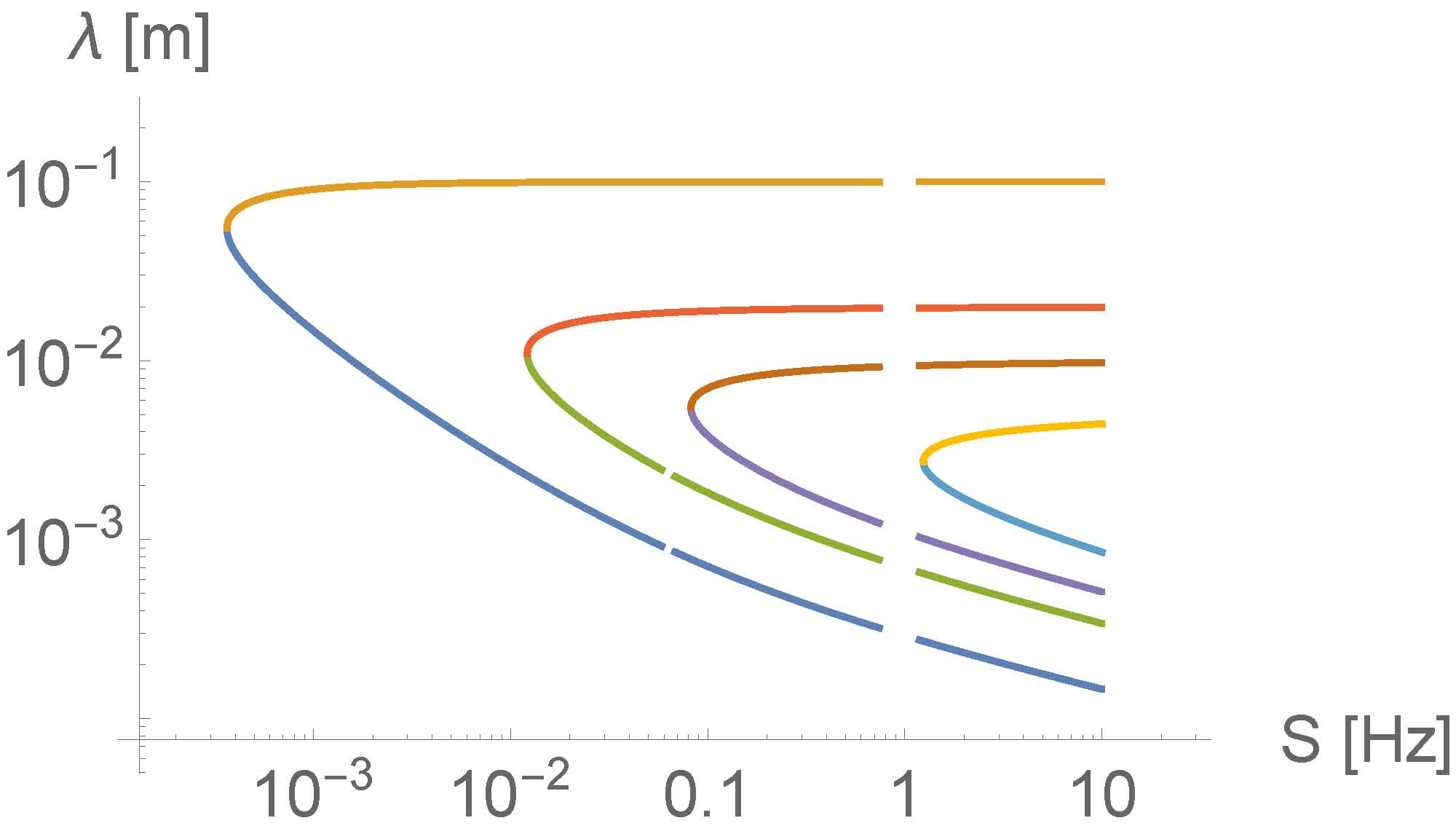
Figure 4: Valid steady-state combinations of forcing parameters $\Lambda,\lambda$. Note that always two states are possible, the upper branch without turbulence in the narrow sense, and the lower branch with a developed Kolmogorov spectrum with the property $\lambda\ll\Lambda$. The forcing length scales are here $\Lambda$ = 10 cm, 2 cm, 1 cm, 5 mm, respectively, from outside to inside.

Figure 5: Similar to Fig. 4 but instead of $\lambda$ the scale ratio $1/\rho=\lambda/\Lambda$ is shown. $\rho$ proper is a proxy for the Reynolds number. $\rho=1$ means that the Kolmogorov scale equals the energy-containing scale so that the highly mixing inertial subrange of the fluctuation spectrum vanishes and mixing breaks more or less down. The forcing length scales are here again $\Lambda$ = 10 cm, 2 cm, 1 cm, 5 mm (from outside to inside). Note that the second horizontal line is situated at $\lambda/\Lambda\approx 0.53$ and labels the border between the upper and lower solution branches of (29).

Physical interpretation

The meaning of (27) is most easily understood by highlighting input and output variables and assuming mechanical stirring:

• The shear frequency, $\mathbf{S}$, is controlled by the rotation speed of (e.g.) the propeller(s) used to stir the reactor. I.e. for the solution of (27), $\mathbf{S}$ is thus a given, prescribed input quantity.

• The turbulent length scale $\mathbf{\Lambda}$ is controlled by geometry (e.g. radius, length of stirring propeller etc.) and represents also a given, prescribed input quantity.

• The microscale $\overline{\mathbf{\lambda}}$ however is not given. It is the dynamic relaxation result of the forcing and thus an output quantity.

As we see in Figures 4 and 5, for a given energy-containing length scale $\Lambda$ (i.e. along a chosen curve), each admissible shear value $S$ allows for two values of Kolmogorov’s microscale, $\lambda$:

• the upper value is associated with the strangling of turbulence due to the close proximity of $\lambda$ and $\Lambda$. This proximity leaves not enough space for a developed turbulence spectrum (in the narrow sense from above).

• The (mostly much) lower value is associated with a good mixing behavior of the stirred reactor. Unfortunately nature gives no stability guarantee for this state because there exists the “official” alternative of a strangeled spectrum – in agreement with the law. Some aspects are discussed in the next Section 7.

7 The full dynamic problem

Smart fluids, smart control?

We have shown in Section 6 that a reactor holding a shear-thickening fluid may attain two different steady states with respect to scalar mixing and turbulence. One of them mixes well, the other one does not.

Clearly the system cannot stay in both states at the same time. But non-steady transitions between them are physically possible and of practical interest. In Figures 4 and 5 these transitions occur ouside the computed curves.

Questions remain. E.g. how does the system choose, for a given set of initial conditions $\{{\cal K}_{0}$, $\Omega_{0}\}$ and forcing parameters $\{\Lambda,S\}$, between the two admissible steady states, and under which conditions (including initialization) transitions between them occur. Possibly smart fluids deserve smart means to keep them under control.

Relaxation of the “inner fluid”

Due to the inner structure of shear-thickening colloidal systems we have to expect that a viscosity according to (3) is never instantaneously realized. Dynamic adjustments to a new micro-mechanical state take certain relaxation steps. They are governed by the laws of irreversible thermodynamics [Wessling(1991), Wessling(1993), Wessling(1995)]. Therefore, to get a complete dynamic picture of the stirred fluid with our focus on learning how one of the two steady states is selected and how potential transitions between them are controllable, we actually have at least to augment the equation system (17, 18) by an additional equation for the dynamic relaxation of the kinematic viscosity (the “inner fluid”) against instantateous changes in the shear rate, $S=S(t)$.

These results now quantitatively explain the previously only empirically observed non-Newtonian viscosity due to structure build-up and -breakdown in colloidal systems under different shear conditions. They are fully in line with thermodynamical non-equilibrium character of colloidal systems: the result of chaotic dispersion processes (which are empirically known not to be easy to control and having quite often unexpected results which require intensive studies of the process parameters until finally in mass production reproducible results can be achieved)

Coda

At least in the present moment we have no detailed knowledge of the inner relaxation behavior of our test fluid. Therefore we have to apply here the most simple ansatz – linear or “first order” relaxation (“nudging”). We augment (17, 18) as follows,

$$\frac{d\nu}{dt} = \frac{1}{\tau}\left(\tilde{\nu}-\nu\right).$$ (30)

This equation describes the inner microscopic-dynamic relaxation of $\nu=\nu(t)$ wherein $\tilde{\nu}$ is the steady-state value of the kinematic viscosity and known from above as the Ostwald-de Waehle relation,

$$\tilde{\nu}=\nu_{0}+\gamma\times({S}/{S_{*}})^{m}\,.$$ (31)

Thus finally we have

$$\frac{d\nu}{dt} = \frac{1}{\tau}\left[\nu_{0}+\gamma\times\left(\frac{S}{S_{*}}\right)^{m}-\nu\right].$$ (32)

This is our first attempt to describe the effects of changes in nanoscopic structures of colloidal systems with respect to viscosity.

The value of $\tau$ can be measured in principle but is not yet available. Its value is important because its relation to intrinsic turbulent time scales matter. It is also not clear whether the linear ansatz is the correct one among the many other relaxation models. Further, although (17, 18, 32) form a closed dynamical problem, (17,18) are possibly not sufficiently representative for the state of strangled eddy viscosity [[, they have been derived for inviscid flows,]]baumert2013. These questions deserve specific experimental studies and further theoretical efforts.

Acknowledgements. HZB thanks Alexander J. Babchin in Tel Aviv for dropping hints on early fruitful efforts of Yakov Frenkel (1894 – 1952) towards a kinetic theory of liquids and certain generalized phase transitions.

References

- [Bailey et al.(2014)Bailey, Vallikivi, Hultmark, and Smits] Bailey, S. C. C., M. Vallikivi, M. Hultmark, and A. J. Smits, 2014: Estimating the value of von Karman’s constant in turbulent pipe flow. J. Fluid Mech., 749, 79 – 98, doi:dx.doi.org/10.1017/jfm.2014.208.
- [Baumert(2005)] Baumert, H. Z.: 2005, A novel two-equation turbulence closure for high Reynolds numbers. Part B: Spatially non-uniform conditions. Marine Turbulence: Theories, Observations and Models, H. Z. Baumert, J. H. Simpson, and J. Sündermann, eds., Cambridge University Press, Chapter 4, 31 – 43.
- [Baumert(2013)] Baumert, H. Z., 2013: Universal equations and constants of turbulent motion. Physica Scripta, T155, 014001 (12pp), doi:10.1088/0031-8949/2013/T155/014001.
- [Frenkel(1946)] Frenkel, Y., 1946: Kinetic Theory of Liquids. Clarendon Press, 1st engl. ed., 488 pp., russian ed. 1943, Kazan.
- [Herrmann(1990)] Herrmann, H. J.: 1990, Space-filling bearings. Correlation and Connectivity, H. E. Stanley and N. Ostrowsky, eds., Kluwer Academic Publ., 108 – 120.
- [Herrmann et al.(1990)Herrmann, Mantica, and Bessis] Herrmann, H. J., G. Mantica, and D. Bessis, 1990: Space-filling bearings. Phys. Rev. Letters, 65, 24 December, 3,223 – 3,226.
- [Manna and Herrmann(1991)] Manna, S. S. and H. J. Herrmann, 1991: Precise determination of the fractal dimensions of apollonian packing and space-filling bearings. Journal of Physics A, 24.
- [Pope(2000)] Pope, S. B., 2000: Turbulent flows. Cambridge U. Press, 771 pp.
- [Pöppe(2004)] Pöppe, C., 2004: Das Getriebe des Teufels. Spektrum d. Wiss., September, 104 – 109.
- [Wessling(1991)] Wessling, B., 1991: Dispersion hypothesis and non-equilibrium thermodynamics: key elements for a materials science of conductive polymers. A key to understanding polymer blends or other multiphase polymer systems. Synthetic metals, 45, 119 – 149.
- [Wessling(1993)] — 1993: Dissipative structure formation in collodial systems. Advanced Materials, 5, 300 – 305.
- [Wessling(1995)] — 1995: Critical shear rate – the instability reason for the creation of dissipative structures in polymers. Z. Phys. Chem., 191, 119 – 135.