Numerical Evaluation of the Bose-Ghost Propagator
in Minimal Landau Gauge on the Lattice

Abstract

We present numerical details of the evaluation of the so-called Bose-ghost propagator in lattice minimal Landau gauge, for the SU(2) case in four Euclidean dimensions. This quantity has been proposed as a carrier of the confining force in the Gribov-Zwanziger approach and, as such, its infrared behavior could be relevant for the understanding of color confinement in Yang-Mills theories. Also, its nonzero value can be interpreted as direct evidence of BRST-symmetry breaking, which is induced when restricting the functional measure to the first Gribov region $\Omega$. Our simulations are done for lattice volumes up to $120^{4}$ and for physical lattice extents up to $13.5$ fm. We investigate the infinite-volume and continuum limits.

I Introduction

Restriction of the functional integral to the first Gribov region $\Omega$ —given as the set of transverse gauge configurations for which the Faddeev-Popov (FP) matrix ${\cal M}$ is non-negative— defines the so-called minimal Landau gauge in Yang-Mills theories Gribov:1977wm . On the lattice, this gauge fixing is implemented by a minimization procedure (see e.g. Giusti:2001xf ), without the need to consider the addition of a nonlocal horizon-function term $\gamma^{4}S_{h}$ to the (Landau-gauge) action, as done in the Gribov-Zwanziger (GZ) approach in the continuum Zwanziger:1991ac . Let us recall that, in the GZ approach, the resulting (nonlocal) action may be localized by introducing auxiliary fields. Also, one can define for these fields a nilpotent BRST transformation (see e.g. Vandersickel:2012tz ), which is a simple extension of the usual perturbative BRST transformation that leaves the Yang-Mills action invariant in linear covariant gauge. However, it can be easily verified that, in the GZ case, this local BRST symmetry is broken by terms proportional to the Gribov parameter $\gamma$. More precisely, since a nonzero value of $\gamma$ is related to the restriction of the functional integration to $\Omega$, it is somewhat natural to expect a breaking of the perturbative BRST symmetry, as a direct consequence of the nonperturbative gauge-fixing. This issue has been investigated in several works (see e.g. Zwanziger:2009je ; Zwanziger:2010iz ; Maggiore:1993wq ; Zwanziger:1993dh ; vonSmekal:2008en ; Dudal:2008rm ; Baulieu:2008fy ; Dudal:2009xh ; Sorella:2009vt ; Kondo:2009qz ; Sorella:2010fs ; Capri:2010hb ; Dudal:2010hj ; Capri:2011wp ; Lavrov:2011wb ; Weber:2011nw ; Lavrov:2012gb ; Weber:2012vf ; Maas:2012ct ; Dudal:2012sb ; Capri:2013naa ; Schaden:2013ffa ; Reshetnyak:2013bga ; Brambilla:2014jmp ; Moshin:2014xka ; Capri:2014bsa ; Schaden:2014bea ; Reshetnyak:2014exa ; Capri:2015ixa ; Capri:2015nzw and references therein). The above interpretation is supported by the recent introduction of a nilpotent nonperturbative BRST transformation Capri:2015ixa ; Capri:2015nzw , which leaves the local GZ action invariant. The new symmetry is a simple modification of the usual BRST transformation $s$, by adding (for some of the fields) a nonlocal term proportional to the Gribov parameter $\gamma$, thus recovering the usual perturbative transformation $s$ when $\gamma$ is set to zero.

As indicated above, the Gribov parameter $\gamma$ is not introduced explicitly on the lattice, since in this case the restriction of gauge-configuration space to the region $\Omega$ is achieved directly by numerical minimization. Nevertheless, the breaking of the perturbative BRST symmetry induced by the GZ action may be investigated by the lattice computation of suitable observables, such as the so-called Bose-ghost propagator, which has been proposed as a carrier of the long-range confining force in minimal Landau gauge Zwanziger:2009je ; Furui:2009nj ; Zwanziger:2010iz . The first numerical evaluation of the Bose-ghost propagator in minimal Landau gauge was presented —for the SU(2) case in four space-time dimensions— in Refs. Cucchieri:2014via ; Cucchieri:2014xfa . The data for this propagator show a strong infrared (IR) enhancement, with a double-pole singularity at small momenta, in agreement with the one-loop analysis carried out in Ref. Gracey:2009mj . The data are also well described by a simple fitting function, which can be related to a massive gluon propagator in combination with an IR-free FP ghost propagator. Those results constitute the first numerical manifestation of BRST-symmetry breaking in the GZ approach.

Here we extend our previous calculations and present the details of the numerical evaluation of the Bose-ghost propagator. In particular, we consider three different lattice definitions of this propagator in order to check that the results obtained are in agreement with each other. We also present our final data for the propagator —complementing the results already reported in Cucchieri:2014via ; Cucchieri:2014xfa — and we analyze the infinite-volume and continuum limits. The paper is organized as follows. In the next section, following Refs. Cucchieri:2014via ; Cucchieri:2014xfa ; Vandersickel:2012tz , we set up the notation and introduce the continuum definitions necessary for the evaluation of the Bose-ghost propagator. Then, in Section III, we address the corresponding definitions on the lattice and describe the algorithms used in our Monte Carlo simulations. Finally, in the last two sections, we present the output of these simulations and our concluding remarks.

II The Bose-Ghost Propagator in the Continuum

The localized GZ action may be written for the general case of linear covariant gauge as

$$S_{\mathrm{GZ}}\,=\,S_{\mathrm{YM}}+S_{\mathrm{gf}}+S_{\mathrm{aux}}+S_{\gamma}\;,$$ (1)

where the various terms correspond to

• the usual four-dimensional Yang-Mills action

  $$S_{\mathrm{YM}}\,=\,\frac{1}{4}\,\int\mathrm{d}^{\rm 4}x\;F^{a}_{\mu\nu}\,F^{a}_{\mu\nu}\;;$$ (2)

• the covariant-gauge-fixing term

  $$\;\;\;\;\;\;\;S_{\mathrm{gf}} = \int\mathrm{d}^{\rm 4}x\;\Bigl{[}b^{a}\,\partial_{\mu}A^{a}_{\mu}\,+\,\frac{\alpha}{2}\,b^{a}\,b^{a}\,+\,\overline{\eta}^{a}\,\partial_{\mu}D^{ab}_{\mu}\,\eta^{b}\Bigr{]}\;,$$ (3)

  which is parametrized by $\alpha$;

• the auxiliary term

  $$\;\;\;\;\;\;\;S_{\mathrm{aux}} = \int\mathrm{d}^{\rm 4}x\,\Bigl{[}\overline{\phi}_{\mu}^{ac}\,\partial_{\nu}\left(D_{\nu}^{ab}\phi^{bc}_{\mu}\right)-\overline{\omega}_{\mu}^{ac}\,\partial_{\nu}\left(D_{\nu}^{ab}\omega^{bc}_{\mu}\right)$$ (4)

  $$\;\;\;\qquad\qquad-g_{0}\left(\partial_{\nu}\overline{\omega}_{\mu}^{ac}\right)f^{abd}\,D_{\nu}^{be}\eta^{e}\phi_{\mu}^{dc}\Bigr{]}\;,$$

  which is necessary to localize the horizon function;

• the $\gamma$ term

  $$\;\;\;\;\;\;\;S_{\gamma} = \int\mathrm{d}^{\rm 4}x\,\Bigl{[}\gamma^{2}D^{ab}_{\mu}\Bigl{(}\phi_{\mu}^{ab}+\overline{\phi}_{\mu}^{ab}\Bigr{)}-4\left(N_{c}^{2}-1\right)\gamma^{4}\Bigr{]}\;,$$ (5)

  which allows one to write the horizon condition as a stationary point of the quantum action, yielding the gap equation.

In the above equations, $a,\,b,\,c,\,d$ and $e$ are color indices in the adjoint representation of the SU($N_{c}$) gauge group, while $\mu$ and $\nu$ are Lorentz indices. Repeated indices are always implicitly summed over. Also,

$$F^{a}_{\mu\nu}\,=\,\partial_{\mu}\,A^{a}_{\nu}\,-\,\partial_{\nu}\,A^{a}_{\mu}\,+\,g_{0}\,f^{abc}A^{b}_{\mu}A^{c}_{\nu}$$ (6)

is the usual Yang-Mills field strength, we indicate with

$$D^{ab}_{\nu}\,=\,\delta^{ab}\partial_{\nu}+g_{0}f^{acb}A_{\nu}^{c}\;,$$ (7)

the covariant derivative in the adjoint representation, $A^{b}_{\mu}$ is the gauge field, $g_{0}$ is the bare coupling constant and $f^{abc}$ are the structure constants of the gauge group. At the same time, $b^{a}$ is the Nakanishi-Lautrup field, (${\overline{\eta}}^{b}$, $\eta^{b}$) are the FP ghost fields, $(\overline{\phi}^{ac}_{\mu},\phi^{ac}_{\mu})$ are complex-conjugate bosonic fields and $(\overline{\omega}^{ac}_{\mu},\omega^{ac}_{\mu})$ are complex-conjugate Grassmann fields.

In the limit $\alpha\to 0$, the above $S_{\mathrm{GZ}}$ action yields the usual Landau gauge-fixing condition $\partial_{\mu}A^{a}_{\mu}=0$, while restricting the functional integration to the region $\Omega$. For a more detailed discussion of the GZ approach, see e.g. Vandersickel:2012tz and references therein.

One defines the Bose-ghost propagator as Cucchieri:2014via ; Cucchieri:2014xfa

$$Q^{abcd}_{\mu\nu}(x,y)\,=\,\braket{\,\omega^{ab}_{\mu}(x)\,\overline{\omega}^{cd}_{\nu}(y)\,+\,\phi^{ab}_{\mu}(x)\,\overline{\phi}^{cd}_{\nu}(y)\,}\;.$$ (8)

Let us note that this correlation function can also be written using the relation

$$Q^{abcd}_{\mu\nu}(x,y)\,=\,\braket{\,s(\,\phi^{ab}_{\mu}(x)\,\overline{\omega}^{cd}_{\nu}(y))\,}\;.$$ (9)

Here $s$ is the usual perturbative nilpotent BRST variation Baulieu:1983tg , which acts on the fields entering the GZ action as

$$s\,A^{a}_{\mu} = -\left(D_{\mu}\,\eta\right)^{a}\;,\;\quad s\,\eta^{a}=\frac{1}{2}g_{0}f^{abc}\eta^{b}\,\eta^{c}$$ (10)

$$s\,\overline{\eta}^{a} = b^{a}\;,\;\qquad\qquad\;s\,b^{a}=0$$ (11)

$$s\,\phi^{ac}_{\mu} = \omega^{ac}_{\mu}\;,\;\qquad\quad\;s\,\omega^{ac}_{\mu}=0$$ (12)

$$s\,\overline{\omega}^{ac}_{\mu} = \overline{\phi}^{ac}_{\mu}\;,\;\qquad\quad\;\;\,s\,\overline{\phi}^{ac}_{\mu}=0\;.$$ (13)

Under the above BRST transformations, one has Vandersickel:2012tz

$$s\,\left(S_{\mathrm{YM}}+S_{\mathrm{gf}}+S_{\mathrm{aux}}\right)\,=\,0\;,$$ (14)

while

$$s\,S_{\gamma}\propto\gamma^{2}\neq 0\;.$$ (15)

Thus, as mentioned in the Introduction, the breaking of the perturbative BRST symmetry in the GZ approach is directly related to a nonzero value of $\gamma$, i.e. it is induced by the restriction of gauge-configuration space to $\Omega$.

We see that the Bose-ghost propagator is written in terms of a BRST-exact quantity, which should have a null expectation value for a BRST-invariant theory. Note however that it does not necessarily vanish if BRST symmetry is broken (see, for example, the discussion in Ref. Sorella:2009vt ). Let us recall that at tree level (and in momentum space) one finds Vandersickel:2012tz ; Gracey:2010df

$$Q^{abcd}_{\mu\nu}(p,p^{\prime})\,=\;\gamma^{4}\,\frac{\left(2\pi\right)^{4}\,\delta^{(4)}(p+p^{\prime})\;g_{0}^{2}\,f^{abe}f^{cde}\;P_{\mu\nu}(p)}{p^{2}\,\left(p^{4}+2g_{0}^{2}\,N_{c}\gamma^{4}\right)}\;,$$ (16)

where

$$P_{\mu\nu}(p)\,=\,\delta_{\mu\nu}\,-\,\frac{p_{\mu}p_{\nu}}{p^{2}}$$ (17)

is the usual transverse projector. Thus, this propagator is proportional to $\gamma$, i.e. its nonzero value is clearly related to the breaking of the BRST symmetry in the GZ theory. As said already in the Introduction, the above tree-level result has been extended to one loop in Ref. Gracey:2009mj .

Let us stress that our $Q^{abcd}_{\mu\nu}(x,y)$ propagator corresponds to the $F$-term of the $V$-propagator of Ref. Zwanziger:2009je [see their Eqs. (72)–(75)]. One should also remark that the notations used in Refs. Vandersickel:2012tz and Zwanziger:2009je are slightly different. In particular, the factor $\gamma^{4}$ in the former work is replaced by $\gamma$ in the latter one.

On the lattice, one does not have direct access to the auxiliary fields $(\overline{\phi}^{ac}_{\mu},\phi^{ac}_{\mu})$ and $(\overline{\omega}^{ac}_{\mu},\omega^{ac}_{\mu})$. Nevertheless, since these fields enter the continuum action at most quadratically, we can integrate them out exactly, obtaining for the Bose-ghost propagator an expression that is suitable for lattice simulations. More precisely, in order to arrive at such an expression for each of the two terms in Eq. (8), one can carry out the following steps Zwanziger:2009je

1. add sources to the GZ action,

2. integrate out the auxiliary fields,

3. take the usual functional derivatives with respect to the sources, in order to obtain the chosen propagator.

This procedure is, essentially, the inverse of the steps that allow one to localize the horizon term. Indeed, in the localization process one uses properties of Gaussian integrals (see, for example, Appendix A in Ref. Vandersickel:2012tz ) for trading the nonlocal term in the action

$$\!\!\!\!S_{\mathrm{nl}} = \gamma^{4}\,S_{h}$$ (18)

$$= \gamma^{4}\,\int\mathrm{d}^{\rm 4}x\,\mathrm{d}^{\rm 4}y\;D_{\mu}^{ac}(x)\,({\cal M}^{-1})^{ab}(x,y)\,D_{\mu}^{bc}(y)$$

for the local one

$$\!\!\!\!\!\!\!\!\!\!S_{\mathrm{l}} = -\int\mathrm{d}^{\rm 4}x\,\mathrm{d}^{\rm 4}y\;\overline{\phi}_{\mu}^{ac}(x)\,{\cal M}^{ab}(x,y)\,\phi^{bc}_{\mu}(y)$$ (19)

$$\;\;+\,\gamma^{2}\,\int\mathrm{d}^{\rm 4}x\;D^{ac}_{\mu}(x)\Bigl{[}\phi_{\mu}^{ac}(x)+\overline{\phi}_{\mu}^{ac}(x)\Bigr{]}\;,$$

as can be easily checked by completing the quadratic form in the above equation and by shifting the fields in the path integral. [Here, $D^{ac}_{\mu}(x)$ is the covariant derivative, defined in Eq. (7), and ${\cal M}^{ab}(x,y)=-\delta(x-y)\partial_{\mu}D^{ac}_{\mu}(x)$ is the FP matrix.] On the contrary, in the three-step procedure described above, one starts from the local action $S_{\mathrm{l}}$ plus the source terms

$$\int\mathrm{d}^{\rm 4}x\;J^{ab}_{\mu}(x)\,\phi_{\mu}^{ab}(x)+\overline{J}_{\mu}^{ab}(x)\,\overline{\phi}_{\mu}^{ab}(x)$$ (20)

and ends up —after integrating over $\overline{\phi}^{ab}_{\mu}$ and $\phi^{ab}_{\mu}$— with the nonlocal expression

$$\!\int\mathrm{d}^{\rm 4}x\,\mathrm{d}^{\rm 4}y\;\Bigl{\{}\Bigl{[}\gamma^{2}D_{\mu}^{ac}(x)+J^{ac}_{\mu}(x)\Bigr{]}\,({\cal M}^{-1})^{ab}(x,y)$$

$$\qquad\qquad\qquad\;\;\Bigl{[}\gamma^{2}D_{\mu}^{bc}(y)+\overline{J}_{\mu}^{bc}(y)\Bigr{]}\Bigr{\}}\;.$$ (21)

Then, by taking the functional derivative with respect to the sources $J^{ab}_{\mu}(x)$ and $\overline{J}_{\nu}^{cd}(y)$, and by setting them to zero, one obtains two terms for the propagator $\braket{\,\phi^{ab}_{\mu}(x)\,\overline{\phi}^{cd}_{\nu}(y)\,}$. The first term is simply $\braket{\,({\cal M}^{-1})^{ac}(x,y)\,\delta^{bd}\,\delta_{\mu\nu}\,}$ and it does not contribute to the Bose-ghost propagator $Q^{abcd}_{\mu\nu}(x,y)$, since $\braket{\,\omega^{ab}_{\mu}(x)\,\overline{\omega}^{cd}_{\nu}(y)\,}$ provides an equal but opposite contribution. The second term yields Zwanziger:2009je ; Cucchieri:2014via ; Cucchieri:2014xfa

$$\!\!\!\!\!\!\!\!Q^{abcd}_{\mu\nu}(x-y)\,=\,\gamma^{4}\,\left\langle\,R^{ab}_{\mu}(x)\,R^{cd}_{\nu}(y)\,\right\rangle\;,$$ (22)

where

$$R^{ac}_{\mu}(x)=\int\mathrm{d}^{\rm 4}z\,({\cal M}^{-1})^{ae}(x,z)\,B^{ec}_{\mu}(z)$$ (23)

and $B^{ec}_{\mu}(z)$ is given by the covariant derivative $D^{ec}_{\mu}(z)$. One can also note that, at the classical level, the total derivatives $\partial_{\mu}(\phi_{\mu}^{aa}+\overline{\phi}_{\mu}^{aa})$ in the action $S_{\gamma}$ —or, equivalently, in the second term of Eq. (19)— can be neglected Vandersickel:2012tz ; Zwanziger:2009je . In this case the expression for $B^{ec}_{\mu}(z)$ simplifies to

$$B^{ec}_{\mu}(z)\,=\,g_{0}\,f^{ebc}\,A^{b}_{\mu}(z)\;,$$ (24)

as in Ref. Zwanziger:2009je . Let us stress that, in both cases, the expression for $Q^{abcd}_{\mu\nu}(x-y)$ in Eq. (22) depends only on the gauge field $A^{b}_{\mu}(z)$ and can be evaluated on the lattice. In fact, all auxiliary fields have been integrated out.

Finally, let us note that the above procedure is analogous to the lattice evaluation of the ghost propagator

$$G^{ab}(x-y)\,=\,\left\langle\,\eta^{a}(x)\,\overline{\eta}^{b}(y)\,\right\rangle\;.$$ (25)

Indeed, also in this case, the Grassmann fields (${\overline{\eta}}^{b}$, $\eta^{b}$) are not explicitly introduced on the lattice. Nevertheless, by using the three-step procedure described above, one obtains the expression

$$G^{ab}(x-y)\,=\,\left\langle\,({\cal M}^{-1})^{ab}(x,y)\,\right\rangle\;,$$ (26)

which can be considered in lattice numerical simulations (see for example Refs. Suman:1995zg ; Cucchieri:1997dx ).

III Lattice Setup

We evaluate the Bose-ghost propagator defined in Eqs. (22)–(23) above —modulo the global factor $\gamma^{4}$— using Monte Carlo simulations applied to Yang-Mills theory in four-dimensional Euclidean space-time for the SU(2) gauge group.

In order to check for discretization effects, we considered four different values of the lattice coupling $\beta$, namely  $\beta_{0}=2.20$, $\beta_{1}\approx 2.35$, $\beta_{2}\approx 2.44$ and $\beta_{3}\approx 2.51$ respectively corresponding (see Fingberg:1992ju ; Bloch:2003sk ) to a lattice spacing $a$ of about $0.21\,fm$, $0.14\,fm$, $0.11\,fm$ and $0.08\,fm$. These values are summarized in Table 1, while the lattice volumes $V$ considered for the various $\beta$’s are listed in Table 2. Let us note that the sets of lattice volumes $V=16^{4}$, $24^{4}$, $32^{4}$, $40^{4}$, $48^{4}$ at $\beta_{0}$ and $V=24^{4}$, $36^{4}$, $48^{4}$, $60^{4}$, $72^{4}$ at $\beta_{1}$ yield (approximately) the same set of physical volumes, ranging from about $(3.4\,fm)^{4}$ to about $(10.1\,fm)^{4}$. The lattice volumes $V=96^{4}$ and $V=120^{4}$, at $\beta_{2}$ and $\beta_{3}$ respectively, also correspond to a physical volume of about $(10.1\,fm)^{4}$. Finally, the lattice volume $V=64^{4}$ at $\beta_{0}$ amounts to a physical volume of about $(13.5\,fm)^{4}$, which, at least in the study of the gluon propagator, corresponds essentially to infinite volume Cucchieri:2007md . One should stress, however, that simulations up to $V=128^{4}$ at $\beta_{0}$ were necessary in order to achieve a clear description of the IR behavior of the gluon propagator (see for example Ref. Cucchieri:2011ig ). The lattice volumes $V=64^{4}$ at $\beta_{0}$ and $V=120^{4}$ at $\beta_{3}$ are new with respect to the data in Refs. Cucchieri:2014via ; Cucchieri:2014xfa .

Thermalized configurations have been generated using a standard heat-bath algorithm accelerated by hybrid overrelaxation (see for example Creutz:1980zw ; Adler:1988gc ), with two overrelaxation sweeps for each heat-bath sweep of the lattice. For the random number generator we use a double-precision implementation of RANLUX (version 3.2) with luxury level set to two web . The lattice minimal Landau gauge has been fixed using the stochastic-overrelaxation algorithm Cucchieri:1995pn ; Cucchieri:1996jm ; Cucchieri:2003fb with a stopping criterion $(\partial_{\mu}\vec{A}_{\mu})^{2}\leq 10^{-14}$ (after averaging over the lattice volume and over the three color components). As for the lattice gauge field $A_{\mu}(x)$, corresponding to $ag_{0}A_{\mu}(x)$ in the continuum, we employ the usual unimproved definition $[U_{\mu}(x)-U^{\dagger}_{\mu}(x)]/(2i)$, where $U_{\mu}(x)$ are the lattice link variables entering the Wilson action. Here, we did not check for possible Gribov-copy effects. All the relevant parameters used for the numerical simulations can be found in Tables 1 and 2.

In order to evaluate the Bose-ghost propagator, we invert the FP matrix ${\cal M}^{ab}(x,y)$ with the sources $B^{bc}_{\mu}(x)$, after removing their zero modes. In our setup for the numerical simulations we follow the notation described in Ref. Cucchieri:2005yr . In particular, for the action of the FP matrix on a color vector $v^{b}(x)$ we consider Eq. (22) in Cucchieri:2005yr , i.e.

$$\left({\cal M}v\right)^{b}(x) = \sum_{\mu}\,\Gamma_{\mu}^{bc}(x)\left[\,v^{c}(x)\,-\,v^{c}(x+e_{\mu})\,\right]$$ (27)

$$\;\;+\,\Gamma_{\mu}^{bc}(x-e_{\mu})\left[\,v^{c}(x)\,-\,v^{c}(x-e_{\mu})\,\right]$$

$$\;\;\;+f^{bdc}\,\left[\,A^{d}_{\mu}(x)\,v^{c}(x+e_{\mu})\right.$$

$$\left.\;\;\;\;\;\;-\,A^{d}_{\mu}(x-e_{\mu})\,v^{c}(x-e_{\mu})\,\right]\;,$$

where

$$\Gamma_{\mu}^{bc}(x)\,=\,\mathop{\rm Tr}\nolimits\,\left[\left\{\,\frac{\tau^{b}}{2}\,\mbox{,}\frac{\tau^{c}}{2}\,\right\}\frac{U_{\mu}(x)+U^{\dagger}_{\mu}(x)}{2}\right]\;.$$ (28)

Here, we indicate with $\tau^{b}$ the $N_{c}^{2}-1$ traceless Hermitian generators of the gauge group (in the fundamental representation) and with $\left\{,\right\}$ the usual anticommutator operation. In the SU(2) case one has

$$\Gamma_{\mu}^{bc}(x)\,=\,\delta^{bc}\frac{\mathop{\rm Tr}\nolimits}{2}U_{\mu}(x)$$ (29)

and $f^{bcd}\!=\!\epsilon^{bcd}$. At the same time, for the sources, we allow for both possible definitions (see discussion in the previous section), i.e. $B^{bc}_{\nu}(x)$ equal to the covariant derivative $D^{bc}_{\nu}(x)$ and $B^{bc}_{\nu}(x)\,=\,g_{0}\,f^{bec}\,A^{e}_{\nu}(x)$. In the first case, by considering the close relation between the nonlocal term contributing to the horizon function [see Eq. (18)] and the expression for the Bose-ghost propagator [see Eqs. (22)–(23)], it is natural to use as sources the same functions $B^{bc}_{\mu}(x)$ entering the lattice evaluation of the horizon function. Then, following Eq. (23) of Ref. Cucchieri:1997ns , we have

$$B^{bc}_{\mu}(x) = \left[\Gamma_{\mu}^{bc}(x)\,-\,\Gamma_{\mu}^{bc}(x-e_{\mu})\right]$$ (30)

$$+ \!f^{cdb}\,\left[\,A^{d}_{\mu}(x)\,+\,A^{d}_{\mu}(x-e_{\mu})\,\right]\;.$$

In the second case, we consider two different discretizations of Eq. (24), i.e.

• the above Eq. (30) without the diagonal part in color space, i.e.

  $$B^{bc}_{\mu}(x)\,=\,f^{cdb}\,\left[\,A^{d}_{\mu}(x)\,+\,A^{d}_{\mu}(x-e_{\mu})\,\right]\;,$$ (31)

• and the trivial discretization

  $$B^{bc}_{\mu}(x)\,=\,f^{bdc}\,A^{d}_{\mu}(x)\;.$$ (32)

Note that, in the continuum limit, there is a factor of -2 difference between Eq. (31) and Eq. (32), implying a factor of 4 difference in the evaluation of the Bose-ghost propagator.

	$\beta$ value	$a$ (fm)
$\beta_{0}$	$2.2$	0.21035
$\beta_{1}$	$2.34940204$	0.14023
$\beta_{2}$	$2.43668228$	0.10518
$\beta_{3}$	$2.50527693$	0.08414

Table 1: For each of our labelled choices of the lattice parameter $\beta$, we give the value used in the simulations and the corresponding value of the lattice spacing $a$, in fm.

$\beta$	$V$	$L$ (fm)	$\#$ confs	therm.	decorr.	$p$	$\#$ CPUs
$\beta_{0}$	$\,16^{4}$	3.366	10000	550	50	0.88	128
$\beta_{0}$	$\,24^{4}$	5.048	5000	770	70	0.91	256
$\beta_{0}$	$\,32^{4}$	6.731	1000	880	80	0.935	256
$\beta_{0}$	$\,40^{4}$	8.414	750	990	90	0.94	256
$\beta_{0}$	$\,48^{4}$	10.097	500	1100	110	0.95	256
$\beta_{0}$	$\,64^{4}$	13.462	300	1430	130	0.975	512
$\beta_{1}$	$\,24^{4}$	3.366	5000	880	80	0.895	128
$\beta_{1}$	$\,36^{4}$	5.048	850	1100	100	0.915	216
$\beta_{1}$	$\,48^{4}$	6.731	500	1430	130	0.93	256
$\beta_{1}$	$\,60^{4}$	8.414	400	1980	180	0.965	216
$\beta_{1}$	$\,72^{4}$	10.097	250	2000	200	0.975	256
$\beta_{2}$	$\,96^{4}$	10.097	100	2750	250	0.975	512
$\beta_{3}$	$\,120^{4}$	10.097	100	3000	300	0.975	500

Table 2: For each choice of the coupling $\beta$ (see values in Table 1) and lattice volume $V$, we indicate the lattice extent in physical units $L$, the number of configurations considered, the number of thermalization sweeps used to generate the first configuration (starting from a random initial configuration), the number of decorrelation sweeps (between two thermalized configurations), the value of the parameter $p$ used in the stochastic overrelaxation algorithm, and the number of (quadcore) Blue Gene/P CPUs used for the simulations.

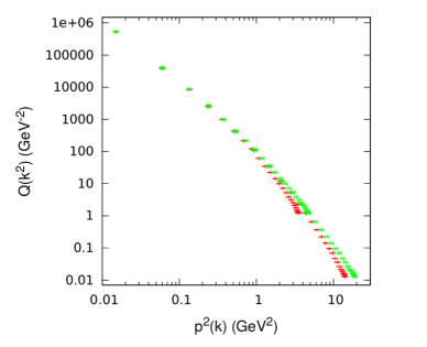
Figure 1: The Bose-ghost propagator $Q(k^{2})$, defined in Eq. (35), as a function of the unimproved (red, $+$) and of the improved (green, $\times$) momentum squared $p^{2}(k)$ [see Eqs. (39)–(41)]. We plot data for $\beta_{0}$ and $V=48^{4}$ using the sources defined in Eq. (30). Note the logarithmic scale on both axes.

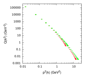
Figure 2: The Bose-ghost propagator $Q(k^{2})$, defined in Eq. (35), as a function of the unimproved (red, $+$) and of the improved (green, $\times$) momentum squared $p^{2}(k)$ [see Eqs. (39)–(41)]. We plot data for $\beta_{0}$ and $V=48^{4}$ using the sources defined in Eq. (32). Note the logarithmic scale on both axes.

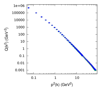
Figure 3: The Bose-ghost propagator $Q(k^{2})$, defined in Eq. (35), as a function of the improved momentum squared $p^{2}(k)$ [see Eqs. (40) and (41)] for the lattice volume $V=96^{4}$ at $\beta_{2}$. Here we plot data for the first (red, $+$), second (green, $\times$) and third (blue, $*$) proposed discretizations of the sources $B^{bc}_{\mu}(x)$ [see Eqs. (30)–(32) in Section III]. For the last case the data are multiplied by a factor 4. Note the logarithmic scale on both axes.

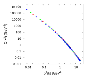
Figure 4: The Bose-ghost propagator $Q(k^{2})$, defined in Eq. (35), as a function of the improved momentum squared $p^{2}(k)$ [see Eqs. (40) and (41)]. We plot data for $\beta_{0}$ and $V=40^{4}$ (red, $+$), $48^{4}$ (green, $\times$), $64^{4}$ (blue, $*$), using the sources defined in Eq. (32). Note the logarithmic scale on both axes.

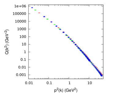
Figure 5: The Bose-ghost propagator $Q(k^{2})$, defined in Eq. (35), as a function of the improved momentum squared $p^{2}(k)$ [see Eqs. (40) and (41)]. We plot data for $\beta_{1}$ and $V=48^{4}$ (red, $+$), $60^{4}$ (green, $\times$), $72^{4}$ (blue, $*$), using the sources defined in Eq. (32). Note the logarithmic scale on both axes.

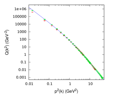
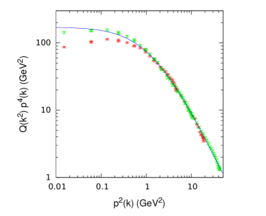
Figure 6: The Bose-ghost propagator $Q(k^{2})$ (top) [see Eq. (35)] and the rescaled Bose-ghost propagator $Q(k^{2})p^{4}(k)$ (bottom), as a function of the improved momentum squared $p^{2}(k)$ [see Eqs. (40) and (41)]. We plot data for $\beta_{0}$, $V=48^{4}$ (red, $+$) and $\beta_{1}$, $V=72^{4}$ (green, $\times$), after applying a matching procedure Leinweber:1998uu ; Cucchieri:2003di to the former set of data. Here we use the sources defined in Eq. (32). We also plot, for $V=72^{4}$, a fit using Eq. (42) and the parameters in Table 3, with $c=37(4)$. Note the logarithmic scale on both axes.

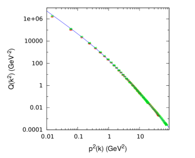
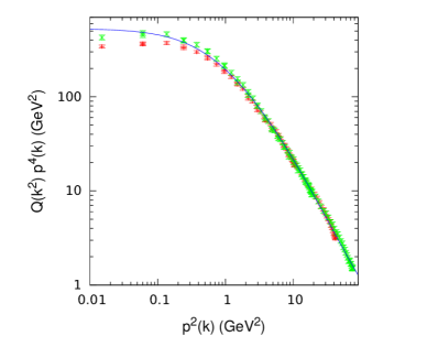
Figure 7: The Bose-ghost propagator $Q(k^{2})$ (top) [see Eq. (35)] and the rescaled Bose-ghost propagator $Q(k^{2})p^{4}(k)$ (bottom), as a function of the improved momentum squared $p^{2}(k)$ [see Eqs. (40) and (41)]. We plot data for $\beta_{1}$, $V=72^{4}$ (red, $\times$) and $\beta_{2}$, $V=96^{4}$ (green, $*$), after applying a matching procedure Leinweber:1998uu ; Cucchieri:2003di to the former set of data. Here we use the sources defined in Eq. (32). We also plot, for $V=96^{4}$, a fit using Eq. (42) and the parameters in Table 3, with $c=82(5)$. Note the logarithmic scale on both axes.

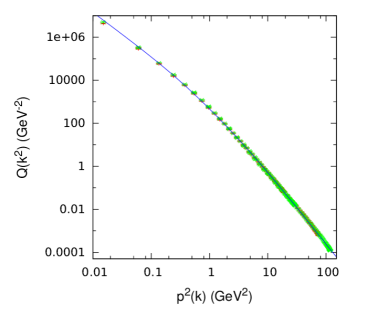
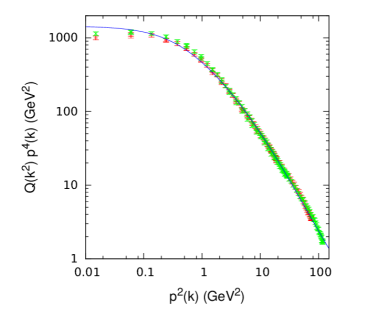
Figure 8: The Bose-ghost propagator $Q(k^{2})$ (top) [see Eq. (35)] and the rescaled Bose-ghost propagator $Q(k^{2})p^{4}(k)$ (bottom), as a function of the improved momentum squared $p^{2}(k)$ [see Eqs. (40) and (41)]. We plot data for $\beta_{2}$, $V=96^{4}$ (red, $\times$) and $\beta_{3}$, $V=120^{4}$ (green, $*$), after applying a matching procedure Leinweber:1998uu ; Cucchieri:2003di to the former set of data. Here we use the sources defined in Eq. (32). We also plot, for $V=120^{4}$, a fit using Eq. (42) and the parameters in Table 3, with $c=132(11)$. Note the logarithmic scale on both axes.

The inversion of the FP matrix ${\cal M}^{ab}(x,y)$ is performed using a conjugate-gradient method, accelerated by even/odd preconditioning. After indicating with

$$\widetilde{R}^{ac}_{\mu}(k)\,=\,\frac{1}{\sqrt{V}}\sum_{x}R^{ac}_{\mu}(x)\,e^{2\pi ik\cdot x/N}$$ (33)

the Fourier transform of the outcome $R^{ac}_{\mu}(x)$ of the numerical inversion [see Eq. (23)], it is clear that we can evaluate the Bose-ghost propagator [see Eq. (22)] in momentum space by considering

$$Q^{abcd}_{\mu\nu}(k)\,\equiv\,\Re\,\left\{\,\widetilde{R}^{ab}_{\mu}(k)\,\widetilde{R}^{cd}_{\nu}(-k)\,\right\}\;.$$ (34)

(In the above equations, $N$ is the lattice side, $k$ is the wave vector with components $k_{\mu}=0,1,\ldots,N-1$ and $\Re$ indicates the real part of the expression within brackets.) Then, by contracting the color indices $b,d$ and the Lorentz indices $\mu,\nu$, we can write [see Eq.16)]

$$Q^{ac}(k)\,\equiv\,Q^{abcb}_{\mu\mu}(k)\,\equiv\,\delta^{ac}\,P_{\mu\mu}(k)\,Q(k^{2})\;,$$ (35)

due to global color invariance. The numerical evaluation of the scalar function $Q(k^{2})$, through lattice Monte Carlo simulations, is the goal of this work.

The function $\widetilde{R}^{ac}_{\mu}(k)$ defined in Eq. (33) has been evaluated —for the three different choices for the lattice sources $B^{bc}_{\mu}(x)$ considered here— for all possible values of the color indices $a,c$ and of the Lorentz index $\mu$, and for two types of momenta, namely wave vectors whose components are $(0,0,0,k)$ and $(k,k,k,k)$, with $k=1,2,\ldots,N/2$. This gives $N$ different values for the momentum $p$. Note that the null momentum trivially gives $\widetilde{R}^{ac}_{\mu}(0)=0$. Indeed, if we indicate with $\psi^{b}_{n}(y)$ the eigenvectors of the FP matrix ${\cal M}^{ab}(x,y)$ and with $\lambda_{n}$ the corresponding eigenvalues, then we can write

$$({\cal M}^{-1})^{ab}(x,y)\,=\,\sum_{n\neq 0}\frac{\psi^{a}_{n}(x)\,\left[\psi^{b}_{n}(y)\right]^{*}}{\lambda_{n}}\;,$$ (36)

where ^∗ indicates complex conjugation and $\lambda_{0}=0$ is the trivial null eigenvalue, corresponding to constant eigenvectors. This implies

$$\widetilde{R}^{ac}_{\mu}(k) = \frac{1}{\sqrt{V}}\sum_{n\neq 0}\frac{1}{\lambda_{n}}\,\left(\left\{\sum_{z}\,B^{ec}_{\mu}(z)\,\left[\psi^{e}_{n}(z)\right]^{*}\right\}\right.$$ (37)

$$\qquad\;\;\left.\left[\sum_{x}\,\psi^{a}_{n}(x)\,e^{2\pi ik\cdot x/N}\right]\,\right)\;.$$

By recalling that eigenvectors corresponding to distinct eigenvalues of symmetric matrices are orthogonal, i.e. $\psi_{0}=constant$ is orthogonal to the eigenvectors $\psi^{a}_{n}(x)$ with $n\neq 0$, we have

$$\sum_{x}\,\psi^{a}_{n}(x)\,=\,0$$ (38)

for every $n\neq 0$ and therefore $\widetilde{R}^{ac}_{\mu}(k=0)=0$.

Our numerical code is parallelized using MPI and OpenMP. We always use four OpenMP threads for each MPI task and the 4-way Symmetrical Multiprocessing mode (SMP) for the runs on the Blue Gene/P supercomputer at Rice University. The total computing time was about 2.2 millions of CPU-hours. Further details on the implementation of the numerical simulations can be found in Ref. Cucchieri:2003zx .

IV Numerical Results

In this section we present the numerical results for the scalar function $Q(k^{2})$, defined in Eq. (35) above. In all cases the data points represent averages over gauge configurations and error bars correspond to one standard deviation (we consider the statistical error only). Also, in the plots, all quantities are in physical units. Let us stress that, compared to the results reported in Refs. Cucchieri:2014via ; Cucchieri:2014xfa , the data shown here have been divided by an additional factor 3.

We first investigate the effect of rotational-symmetry breaking on our results, by plotting the data for $Q(k^{2})$ as a function of two different definitions of the lattice momenta, i.e. the usual unimproved definition

$$p^{2}(k)\,=\,\sum_{\mu}p_{\mu}^{2}$$ (39)

and the improved definition Ma:1999kn

$$p^{2}(k)\,=\,\sum_{\mu}\left[\,p_{\mu}^{2}(k)+\frac{p_{\mu}^{4}(k)}{12}\,\right]\;,$$ (40)

where

$$p_{\mu}(k)\,=\,2\sin{\left(\frac{\pi k_{\mu}}{N}\right)}\;.$$ (41)

In Figs. 1 and 2 we show our data for $Q(k^{2})$ —respectively using the lattice definition of the sources $B^{bc}_{\mu}(x)$ given in Eqs. (30) and (32)— as a function of the unimproved and of the improved momentum squared $p^{2}(k)$. As one can see, the improved definition (40)–(41) makes the behavior of the propagator smoother at large momenta, allowing a better fit to the data. We also check (see Fig. 3) that our results do not depend on the choice of the lattice definition for the source (see discussion in the previous section). Finally, in Figs. 4 and 5, which refer respectively to the cases $\beta_{0}$ and $\beta_{1}$ at about the same physical volume, we consider the extrapolation to the infinite-volume limit. It is clear that the use of larger lattice volumes does not modify the behavior of the propagator, i.e. finite-size effects —at a given lattice momentum $p$— are essentially negligible. Thus, large volumes are relevant only to clarify the IR behavior of the Bose-ghost propagator.

In order to extrapolate our data to the continuum limit, we compare data obtained at different $\beta$ values, using the largest physical volumes available for comparison. In particular, in the top plot of Fig. 6 we show the data at $\beta_{0}$ with $V=48^{4}$ and at $\beta_{1}$ with $V=72^{4}$, which correspond to the same physical volume, after rescaling the data at $\beta_{0}$ using the matching technique described in Ref. Leinweber:1998uu ; Cucchieri:2003di . Similarly, in the top plot of Fig. 7 we compare the data for $\beta_{1}$ with $V=72^{4}$ and $\beta_{2}$ with $V=96^{4}$, and in the top plot of Fig. 8 we compare the data for $\beta_{2}$ with $V=96^{4}$ and $\beta_{3}$ with $V=120^{4}$, always applying a rescaling to the coarser set of data. The data clearly scale quite well, even though small deviations are observable in the IR limit [see the bottom plots in Figs. 6, 7 and 8, where we show the Bose-ghost propagator $Q(k^{2})$ multiplied by $p^{4}(k)$]. We thus observe discretization effects for the coarser lattices. Nevertheless, these effects decrease as the lattice spacing $a$ goes to zero. Indeed, the ratios between the finer and the coarser data —at the smallest momentum $p^{2}(k)\approx 0.015\,GeV^{2}$— in the various cases are, respectively, equal to 1.66(7), 1.25(9) and 1.14(9) in the plots shown in Figs. 6–8, with errors obtained from propagation of errors.

As done in Refs. Cucchieri:2014via ; Cucchieri:2014xfa , we also fit the data using the fitting function

$$f(p^{2})\,=\,\frac{c}{p^{4}}\,\frac{p^{2}+s}{p^{4}\,+\,u^{2}p^{2}\,+\,t^{2}}\;,$$ (42)

which is based on the analysis carried on in Refs. Zwanziger:2009je ; Zwanziger:2010iz , i.e. on the relation (obtained using a cluster decomposition)

$$Q(p^{2})\,\sim\,g_{0}^{2}\,G^{2}(p^{2})\,D(p^{2})\;,$$ (43)

where $D(p^{2})$ is the gluon propagator and $G(p^{2})$ is the ghost propagator. Then, one can view the above fitting function as generated by an IR-free FP ghost propagator $G(p^{2})\sim 1/p^{2}$ and by a massive gluon propagator $D(p^{2})$ Cucchieri:2007rg ; Cucchieri:2008fc ; Boucaud:2011ug . The fit describes the data quite well (see the $\chi^{2}/\mbox{d.o.f.}$ values in Table 3), even though in the IR limit there is a small discrepancy between the data and the fitting function considered (see bottom plots in Figs. 6–8).

Let us note that the fitted value for the parameter $c$ is somewhat arbitrary, since one can always fix a renormalization condition at a given scale $p^{2}=\mu^{2}$, which in turn yields a rescaling of the Bose-ghost propagator by a global factor. One should also note that, from Eqs. (22) and (23), it is clear that the propagator $Q(p^{2})$ evaluated in this work has a renormalization constant $Z_{Q}$ equal to one Zwanziger:2009je in the so-called Taylor scheme Boucaud:2008gn and in the algebraic renormalization scheme Vandersickel:2012tz . This implies that $Z_{Q}$ is also finite in any renormalization scheme (see e.g. Refs. Boucaud:2008gn ; Boucaud:2005ce for a discussion on this issue).

$V=N^{4}$	$\beta$	$t\,(GeV^{2})$	$u\,(GeV)$	$s\,(GeV^{2})$	$\chi^{2}/\mbox{d.o.f.}$
$\,48^{4}\,$	$\beta_{0}$	2.3(0.2)	1.5(0.2)	10.9(3.4)	6.57
$\,64^{4}\,$	$\beta_{0}$	2.2(0.2)	1.5(0.2)	8.7(2.4)	4.06
$\,72^{4}\,$	$\beta_{1}$	3.2(0.3)	3.6(0.4)	49(14)	2.45
$\,96^{4}\,$	$\beta_{2}$	3.0(0.1)	3.9(0.2)	57.8(9.5)	1.12
$\,120^{4}\,$	$\beta_{3}$	3.3(0.2)	4.8(0.3)	121(21)	1.98

Table 3: Parameters $t$, $u$ and $s$ from a fit of $f(p^{2})$ in Eq. (42) to the data. Errors in parentheses correspond to one standard deviation. The number of degrees of freedom (dof) is always $N-4$. We also show the reduced chi-squared $\chi^{2}/\mbox{dof}$. Fits have been done using gnuplot.

$V=N^{4}$	$\beta$	$v\,(GeV^{2})$	$w\,(GeV^{2})$	$b$ or $\alpha_{-}$	type
$\,48^{4}\,$	$\beta_{0}$	1.1(0.3)	2.0(0.2)	4.8(0.1)	1
$\,64^{4}\,$	$\beta_{0}$	1.1(0.3)	1.9(0.2)	4.0(0.1)	1
$\,72^{4}\,$	$\beta_{1}$	6.5(1.4)	5.6(0.2)	4.27(0.03)	-1
$\,96^{4}\,$	$\beta_{2}$	7.6(0.8)	6.99(0.04)	4.091(0.007)	-1
$\,120^{4}\,$	$\beta_{3}$	11.5(1.4)	11.04(0.06)	5.460(0.009)	-1

Table 4: Pole parameters [see Eqs. (44)–(49)] for the fitting function $f(p^{2})$, defined in Eq. (42). In the last column we report the type of poles obtained: the value 1 indicates complex-conjugate poles and the value -1 indicates real poles. Errors in parentheses have been obtained using a Monte Carlo error analysis (with 10000 samples).

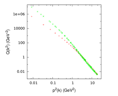
Figure 9: The Bose-ghost propagator $Q(k^{2})$ (red, $+$) —defined in Eq. (35)— and the product $g_{0}^{2}\,G^{2}(p^{2})\,D(p^{2})$ (green, $\times$) as a function of the improved momentum squared $p^{2}(k)$ [see Eqs. (40) e (41)] for the lattice volume $V=64^{4}$ at $\beta_{0}$. The data of the Bose-ghost propagator have been rescaled in order to agree with the data of the product $g_{0}^{2}\,G^{2}(p^{2})\,D(p^{2})$ at the largest momentum. Here we use the sources defined in Eq. (32). Note the logarithmic scale on both axes.

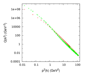
Figure 10: The Bose-ghost propagator $Q(k^{2})$ (red, $+$) —defined in Eq. (35)— and the product $g_{0}^{2}\,G^{2}(p^{2})\,D(p^{2})$ (green, $\times$) as a function of the improved momentum squared $p^{2}(k)$ [see Eqs. (40) e (41)] for the lattice volume $V=120^{4}$ at $\beta_{3}$. The data of the Bose-ghost propagator have been rescaled in order to agree with the data of the product $g_{0}^{2}\,G^{2}(p^{2})\,D(p^{2})$ at the largest momentum. Here we use the sources defined in Eq. (32). Note the logarithmic scale on both axes.

On the other hand, the parameters $t$, $u$ and $s$ can be related to the analytic structure of the Bose-ghost propagator $Q(p^{2})$. For example, one could rewrite the fitting function in terms of a pair of poles, i.e.

$$f(p^{2})\,=\,\frac{c}{p^{4}}\,\left(\frac{\alpha_{+}}{p^{2}+\omega_{+}^{2}}\,+\,\frac{\alpha_{-}}{p^{2}+\omega_{-}^{2}}\right)\;.$$ (44)

If the poles are complex-conjugate, i.e. if $\alpha_{\pm}=1/2\pm ib/2$ and $\omega_{\pm}^{2}=v\pm iw$, one has

$$f(p^{2})\,=\,\frac{c}{p^{4}}\,\frac{p^{2}\,+\,v+bw}{p^{4}\,+\,2v\,p^{2}\,+\,v^{2}+w^{2}}$$ (45)

and

$$s\,=\,v+bw\;,\qquad u^{2}\,=\,2v\;,\qquad t^{2}\,=\,v^{2}\,+\,w^{2}\;.$$ (46)

On the contrary, if the poles are real, i.e. if $\alpha_{\pm},\omega_{\pm}^{2}=v\pm w\in\mathbb{R}$, we have

$$f(p^{2})\,=\,\frac{c}{p^{4}}\,\frac{p^{2}\,+\,v+\left(\alpha_{-}-\alpha_{+}\right)w}{p^{4}\,+\,2v\,p^{2}\,+\,v^{2}-w^{2}}$$ (47)

and

$$\!\!\!\!\!\!\!s = v+\left(\alpha_{-}-\alpha_{+}\right)w\;,\qquad\quad\;u^{2}\,=\,2v\;,$$ (48)

$$\!\!\!\!\!\!\!t^{2} = v^{2}\,-\,w^{2}\;,\qquad\qquad\alpha_{+}+\alpha_{-}\,=\,1\;.$$ (49)

Results for these parametrizations for the poles are reported in Table 4 for the same lattice volumes considered in Table 3. (Errors, shown in parentheses, correspond to one standard deviation and were obtained using a Monte Carlo error analysis with 10000 samples). We find that, for the coarsest lattices, i.e. at $\beta_{0}=2.2$, these poles are complex-conjugate, with an imaginary part that is about twice the corresponding real part. This is in agreement with the results obtained for the gluon propagator in Ref. Cucchieri:2011ig at the same $\beta$ value. On the contrary, for the other three values of $\beta$ considered, we find that these poles are actually real, with $v\approx w$. In both cases, this fit supports the so-called massive solution of the coupled Yang-Mills Dyson-Schwinger equations of gluon and ghost propagators (see e.g. Refs. Aguilar:2004sw ; Aguilar:2006gr ; Aguilar:2008xm ; Binosi:2009qm ; Aguilar:2011ux ; Binosi:2012sj ) and the so-called Refined GZ approach Dudal:2008rm ; Dudal:2008sp ; Dudal:2011gd . For the cases $V=48^{4}$ and $64^{4}$ at $\beta_{0}$ we can compare our results in Table 3 with the analysis reported in Table II of Ref. Cucchieri:2011ig for the gluon propagator. One sees that the fitting parameters for the Bose-ghost propagator do not seem to relate in a simple way to the corresponding values obtained by fitting gluon-propagator data. There is indeed a visible discrepancy between the Bose-ghost propagator $Q(p^{2})$ and the product $g_{0}^{2}\,G^{2}(p^{2})\,D(p^{2})$, as one can see in Fig. 9 for the lattice volume $V=64^{4}$ at $\beta_{0}$. This discrepancy seems, however, to decrease at larger $\beta$ values (see Fig. 10).

Even though the simple Ansatz in Eq. (42) above gives a good description of the data, deviations can be seen in the IR region for momenta below about $1\,GeV$, by plotting the quantity $Q(k^{2})\,p^{4}(k)$ (see bottom plots in Figs. 6–8). We tried to improve our fits, by using more general forms of the Bose-ghost propagator. In particular, by considering the fitting forms for the gluon propagator used in Refs. Cucchieri:2003di ; Alkofer:2003jj we tried to include noninteger exponents in the fitting function $f(p^{2})$. Among the different possibilities considered, the best results have been obtained with the expression

$$f(p^{2})\,=\,\frac{c}{p^{4-2\eta}}\,\left(\frac{p^{2}+s}{p^{4}\,+\,u^{2}p^{2}\,+\,t^{2}}\right)^{1+\eta}\;,$$ (50)

which is a natural generalization of Eq. (42), while preserving the ultraviolet behavior $1/p^{6}$. Also, the above formula still allows a pole decomposition using Eqs. (46) and (49), respectively for the complex-conjugate poles and for the real poles. Results for these fits can be seen in Figs. 11–13, which should be compared to the corresponding fits in the bottom plots of Figs. 6–8. The fitting parameters are reported in Table 5. As one can see, by comparing Table 5 to Table 3, the value of $\chi^{2}/\mbox{d.o.f.}$ decreased visibly with the new fitting form, even though in some cases the fitting parameters are determined with very large errors (see, in particular, the results for the parameter $s$). Finally, also in this case we evaluated the parametrizations of the poles for the fitting curves (see Table 6). We find that, in all cases, the poles are real, with $v\approx w$.

Figure 11: The rescaled Bose-ghost propagator $Q(k^{2})p^{4}(k)$ [see Eq. (35)], as a function of the improved momentum squared $p^{2}(k)$ [see Eqs. (40) e (41)] for the data at $\beta_{1}$ and $V=72^{4}$. Here we use the sources defined in Eq. (32). We also plot a fit using Eq. (50) and the parameters in Table 5, with $c=15.5(9.1)$. Note the logarithmic scale on both axes.

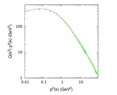
Figure 12: The rescaled Bose-ghost propagator $Q(k^{2})p^{4}(k)$ [see Eq. (35)], as a function of the improved momentum squared $p^{2}(k)$ [see Eqs. (40) e (41)] for the data at $\beta_{2}$ and $V=96^{4}$. Here we use the sources defined in Eq. (32). We also plot a fit using Eq. (50) and the parameters in Table 5, with $c=68.4(5.9)$. Note the logarithmic scale on both axes.

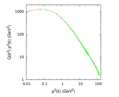
Figure 13: The rescaled Bose-ghost propagator $Q(k^{2})p^{4}(k)$ [see Eq. (35)], as a function of the improved momentum squared $p^{2}(k)$ [see Eqs. (40) e (41)] for the data at $\beta_{3}$ and $V=120^{4}$. Here we use the sources defined in Eq. (32). We also plot a fit using Eq. (50) and the parameters in Table 5, with $c=116(12)$. Note the logarithmic scale on both axes.

$V=N^{4}$	$\beta$	$t\,(GeV^{2})$	$u\,(GeV)$	$s\,(GeV^{2})$	$\eta$	$\chi^{2}/\mbox{d.o.f.}$
$\,48^{4}\,$	$\beta_{0}$	3.7(0.6)	4.2(0.8)	172(299)	0.19(2)	2.33
$\,64^{4}\,$	$\beta_{0}$	4.0(0.7)	4.3(0.9)	176(342)	0.16(2)	1.86
$\,72^{4}\,$	$\beta_{1}$	4.0(0.4)	6.0(0.8)	199(143)	0.19(3)	1.46
$\,96^{4}\,$	$\beta_{2}$	2.9(0.1)	5.2(0.3)	85(15)	0.24(4)	0.72
$\,120^{4}\,$	$\beta_{3}$	3.0(0.2)	6.0(0.4)	136(23)	0.30(7)	1.55

Table 5: Parameters $t$, $u$, $s$ and $\eta$ from a fit of $f(p^{2})$ in (50) to the data. Errors in parentheses correspond to one standard deviation. The number of degrees of freedom (dof) is always $N-5$. We also show the reduced chi-squared $\chi^{2}/\mbox{dof}$. Fits have been done using gnuplot.

$V=N^{4}$	$\beta$	$v\,(GeV^{2})$	$w\,(GeV^{2})$	$b$ or $\alpha_{+}$	type
$\,48^{4}\,$	$\beta_{0}$	8.8(3.4)	8.0(0.3)	10.69(0.04)	-1
$\,64^{4}\,$	$\beta_{0}$	9.2(3.9)	8.3(0.3)	10.50(0.04)	-1
$\,72^{4}\,$	$\beta_{1}$	18.0(4.8)	17.55(0.09)	5.66(0.01)	-1
$\,96^{4}\,$	$\beta_{2}$	13.5(1.6)	13.21(0.02)	3.206(0.004)	-1
$\,120^{4}\,$	$\beta_{3}$	18.0(2.4)	17.75(0.04)	3.824(0.006)	-1

Table 6: Pole parameters [see Eqs. (44)–(49)] for the fitting function $f(p^{2})$, defined in Eq. (50). In the last column we report the type of poles obtained: the value 1 indicates complex-conjugate poles and the value -1 indicates real poles. Errors in parentheses have been obtained using a Monte Carlo error analysis (with 10000 samples).

V Conclusions

As explained in the Introduction, breaking of the BRST symmetry in the GZ approach is linked to a nonzero value of the Gribov parameter $\gamma$, which is not assessed directly in lattice simulations. Nevertheless, this breaking may be also related to a nonzero value for the expectation value of a BRST-exact quantity such as the Bose-ghost propagator $Q^{abcd}_{\mu\nu}(x,y)$ defined in Eq. (8). The fact that this quantity can be evaluated on the lattice —in much the same way as the ghost propagator Suman:1995zg ; Cucchieri:1997dx — provides us with a suitable strategy to study the BRST-symmetry breaking of the GZ action numerically. These two manifestations of BRST-symmetry breaking are not independent, of course, since a nonzero value of $\gamma$ is necessary in both cases. Indeed, the fact that the lattice gauge-fixing is implemented by a minimization procedure is already equivalent to a nonzero value of $\gamma$, while the verification that the Bose-ghost propagator is itself nonzero provides nontrivial additional evidence for the breaking. Note that for $\gamma>1$ the breaking is more pronounced for the Bose-ghost propagator than for the action, the two being respectively of order $\gamma^{4}$ [see e.g. Eq. (16)] and $\gamma^{2}$ [see Eq. (15)].

In this work, we consider for the description of the Bose-ghost propagator the scalar function $Q(k^{2})$ defined in Eq. (35), obtained by contracting Lorentz and color indices in the original propagator. We recall that this propagator has been proposed as a carrier of the long-range confining force in minimal Landau gauge Zwanziger:2009je ; Furui:2009nj ; Zwanziger:2010iz . We have performed simulations for lattice volumes up to $120^{4}$ and for physical lattice extents up to $13.5$ fm, complementing previous results reported in Cucchieri:2014via ; Cucchieri:2014xfa . In particular, we present a more detailed discussion of the simulations and we investigate the approach to the infinite-volume and continuum limits. We find no significant finite-volume effects in the data. As for discretization effects, on the contrary, we observe small such effects for the coarser lattices, especially in the IR region. We also test different discretizations for the sources $B^{bc}_{\mu}(x)$ used in the inversion of the FP matrix and find that the data are fairly independent of the chosen lattice discretization of these sources.

Our results concerning the symmetry breaking and the form of the Bose-ghost propagator are similar to the previous analysis, i.e. we find a $1/p^{4}$ behavior in the IR regime and a $1/p^{6}$ behavior at large momenta. Also, when describing the data by polynomial fits, with the same fitting forms used in Cucchieri:2014via ; Cucchieri:2014xfa , we see that the description is relatively good, improving considerably for the finer lattices. In particular, plots of the rescaled propagator show much better agreement with the fit for the finer lattices. The same does not hold when using a modified fit with noninteger exponents as in Eq. (50). Indeed, in this case, although the values of $\chi^{2}/\mbox{d.o.f.}$ are generally better (but the fit has one extra parameter), the agreement does not get better as one moves to finer lattices.

Finally, in order to corroborate the results presented here and in Refs. Cucchieri:2014via ; Cucchieri:2014xfa , it would be, of course, important to evaluate numerically other correlation functions related to the breaking of the BRST symmetry in the GZ approach and, ultimately, obtain a lattice estimate of the Gribov parameter $\gamma$.

References

- (1) V. N. Gribov, Nucl. Phys. B 139, 1 (1978).
- (2) L. Giusti, M. L. Paciello, C. Parrinello, S. Petrarca and B. Taglienti, Int. J. Mod. Phys. A16, 3487 (2001).
- (3) D. Zwanziger, Nucl. Phys. B378, 525 (1992).
- (4) N. Vandersickel and D. Zwanziger, Phys. Rept. 520, 175 (2012).
- (5) D. Zwanziger, Phys. Rev. D81, 125027 (2010).
- (6) D. Zwanziger, arXiv:0904.2380 [hep-th].
- (7) N. Maggiore and M. Schaden, Phys. Rev. D50, 6616 (1994).
- (8) D. Zwanziger, Nucl. Phys. B412, 657 (1994).
- (9) L. von Smekal, M. Ghiotti and A. G. Williams, Phys. Rev. D78, 085016 (2008).
- (10) D. Dudal, J. A. Gracey, S. P. Sorella, N. Vandersickel and H. Verschelde, Phys. Rev. D78, 125012 (2008).
- (11) L. Baulieu and S. P. Sorella, Phys. Lett. B671, 481 (2009).
- (12) D. Dudal, S. P. Sorella, N. Vandersickel and H. Verschelde, Phys. Rev. D79, 121701 (2009).
- (13) S. P. Sorella, Phys. Rev. D80, 025013 (2009).
- (14) K. I. Kondo, arXiv:0905.1899 [hep-th].
- (15) S. P. Sorella et al., AIP Conf. Proc. 1361, 272 (2011).
- (16) M. A. L. Capri et al., Phys. Rev. D82, 105019 (2010).
- (17) D. Dudal and N. Vandersickel, Phys. Lett. B700, 369 (2011).
- (18) M. A. L. Capri et al., Phys. Rev. D83, 105001 (2011).
- (19) P. Lavrov, O. Lechtenfeld and A. Reshetnyak, JHEP 1110, 043 (2011).
- (20) A. Weber, Phys. Rev. D85, 125005 (2012).
- (21) P. M. Lavrov, O. V. Radchenko and A. A. Reshetnyak, Mod. Phys. Lett. A27, 1250067 (2012).
- (22) A. Weber, J. Phys. Conf. Ser. 378, 012042 (2012).
- (23) A. Maas, Mod. Phys. Lett. A27, 1250222 (2012).
- (24) D. Dudal and S. P. Sorella, Phys. Rev. D86, 045005 (2012).
- (25) M. A. L. Capri et al., Annals Phys. 339, 344 (2013).
- (26) V. Mader, M. Schaden, D. Zwanziger and R. Alkofer, Eur. Phys. J. C74, 2881 (2014).
- (27) A. Reshetnyak, Int. J. Mod. Phys. A29, 1450184 (2014).
- (28) N. Brambilla et al., Eur. Phys. J. C74, no. 10, 2981 (2014).
- (29) P. Y. Moshin and A. A. Reshetnyak, Nucl. Phys. B888, 92 (2014).
- (30) M. A. L. Capri, M. S. Guimaraes, I. F. Justo, L. F. Palhares and S. P. Sorella, Phys. Rev. D90, 085010 (2014).
- (31) M. Schaden and D. Zwanziger, Phys. Rev. D92, no. 2, 025001 (2015).
- (32) A. A. Reshetnyak, arXiv:1412.8428 [hep-th].
- (33) M. A. L. Capri et al., Phys. Rev. D92, no. 4, 045039 (2015).
- (34) M. A. L. Capri et al., Phys. Rev. D93, no. 6, 065019 (2016).
- (35) S. Furui, PoS LAT2009, 227 (2009).
- (36) A. Cucchieri, D. Dudal, T. Mendes and N. Vandersickel, Phys. Rev. D90, 051501 (2014).
- (37) A. Cucchieri, D. Dudal, T. Mendes and N. Vandersickel, PoS LATTICE2014, 347 (2014).
- (38) J. A. Gracey, JHEP 1002, 009 (2010).
- (39) L. Baulieu, Phys. Rept. 129, 1 (1985).
- (40) J. A. Gracey, Eur. Phys. J. C70, 451 (2010).
- (41) H. Suman and K. Schilling, Phys. Lett. B373, 314 (1996).
- (42) A. Cucchieri, Nucl. Phys. B508, 353 (1997).
- (43) A. Cucchieri, Nucl. Phys. B521, 365 (1998).
- (44) J. Fingberg, U. M. Heller and F. Karsch, Nucl. Phys. B392, 493 (1993).
- (45) J. C. R. Bloch, A. Cucchieri, K. Langfeld and T. Mendes, Nucl. Phys. B687, 76 (2004).
- (46) A. Cucchieri and T. Mendes, PoS LAT2007, 297 (2007).
- (47) A. Cucchieri, D. Dudal, T. Mendes and N. Vandersickel, Phys. Rev. D85, 094513 (2012).
- (48) M. Creutz, Phys. Rev. D21, 2308 (1980).
- (49) S. L. Adler, Nucl. Phys. Proc. Suppl. 9, 437 (1989).
- (50) http://luscher.web.cern.ch/luscher/ranlux/
- (51) A. Cucchieri and T. Mendes, Nucl. Phys. B471, 263 (1996).
- (52) A. Cucchieri and T. Mendes, Nucl. Phys. Proc. Suppl. 53, 811 (1997).
- (53) A. Cucchieri and T. Mendes, Comput. Phys. Commun. 154, 1 (2003).
- (54) A. Cucchieri, T. Mendes and A. Mihara, Phys. Rev. D72, 094505 (2005).
- (55) A. Cucchieri, T. Mendes, G. Travieso and A. R. Taurines, hep-lat/0308005, in the Proceedings of the 15th Symposium on Computer Architecture and High Performance Computing, edited by L. M. Sato et al. (IEEE Computer Society Press, Los Alamitos CA), 123 (2003).
- (56) J. P. Ma, Mod. Phys. Lett. A15, 229 (2000).
- (57) D. B. Leinweber et al. [UKQCD Collaboration], Phys. Rev. D60, 094507 (1999) [Erratum-ibid. D61, 079901 (2000)].
- (58) A. Cucchieri, T. Mendes and A. R. Taurines, Phys. Rev. D67, 091502 (2003).
- (59) A. Cucchieri and T. Mendes, Phys. Rev. Lett. 100, 241601 (2008).
- (60) A. Cucchieri and T. Mendes, Phys. Rev. D78, 094503 (2008).
- (61) P. Boucaud et al., Few Body Syst. 53, 387 (2012).
- (62) P. Boucaud et al., Phys. Rev. D79, 014508 (2009).
- (63) P. Boucaud et al., hep-ph/0507104.
- (64) A. C. Aguilar and A. A. Natale, JHEP 0408, 057 (2004).
- (65) A. C. Aguilar and J. Papavassiliou, JHEP 0612, 012 (2006).
- (66) A. C. Aguilar, D. Binosi and J. Papavassiliou, Phys. Rev. D78, 025010 (2008).
- (67) D. Binosi and J. Papavassiliou, Phys. Rept. 479, 1 (2009).
- (68) A. C. Aguilar, D. Binosi and J. Papavassiliou, Phys. Rev. D84, 085026 (2011).
- (69) D. Binosi, D. Ibanez and J. Papavassiliou, Phys. Rev. D86, 085033 (2012).
- (70) D. Dudal, J. A. Gracey, S. P. Sorella, N. Vandersickel and H. Verschelde, Phys. Rev. D78, 065047 (2008);
- (71) D. Dudal, S. P. Sorella and N. Vandersickel, Phys. Rev. D84, 065039 (2011).
- (72) R. Alkofer, W. Detmold, C. S. Fischer and P. Maris, Phys. Rev. D70, 014014 (2004).