Torsional rigidity for regions
with a Brownian boundary

Abstract

Let ${\mathbb{T}}^{m}$ be the $m$-dimensional unit torus, $m\in{\mathbb{N}}$. The torsional rigidity of an open set $\Omega\subset{\mathbb{T}}^{m}$ is the integral with respect to Lebesgue measure over all starting points $x\in\Omega$ of the expected lifetime in $\Omega$ of a Brownian motion starting at $x$. In this paper we consider $\Omega={\mathbb{T}}^{m}\backslash\beta[0,t]$, the complement of the path $\beta[0,t]$ of an independent Brownian motion up to time $t$. We compute the leading order asymptotic behaviour of the expectation of the torsional rigidity in the limit as $t\to\infty$. For $m=2$ the main contribution comes from the components in ${\mathbb{T}}^{2}\backslash\beta[0,t]$ whose inradius is comparable to the largest inradius, while for $m=3$ most of ${\mathbb{T}}^{3}\backslash\beta[0,t]$ contributes. A similar result holds for $m\geq 4$ after the Brownian path is replaced by a shrinking Wiener sausage $W_{r(t)}[0,t]$ of radius $r(t)=o(t^{-1/(m-2)})$, provided the shrinking is slow enough to ensure that the torsional rigidity tends to zero. Asymptotic properties of the capacity of $\beta[0,t]$ in ${\mathbb{R}}^{3}$ and $W_{1}[0,t]$ in ${\mathbb{R}}^{m}$, $m\geq 4$, play a central role throughout the paper. Our results contribute to a better understanding of the geometry of the complement of Brownian motion on ${\mathbb{T}}^{m}$, which has received a lot of attention in the literature in past years.

AMS 2000 subject classifications. 35J20, 60G50.
Key words and phrases. Torus, Laplacian, Brownian motion, torsional rigidity, inradius, capacity, spectrum, heat kernel.

Acknowledgment. The authors acknowledge support by The Leverhulme Trust through International Network Grant Laplacians, Random Walks, Bose Gas, Quantum Spin Systems. EB is supported by SNSF-grant 20-100536/1. FdH is supported by ERC Advanced Grant 267356-VARIS and NWO Gravitation Grant 024.002.003-NETWORKS. The authors thank Greg Lawler for helpful discussions about capacity of the Wiener sausage.

1 Background, main results and discussion

Section 1.1 provides our motivation for looking at torsional rigidity, and points to the relevant literature. Section 1.2 introduces our main object of interest, the torsional rigidity of the complement of Brownian motion on the unit torus. Section 1.3 states our main theorems. Section 1.4 places these theorems in their proper context and makes a link with the principal Dirichlet eigenvalue of the complement. Section 1.5 gives a brief sketch of the main ingredients of the proofs and provides an outline of the rest of the paper.

1.1 Background on torsional rigidity

Let $(M,g)$ be a geodesically complete, smooth $m$-dimensional Riemannian manifold without boundary, and let $\Delta$ be the Laplace-Beltrami operator acting in $L^{2}(M)$. We will in addition assume that $M$ is stochastically complete. That is, Brownian motion on $M$, denoted by $(\tilde{\beta}(s),s\geq 0;\tilde{\mathbb{P}}_{x},x\in M)$, with generator $\Delta$ exists for all positive time. The latter is guaranteed if for example the Ricci curvature on $M$ is bounded from below. See [16] for further details. For an open, bounded subset $\Omega\subset M$, and $x\in\Omega$ we define the first exit time of Brownian motion by

$$\tilde{\tau}_{\Omega}=\inf\{s\geq 0\colon\,\tilde{\beta}(s)\notin\Omega\}.$$ (1.1)

It is well known that

$$u_{\Omega}(x;t)=\tilde{\mathbb{P}}_{x}[\tilde{\tau}_{\Omega}>t]$$ (1.2)

is the unique solution of

$$\frac{\partial u}{\partial t}=\Delta u,\,u(\,\cdot\,;t)\in H_{0}^{1}(\Omega),\,t>0,$$

with initial condition $u(x;0)=1$. The requirement $u(\,\cdot\,;t)\in H_{0}^{1}(\Omega),\,t>0,$ represents the Dirichlet boundary condition. If we denote the expected lifetime of Brownian motion in $\Omega$ by

$$v_{\Omega}(x)=\tilde{\mathbb{E}}_{x}[\tilde{\tau}_{\Omega}],\qquad x\in\Omega,$$ (1.3)

where $\tilde{\mathbb{E}}_{x}$ denotes expectation with respect to $\tilde{\mathbb{P}}_{x}$, then

$$v_{\Omega}(x)=\int_{0}^{\infty}dt\,u_{\Omega}(x;t).$$ (1.4)

It is straightforward to verify that $v_{\Omega}$, the torsion function for $\Omega$, is the unique solution of

$$-\Delta v=1,\,v\in H_{0}^{1}(\Omega).$$ (1.5)

The torsional rigidity of $\Omega$ is the set function defined by

$${\mathcal{T}}(\Omega)=\int_{\Omega}dx\,v_{\Omega}(x).$$ (1.6)

The torsional rigidity of a cross section of a cylindrical beam found its origin in the computation of the angular change when a beam of a given length and a given modulus of rigidity is exposed to a twisting moment. See for example [28].

From a mathematical point of view both the torsion function $v_{\Omega}$ and the torsional rigidity ${\mathcal{T}}(\Omega)$ have been studied by analysts and probabilists. Below we just list a few key results. In analysis, the torsion function is an essential ingredient for the study of gamma-convergence of sequences of sets. See chapter 4 in [10]. Several isoperimetric inequalities have been obtained for the torsional rigidity when $M={\mathbb{R}}^{m}$. If $\Omega\subset{\mathbb{R}}^{m}$ has finite Lebesgue measure $|\Omega|$, and $\Omega^{*}$ is the ball with the same Lebesgue measure, centred at $0$, then ${\mathcal{T}}(\Omega)\leq{\mathcal{T}}(\Omega^{*})$. The following stability result for torsional rigidity was obtained in [9]:

$$\frac{{\mathcal{T}}(\Omega^{*})-{\mathcal{T}}(\Omega)}{{\mathcal{T}}(\Omega^{*})}\geq C_{m}{\mathcal{A}}(\Omega)^{3}.$$

Here, ${\mathcal{A}}(\Omega)$ is the Fraenkel asymmetry of $\Omega$, and $C_{m}$ is an $m$-dependent constant. The Kohler-Jobin isoperimetric inequality [17],[18] states that

$$\lambda_{1}(\Omega)^{(m+2)/2}\,{\mathcal{T}}(\Omega)\geq\lambda_{1}(\Omega^{*})^{(m+2)/2}\,{\mathcal{T}}(\Omega^{*}).$$

Stability results have also been obtained for the Kohler-Jobin inequality [9]. A classical isoperimetric inequality [27] states that

$$\|v_{\Omega}\|_{L^{\infty}(\Omega)}\leq v_{\Omega^{*}}(0).$$

In probability, the first exit time moments of Brownian motion have been studied in for example [4] and [20]. These moments are Riemannian invariants, and the $L^{1}$-norm of the first moment is the torsional rigidity.

The heat content of $\Omega$ at time $t$ is defined as

$$H_{\Omega}(t)=\int_{\Omega}u_{\Omega}(x;t)\,dx.$$ (1.7)

This quantity represents the amount of heat in $\Omega$ at time $t$, if $\Omega$ is at initial temperature $1$, while the boundary of $\Omega$ is at temperature $0$ for all $t>0$. By (1.2), $0\leq u_{\Omega}\leq 1$, and so

$$0\leq H_{\Omega}(t)\leq|\Omega|.$$

Finally by (1.4), (1.6) and (1.7) we have that

$${\mathcal{T}}(\Omega)=\int_{0}^{\infty}H_{\Omega}(t)\,dt,$$ (1.8)

i.e., the torsional rigidity is the integral of the heat content.

1.2 Torsional rigidity of the complement of Brownian motion

In the present paper we consider the flat unit torus ${\mathbb{T}}^{m}$. Let $(\beta(s),s\geq 0;{\mathbb{P}}_{x},x\in{\mathbb{T}}^{m})$ be a second independent Brownian motion on ${\mathbb{T}}^{m}$. Our object of interest is the random set (see Fig. 1)

$${\mathcal{B}}(t)={\mathbb{T}}^{m}\backslash\beta[0,t].$$

In particular, we are interested in the expected torsional rigidity of ${\mathcal{B}}(t)$:

$$\spadesuit(t)={\mathbb{E}}_{0}\big{(}{\mathcal{T}}\big{(}{\mathcal{B}}(t)\big{)}\big{)},\qquad t\geq 0.$$ (1.9)

Since $|{\mathbb{T}}^{m}|=1$ and $|\beta[0,t]|=0$, the torsional rigidity is the expected time needed by the first Brownian motion $\tilde{\beta}$ to hit $\beta[0,t]$ averaged over all starting points in ${\mathbb{T}}^{m}$. As $t\to\infty$, $\beta[0,t]$ tends to fill ${\mathbb{T}}^{m}$. Hence we expect that $\lim_{t\to\infty}\spadesuit(t)=0$. The results in this paper identify the speed of convergence. This speed provides information on the random geometry of ${\mathcal{B}}(t)$. In earlier work [6] we considered the inradius of ${\mathcal{B}}(t)$.

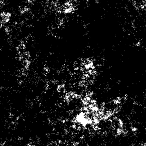
Figure 1: Simulation of $\beta[0,t]$ for $t=15$ and $m=2$. The Brownian path $\beta[0,t]$ is black, its complement ${\mathcal{B}}(t)={\mathbb{T}}^{m}\backslash\beta[0,t]$ is white.

The case $m=1$ is uninteresting. For $m=2$, as $t$ gets large the set ${\mathcal{B}}(t)$ decomposes into a large number of disjoint small components (see Fig. 1), while for $m\geq 3$ it remains connected. As shown in [14], in the latter case ${\mathcal{B}}(t)$ consists of “lakes” connected by “narrow channels”, so that we may think of it as a porous medium. Below we identify the asymptotic behaviour of $\spadesuit(t)$ as $t\to\infty$ when $m=2,3$.

For $m\geq 4$ we have $\spadesuit(t)=\infty$ for all $t\geq 0$ because Brownian motion is polar. To get a non-trivial scaling, the Brownian path must be thickened to a shrinking Wiener sausage

$$W_{r(t)}[0,t]=\big{\{}x\in{\mathbb{T}}^{m}\colon\,d_{t}(x)\leq r(t)\big{\}},\qquad t>0,$$ (1.10)

where $r\colon\,(0,\infty)\to(0,\infty)$ is such that $\lim_{t\to\infty}t^{1/(m-2)}r(t)=0$. This choice of shrinking is appropriate because for $m\geq 3$ typical regions in ${\mathcal{B}}(t)$ have a size of order $t^{-1/(m-2)}$ (see [11] and [14]). The object of interest is the random set

$${\mathcal{B}}_{r(t)}(t)={\mathbb{T}}^{m}\backslash W_{r(t)}[0,t],$$

in particular, the expected torsional rigidity of ${\mathcal{B}}_{r(t)}(t)$:

$$\spadesuit_{r(t)}(t)={\mathbb{E}}_{0}\big{(}{\mathcal{T}}\big{(}{\mathcal{B}}_{r(t)}(t)\big{)}\big{)},\qquad t>0.$$

Below we identify the asymptotic behaviour of $\spadesuit_{r(t)}(t)$ as $t\to\infty$ for $m\geq 4$ subject to a condition under which $r(t)$ does not decay too fast.

1.3 Asymptotic scaling of expected torsional rigidity

Theorems 1.1–1.3 below are our main results for the scaling of $\spadesuit(t)$ and $\spadesuit_{r(t)}(t)$ as $t\to\infty$. In what follows we write $f\asymp g$ when $0<c\leq f(t)/g(t)\leq C<\infty$ for $t$ large enough.

Theorem 1.1

If $m=2$, then

$$\spadesuit(t)\asymp t^{1/4}\,e^{-4(\pi t)^{1/2}},\qquad t\to\infty.$$ (1.11)

Theorem 1.2

If $m=3$, then

$$\spadesuit(t)=[1+o(1)]\,\frac{2}{t^{2}}\,{\mathbb{E}}_{0}\left(\frac{1}{\mathrm{cap}\,(\beta[0,1])^{2}}\right),\qquad t\to\infty,$$ (1.12)

where $\mathrm{cap}\,(\beta[0,1])$ is the Newtonian capacity of $\beta[0,1]$ in ${\mathbb{R}}^{3}$. All inverse moments of $\mathrm{cap}\,(\beta[0,1])$ are finite.

Theorem 1.3

If $m\geq 4$ and

$$\lim_{t\to\infty}t^{1/(m-2)}r(t)=0,\qquad\left\{\begin{array}[]{ll}m=4\colon&\lim\limits_{t\to\infty}\frac{t}{\log^{3}t}\,\frac{1}{\log(1/r(t))}=\infty,\\[5.69046pt] m\geq 5\colon&\lim\limits_{t\to\infty}\frac{t}{\log^{3}t}\,r(t)^{m-4}=\infty,\end{array}\right.$$ (1.13)

then

$$\spadesuit_{r(t)}(t)=[1+o(1)]\,\frac{1}{\kappa_{m}\,t^{2/(m-2)}}\,{\mathbb{E}}_{0}\left(\frac{1}{\mathrm{cap}\,(W_{\varepsilon(t)}[0,1])}\right),\qquad t\to\infty,$$ (1.14)

where $\varepsilon(t)=t^{1/(m-2)}r(t)$, $\mathrm{cap}\,(W_{\varepsilon}[0,1])$ is the Newtonian capacity of $W_{\varepsilon}[0,1]$ in ${\mathbb{R}}^{m}$, and where $\kappa_{m}$ is the Newtonian capacity of the ball with radius $1$ in ${\mathbb{R}}^{m}$,

$$\kappa_{m}=4\pi^{m/2}\Big{/}\,\Gamma\left(\frac{m-2}{2}\right).$$ (1.15)

All inverse moments of $\mathrm{cap}\,(W_{\varepsilon}[0,1])$ are finite for all $\varepsilon>0$.

We expect that similar results hold when ${\mathbb{T}}^{m}$ is replaced by a smooth $m$-dimensional compact connected Riemannian manifold without boundary. We further expect that the torsional rigidity satisfies a strong law of large numbers for $m\geq 3$ but not for $m=2$.

A key ingredient in the proof of Theorem 1.3 is the following scaling behaviour of the capacity of the Wiener sausage for $m\geq 4$. Let

$${\mathcal{C}}(t)=\left\{\begin{array}[]{ll}{\displaystyle\frac{\log t}{t}}\,\mathrm{cap}\,(W_{1}[0,t]),&m=4,\\[5.69046pt] {\displaystyle\frac{1}{t}}\,\mathrm{cap}\,(W_{1}[0,t]),&m\geq 5.\end{array}\right.$$ (1.16)

Then there exist constants $c_{m}\in(0,\infty)$, $m\geq 4$, such that

$${\mathcal{C}}(t)=[1+o(1)]\,c_{m}\quad\text{ in ${\mathbb{P}}_{0}$-probability as }t\to\infty.$$ (1.17)

In Section 7 we prove (1.17) for $m\geq 5$ with the help of subadditivity. For $m=4$, (1.17) is proven in [3].

1.4 Discussion

We refer the reader to [14] and [5] for an overview of what is known about the geometry of the complement of Brownian motion on the unit torus.

1. Theorems 1.1 and 1.2 identify the scaling of the expected torsional rigidity in low dimensions. This scaling may be viewed in the following context. Let $d(x,y)$ denote the distance between $x,y\in{\mathbb{T}}^{m}$. The distance of $x$ to $\beta[0,t]$ is denoted by

$$d_{t}(x)=\min_{y\in\beta[0,t]}d(x,y).$$ (1.18)

The inradius of ${\mathcal{B}}(t)$ is the random variable $\rho_{t}$ defined by

$$\rho_{t}=\max_{x\in{\mathbb{T}}^{m}}d_{t}(x).$$

A detailed analysis of $\rho_{t}$ and related quantities was given in [12], [5] for $m=2$ and in [11], [14] for $m\geq 3$. In [6] it was shown that for $m=2$,

$${\mathbb{E}}_{0}(\rho_{t})=e^{-(\pi t)^{1/2}[1+o(1)]},\qquad t\to\infty,$$ (1.19)

while for $m\geq 3$,

$${\mathbb{E}}_{0}(\rho_{t})=[1+o(1)]\,\left(\frac{m}{(m-2)\kappa_{m}}\,\frac{\log t}{t}\right)^{1/(m-2)},\qquad t\to\infty.$$ (1.20)

A ball of radius $r$ in ${\mathbb{T}}^{m}$ with $r$ sufficiently small has a torsional rigidity proportional to $r^{m+2}$. Theorem 1.1 and (1.19) show that $\log\spadesuit(t)=-[1+o(1)]\,4(\pi t)^{1/2}=[1+o(1)]\,\log{\mathbb{E}}_{0}(\rho_{t})^{4}$ for $m=2$, while Theorem 1.2 and (1.20) show that $\spadesuit(t)\asymp t^{-2}\gg{\mathbb{E}}_{0}(\rho_{t})^{5}$ for $m=3$. Thus, for $m=2$ the main contribution to the asymptotic behaviour of $\log\spadesuit(t)$ comes from the components in ${\mathcal{B}}(t)$ that have a size of order $\rho_{t}$ (which are atypical; see [12] and [5]), while for $m=3$ the main contribution to the asymptotic behaviour of $\spadesuit(t)$ comes from regions in ${\mathcal{B}}(t)$ that have a size of order $t^{-1}$ (which are typical; see [11] and [14]), i.e., most of ${\mathcal{B}}(t)$ contributes.

2. For $m=2$ it is shown in [5] that

$$\rho_{t}=t^{-1/8+o(1)}\,e^{-(\pi t)^{1/2}}\quad\text{in ${\mathbb{P}}_{0}$-probability},\qquad t\to\infty,$$ (1.21)

which is a considerable sharpening of (1.19). The proof is long and difficult. Combining (1.21) with what we found in Theorem 1.1, we get the relation

$$\spadesuit(t)\asymp t^{3/4+o(1)}\,{\mathbb{E}}_{0}(\rho_{t})^{4},$$ (1.22)

provided (1.21) also holds in mean (which is expected but has not been proved). Clearly, $\spadesuit(t)$ is not dominated by the largest component in ${\mathcal{B}}(t)$ alone: smaller components contribute too as long as they have a comparable size. The scaling in (1.22) suggests that the number of such components is of order $t^{3/4+o(1)}$. In order to settle this issue, we would need to strengthen Theorem 1.1 to tightness.

3. Theorem 1.3 identifies the scaling of the expected torsional rigidity in high dimensions. Via the scaling relation in distribution

$$\mathrm{cap}\,(W_{\varepsilon}[0,1])=\mathrm{cap}\,(\varepsilon W_{1}[0,\varepsilon^{-2}])=\varepsilon^{m-2}\mathrm{cap}\,(W_{1}[0,\varepsilon^{-2}]),\qquad\varepsilon>0,$$ (1.23)

it follows from (1.16)–(1.17) that $\mathrm{cap}\,(W_{\varepsilon}[0,1])=[1+o(1)]\,c_{m}\varepsilon^{m-4}$ in ${\mathbb{P}}_{0}$-probability as $\varepsilon\downarrow 0$ when $m\geq 5$. In that case Theorem 1.3 yields the asymptotics

$$\spadesuit_{r(t)}(t)=[1+o(1)]\,\frac{1}{\kappa_{m}c_{m}\,t\,r(t)^{m-4}},\qquad t\to\infty.$$ (1.24)

It also follows from (1.16)–(1.17) that $\mathrm{cap}\,(W_{\varepsilon}[0,1])=[1+o(1)]\,c_{4}/2\log(1/\varepsilon)$ in ${\mathbb{P}}_{0}$-probability as $\varepsilon\downarrow 0$ when $m=4$. In that case Theorem 1.3 yields the asymptotics

$$\spadesuit_{r(t)}(t)=[1+o(1)]\,\frac{2\log(1/t^{1/2}r(t))}{\kappa_{4}c_{4}\,t},\qquad t\to\infty.$$ (1.25)

By the second half of (1.13), both (1.24) and (1.25) correspond to the regime where $\spadesuit_{r(t)}(t)=o(1/\log^{3}t)$. We have not attempted to improve this to $o(1)$.

4. We did not investigate the regime for $m\geq 4$ where $r(t)$ decays so fast that $\spadesuit_{r(t)}(t)$ diverges as $t\to\infty$. In that regime, the Brownian motion $\tilde{\beta}$ in (1.1) runs around ${\mathbb{T}}^{m}$ many times before it hits $W_{r(t)}[0,t]$, and the growth of $\spadesuit_{r(t)}(t)$ depends on the global rather than the local properties of $W_{r(t)}[0,t]$.

5. We saw in Section 1.1 that the torsional rigidity is closely related to the principal Dirichlet eigenvalue. In Section 2 we will exhibit a relation with the square-integrated distance function and the largest inradius. In Section 6 we will give a quick proof of the following inequality relating the torsional rigidity to

$$\lambda_{1}\big{(}{\mathcal{B}}(t)\big{)},\quad\lambda_{1}\big{(}{\mathcal{B}}_{r(t)}(t)\big{)},$$ (1.26)

the principal Dirichlet eigenvalue of ${\mathcal{B}}(t)$ for $m=2,3$ and ${\mathcal{B}}_{r(t)}(t)$ for $m\geq 4$.

Theorem 1.4

(a) If $m=2,3$, then for $t$ large enough,

$${\mathbb{E}}_{0}\big{(}\lambda_{1}\big{(}{\mathcal{B}}(t)\big{)}\big{)}\geq\spadesuit(t)^{-2/(m+2)}.$$

(b) If $m\geq 4$ and $\lim_{t\to\infty}\spadesuit_{r(t)}(t)=0$, then for $t$ large enough,

$${\mathbb{E}}_{0}\big{(}\lambda_{1}\big{(}{\mathcal{B}}_{r(t)}(t)\big{)}\big{)}\geq\spadesuit_{r(t)}(t)^{-2/(m+2)}.$$

Combining the result for $m=2$ with what we found in Theorem 1.1, we obtain

$${\mathbb{E}}_{0}\big{(}\lambda_{1}\big{(}{\mathcal{B}}(t)\big{)}\big{)}\succeq t^{-1/8}\,e^{2(\pi t)^{1/2}},$$ (1.27)

where $f\succeq g$ means that $f(t)/g(t)\geq c>0$ for $t$ large enough. In [6] we conjectured that $\log{\mathbb{E}}_{0}(\lambda_{1}({\mathcal{B}}(t)))$ $=[1+o(1)]\,2(\pi t)^{1/2}$, which fits the lower bound in (1.27). However, a better estimate than (1.27) is possible. Namely, in Section 2 we will see that $\lambda_{1}({\mathcal{B}}(t))\asymp 1/\rho_{t}^{2}$, and so Jensen’s inequality gives the lower bound ${\mathbb{E}}_{0}(\lambda_{1}({\mathcal{B}}(t))\geq 1/{\mathbb{E}}_{0}(\rho_{t})^{2}$. Assuming that the scaling in (1.21) also holds in mean (which is expected but has not been proved), we get

$${\mathbb{E}}_{0}\big{(}\lambda_{1}\big{(}{\mathcal{B}}(t)\big{)}\big{)}\succeq t^{1/4+o(1)}\,e^{2(\pi t)^{1/2}},$$ (1.28)

which is better than (1.27) by a factor $t^{3/8+o(1)}$. Presumably (1.28) captures the correct scaling behaviour.

1.5 Brief sketch and outline

For $m=2$, ${\mathcal{B}}(t)$ consists of countably many connected component and the expected lifetime is sensitive to the starting point. We make use of the Hardy inequality to relate the time-integrated heat content to the space integral $\int_{{\mathbb{T}}^{2}}\mathrm{dist}(x,\beta[0,t])^{2}\,dx$. Because of the symmetry of ${\mathbb{T}}^{2}$, the problem boils down to studying the distribution of $\mathrm{dist}(x,\beta[0,t])^{2}$ with $x\in{\mathbb{T}}^{2}$ chosen uniformly at random. This can be done by using a domain perturbation formula for the Dirichlet Laplacian eigenvalues.

For $m\geq 3$, ${\mathcal{B}}(t)$ has only one connected component and the proof is probabilistic. The starting point is the representation

$$\spadesuit(t)=\int_{0}^{\infty}ds\,\,({\mathbb{P}}\otimes\tilde{\mathbb{P}})\big{(}\beta[0,t]\cap\tilde{\beta}[0,s]=\emptyset\big{)}.$$

It is easy to see that $\tilde{\beta}$ hits $\beta[0,t]$ within time $o((\log t)^{-1}$) with a very high probability. For $s\leq(\log t)^{-1}$, the above integrand is the probability that $\beta$ avoids the small set $\tilde{\beta}[0,s]$ for a long time $t$. We appeal to a recursive argument to evaluate this probability. Roughly speaking, in each unit of time $\beta$ hits $\tilde{\beta}[0,s]$ with probability $\approx\mathrm{cap}\,(\tilde{\beta}[0,s])$.

Outline. The remainder of this paper is organised as follows. In Section 2 we recall some analytical facts about the torsional rigidity. In Sections 3–5 we prove Theorems 1.1–1.3, respectively. The proof of Theorem 1.4 is given in Section 6, while the proof of the scaling in (1.16)–(1.17) for $m\geq 5$ is given in Section 7.

2 Analytical facts for the torsional rigidity

Let $M$ be an $m$-dimensional Riemannian manifold without boundary that is both geodesically and stochastically complete. In most of this paper we focus on the case where $M$ is the $m$-dimensional unit torus ${\mathbb{T}}^{m}$. However, the results mentioned below hold in greater generality. We derive certain a priori estimates on the torsional rigidity that will be needed later on.

For an open set $\Omega\subset M$ with boundary $\partial\Omega$, and with finite Lebesgue measure $|\Omega|$, we denote the Dirichlet heat kernel by $p_{\Omega}(x,y;t)$, $x,y\in\Omega$, $t>0$. Recall that the Dirichlet heat kernel is non-negative, monotone in $\Omega$, symmetric. Thus, we have that

$$0\leq p_{\Omega}(x,y;t)\leq p_{M}(x,y;t).$$

Since $|\Omega|<\infty$, there exists an $L^{2}(\Omega)$ eigenfunction expansion for the Dirichlet heat kernel in terms of the Dirichlet eigenvalues $\lambda_{1}(\Omega)\leq\lambda_{2}(\Omega)\leq\cdots$, and a corresponding orthonormal set of eigenfunctions $\varphi_{1},\varphi_{2},\cdots$ in $L^{2}(\Omega)$:

$$p_{\Omega}(x,y;t)=\sum_{j\in{\mathbb{N}}}e^{-t\lambda_{j}(\Omega)}\varphi_{j}(x)\varphi_{j}(y).$$ (2.1)

Since

$$u_{\Omega}(x;t)=\int_{\Omega}p_{\Omega}(x,y;t)\,dy,$$

we have that

$$v_{\Omega}(x)=\int_{\Omega}dy\int_{0}^{\infty}dt\,\,p_{\Omega}(x,y;t),$$

and

$${\mathcal{T}}(\Omega)=\int_{0}^{\infty}dt\,\int_{\Omega}dx\,\int_{\Omega}dy\,p_{\Omega}(x,y;t).$$ (2.2)

Lemma 2.1 below provides an upper bound on the Dirichlet eigenfunctions in terms of the Dirichlet eigenvalues. This bound will show that the eigenfunctions are in $L^{\infty}({\mathbb{T}}^{m})$, which by Hölder’s inequality implies that they are in $L^{p}({\mathbb{T}}^{m})$ for all $1\leq p\leq\infty$. Lemma 2.2 below states upper and lower bounds on the torsional rigidity that will be needed later on.

Lemma 2.1

Suppose that $\Omega\subset M$, $|\Omega|<\infty$, $\sup_{x\in M}p(x,x;t)<\infty$ for all $t>0$. Then

$$\left\|\varphi_{j}\right\|_{L^{\infty}(\Omega)}^{2}\leq e\sup_{x\in M}p_{M}(x,x;\lambda_{j}(\Omega)^{-1}),\qquad j\in{\mathbb{N}}.$$ (2.3)

Proof.   By (2.1) and the domain monotonicity of the Dirichlet heat kernel ([16]), we have that

$$\varphi_{j}(x)^{2}\leq e\,p_{\Omega}(x,x;\lambda_{j}(\Omega)^{-1})\leq e\,p_{M}(x,x;\lambda_{j}(\Omega)^{-1}).$$ (2.4)

Taking first the supremum over $x\in M$ in the right-hand side of (2.4) and subsequently in the left-hand side of (2.4), we get (2.3).  

Let

$$\delta_{\Omega}(x)=\min_{y\in{\mathbb{R}}^{m}\backslash\Omega}d(x,y)$$ (2.5)

denote the distance of $x\in\Omega$ to ${\mathbb{R}}^{m}\backslash\Omega$.

Lemma 2.2

(a) Let $M$ be a Riemannian manifold that is both geodesically and stochastically complete. Let $\Omega$ be an open subset of $M$ with $|\Omega|<\infty$. Then

$${\mathcal{T}}(\Omega)\leq\lambda_{1}(\Omega)^{-1}|\Omega|.$$ (2.6)

(b) Suppose that $M$ and $\Omega$ satisfy the hypotheses in (a). Then

$${\mathcal{T}}(\Omega)\geq\lambda_{1}(\Omega)^{-1}\lVert\varphi_{1}\rVert_{L^{\infty}(\Omega)}^{-2}.$$ (2.7)

(c) Let $\Omega\subset{\mathbb{R}}^{m}$. Then

$${\mathcal{T}}(\Omega)\geq\frac{1}{2m}\int_{\Omega}\delta_{\Omega}(x)^{2}\,dx.$$ (2.8)

(d) Let $\Omega\subset{\mathbb{R}}^{2}$ be simply connected and $\delta_{\Omega}\in L^{2}(\Omega)$. Then

$${\mathcal{T}}(\Omega)\leq 16\int_{\Omega}\delta_{\Omega}(x)^{2}\,dx.$$ (2.9)

(e) Let $\Omega\subset{\mathbb{T}}^{m}$. Then $\Omega$ can be embedded in ${\mathbb{R}}^{m}$ if and only if $\max_{i=1}^{m}|x_{i}-y_{i}|\leq\frac{1}{2}$ for all $x=(x_{1},\ldots,x_{m})\in\Omega$ and $y=(y_{1},\ldots,y_{m})\in\Omega$. If $\Omega\subset{\mathbb{T}}^{2}$ can be embedded in ${\mathbb{R}}^{2}$, then

$$\frac{1}{4}\int_{\Omega}\delta_{\Omega}(x)^{2}\,dx\leq{\mathcal{T}}(\Omega)\leq 16\int_{\Omega}\delta_{\Omega}(x)^{2}\,dx.$$ (2.10)

Proof.   (a) Since the eigenfunctions are in all $L^{p}(\Omega)$, we have by (2.1), (2.2) and Parseval’s identity that

$${\mathcal{T}}(\Omega)=\int_{0}^{\infty}dt\,\sum_{j\in{\mathbb{N}}}e^{-t\lambda_{j}(\Omega)}\left(\int_{\Omega}\varphi_{j}\right)^{2}\leq\lambda_{1}(\Omega)^{-1}\sum_{j\in{\mathbb{N}}}\left(\int_{\Omega}\varphi_{j}\right)^{2}=\lambda_{1}(\Omega)^{-1}|\Omega|.$$ (2.11)

Inequality (2.6) goes back to [22]. For a recent discussion and further improvements we refer the reader to [8].
(b) By (1.8) andthe first identity in (2.11), we have that

$${\mathcal{T}}(\Omega)\geq\int_{0}^{\infty}e^{-t\lambda_{1}(\Omega)}\,dt\left(\int_{\Omega}\varphi_{1}\right)^{2}=\lambda_{1}(\Omega)^{-1}\left(\int_{\Omega}\varphi_{1}\right)^{2}.$$ (2.12)

By Lemma 2.1, we have that $\lVert\varphi_{1}\rVert_{L^{\infty}(\Omega)}<\infty$, and so

$$1=\int_{\Omega}\varphi_{1}^{2}\leq\lVert\varphi_{1}\rVert_{L^{\infty}(\Omega)}\int_{\Omega}|\varphi_{1}|.$$ (2.13)

Inequality (2.7) follows from (2.12),(2.13), and the fact that $\varphi_{1}$ does not change sign.
(c) For every $x\in\Omega$ the open ball $B_{\delta_{\Omega}(x)}(x)$ with centre $x$ and radius $\delta_{\Omega}(x)$ is contained in $\Omega$. Therefore, by domain monotonicity, the expected life time satisfies $v_{\Omega}(y)\geq v_{B_{\delta(x)}(x)}(y)$. Hence

$$v_{\Omega}(y)\geq v_{B_{\delta_{\Omega}(x)}(x)}(y)=\frac{\delta_{\Omega}(x)^{2}-|x-y|^{2}}{2m},\qquad|y-x|\leq\delta_{\Omega}(x).$$

Choose $y=x$, integrate over $x\in\Omega$ and use (1.6), to get the claim.
(d) It was shown in [2] that the Dirichlet Laplacian on a simply connected proper subset of ${\mathbb{R}}^{2}$ satisfies a strong Hardy inequality:

$$\int_{\Omega}|\nabla w(x)|^{2}\,dx\geq\frac{1}{16}\int_{\Omega}\frac{w(x)^{2}}{\delta_{\Omega}(x)^{2}}\,dx\qquad\forall\,w\in C_{c}^{\infty}(\Omega).$$

Theorem 1.5 in [7] implies (2.9).
(e) Recall that the metric on ${\mathbb{T}}^{m}$ is given by

$$d(x,y)=\left(\sum_{i=1}^{m}\min\big{\{}|x_{i}-y_{i}|,1-|x_{i}-y_{i}|\big{\}}^{2}\right)^{1/2}.$$

Note that $\textup{diam}({\mathbb{T}}^{m})=\tfrac{1}{2}\sqrt{m}$ because $\min\{|x_{i}-y_{i}|,1-|x_{i}-y_{i}|\}\leq\tfrac{1}{2}$. If $|x_{i}-y_{i}|\leq\tfrac{1}{2}$ for all $i$, then $d(x,y)=|x-y|$. Next, suppose that $d(x,y)=|x-y|$. Then $\sum_{i=1}^{m}\min\{|x_{i}-y_{i}|,1-|x_{i}-y_{i}|\}^{2}=\sum_{i=1}^{m}|x_{i}-y_{i}|^{2}$. Let $I=\{i\colon\,|x_{i}-y_{i}|>\tfrac{1}{2}\}$. Then $\sum_{i\in I}(1-2|x_{i}-y_{i}|)=0$. We therefore conclude that $I=\emptyset$. Finally, (2.10) follows from (2.8) for $m=2$ and (2.9).  

3 Torsional rigidity for $m=2$

In Section 3.1 we show that the inverse of the principal Dirichlet eigenvalue of ${\mathcal{B}}(1)={\mathbb{T}}^{2}\backslash\beta[0,1]$ has a finite exponential moment. In Section 3.2 we use this result to prove Theorem 1.1.

3.1 Exponential moment of the inverse principal Dirichlet eigenvalue

Lemma 3.1

There exists $c>0$ such that

$${\mathbb{E}}_{0}\left(\exp\left[\frac{c}{\lambda_{1}({\mathcal{B}}(1))}\right]\right)<\infty.$$

Proof.   Let $\mathrm{cap}\,(A)$ denote the logarithmic capacity of a measurable set $A\subset{\mathbb{R}}^{2}$. It is well known (see [19]) that if $\mathrm{cap}\,(A)>0$ and $\epsilon A$ is a homothety of $A$ by a factor $\epsilon$, then

$$\mathrm{cap}\,(\epsilon A)=\frac{2\pi}{\log(1/\varepsilon)}\,[1+o(1)],\qquad\varepsilon\downarrow 0,$$

and

$$\lambda_{1}({\mathbb{T}}^{2}\backslash\epsilon A)=\frac{2\pi}{\log(1/\varepsilon)}\,[1+o(1)],\qquad\varepsilon\downarrow 0.$$

In particular, if $L_{\varepsilon}$ is a straight line segment of length $\varepsilon$, then there exists a $c^{\prime}\in(0,\infty)$ such that

$$\lambda_{1}({\mathbb{T}}^{2}\backslash L_{\varepsilon})\geq\frac{c^{\prime}}{\log(1/\varepsilon)},\qquad 0<\varepsilon\leq\tfrac{1}{2}.$$

Since $\mathrm{cap}\,(\beta[0,1])\geq\mathrm{cap}\,(L_{|\beta(1)|})\geq\mathrm{cap}\,(L_{(\tfrac{1}{2}\wedge|\beta(1)|)})$, we get

$${\mathbb{E}}_{0} \left(\exp\left[\frac{c}{\lambda_{1}({\mathcal{B}}(1))}\right]\right)\leq{\mathbb{E}}_{0}\left((\tfrac{1}{2}\wedge|\beta(1)|)^{-c/c^{\prime}}\right)\leq(\tfrac{1}{2})^{-c/c^{\prime}}+{\mathbb{E}}_{0}\left(|\beta(1)|^{-c/c^{\prime}}\right)$$

$$=(\tfrac{1}{2})^{-c/c^{\prime}}+\int_{{\mathbb{R}}^{2}}|x|^{-c/c^{\prime}}\,\frac{1}{4\pi}\,e^{-|x|^{2}/4}\,dx,$$

which is finite when $c/c^{\prime}<2$.  

3.2 Proof of Theorem 1.1

Proof.   The proof comes in 6 Steps, and is based on Lemmas 3.2–3.5 below. We use the following abbreviations (recall (1.18) and (1.26)):

$$D^{2}_{t}=\int_{{\mathbb{T}}^{2}}d_{t}(x)^{2}\,dx,\qquad\lambda_{t}=\lambda_{1}({\mathcal{B}}(t)).$$ (3.1)

1. Note that $\beta[0,t]$ is a closed subset of ${\mathbb{T}}^{2}$ a.s. Hence ${\mathcal{B}}(t)$ is open and its components are open and countable. Let $\{\Omega_{1}(t),\Omega_{2}(t),\cdots\}$ enumerate these components. Let

$$\phi_{i}(t)=\mathrm{diam}(\Omega_{i}(t))=\sup_{x,y\in\Omega_{i}(t)}d(x,y),$$

and abbreviate

$${\mathcal{I}}_{u}(t)=\{i\in{\mathbb{N}}\colon\,\phi_{i}(t)\leq u\},\quad{\mathcal{E}}_{u}(t)=\left\{\sup_{i\in{\mathbb{N}}}\phi_{i}(t)>u\right\},\qquad u\in(0,1).$$

It follows from the proof of Lemma 2.2(d) that if $i\in{\mathcal{I}}_{1/2}(t)$, then $\Omega_{i}(t)$ can be isometrically embedded in ${\mathbb{R}}^{2}$. Since $\beta[0,t]$ is continuous a.s., each $\Omega_{i}(t)$ is simply connected. Since the torsional rigidity is additive on disjoint sets we have that

$${\mathcal{T}}({\mathcal{B}}(t))=\sum_{i\in{\mathbb{N}}}{\mathcal{T}}(\Omega_{i}(t))=\sum_{i\in{\mathcal{I}}_{1/2}(t)}{\mathcal{T}}(\Omega_{i}(t))+\sum_{i\notin{\mathcal{I}}_{1/2}(t)}{\mathcal{T}}(\Omega_{i}(t)).$$ (3.2)

2. The first term in the right-hand side of (3.2) is estimated from above by Lemma 2.2(d). This gives (recall (2.5))

$$\sum_{i\in{\mathcal{I}}_{1/2}(t)}{\mathcal{T}}(\Omega_{i}(t))\leq 16\sum_{i\in{\mathcal{I}}_{1/2}(t)}\int_{\Omega_{i}(t)}\delta_{\Omega_{i}(t)}(x)^{2}\,dx\leq 16\sum_{i\in{\mathbb{N}}}\int_{\Omega_{i}(t)}\delta_{\Omega_{i}(t)}(x)^{2}\,dx=16D^{2}_{t}.$$

The second term in the right-hand side of (3.2) is estimated from above by Lemma 2.2(a). This gives

$$\sum_{i\notin{\mathcal{I}}_{1/2}(t)}{\mathcal{T}}(\Omega_{i}(t))\leq\sum_{i\notin{\mathcal{I}}_{1/2}(t)}\lambda_{t}^{-1}\,|\Omega_{i}(t)|\leq 1_{{\mathcal{E}}_{1/2}(t)}\,\lambda_{t}^{-1}\sum_{i\in{\mathbb{N}}}|\Omega_{i}(t)|=1_{{\mathcal{E}}_{1/2}(t)}\,\lambda_{t}^{-1}.$$

By Cauchy-Schwarz, this term contributes to $\spadesuit(t)$ at most

$${\mathbb{E}}_{0}\left(1_{{\mathcal{E}}_{1/2}(t)}\,\lambda_{t}^{-1}\right)\leq\left({\mathbb{P}}_{0}({\mathcal{E}}_{1/2}(t))\right)^{1/2}\Big{(}{\mathbb{E}}_{0}\big{(}\lambda_{t}^{-2}\big{)}\Big{)}^{1/2}.$$ (3.3)

To bound the probability in the right-hand side of (3.3) from above, we let $\{Q_{1},\dots,Q_{N}\}$, $N=10^{4}$, be any open disjoint collection of squares in ${\mathbb{T}}^{2},$ each with area $10^{-4}$ and not containing $0$. Furthermore, we let $\bar{Q}_{N,\epsilon}$ be the open $\epsilon$-neighbourhood of the union of the boundaries of these squares with $\epsilon=10^{-3}$. Then $\beta[0,1]$ starting at $0$ has a positive probability $p^{\prime}=p^{\prime}(N,\epsilon)$ of making a closed loop around each of these squares and staying inside $\bar{Q}_{N,\epsilon}$. Translating $\{Q_{1},\dots,Q_{N}\}$ such that these squares do not contain $\beta(1)$, we find that $\beta[1,2]$ starting at $\beta(1)$ has a positive probability $p^{\prime}$ of making a closed loop around each of these translated squares and staying inside $\bar{Q}_{N,\epsilon}+\beta(1)$. Continuing this way, by induction we find that the probability of $\beta[0,t]$ not making any of these closed translated loops is at most $(1-p^{\prime})^{\lfloor t\rfloor}$, where $\lfloor\cdot\rfloor$ denotes the integer part. Hence ${\mathbb{P}}_{0}(\sup_{i\in{\mathbb{N}}}\phi_{i}(t)>\tfrac{1}{2})\leq(1-p^{\prime})^{\lfloor t\rfloor}$, and so

$${\mathbb{P}}_{0}({\mathcal{E}}_{1/2}(t))\leq e^{-pt},\qquad t\geq 2,$$ (3.4)

for some $p>0$. We conclude that

$$\spadesuit(t)\leq 16\,{\mathbb{E}}_{0}\left(D^{2}_{t}\right)+e^{-pt/2}\Big{(}{\mathbb{E}}_{0}(\lambda_{t}^{-2})\Big{)}^{1/2},\qquad t\geq 2.$$ (3.5)

Since $t\mapsto\lambda_{t}$ is non-decreasing, Lemma 3.1 implies that the second term decays exponentially fast in $t,$ and therefore is harmless for the upper bound in (1.11).

3. To derive a lower bound for $\spadesuit(t)$, we note that by Lemma 2.2(e) we have

$${\mathcal{T}}({\mathcal{B}}(t))=\sum_{i\in{\mathbb{N}}}{\mathcal{T}}(\Omega_{i}(t))\geq\sum_{i\in{\mathcal{I}}_{1/2}(t)}{\mathcal{T}}(\Omega_{i}(t))$$

$$\geq\tfrac{1}{4}\sum_{i\in{\mathcal{I}}_{1/2}(t)}\int_{\Omega_{i}(t)}\delta_{\Omega_{i}(t)}(x)^{2}\,dx\geq\tfrac{1}{4}\sum_{i\in{\mathbb{N}}}\int_{\Omega_{i}(t)}\delta_{\Omega_{i}(t)}(x)^{2}\,dx-\tfrac{1}{4}\sum_{i\notin{\mathcal{I}}_{1/2}(t)}\int_{\Omega_{i}(t)}\delta_{\Omega_{i}(t)}(x)^{2}\,dx$$

$$\geq\tfrac{1}{4}D^{2}_{t}-\tfrac{1}{4}\sum_{i\notin{\mathcal{I}}_{1/2}(t)}1_{{\mathcal{E}}_{1/2}(t)}\int_{\Omega_{i}(t)}\delta_{\Omega_{i}(t)}(x)^{2}\,dx\geq\tfrac{1}{4}D^{2}_{t}-\tfrac{1}{8}1_{{\mathcal{E}}_{1/2}(t)},$$

where in the last inequality we use that $\delta_{\Omega_{i}(t)}(x)\leq\textup{diam}({\mathbb{T}}^{2})=\tfrac{1}{2}\sqrt{2}$ and $|{\mathbb{T}}^{2}|=1$. We conclude by (3.4) that

$$\spadesuit(t)\geq\tfrac{1}{4}{\mathbb{E}}_{0}\left(D^{2}_{t}\right)-e^{-pt},\qquad t\geq 2.$$ (3.6)

The second term is again harmless for the lower bound in (1.11).

4. The estimates in (3.5) and (3.6) show that $\spadesuit(t)\asymp{\mathbb{E}}_{0}(D^{2}_{t})$ up to exponentially small error terms. In order to obtain the leading order asymptotic behaviour of ${\mathbb{E}}_{0}(D^{2}_{t})$, we make a dyadic partition of ${\mathbb{T}}^{2}$ into squares as follows. Partition ${\mathbb{T}}^{2}$ into four $1$-squares of area $\tfrac{1}{4}$ each. Proceed by induction to partition each $k$-square into four $(k+1)$-squares, etc. In this way, for each $k\in{\mathbb{N}}$, ${\mathbb{T}}^{2}$ is partitioned into $2^{2k}$ $k$-squares. We define a $k$-square to be good when the path $\beta[0,t]$ does not hit this square, but does hit the unique $(k-1)$-square to which it belongs. Clearly, if $x$ belongs to a good $k$-square, then $\textup{dist}(x,\beta[0,t])\leq(2\sqrt{2})2^{-k}$. Hence, as the area of each $k$-square is $2^{-2k}$, we get

$${\mathbb{E}}\left(D^{2}_{t}\right)\leq 8\sum_{k\in{\mathbb{N}}}2^{-2k}\sum_{S\textup{ is a k-square}}2^{-2k}\,{\mathbb{P}}(S\textup{ is a good square})\leq 8\sum_{k\in{\mathbb{N}}}2^{-4k}\,{\mathbb{E}}\left(\#\textup{ good }k\textup{-squares}\right),$$ (3.7)

where we write ${\mathbb{E}}=\int_{{\mathbb{T}}^{2}}dx\,{\mathbb{E}}_{x}$, which is the same as ${\mathbb{E}}_{0}$ for the quantity under consideration, by translation invariance. To estimate the right-hand side of (3.7) we need three lemmas.

Lemma 3.2

For $k\in{\mathbb{N}}$, let $p_{k}(t)={\mathbb{P}}(\beta[0,t]\cap S_{k})=\emptyset)$, where $S_{k}$ is any of the $k$-squares. Then

$$p_{k}(t)\leq e^{-t\lambda_{1}({\mathbb{T}}^{2}\backslash S_{k})}.$$

Proof.   Let $p_{{\mathbb{T}}^{2}\backslash S_{k}}(x,y;t)$ be the Dirichlet heat kernel for ${\mathbb{T}}^{2}\backslash S_{k}$. By the eigenfunction expansion in (2.1), we have that

$$p_{k}(t)=\int_{{\mathbb{T}}^{2}\backslash S_{k}}dx\int_{{\mathbb{T}}^{2}\backslash S_{k}}dy\,\,p_{{\mathbb{T}}^{2}\backslash S_{k}}(x,y;t)=\int_{{\mathbb{T}}^{2}\backslash S_{k}}dx\int_{{\mathbb{T}}^{2}\backslash S_{k}}dy\,\,\sum_{j\in{\mathbb{N}}}e^{-t\lambda_{j}({\mathbb{T}}^{2}\backslash S_{k})}\varphi_{j}(x)\varphi_{j}(y)$$

$$\leq e^{-t\lambda_{1}({\mathbb{T}}^{2}\backslash S_{k})}\sum_{j\in{\mathbb{N}}}\left(\int_{{\mathbb{T}}^{2}\backslash S_{k}}dx\,\varphi_{j}(x)\right)^{2}=e^{-t\lambda_{1}({\mathbb{T}}^{2}\backslash S_{k})}|{\mathbb{T}}^{2}\backslash S_{k}|\leq e^{-t\lambda_{1}({\mathbb{T}}^{2}\backslash S_{k})},$$

where we use Parseval’s identity in the last equality.  

Lemma 3.3

There exists $C<\infty$ such that, for all $k\in{\mathbb{N}}$,

$$\left|\lambda_{1}({\mathbb{T}}^{2}\backslash S_{k})-\frac{2\pi}{k\log 2}\right|\leq\frac{C}{k^{2}}.$$ (3.8)

Proof.   By [21, Theorem 1] we have that, for any disc $D_{\epsilon}\subset{\mathbb{T}}^{2}$ with radius $\epsilon$,

$$\lambda_{1}({\mathbb{T}}^{2}\backslash D_{\epsilon})=\frac{2\pi}{\log(1/{\epsilon})}+O\big{(}[\log(1/\epsilon)]^{-2}\big{)},\qquad\epsilon\downarrow 0.$$

This implies, by monotonicity and continuity of $\epsilon\mapsto\lambda_{1}({\mathbb{T}}^{2}\backslash D_{\epsilon})$, the existence of $C^{\prime}<\infty$ such that

$$\left|\lambda_{1}({\mathbb{T}}^{2}\backslash D_{\epsilon})-\frac{2\pi}{\log(1/{\epsilon})}\right|\leq C^{\prime}[\log(1/\epsilon)]^{-2},\qquad 0<\epsilon\leq\tfrac{1}{2}.$$ (3.9)

For $S_{k}\subset{\mathbb{T}}^{2}$ there exist two discs $D_{1}$ and $D_{2}$, with the same centre and radii $2^{-k-1}$ and $2^{-k-1}\sqrt{2}$, such that $D_{1}\subset S_{k}\subset D_{2}$. Hence $\lambda_{1}({\mathbb{T}}^{2}\setminus D_{2})\leq\lambda_{1}({\mathbb{T}}^{2}\setminus S_{k})\leq\lambda_{1}({\mathbb{T}}^{2}\setminus D_{1})$, and (3.8) follows by applying (3.9) with $\epsilon=2^{-k-1}$ and $\epsilon=2^{-k-1}\sqrt{2}$, respectively.  

Lemma 3.4

$$\int_{{\mathbb{T}}^{2}}dx\,\,{\mathbb{P}}_{x}(S_{k}\ \textup{is a good $k$-square})=p_{k}(t)-p_{k-1}(t).$$

Proof.   Let $E_{k}$ be the event that $S_{k}$ is not hit. Since $S_{k}$ is a good $k$-square if and only if the event $E_{k}\cap E_{k-1}^{c}$ occurs, the lemma follows because $E_{k-1}\subset E_{k}$.  

5. We are now ready to estimate ${\mathbb{E}}(D^{2}_{t})$. By (3.7) and Lemma 3.4,

$${\mathbb{E}}\left(D^{2}_{t}\right)\leq 8\sum_{k\in{\mathbb{N}}}2^{-2k}\int_{{\mathbb{T}}^{2}}dx\,\,{\mathbb{P}}_{x}(S_{k}\textup{ is a good $k$-square})=8\sum_{k\in{\mathbb{N}}}2^{-2k}[p_{k}(t)-p_{k-1}(t)]=6\sum_{k\in{\mathbb{N}}}2^{-2k}p_{k}(t),$$ (3.10)

where $p_{0}(t)=0$. In order to bound this sum from above we consider the contributions coming from $k=1,\ldots K$ and $k=K+1,\ldots,\lfloor\tfrac{1}{4}t^{1/2}\rfloor$ and $k>\lfloor\tfrac{1}{4}t^{1/2}\rfloor$, respectively, where $\lfloor\cdot\rfloor$ denotes the integer part, and we choose

$$K=\lfloor(C\log 2)/\pi\rfloor$$ (3.11)

with $C$ the constant in (3.8). Since

$$\sum_{k=1}^{K}2^{-2k}p_{k}(t)\leq\sum_{k=1}^{K}2^{-2k}p_{K}(t)\leq e^{-t\lambda_{1}({\mathbb{T}}^{2}\backslash S_{K})},$$ (3.12)

the first contribution is exponentially small in $t$. For $k=K+1,\ldots,\lfloor\tfrac{1}{4}t^{1/2}\rfloor$ we have $C/k^{2}\leq\pi/k\log 2$, and hence by Lemmas 3.2–3.3,

$$\sum_{k=K+1}^{\lfloor\tfrac{1}{4}t^{1/2}\rfloor}2^{-2k}p_{k}(t)\leq\sum_{k=K+1}^{\lfloor\tfrac{1}{4}t^{1/2}\rfloor}2^{-2k}e^{-\frac{\pi t}{k\log 2}}\leq\sum_{k=K+1}^{\lfloor\tfrac{1}{4}t^{1/2}\rfloor}2^{-2k}e^{-\frac{4\pi t^{1/2}}{\log 2}}=O(e^{-4\pi t^{1/2}}),$$ (3.13)

and so the second contribution is $o(t^{1/4}e^{-4(\pi t)^{1/2}})$. Finally, for $k>\lfloor\tfrac{1}{4}t^{1/2}\rfloor$ we have $e^{Ct/k^{2}}\leq e^{16C}$, and hence

$$\sum_{k>\lfloor\tfrac{1}{4}t^{1/2}\rfloor}2^{-2k}\,p_{k}(t)\leq e^{16C}\sum_{k>\lfloor\tfrac{1}{4}t^{1/2}\rfloor}e^{-2k\log 2-\frac{2\pi t}{k\log 2}}.$$ (3.14)

The summand is increasing for $1\leq k\leq(\pi t)^{1/2}/\log 2$ and decreasing for $k\geq(\pi t)^{1/2}/\log 2$. Moreover, it is bounded from above by $e^{-4(\pi t)^{1/2}}$. We conclude that for $t\to\infty$,

$$\sum_{k>\lfloor\tfrac{1}{4}t^{1/2}\rfloor}e^{-2k\log 2-\frac{2\pi t}{k\log 2}}\leq 2\,e^{-4(\pi t)^{1/2}}+\int_{[0,\infty)}dk\,e^{-2k\log 2-\frac{2\pi t}{k\log 2}}$$

$$=2\,e^{-4(\pi t)^{1/2}}+\frac{(4\pi t)^{1/2}}{\log 2}K_{1}\big{(}4(\pi t)^{1/2}\big{)}=\frac{\pi^{3/4}}{\sqrt{2}\log 2}\,t^{1/4}\,e^{-4(\pi t)^{1/2}}[1+o(1)],$$ (3.15)

where we use formula 3.324.1 from [15] and formula 9.7.2 from [1]. Putting the estimates in (3.5) and (3.10)–(3.2) together, we obtain that

$$\spadesuit(t)\leq\frac{96\pi^{3/4}\,e^{16C}}{\sqrt{2}\log 2}\,t^{1/4}\,e^{-4(\pi t)^{1/2}}[1+o(1)].$$

This is the desired upper bound in (1.11).

6. To obtain a lower bound for ${\mathbb{E}}(D^{2}_{t})$, we consider a good $k$-square. This square contains a square with the same centre, parallel sides and area $2^{-2k-2}$. The distance from this square to $\beta[0,t]$ is bounded from below by $2^{-k-2}$. Hence

$${\mathbb{E}}\left(D^{2}_{t}\right) \geq\tfrac{1}{16}\sum_{k\in{\mathbb{N}}}2^{-2k}\int_{{\mathbb{T}}^{2}}dx\,\,{\mathbb{P}}_{x}(S_{k}\textup{is a good $k$-square})$$ (3.16)

$$=\tfrac{1}{16}\sum_{k\in{\mathbb{N}}}2^{-2k}\,[p_{k}(t)-p_{k-1}(t)]=\tfrac{3}{64}\sum_{k\in{\mathbb{N}}}2^{-2k}\,p_{k}(t),$$

since $p_{0}(t)=0$. The following lemma provides a lower bound for the right-hand side of (3.16).

Lemma 3.5

There exists $k_{0}\in{\mathbb{N}}$ such that for all $k\geq k_{0}$,

$$p_{k}(t)\geq\tfrac{1}{4}e^{-t\lambda_{1}({\mathbb{T}}^{2}\backslash S_{k})}.$$

Proof.   By the eigenfunction expansion in (2.1) we have that

$$p_{k}(t) =\int_{{\mathbb{T}}^{2}\backslash S_{k}}dx\int_{{\mathbb{T}}^{2}\backslash S_{k}}dy\,\sum_{j\in{\mathbb{N}}}e^{-t\lambda_{j}({\mathbb{T}}^{2}\backslash S_{k})}\varphi_{j}(x)\varphi_{j}(y)$$

$$\geq e^{-t\lambda_{1}({\mathbb{T}}^{2}\backslash S_{k})}\left(\int_{{\mathbb{T}}^{2}\backslash S_{k}}dx\,\varphi_{1}(x)\right)^{2}.$$

By the results of [21], $\|\varphi_{1}-1\|_{L^{2}({\mathbb{T}}^{2}\backslash S_{k})}\rightarrow 0$ as $k\to\infty$. This implies that $|\int_{{\mathbb{T}}^{2}\backslash S_{k}}dx\,\varphi_{1}(x)|\geq\tfrac{1}{2}$ for $k$ sufficiently large.  

Combining (3.8), (3.10), (3.16) and Lemma 3.5, we have that

$${\mathbb{E}}\left(D^{2}_{t}\right)\geq\tfrac{3}{256}\sum_{\{k\in{\mathbb{N}}\colon\,k\geq k_{0}\}}e^{-2k\log 2-\frac{2\pi t}{k\log 2}-\frac{Ct}{k^{2}}}.$$

Now let $t$ be such that $\pi t/\log 2>k_{0}$. Then

$${\mathbb{E}}\left(D^{2}_{t}\right) \geq\tfrac{3}{256}\sum_{\big{\{}k\in{\mathbb{N}}\colon\,k\geq\frac{(\pi t)^{1/2}}{\log 2}\big{\}}}e^{-2k\log 2-\frac{2\pi t}{k\log 2}-\frac{Ct}{k^{2}}}$$

$$\geq\tfrac{3}{256}\,e^{-C}\sum_{\big{\{}k\in{\mathbb{N}}\colon\,k\geq\frac{(\pi t)^{1/2}}{\log 2}\big{\}}}e^{-2k\log 2-\frac{2\pi t}{k\log 2}}.$$

Because the summand is strictly decreasing in $k$, we can replace the sum over $k$ by an integral with a minor correction. This gives

$${\mathbb{E}}\left(D^{2}_{t}\right)\geq\tfrac{3}{256}\,e^{-C}\left(\int_{\frac{(\pi t)^{1/2}}{\log 2}}^{\infty}dk\,e^{-2k\log 2-\frac{2\pi t}{k\log 2}}-e^{-4(\pi t)^{1/2}}\right).$$ (3.17)

We have

$$\int_{\frac{(\pi t)^{1/2}}{\log 2}}^{\infty}dk\,e^{-2k\log 2-\frac{2\pi t}{k\log 2}}=\frac{(\pi t)^{1/2}}{\log 2}\int_{1}^{\infty}dx\,e^{-2(\pi t)^{1/2}(x+\frac{1}{x})}\geq\frac{(\pi t)^{1/2}}{\log 4}\int_{0}^{\infty}dx\,e^{-2(\pi t)^{1/2}(x+\frac{1}{x})}$$

$$=\frac{(\pi t)^{1/2}}{\log 2}K_{1}\big{(}4(\pi t)^{1/2}\big{)}=\frac{\pi^{3/4}}{2^{3/2}\log 2}t^{1/4}e^{-4(\pi t)^{1/2}}[1+o(1)],$$ (3.18)

where we use once more formulas 3.324.1 from [15] and 9.7.2 from [1]. Combining (3.6), (3.17) and (3.2), we get

$$\spadesuit(t)\geq\frac{3\pi^{3/4}\,e^{-C}}{2^{23/2}\log 2}\,t^{1/4}\,e^{-4(\pi t)^{1/2}}[1+o(1)].$$

This is the desired lower bound in (1.11).  

4 Torsional rigidity for $m=3$

It is well known that $\beta[0,1]$ has a strictly positive Newton capacity when $m=3$. In Section 4.1 we show that the inverse of the capacity of $\beta[0,1]$ on ${\mathbb{R}}^{3}$ has a finite exponential moment. In Section 4.2 we show that for every closed set $K\subset{\mathbb{T}}^{3}$ that has a small enough diameter the principal Dirichlet eigenvalue of ${\mathbb{T}}^{3}\backslash K$ is bounded from below by a constant times the capacity of $K$. (The same is true for $m\geq 4$, a fact that will be needed in Section 5.) In Section 4.3 we use these results to prove Theorem 1.2.

4.1 Exponential moment of the inverse capacity

Lemma 4.1

Let $m=3$. Then there exists $c>0$ such that

$${\mathbb{E}}\left(\exp\left[\frac{c}{\mathrm{cap}\,(\beta[0,1])}\right]\right)<\infty.$$

Proof.   We use the fact that, for any compact set $A\subset{\mathbb{R}}^{3}$,

$$\frac{1}{\mathrm{cap}\,(A)}=\inf\left[\int_{{\mathbb{R}}^{3}}\int_{{\mathbb{R}}^{3}}\frac{\mu(dx)\mu(dy)}{4\pi\left|x-y\right|}\colon\,\mu\text{ is a probability measure on }A\right].$$ (4.1)

As test probability measure we choose the sojourn measure of $\beta[0,t]$, that is

$$\mu_{\beta[0,1]}(C)=\int_{0}^{1}1_{C}(\beta(t))\,dt,\qquad C\subset{\mathbb{R}}^{3},$$

for which

$$\int_{{\mathbb{R}}^{3}}\int_{{\mathbb{R}}^{3}}\frac{\mu_{\beta[0,1]}(dx)\mu_{\beta[0,1]}(dy)}{4\pi\left|x-y\right|}=\int_{0}^{1}ds\int_{0}^{1}dt\,\,\frac{1}{4\pi\left|\beta(s)-\beta(t)\right|}.$$

It therefore suffices to prove that

$${\mathbb{E}}_{0}\left(\exp\left[c\int_{0}^{1}ds\int_{0}^{1}dt\,\,\frac{1}{\left|\beta(s)-\beta(t)\right|}\right]\right)<\infty$$

for small enough $c>0$. A proof of this fact is hidden in [13]. For the convenience of the reader we write it out here.

By Cauchy-Schwarz and Jensen, we have that

$${\mathbb{E}}_{0}\left(\exp\left[c\int_{0}^{1}ds\int_{0}^{1}dt\,\,\frac{1}{\left|\beta(s)-\beta(t)\right|}\right]\right)\leq{\mathbb{E}}_{0}\left(\exp\left[2c\int_{0}^{1}ds\int_{s}^{1}dt\,\,\frac{1}{\left|\beta(s)-\beta(t)\right|}\right]\right)$$

$$\leq{\mathbb{E}}_{0}\left(\exp\left[2c\int_{0}^{1}ds\int_{s}^{1+s}dt\,\,\frac{1}{\left|\beta(s)-\beta(t)\right|}\right]\right)\leq\int_{0}^{1}ds\,\,{\mathbb{E}}_{0}\left(\exp\left[2c\int_{s}^{1+s}dt\,\,\frac{1}{\left|\beta(s)-\beta(t)\right|}\right]\right)$$

$$={\mathbb{E}}_{0}\left(\exp\left[2c\int_{0}^{1}dt\,\,\frac{1}{\left|\beta(t)\right|}\right]\right).$$

It therefore suffices to prove that the right-hand side is finite for small enough $c>0$. Expanding the exponent, we get

$${\mathbb{E}}_{0}\left(\exp\left[2c\int_{0}^{1}dt\,\,\frac{1}{\left|\beta(t)\right|}\right]\right) =\sum_{k\in{\mathbb{N}}_{0}}\frac{(2c)^{k}}{k!}\,{\mathbb{E}}_{0}\left(\left[\int_{0}^{1}dt\,\,\frac{1}{\left|\beta(t)\right|}\right]^{k}\right)$$

$$=\sum_{k\in{\mathbb{N}}_{0}}(2c)^{k}\int_{0\leq t_{1}<\cdots<t_{k}\leq 1}{\mathbb{E}}_{0}\left(\frac{1}{\left|\beta(t_{1})\right|\times\cdots\times\left|\beta(t_{k})\right|}\right)dt_{1}\times\cdots\times dt_{k}.$$

The integrand equals

$${\mathbb{E}}_{0}\left(\frac{1}{\left|\beta(t_{1})\right|\times\cdots\times\left|\beta(t_{k-1})\right|}\,{\mathbb{E}}_{0}\left(\left.\frac{1}{\left|\beta(t_{k-1})+\left[\beta(t_{k})-\beta(t_{k-1})\right]\right|}\right|\mathcal{F}_{t_{k-1}}\right)\right),$$ (4.2)

where $\mathcal{F}_{t}$ is the sigma-algebra of $\beta$ up to time $t$. However,

$${\mathbb{E}}_{0}\left(\left.\frac{1}{\left|\beta(t_{k-1})+\left[\beta(t_{k})-\beta(t_{k-1})\right]\right|}\right|\mathcal{F}_{t_{k-1}}\right)=\left.{\mathbb{E}}_{0}\left(\frac{1}{\left|x+\sqrt{t_{k}-t_{k-1}}\beta(1)\right|}\right)\right|_{x=\beta(t_{k-1})}$$

$$\leq\sup_{x\in{\mathbb{R}}^{3}}{\mathbb{E}}_{0}\left(\frac{1}{\left|x+\sqrt{t_{k}-t_{k-1}}\beta(1)\right|}\right)\leq{\mathbb{E}}_{0}\left(\frac{1}{\left|\sqrt{t_{k}-t_{k-1}}\beta(1)\right|}\right)\leq\frac{\gamma}{\sqrt{t_{k}-t_{k-1}}}$$ (4.3)

with $\gamma={\mathbb{E}}_{0}(|\beta(1)|^{-1})<\infty$, where in the second inequality we use that $\left|x+\beta(1)\right|$ is stochastically larger than $\left|\beta(1)\right|$ for any $x\neq 0$. Iterating (4.2),(4.3), we get

$${\mathbb{E}}_{0}\left(\frac{1}{\left|\beta(t_{1})\right|\times\cdots\times\left|\beta(t_{k})\right|}\right)\leq\gamma^{k}\prod_{i=1}^{k}\frac{1}{\sqrt{t_{i}-t_{i-1}}},$$

where $t_{0}=0$. Hence

$${\mathbb{E}}_{0}\left(\exp\left[2c\int_{0}^{1}dt\,\,\frac{1}{\left|\beta(t)\right|}\right]\right) =\sum_{k\in{\mathbb{N}}_{0}}(2c)^{k}\gamma^{k}\int_{0\leq t_{1}<\cdots<t_{k}\leq 1}\frac{dt_{1}}{\sqrt{t_{1}}}\times\cdots\times\frac{dt_{k}}{\sqrt{t_{k}-t_{k-1}}}$$

$$\leq\sum_{k\in{\mathbb{N}}_{0}}(2c)^{k}\gamma^{k}\left(\int_{0}^{1}dt\,\,\frac{1}{\sqrt{t}}\right)^{k}=\sum_{k\in{\mathbb{N}}_{0}}(4c)^{k}\gamma^{k},$$

which is finite for $c<1/4\gamma$.  

4.2 Principal Dirichlet eigenvalue and capacity

Lemma 4.2

Let $m\geq 3$, and let $K$ be a closed subset of ${\mathbb{T}}^{m}$ with $\mathrm{diam}(K)\leq\tfrac{1}{2}$. Then

$$\lambda_{1}({\mathbb{T}}^{m}\backslash K)\geq k_{m}\,\mathrm{cap}\,(K),$$ (4.4)

where

$$k_{m}=\int_{0}^{1}ds\,(4\pi s)^{-m/2}\,e^{-m/4s},$$

and $\mathrm{cap}\,(K)$ is the Newtonian capacity of $K$ embedded in ${\mathbb{R}}^{m}$.

Proof.   Since $\mathrm{diam}(K)\leq\tfrac{1}{2}$, $K$ can be embedded in ${\mathbb{R}}^{m}$ by Lemma 2.2(e). We let $K\subset[-\tfrac{1}{2},\tfrac{1}{2})^{m}\subset{\mathbb{R}}^{m}$, identify $[-\tfrac{1}{2},\tfrac{1}{2})^{m}$ with ${\mathbb{T}}^{m}$, and define $\tilde{K}\subset{\mathbb{R}}^{m}$ by $\tilde{K}=\cup_{k\in{\mathbb{Z}}^{m}}\{k+K\}$. Let $\varphi_{1}$ be the first eigenfunction on ${\mathbb{T}}^{m}\backslash K$ with Dirichlet boundary conditions on $K$, and let $\lambda_{1}({\mathbb{T}}^{m}\backslash K)$ be the corresponding first Dirichlet eigenvalue. Then

$$e^{-t\lambda_{1}({\mathbb{T}}^{m}\backslash K)}\varphi_{1}(x)=\int_{{\mathbb{T}}^{m}\setminus K}dy\,p_{{\mathbb{T}}^{m}\backslash K}(x,y;t)\,\varphi_{1}(y).$$

Integrating both sides of this identity over $x\in{\mathbb{T}}^{m}\backslash K$, we get

$$e^{-t\lambda_{1}({\mathbb{T}}^{m}\backslash K)}\int_{{\mathbb{T}}^{m}\backslash K}dx\,\varphi_{1}(x)=\int_{{\mathbb{T}}^{m}\backslash K}dx\,\varphi_{1}(x)-\int_{{\mathbb{T}}^{m}\backslash K}dy\,{\mathbb{P}}_{y}(T_{K}\leq t)\,\varphi_{1}(y),$$

where $T_{K}$ is the first hitting time of $K$ by Brownian motion on ${\mathbb{T}}^{m}$. It follows that for any $t>0$,

$$\lambda_{1}({\mathbb{T}}^{m}\backslash K) =-\frac{1}{t}\,\log\left(1-\frac{\int_{{\mathbb{T}}^{m}\backslash K}dy\,{\mathbb{P}}_{y}(T_{K}\leq t)\,\varphi_{1}(y)}{\int_{{\mathbb{T}}^{m}\backslash K}dy\,\varphi_{1}(y)}\right)$$

$$\geq\frac{1}{t}\,\frac{\int_{{\mathbb{T}}^{m}\backslash K}dy\,{\mathbb{P}}_{y}(T_{K}\leq t)\,\varphi_{1}(y)}{\int_{{\mathbb{T}}^{m}\backslash K}dy\,\varphi_{1}(y)}\geq\frac{1}{t}\,\inf_{y\in{\mathbb{T}}^{m}}{\mathbb{P}}_{y}(T_{K}\leq t),$$ (4.5)

where we use the inequality $-\log(1-z)\geq z$, $z\in[0,1)$. Let $\tilde{\beta}$ be Brownian motion on ${\mathbb{R}}^{m}$, and let $\tilde{T}_{\tilde{K}}$ be the first hitting time of $\tilde{K}$ by $\tilde{\beta}$. Then

$${\mathbb{P}}_{y}(T_{K}\leq t)=\tilde{{\mathbb{P}}}_{y}(\tilde{T}_{\tilde{K}}\leq t)\geq\tilde{{\mathbb{P}}}_{y}(\tilde{T}_{K}\leq t)\geq\tilde{{\mathbb{P}}}_{y}(\tilde{L}_{K}\leq t),$$ (4.6)

where $\tilde{L}_{K}$ is the last exit time from $K$ by $\tilde{\beta}$. Let $\mu_{K}$ denote the equilibrium measure on $K$ in ${\mathbb{R}}^{m}$. Then (see [23])

$$\tilde{{\mathbb{P}}}_{y}(\tilde{L}_{K}\leq t)=\int_{K}\mu_{K}(dz)\int_{0}^{t}ds\,(4\pi s)^{-m/2}\,e^{-|z-y|^{2}/4s}.$$ (4.7)

By (4.6)–(4.7),

$$\inf_{y\in{\mathbb{T}}^{m}}{\mathbb{P}}_{y}(T_{K}\leq t)=\inf_{y\in\big{[}-\tfrac{1}{2},\tfrac{1}{2}\big{)}^{m}}\tilde{{\mathbb{P}}}_{y}(\tilde{T}_{\tilde{K}}\leq t)\geq\inf_{y\in\big{[}-\tfrac{1}{2},\tfrac{1}{2}\big{)}^{m}}\int_{K}\mu_{K}(dz)\int_{0}^{t}ds\,(4\pi s)^{-m/2}e^{-|z-y|^{2}/4s}.$$ (4.8)

But $|z-y|\leq\sqrt{m}$ for $z\in K$ and $y\in[-\tfrac{1}{2},\tfrac{1}{2})^{m}$. Hence the right-hand side of (4.8) is bounded from below by $\mathrm{cap}\,(K)\int_{0}^{t}ds\,(4\pi s)^{-m/2}\,e^{-m/4s}$. We now get the claim by choosing $t=1$ in (4.2).  

We note that if $m=3$ and $K=B_{\epsilon}\subset{\mathbb{T}}^{3}$ is a closed ball with radius $\epsilon$, then $\lambda_{1}({\mathbb{T}}^{3}\backslash B_{\epsilon})=\mathrm{cap}\,(B_{\epsilon})[1+o(1)]$ as $\epsilon\downarrow 0$ (see [19]). In that case, since $k_{3}=0.0101\dots$, we see that the constant in (4.4) is off by a large factor.

4.3 Proof of Theorem 1.2

Proof.   Write, recalling (1.1),(1.3),(1.5),(1.9), and using Fubini’s theorem,

$$\spadesuit(t)=({\mathbb{E}}_{0}\otimes\tilde{\mathbb{E}})\big{(}\tilde{\tau}_{{\mathbb{T}}^{3}\backslash\beta[0,t]}\big{)}=({\mathbb{E}}_{0}\otimes\tilde{\mathbb{E}})\left(\int_{0}^{\infty}ds\,1_{\{\tilde{\tau}_{{\mathbb{T}}^{3}\backslash\beta[0,t]}>s\}}\right)=({\mathbb{E}}_{0}\otimes\tilde{\mathbb{E}})\left(\int_{0}^{\infty}ds\,1_{\{\tilde{\beta}[0,s]\cap\beta[0,t]=\emptyset\}}\right),$$ (4.9)

where $\tilde{\mathbb{E}}$ denotes expectation over $\tilde{\beta}$ with $\tilde{\beta}(0)$ drawn uniformly from ${\mathbb{T}}^{3}$. By symmetry, we may replace ${\mathbb{E}}_{0}\otimes\tilde{\mathbb{E}}$ by $\tilde{\mathbb{E}}_{0}\otimes{\mathbb{E}}$. The proof comes in 7 Steps. In Steps 1-2 we show that for a suitable $\eta(t)$, tending to zero as $t\to\infty$,

$$\spadesuit(t)=[1+o(t)]\int_{0}^{\eta(t)}ds\,({\mathbb{P}}\otimes\tilde{\mathbb{P}})(\beta[0,t]\cap\tilde{\beta}[0,s]=\emptyset).$$ (4.10)

Heuristically, the domain perturbation formula gives that

$$({\mathbb{P}}\otimes\tilde{\mathbb{P}})(\beta[0,t]\cap\tilde{\beta}[0,s]=\emptyset) =\tilde{\mathbb{E}}\left[\exp\left\{-\lambda_{1}({\mathbb{T}}^{m}\setminus\tilde{\beta}[0,s])[1+o(1)]\right\}\right]$$ (4.11)

$$=\tilde{\mathbb{E}}\left[\exp\left\{-t\,\mathrm{cap}\,(\tilde{\beta}[0,s])[1+o(1)]\right\}\right]$$

$$=\tilde{\mathbb{E}}\left[\exp\left\{-ts^{1/2}\,\mathrm{cap}\,(\tilde{\beta}[0,1])[1+o(1)]\right\}\right].$$

Substituting (4.11) into (4.10) and using the Laplace principle, we get (1.12). The details are made precise in Steps 3-7.

1. Pick $\eta\colon\,(0,\infty)\to(0,\infty)$ such that

$$\lim_{t\to\infty}\eta(t)\log t=0,\qquad\lim_{t\to\infty}\frac{t\sqrt{\eta(t)}}{\log^{2}t}=\infty.$$ (4.12)

We begin by showing that the integral over $s\in[\eta(t),\infty)$ decays faster than any negative power of $t$ and therefore is negligible. Indeed, for any $K(t)\in[\eta(t),\infty)$ we have, by the spectral decomposition in (2.1),

$$(\tilde{\mathbb{E}}_{0}\otimes{\mathbb{E}})\left(\int_{\eta(t)}^{K(t)}ds\,1_{\{\tilde{\beta}[0,s]\cap\beta[0,t]=\emptyset\}}\right)\leq\tilde{\mathbb{E}}_{0}\left(\int_{\eta(t)}^{K(t)}ds\,e^{-t\lambda_{1}({\mathbb{T}}^{3}\backslash\tilde{\beta}[0,s])}\right).$$ (4.13)

By Lemma 4.2, $\lambda_{1}({\mathbb{T}}^{3}\backslash A)\geq c_{3}\,\mathrm{cap}\,(A)$ for every closed set $A\subset B_{1/4}(0)\subset{\mathbb{T}}^{3}$ (in the lower bound we interpret $A$ as a subset of ${\mathbb{R}}^{3}$). Hence the right-hand side of (4.13) is bounded from above by

$$K(t)\,\tilde{\mathbb{E}}_{0}\left(e^{-c_{3}t\,\mathrm{cap}\,(\tilde{\beta}[0,\eta(t)]\cap B_{1/4}(0))}\right),$$ (4.14)

where we use that $\mathrm{cap}\,(\tilde{\beta}[0,s])\geq\mathrm{cap}\,(\tilde{\beta}[0,\eta(t)])$ for $s\geq\eta(t)$. In Step 2 we show that ${\mathbb{P}}_{0}(\tilde{\beta}[0,\eta(t)]\subsetneq B_{1/4}(0))$ decays faster than any negative power of $t$. Hence we may replace $\mathrm{cap}\,(\tilde{\beta}[0,\eta(t)]\cap B_{1/4}(0))$ by $\mathrm{cap}\,(\tilde{\beta}[0,\eta(t)])$ in (4.14) at the cost of a negligible error term $o(t^{-2})$. Next, we note that $\mathrm{cap}\,(\tilde{\beta}[0,\eta(t)])$ is equal to $\sqrt{\eta(t)}\,\mathrm{cap}\,(\tilde{\beta}[0,1])$ in distribution. Moreover, since $au+bu^{-1}\geq 2\sqrt{ab}$ for all $a,b,u\in(0,\infty)$, we have, for any $c>0$,

$$e^{-c_{3}t\sqrt{\eta(t)}\,\mathrm{cap}\,(\tilde{\beta}[0,1])} =e^{-c_{3}t\sqrt{\eta(t)}\,\mathrm{cap}\,(\tilde{\beta}[0,1])-c\,\mathrm{cap}\,(\tilde{\beta}[0,1])^{-1}}e^{c\,\mathrm{cap}\,(\tilde{\beta}[0,1])^{-1}}$$ (4.15)

$$\leq e^{-2\sqrt{c_{3}ct\sqrt{\eta(t)}}}e^{c\,\mathrm{cap}\,(\tilde{\beta}[0,1])^{-1}}.$$

By Lemma 4.1, we therefore have

$$\tilde{\mathbb{E}}_{0}\left(e^{-c_{3}t\,\mathrm{cap}\,(\tilde{\beta}[0,\eta(t)])}\right)\leq C\,e^{-2\sqrt{c_{3}ct\sqrt{\eta(t)}}}+o(t^{-2})$$

for some $C<\infty$ and $c>0$ small enough. Hence (4.14) is $O(K(t)^{-1})$ when we pick

$$K(t)=e^{\sqrt{c_{3}ct\sqrt{\eta(t)}}}.$$

The second half of (4.12) ensures that $K(t)$ grows faster than any positive power of $t$, and so we conclude that the integral in the left-hand side of (4.13) is $o(t^{-2})$. To estimate

$$(\tilde{\mathbb{E}}_{0}\otimes{\mathbb{E}})\left(\int_{K(t)}^{\infty}ds\,1_{\{\tilde{\beta}[0,s]\cap\beta[0,t]=\emptyset\}}\right)$$

we reverse the roles of $\beta$ and $\tilde{\beta}$, and do the same estimate using that $\mathrm{cap}\,(\beta[0,t])\geq\mathrm{cap}\,(\beta[0,\eta(t)])$ for $t\in[\eta(t),\infty)$. This leads to

$$(\tilde{\mathbb{E}}_{0}\otimes{\mathbb{E}})\left(\int_{K(t)}^{\infty}ds\,1_{\{\tilde{\beta}[0,s]\cap\beta[0,t]=\emptyset\}}\right) \leq C\int_{K(t)}^{\infty}ds\,e^{-2\sqrt{c_{3}cs\sqrt{\eta(t)}}}+o(t^{-2})$$

$$=[1+o(1)]\,C\sqrt{\frac{K(t)}{c_{3}c\sqrt{\eta(t)}}}\,e^{-2\sqrt{c_{3}cK(t)\sqrt{\eta(t)}}}+o(t^{-2}),$$

in which the first term is even much smaller than $o(t^{-2})$.

2. We next show that the probability that $\tilde{\beta}$ leaves the ball of radius $\tilde{\eta}(t)=(M(t)\,\eta(t)\log t)^{1/2}$ prior to time $\eta(t)$ decays faster than any negative power of $t$ when $\lim_{t\to\infty}M(t)=\infty$. Indeed, by Lévy’s maximal inequality (Theorem 3.6.5 in [24]),

$$\tilde{\mathbb{P}}_{0}\big{(}\exists\,s\in[0,\eta(t)]\colon\,\tilde{\beta}[0,s]\notin B_{\tilde{\eta}(t)}(0)\big{)}\leq 2\,\tilde{\mathbb{P}}_{0}\big{(}\tilde{\beta}(\eta(t))\notin B_{\tilde{\eta}(t)}(0)\big{)}$$

$$=O(\exp\big{[}-\tfrac{1}{8}\tilde{\eta}^{2}(t)/\eta(t)\big{]})=O(\exp[-\tfrac{1}{8}M(t)\log t])=O(t^{-\tfrac{1}{8}M(t)})=o(t^{-2}).$$

Hence, with a negligible error we may restrict the expectation in the right-hand side of (4.9) to the event

$${\mathcal{E}}_{t}=\{\tilde{\beta}[0,\eta(t)]\subset B_{\tilde{\eta}(t)}(0)\}.$$ (4.16)

The first half of (4.12) guarantees that $\lim_{t\to\infty}\tilde{\eta}(t)=0$ for some choice of $M(t)$ with $\lim_{t\to\infty}M(t)=\infty$.

3. We proceed by estimating the number of excursions between the boundaries of two concentric balls. Fix $0<\delta<\tfrac{1}{8}$, and consider the successive excursions of $\beta$ between the boundaries of the balls $B_{1/4}(0)$ and $B_{\delta}(0)$, i.e., put $\sigma_{0}=\inf\{u\geq 0\colon\,\beta(u)\in\partial B_{1/4}(0)\}$ and, for $k\in{\mathbb{N}}$,

$$\bar{\sigma}_{k} =\inf\{u\geq\sigma_{k-1}\colon\,\beta(u)\in\partial B_{\delta}(0)\},$$

$$\sigma_{k} =\inf\{u\geq\bar{\sigma}_{k}\colon\,\beta(u)\in\partial B_{1/4}(0)\}.$$

For $k\in{\mathbb{N}}$, let $\beta_{k}=\beta([\sigma_{k-1},\sigma_{k}])$ denote the $k$-th excursion from $\partial B_{1/4}(0)$ to $\partial B_{\delta}(0)$ and back. Let $\bar{X}_{k}=\beta(\bar{\sigma}_{k})$ denote the location where this excursion first hits $\partial B_{\delta}(0)$. Clearly, under the law ${\mathbb{P}}$, $(\bar{\sigma}_{k}-\sigma_{k-1},\sigma_{k}-\bar{\sigma}_{k},\bar{X}_{k})_{k\in{\mathbb{N}}}$ is a uniformly ergodic Markov chain on $(0,\infty)^{2}\times{\mathbb{T}}^{3}$. Let

$$N_{\delta}(t)=\sup\{k\in{\mathbb{N}}\colon\,\sigma_{k}\leq t\}$$ (4.17)

be the number of completed excursions prior to time $t$. By the renewal theorem, we have

$$\lim_{t\to\infty}t^{-1}{\mathbb{E}}(N_{\delta}(t))=\frac{1}{e_{\delta}+e^{\prime}_{\delta}},\qquad e_{\delta}={\mathbb{E}}(\bar{\sigma}_{1}-\sigma_{0}),\quad e^{\prime}_{\delta}={\mathbb{E}}(\sigma_{1}-\bar{\sigma}_{1}).$$

Moreover, for every $\delta^{\prime}>0$ there exists a $C_{\delta}(\delta^{\prime})>0$ such that

$${\mathbb{P}}\Big{(}t^{-1}|N_{\delta}(t)-(e_{\delta}+e^{\prime}_{\delta})^{-1}|\geq\delta^{\prime}\Big{)}\leq e^{-C_{\delta}(\delta^{\prime})t},\qquad t\geq 0,$$ (4.18)

where we have used the fact that $\sigma_{k}$ and $\bar{\sigma}_{k}$ have finite exponential moments.

4. We proceed by estimating the probability that an excursion between the boundaries of two concentric balls hits $\tilde{\beta}[0,s]$. Fix $\tilde{\beta}[0,\eta(t)]\subset B_{\tilde{\eta}(t)}(0)$. For $s\in[0,\eta(t)]$ and $N\in{\mathbb{N}}$, the probability that the first $N$ excursions do not hit $\tilde{\beta}[0,s]$ equals

$$\Pi\big{(}N;\tilde{\beta}[0,s]\big{)}={\mathbb{E}}\left(\prod_{k=1}^{N}1_{\{\tilde{\beta}[0,s]\cap\beta_{k}=\emptyset\}}\right)={\mathbb{E}}\left({\mathbb{E}}\left(\prod_{k=1}^{N}\big{[}1-p\big{(}\bar{X}_{k},\bar{X}_{k+1};\tilde{\beta}[0,s]\big{)}\big{]}~{}\Bigg{|}~{}{\mathcal{F}}_{N+1}\right)\right),$$ (4.19)

where ${\mathcal{F}}_{N+1}$ is the sigma-algebra generated by $\bar{X}_{k}$, $1\leq k\leq N+1$, and

$$p\big{(}x,y;\tilde{\beta}[0,s]\big{)}={\mathbb{P}}_{x}^{y}\left(\sigma_{\tilde{\beta}[0,s]}<\infty\right),\qquad x,y\in\partial B_{\delta}(0),$$

is the probability that a Brownian motion, starting from $x\in\partial B_{\delta}(0),$ and conditioned to re-enter $B_{\delta}(0)$ at $y\in\partial B_{\delta}(0)$ after it has exited $B_{1/4}(0)$, hits $\tilde{\beta}[0,s]$. The following lemma gives a sharp estimate of $p(x,y;\tilde{\beta}[0,s])$.

Lemma 4.3

If $\tilde{\eta}(t)\leq\tfrac{1}{2}\delta$ and $\tilde{\beta}[0,\eta(t)]\subset B_{\tilde{\eta}(t)}(0)$, then

$$p\big{(}x,y;\tilde{\beta}[0,s]\big{)}=[1+O(\delta)]\left\{(\kappa_{3}\delta)^{-1}\mathrm{cap}\,(\tilde{\beta}[0,s])+O(\delta^{-2})\,\tilde{\eta}^{2}(t)\right\},\qquad\delta\downarrow 0,$$ (4.20)

for all $x,y\in\partial B_{\delta}(0)$ and $s\in[0,\eta(t)]$.

Proof.   We begin by showing that if $\tilde{\eta}(t)\leq\tfrac{1}{2}\delta$, then

$$\big{|}{\mathbb{P}}_{x}\big{(}\sigma_{\tilde{\beta}[0,s]}<\infty\big{)}-(\kappa_{3}\delta)^{-1}\mathrm{cap}\,(\tilde{\beta}[0,s])\big{|}\leq 2\delta^{-2}\tilde{\eta}^{2}(t)$$ (4.21)

for all $x\in\partial B_{\delta}(0)$ and $\tilde{\beta}[0,s]\subset B_{\tilde{\eta}(t)}(0)$. Indeed, for any compact set $K\subset{\mathbb{R}}^{3}$, we have

$$\mathrm{cap}\,(K)=\int_{K}\mu_{K}(dy),\qquad{\mathbb{P}}_{x}(\sigma_{K}<\infty)=\int_{K}\frac{\mu_{K}(dy)}{\kappa_{3}|x-y|},\qquad x\in K,$$ (4.22)

where $\mu_{K}$ is the equilibrium measure on $K$ (see [25], [23], [26]). If $|x|=\delta$ and $|y|\leq\tfrac{1}{2}\delta$, then $||x-y|^{-1}-|x|^{-1}|\leq 2\delta^{-2}|y|$. Hence (4.22) yields the estimate $|{\mathbb{P}}_{x}(\sigma_{K}<\infty)-(\kappa_{3}\delta)^{-1}\mathrm{cap}\,(K)|\leq 2\kappa_{3}^{-1}\delta^{-2}\tilde{\eta}(t)\mathrm{cap}\,(K)$, provided $K\subset B_{\tilde{\eta}(t)}(0)$. In that case $\mathrm{cap}\,(K)\leq\mathrm{cap}\,(B_{\tilde{\eta}(t)}(0))=\kappa_{3}\tilde{\eta}(t)$, and the claim in (4.21) follows. Furthermore, since ${\mathbb{P}}_{a}(\sigma_{B_{\delta}(0)}<\infty)=\kappa_{3}(4\delta)$ for all $a\in B_{1/4}(0)$, we have

$$0\leq{\mathbb{P}}_{x}\big{(}\sigma_{\tilde{\beta}[0,s]}<\infty\big{)}-\inf_{y\in\partial B_{\delta}(0)}p\big{(}x,y;\tilde{\beta}[0,s]\big{)}\leq\kappa_{3}(4\delta)\sup_{y,z\in\partial B_{\delta}(0)}p\big{(}y,z;\tilde{\beta}[0,s]\big{)},\,x\in\partial B_{\delta}(0).$$

Hence (4.21) implies (4.20).  

5. We proceed by estimating the integral over $s\in[0,\eta(t)]$ that supplements (4.13). Recalling (4.17), we have

$$1_{\{\tilde{\beta}[0,s]\cap\beta[0,\sigma_{0}]=\emptyset\}}\,\prod_{k=1}^{N_{\delta}(t)+1}1_{\{\tilde{\beta}[0,s]\cap\beta_{k}=\emptyset\}}\leq 1_{\{\tilde{\beta}[0,s]\cap\beta[0,t]=\emptyset\}}\leq\prod_{k=1}^{N_{\delta}(t)}1_{\{\tilde{\beta}[0,s]\cap\beta_{k}=\emptyset\}}.$$

In terms of the probability defined in (4.19), and with the help of the large deviation estimate in (4.18), this sandwich gives us, on the event ${\mathcal{E}}_{t}$,

$${\mathbb{E}}\left(\int_{0}^{\eta(t)}ds\,1_{\{\tilde{\beta}[0,s]\cap\beta[0,t]=\emptyset\}}\right)=O\left(\eta(t)\,e^{-C_{\delta}(\delta^{\prime})t}\right)+[1+o_{t}(1)]\,\Pi\Big{(}[1+o_{t}(1)](e_{\delta}+e^{\prime}_{\delta})^{-1}t;\tilde{\beta}[0,s]\Big{)},$$

where the error terms $o_{t}(1)$ tend to zero as $t\to\infty$ (here we use that $\lim_{t\to\infty}{\mathbb{P}}(B_{\tilde{\eta}(t)}(0)\cap\beta[0,\sigma_{0}]=\emptyset)=1$).

6. Combining the estimates in Steps 1–5, and using that $\mathrm{cap}\,(\tilde{\beta}[0,s])$ equals $\mathrm{cap}\,(\tilde{\beta}[0,1])\sqrt{s}$ in distribution under $\tilde{\mathbb{P}}_{0}$, we get

$$\spadesuit(t) =o(t^{-2})+[1+o_{t}(1)]\,\tilde{\mathbb{E}}_{0}\left(\int_{0}^{\eta(t)}ds\,e^{-A_{\delta}(t)\sqrt{s}}\right)$$ (4.23)

$$=o(t^{-2})+[1+o_{t}(1)]\,\tilde{\mathbb{E}}_{0}\left(\frac{2}{A_{\delta}(t)^{2}}\,\left\{1+e^{-A_{\delta}(t)\sqrt{\eta(t)}}\,[A_{\delta}(t)\sqrt{\eta(t)}-1]\right\}\right),$$

with

$$t^{-1}A_{\delta}(t)=[1+O(\delta)]\,[1+o_{t}(1)]\,(e_{\delta}+e^{\prime}_{\delta})^{-1}\,(\kappa_{3}\delta)^{-1}\mathrm{cap}\,(\tilde{\beta}[0,1]),\qquad t\to\infty.$$ (4.24)

The term between braces in (4.23) is bounded, and tends to $1$ in $\tilde{\mathbb{P}}_{0}$-probability as $t\to\infty$ because of the first half of (4.12). Therefore (4.23),(4.24) lead us, for fixed $\delta$, to

$$\lim_{t\to\infty}t^{2}\spadesuit(t)=\lim_{t\to\infty}t^{2}\,\tilde{\mathbb{E}}_{0}\left(\frac{2}{A_{\delta}(t)^{2}}\right)=[1+O(\delta)]\,2(\kappa_{3}\delta)^{2}(e_{\delta}+e^{\prime}_{\delta})^{2}\,\tilde{\mathbb{E}}_{0}\left(\frac{1}{\mathrm{cap}\,(\tilde{\beta}[0,1])^{2}}\right),$$

where we have used Lemma 4.1. The latter also implies that the expectation in the right-hand side is finite.

7. Finally, letting $\delta\downarrow 0$ and using that

$$\lim_{\delta\downarrow 0}\delta e_{\delta}=1/\kappa_{3},\qquad\lim_{\delta\downarrow 0}e^{\prime}_{\delta}={\mathbb{E}}_{0}(\tau_{B_{1/4}(0)})<\infty,$$ (4.25)

we arrive at

$$\lim_{t\to\infty}t^{2}\spadesuit(t)=2\,\tilde{\mathbb{E}}_{0}\left(\frac{1}{\mathrm{cap}\,(\tilde{\beta}[0,1])^{2}}\right).$$

This proves the claim in (1.12).  

5 Torsional rigidity for $m\geq 4$

The same estimates as in the proof of Theorem 1.2 for $m=3$ in Section 4.3 can be used to prove Theorem 1.3 for $m\geq 4$ after we replace $\tilde{\beta}[0,s]$ by $\tilde{W}_{r(t)}[0,s]$. The details are explained in Sections 5.1–5.2.

5.1 Proof of Theorem 1.3 for $m\geq 5$

Proof.   In the proof we assume that

$$\lim_{t\to\infty}t^{1/(m-2)}r(t)=0,\qquad\lim_{t\to\infty}\frac{t}{\log^{3}t}\,r(t)^{m-4}=\infty.$$ (5.1)

1-2. The estimates in Steps 1–2 are sharp enough to produce a negligible error term $o(t^{-2/(m-2)})$ when (4.12) is replaced by

$$\lim_{t\to\infty}\eta(t)\log t=0,\qquad\lim_{t\to\infty}\frac{t\,r(t)^{m-4}\,\eta(t)}{\log^{2}t}=\infty,$$ (5.2)

where we note that by the second half of (5.1) there exists a choice of $\eta(t)$ satisfying (5.2). Indeed, the analogues of (4.13)–(4.14) give (recall that Lemma 4.2 also holds for $m\geq 4$)

$$(\tilde{\mathbb{E}}_{0}\otimes{\mathbb{E}})\left(\int_{\eta(t)}^{K(t)}ds\,1_{\{\tilde{W}_{r(t)}[0,s]\cap\beta[0,t]=\emptyset\}}\right)\leq K(t)\,\tilde{\mathbb{E}}_{0}\left(e^{-c_{m}t\,\mathrm{cap}\,(\tilde{W}_{r(t)}[0,\eta(t)]\cap B_{1/4}(0))}\right),$$ (5.3)

where we use that $\mathrm{cap}\,(\tilde{W}_{r(t)}[0,s])\geq\mathrm{cap}\,(\tilde{W}_{r(t)}[0,\eta(t)])$ for $s\geq\eta(t)$. The estimate in Step 2 shows that, because of the first half of (5.2), ${\mathbb{P}}_{0}({\mathcal{E}}_{t}^{c})$ with ${\mathcal{E}}_{t}$ defined in (4.16) decays faster than any negative power of $t$, so that we can remove the intersection with $B_{1/4}(0)$ at the expense of a negligible error term. Since $t\,\mathrm{cap}\,(\tilde{W}_{r(t)}[0,\eta(t)])$ equals $t\,r(t)^{m-2}\mathrm{cap}\,(\tilde{W}_{1}[0,\eta(t)/r(t)^{2}])$ in distribution under $\tilde{\mathbb{P}}_{0}$, we obtain that

$$\tilde{\mathbb{E}}_{0}\left(e^{-c_{m}t\,\mathrm{cap}\,(\tilde{W}_{r(t)}[0,\eta(t)])}\right)=\tilde{\mathbb{E}}_{0}\left(e^{-c_{m}\,t\,r(t)^{m-2}\,\mathrm{cap}\,(\tilde{W}_{1}[0,\eta(t)/r(t)^{2}])}\right).$$

Via an estimate similar as in (4.15) with $c$ replaced by $c\eta(t)/r(t)^{2}$, we obtain, with the help of Lemma 7.1 below (which is the analogue of Lemma 4.1 and is proved in Section 7.1),

$$\tilde{{\mathbb{E}}}_{0}\left(e^{-c_{m}\,t\,r(t)^{m-2}\,\mathrm{cap}\,(\tilde{W}_{1}[0,\eta(t)/r(t)^{2}])}\right)\leq C\,e^{-2\sqrt{c_{m}c\,t\,r(t)^{m-2}\,\eta(t)/r(t)^{2}}}+o(t^{-2/(m-2)}).$$

Hence the right-hand side of (5.3) is $O(K(t)^{-1})$ when we pick

$$K(t)=e^{\sqrt{c_{m}c\,t\,r(t)^{m-2}\,\eta(t)/r(t)^{2}}}.$$

The second half of (5.2) ensures that $K(t)$ grows faster than any positive power of $t$, and so (5.3) is negligible. The contribution

$$(\tilde{\mathbb{E}}_{0}\otimes{\mathbb{E}})\left(\int_{K(t)}^{\infty}ds\,1_{\{\tilde{W}_{r(t)}[0,s]\cap\beta[0,t]=\emptyset\}}\right)$$

can again be estimated in a similar way by reversing the roles of $\beta$ and $\tilde{\beta}$. This leads to a term that is even much smaller.

3-5. Step 3 is unaltered. In Step 4 the term $\delta^{-1}$ is to be replaced by $\delta^{-(m-2)}$, because in (4.22) the term $1/\kappa_{3}|x-y|$ is to be replaced by $1/\kappa_{m}|x-y|^{m-2}$. Step 5 is unaltered.

6-7. In Step 6 we use that $\mathrm{cap}\,(\tilde{W}_{r(t)}[0,s])$ equals $s^{(m-2)/2}\mathrm{cap}\,(\tilde{W}_{r(t)/\sqrt{s}}[0,1])$ in distribution under $\tilde{\mathbb{P}}_{0}$. This gives

$$\spadesuit_{r(t)}(t)=I_{1}(t)+o(t^{-2/(m-2)}),$$ (5.4)

where

$$I_{1}(t)=\tilde{\mathbb{E}}_{0}\left(\int_{0}^{\eta(t)}ds\,e^{-A_{\delta}(t,s)\,s^{(m-2)/2}}\right),$$

with

$$A_{\delta}(t,s)=[1+O(\delta)]\,[1+o_{t}(1)]\,(e_{\delta}+e^{\prime}_{\delta})^{-1}\,t\,\delta^{-(m-2)}\,\mathrm{cap}\,(\tilde{W}_{r(t)/\sqrt{s}}[0,1]).$$

With the change of variable $u=t^{1/(m-2)}\sqrt{s}$, the integral becomes

$$I_{1}(t)=t^{-2/(m-2)}I_{2}(t),$$ (5.5)

where

$$I_{2}(t)=\tilde{\mathbb{E}}_{0}\left(2\int_{0}^{t^{1/(m-2)}\sqrt{\eta(t)}}du\,u\,e^{-A^{\prime}_{\delta}(t,u)\,u^{m-2}}\right)$$ (5.6)

with (recall (1.10))

$$A^{\prime}_{\delta}(t,u)=[1+O(\delta)]\,[1+o_{t}(1)]\,(e_{\delta}+e^{\prime}_{\delta})^{-1}\,\delta^{-(m-2)}\,\mathrm{cap}\,(\tilde{W}_{\epsilon(t)/u}[0,1]),$$ (5.7)

and where $\varepsilon(t)=t^{1/(m-2)}r(t)$. Now, (1.23) tells us that

$$\mathrm{cap}\,(\tilde{W}_{\epsilon(t)/u}[0,1])=[1+o(1)]\,u^{-(m-4)}\mathrm{cap}\,(\tilde{W}_{\epsilon(t)}[0,1])$$

in ${\mathbb{P}}_{0}$-probability as $t\to\infty$ for every $u\in(0,\infty)$ and $m\geq 5$, where we use that $\varepsilon(t)=o(1)$ by the first half of (5.1). Therefore with the help of (5.2) and dominated convergence, we find that

$$I_{2}(t)=[1+o(1)]\,\tilde{\mathbb{E}}_{0}\left(2\int_{0}^{\infty}du\,u\,e^{-A^{\prime\prime}_{\delta}(t)\,u^{2}}\right)=[1+o(1)]\,\tilde{\mathbb{E}}_{0}\left(\frac{1}{A^{\prime\prime}_{\delta}(t)}\right),\qquad t\to\infty,$$ (5.8)

with

$$A^{\prime\prime}_{\delta}(t)=[1+O(\delta)]\,[1+o_{t}(1)]\,(e_{\delta}+e^{\prime}_{\delta})^{-1}\,\delta^{-(m-2)}\,\mathrm{cap}\,(\tilde{W}_{\epsilon(t)}[0,1]).$$ (5.9)

In Step 7 the first line in (4.25) is replaced by the statement that $\lim_{\delta\downarrow 0}\delta^{m-2}e_{\delta}=1/\kappa_{m}$. Combining (5.4), (5.5) and (5.8), and letting $\delta\downarrow 0$, we get the scaling in (1.14).  

5.2 Proof of Theorem 1.3 for $m=4$

Proof.   In the proof we assume that

$$\lim_{t\to\infty}t^{1/(m-2)}r(t)=0,\qquad\lim_{t\to\infty}\frac{t}{\log^{3}t}\,\frac{1}{\log(1/r(t))}=\infty.$$ (5.10)

1-2. The estimates in Steps 1–2 are sharp enough to produce a negligible error term $o(t^{-2/(m-2)})$ when (4.12) is replaced by

$$\lim_{t\to\infty}\eta(t)\log t=0,\qquad\lim_{t\to\infty}\frac{t}{\log^{2}t}\,\frac{\eta(t)}{\log(\eta(t)/r(t)^{2})}=\infty,$$ (5.11)

where we note that by the second half of (5.10) there exists a choice of $\eta(t)$ satisfying (5.11). The estimate uses (4.15) with $c$ replaced by $c(\eta(t)/r(t)^{2})/\log(\eta(t)/r(t)^{2})$, and also Lemma 7.1 below (which is the analogue of Lemma 4.1 and is proved in Section 7.1).

3-5. These steps are unaltered.

6-7. These steps are unaltered: (1.16),1.17 tell us that

$$\mathrm{cap}\,(\tilde{W}_{\epsilon(t)/u}[0,1])=[1+o(1)]\,\mathrm{cap}\,(\tilde{W}_{\epsilon(t)}[0,1])\quad\text{in ${\mathbb{P}}_{0}$-probability as $t\to\infty$}$$

for every $u\in(0,\infty)$, where we use that $\varepsilon(t)=t^{1/(m-2)}r(t)=o(1)$ by the first half of (5.10). This is used in (5.6),(5.7) to get (5.8),(5.9) with $m=4$.  

6 Proof of Theorem 1.4

Proof.   By a direct calculation via the Fourier transform, we have that the Dirichlet heat kernel on ${\mathbb{T}}^{m}$ is given by (recall the notation in Section 1.1)

$$p_{{\mathbb{T}}^{m}}(x,y;s)=(4\pi s)^{-m/2}\sum_{\lambda\in(2\pi{\mathbb{Z}})^{m}}e^{-|x-y-\lambda|^{2}/4s},$$

where $|x-y-\lambda|=d(x-y,\lambda)$. It follows that

$$p_{{\mathbb{T}}^{m}}(x,x;s)=(4\pi s)^{-m/2}\sum_{\lambda\in{\mathbb{Z}}^{m}}e^{-\pi^{2}|\lambda|^{2}/s}.$$ (6.1)

By translation invariance, $p_{{\mathbb{T}}^{m}}(x,x;s)$ is independent of $x$, and we will denote it by $\pi(s)$. By the eigenfunction expansion in (2.1) with $M={\mathbb{T}}^{m}$ and $\Omega={\mathcal{B}}(t)={\mathbb{T}}^{m}\backslash\beta[0,t]$, and by the monotonicity of the Dirichlet heat kernel, we have for $s>0$,

$$e^{-s\lambda_{t}}\varphi(x)^{2}\leq p_{{\mathcal{B}}(t)}(x,x;s)\leq\pi(s),$$

where we abbreviate $\lambda_{t}=\lambda_{1}({\mathcal{B}}(t))$ as in (3.1). Taking the supremum over $x$, we obtain

$$\lVert\varphi_{1}\rVert_{L^{\infty}({\mathcal{B}}(t))}^{-2}\geq\pi(s)^{-1}e^{-s\lambda_{t}}.$$

By Lemma 2.2(b) we have, for $s>0$,

$${\mathcal{T}}({\mathcal{B}}(t))\geq\lambda_{t}^{-1}\,\pi(s)^{-1}e^{-s\lambda_{t}}.$$

Since $q\mapsto q^{-1}e^{-sq}$ is convex for every $s>0$, Jensen gives that

$$\spadesuit(t)\geq\pi(s)^{-1}{\mathbb{E}}_{0}(\lambda_{t})^{-1}e^{-s{\mathbb{E}}_{0}(\lambda_{t})}.$$ (6.2)

For $s=1$ this reads

$${\mathbb{E}}_{0}(\lambda_{t})\,e^{{\mathbb{E}}_{0}(\lambda_{t})}\geq\pi(1)^{-1}\spadesuit(t)^{-1}.$$ (6.3)

Since the right-hand side of (6.3) increases to infinity as $t\to\infty$, there exists $t_{0}<\infty$ such that ${\mathbb{E}}_{0}(\lambda_{t})\geq 1$ for $t\geq t_{0}$. We now put

$$s_{t}={\mathbb{E}}_{0}(\lambda_{t})^{-1}$$

and note that $s_{t}\leq 1$ for $t\geq t_{0}$. By (6.1) and (6.2), we find that, for $t\geq t_{0}$,

$$\spadesuit(t) \geq e^{-1}\pi(s_{t})^{-1}s_{t}=(4\pi)^{m/2}e^{-1}\,s_{t}^{(2+m)/2}\left(\sum_{\lambda\in{\mathbb{Z}}}e^{-\pi^{2}|\lambda|^{2}/s_{t}}\right)^{-m}$$

$$\geq(4\pi)^{m/2}e^{-1}\,s_{t}^{(2+m)/2}\left(\sum_{\lambda\in{\mathbb{Z}}}e^{-\pi^{2}|\lambda|^{2}}\right)^{-2}\geq s_{t}^{(2+m)/2}.$$ (6.4)

We conclude that, for $t\geq t_{0}$,

$${\mathbb{E}}_{0}(\lambda_{t})\geq\spadesuit(t)^{-2/(m+2)}.$$

 

7 Capacity of Wiener sausage for $m\geq 4$

In Section 7.1 we derive the analogue of Lemma 4.1, showing that the inverse of ${\mathcal{C}}(t)$ for $m\geq 4$ defined in (1.16) has a finite exponential moment uniformly in $t\geq 2$. In Section 7.2 we prove (1.16)–(1.17) for $m\geq 5$.

7.1 Exponential moment of the inverse capacity

Lemma 7.1

Let $m\geq 4$. Then there exists a $c>0$ such that

$$\sup\limits_{t\geq 2}{\mathbb{E}}_{0}\left(\exp\left[\frac{c}{{\mathcal{C}}(t)}\right]\right)<\infty.$$

Proof.   The proof is similar to that of Lemma 4.1. For any compact set $A\subset{\mathbb{R}}^{m}$, we use the representation (compare with (4.1))

$$\frac{1}{\mathrm{cap}\,(A)}=\inf\left[\int_{{\mathbb{R}}^{m}}\int_{{\mathbb{R}}^{m}}\frac{\mu(dx)\mu(dy)}{\kappa_{m}\left|x-y\right|^{m-2}}\colon\,\mu\text{ is a probability measure on }A\right].$$ (7.1)

As test probability measure we choose the sojourn measure of $W_{1}[0,t]$, namely,

$$\mu_{W_{1}[0,t]}=\frac{1}{t}\int_{0}^{t}\nu_{\beta(s)}\,ds\quad\text{ with }\quad\nu_{z}(dx)=\frac{1}{\omega_{m}}\,1_{B_{1}(z)}(x)\,dx,\quad z\in{\mathbb{R}}^{m},$$ (7.2)

where $\omega_{m}=|B_{1}(0)|$. Since $\mu$ has support in $W_{1}[0,t]$, we have

$$\frac{1}{\mathrm{cap}\,(W_{1}[0,t])}\leq\frac{1}{\kappa_{m}\omega_{m}^{2}t^{2}}\int_{0}^{t}du\int_{0}^{t}dv\,\int_{B_{1}(0)}dx\int_{B_{1}(0)}dy\,\,\frac{1}{\left|\beta(u)+x-\beta(v)-y\right|^{m-2}}.$$

Moreover, there exists $C=C(m)>0$ such that for all $u$ and $v$,

$$\int_{B_{1}(0)}dx\int_{B_{1}(0)}dy\,\,\frac{1}{\left|\beta(u)+x-\beta(v)-y\right|^{m-2}}\leq\frac{C}{\left|\beta(u)-\beta(v)\right|^{m-2}\vee 1}.$$

We first prove the claim for $m\geq 5$. Let $\bar{c}=c\,C/\kappa_{m}\omega_{m}^{2}$. We have that

$$\exp\left[\frac{c}{{\mathcal{C}}(t)}\right] \leq\exp\left[\frac{\bar{c}}{t}\int_{0}^{t}du\int_{0}^{t}dv\,\,\frac{1}{\left|\beta(u)-\beta(v)\right|^{m-2}\vee 1}\right]$$ (7.3)

$$\leq\frac{1}{t}\int_{0}^{t}du\,\exp\left[\bar{c}\int_{0}^{t}dv\,\,\frac{1}{\left|\beta(u)-\beta(v)\right|^{m-2}\vee 1}\right]$$

$$\leq\frac{1}{t}\int_{0}^{t}du\,\exp\left[\bar{c}\int_{\mathbb{R}}dv\,\,\frac{1}{\left|\beta(u)-\beta(v)\right|^{m-2}\vee 1}\right].$$

Taking the expectation and using the translation invariance of Brownian motion, we obtain the $t$-independent bound

$${\mathbb{E}}_{0}\left(\exp\left[\frac{c}{{\mathcal{C}}(t)}\right]\right) \leq{\mathbb{E}}_{0}\left(\exp\left[\bar{c}\int_{\mathbb{R}}dv\,\,\frac{1}{\left|\beta(v)\right|^{m-2}\vee 1}\right]\right)$$ (7.4)

$$\leq{\mathbb{E}}_{0}\left(\exp\left[2\bar{c}\int_{0}^{\infty}dv\,\,\frac{1}{\left|\beta(v)\right|^{m-2}\vee 1}\right]\right),$$

and so it remains to show that the right-hand side is finite for $c$ small enough. Arguing in the same way as in the proof of Lemma 4.1, we obtain

$${\mathbb{E}}_{0}\left(\exp\left[2\bar{c}\int_{0}^{\infty}dv\,\,\frac{1}{\left|\beta(v)\right|^{m-2}\vee 1}\right]\right)$$ (7.5)

$$\leq\sum_{k\in{\mathbb{N}}_{0}}(2\bar{c})^{k}\,{\mathbb{E}}_{0}\left(\int_{0\leq v_{1}<\cdots<v_{k}<\infty}\prod_{i=1}^{k}\frac{dv_{i}}{\left|\beta(v_{i})\right|^{m-2}\vee 1}\right)$$

$$\leq\sum_{k\in{\mathbb{N}}_{0}}(2\bar{c})^{k}\left[\int_{0}^{\infty}dv\,\,{\mathbb{E}}_{0}\left(\frac{1}{\left|\beta(v)\right|^{m-2}\vee 1}\right)\right]^{k}.$$

Therefore it remains to prove the finiteness of the integral. That that end, we estimate

$$\int_{0}^{\infty}dv\,\,{\mathbb{E}}_{0}\left(\frac{1}{\left|\beta(v)\right|^{m-2}\vee 1}\right) \leq 1+\int_{1}^{\infty}dv\,\,{\mathbb{E}}_{0}\left(\left|\beta(v)\right|^{-(m-2)}\wedge 1\right)$$ (7.6)

$$\leq 1+\int_{1}^{\infty}dv\,\,{\mathbb{E}}_{0}\left(\left|\beta(v)\right|^{-(m-2)}\right)$$

$$=1+{\mathbb{E}}_{0}\left(\left|\beta(1)\right|^{-(m-2)}\right)\int_{1}^{\infty}dv\,v^{-(m-2)/2}<\infty,$$

where the last inequality holds because $m\geq 5$.

We finish by proving the claim for $m=4$. Let $\bar{c}=c\,C/\kappa_{4}\omega_{4}^{2}$, and replace (7.3) by

$$\exp\left[\frac{c}{{\mathcal{C}}(t)}\right]\leq\frac{1}{t}\int_{0}^{t}du\,\exp\left[\frac{\bar{c}}{\log t}\int_{u-t}^{u+t}dv\,\,\frac{1}{\left|\beta(u)-\beta(v)\right|^{2}\vee 1}\right],$$

and (7.4) by

$${\mathbb{E}}_{0}\left(\exp\left[\frac{c}{{\mathcal{C}}(t)}\right]\right)\leq{\mathbb{E}}_{0}\left(\exp\left[\frac{2\bar{c}}{\log t}\int_{0}^{t}dv\,\,\frac{1}{\left|\beta(v)\right|^{2}\vee 1}\right]\right),$$

and (7.5) by

$${\mathbb{E}}_{0}\left(\exp\left[\frac{2\bar{c}}{\log t}\int_{0}^{t}dv\,\,\frac{1}{\left|\beta(v)\right|^{2}\vee 1}\right]\right)\\ \leq\sum_{k\in{\mathbb{N}}_{0}}\left(\frac{2\bar{c}}{\log t}\right)^{k}\left[\int_{0}^{t}dv\,\,{\mathbb{E}}_{0}\left(\frac{1}{\left|\beta(v)\right|^{2}\vee 1}\right)\right]^{k},$$

and (7.6) by

$$\int_{0}^{t}dv\,\,{\mathbb{E}}_{0}\left(\frac{1}{\left|\beta(v)\right|^{2}\vee 1}\right)=1+{\mathbb{E}}_{0}\left(\left|\beta(1)\right|^{-2}\right)\int_{1}^{t}dv\,v^{-1}\leq c^{\prime}\log t,$$

for some $c^{\prime}\in(0,\infty)$.  

7.2 Scaling of the capacity

We close by settling (1.17). The proof for $m\geq 5$ is easy and uses subadditivity. The proof for $m=4$ is much more complicated and is given in [3].

Note that capacity is subadditive: $\mathrm{cap}\,(W_{1}[0,s+t])\leq\mathrm{cap}\,(W_{1}[0,s])+\mathrm{cap}\,(W_{1}[s,s+t])$ for all $s,t\geq 0$. Hence, Kingman’s subadditive ergodic theorem yields that

$$\lim_{t\to\infty}t^{-1}\mathrm{cap}\,(W_{1}[0,t])=\bar{c}_{m}\quad\beta-a.s.$$

for some $\bar{c}_{m}\geq 0$. We therefore get the claim with $c_{m}=\bar{c}_{m}$, provided we show that $\bar{c}_{m}>0$.

In view of (7.1), we can get a lower bound on capacity by choosing a test probability measure. We again choose the sojourn measure of $W_{1}[0,t]$ in (7.2). This gives

$$\frac{t}{\mathrm{cap}\,(W_{1}[0,t])}\leq t\int_{{\mathbb{R}}^{m}}\int_{{\mathbb{R}}^{m}}\frac{\mu_{W_{1}[0,t]}(dx)\mu_{W_{1}[0,t]}(dy)}{\kappa_{m}|x-y|^{m-2}}=\frac{1}{t}\int_{0}^{t}du\int_{0}^{t}dv\int_{{\mathbb{R}}^{m}}\int_{{\mathbb{R}}^{m}}\frac{\nu_{\beta(u)}(dx)\nu_{\beta(v)}(dy)}{\kappa_{m}|x-y|^{m-2}}.$$

Now, there exists a $C<\infty$ such that

$$\int_{{\mathbb{R}}^{m}}\int_{{\mathbb{R}}^{m}}\frac{\nu_{a}(dx)\nu_{b}(dy)}{\kappa_{m}|x-y|^{m-2}}\leq\frac{C}{|a-b|^{m-2}\vee 1}\qquad\forall\,a,b\in{\mathbb{R}}^{m}.$$

Hence

$$\frac{t}{\mathrm{cap}\,(W_{1}[0,t])}\leq\frac{1}{t}\int_{0}^{t}du\int_{0}^{t}dv\,\,\frac{C}{|\beta(u)-\beta(v)|^{m-2}\vee 1}.$$

To prove that $\bar{c}_{m}>0$ it suffices to show that the right-hand side has a finite expectation. To that end, we estimate

$$\frac{1}{t}\int_{0}^{t}du\int_{0}^{t}dv\,\,{\mathbb{E}}_{0}\left(\frac{1}{|\beta(u)-\beta(v)|^{m-2}\vee 1}\right)\leq 2\int_{0}^{t}dv\,\,{\mathbb{E}}_{0}\left(\frac{1}{|\beta(v)|^{m-2}\vee 1}\right),$$

and note that, as shown in (7.6), the integral converges as $t\to\infty$ when $m\geq 5$.

References

- [1] M. Abramowitz, I. A. Stegun, Handbook of Mathematical Functions (9th ed.), Dover Publications, New York, 1972.
- [2] A. Ancona, On strong barriers and an inequality of Hardy for domains in , J. Lond. Math. Soc. 34 (1986) 274–290.
- [3] A. Asselah, B. Schapira, P. Sousi, Strong law of large numbers for the capacity of the Wiener sausage in dimension four, arXiv:1601.04576.
- [4] R. Banũelos, M. van den Berg, T. Carroll, Torsional rigidity and expected lifetime of Brownian motion, J. London Math. Soc. 66 (2002) 499–512
- [5] D. Belius, N. Kistler, The subleading order of two dimensional cover times, Probab. Theory Relat. Fields 167 (2017) 461–552.
- [6] M. van den Berg, E. Bolthausen, F. den Hollander, Heat content and inradius for regions with a Brownian boundary, Potential Anal. 41 (2014) 501–515.
- [7] M. van den Berg, P. B. Gilkey, Heat content and a Hardy inequality for complete Riemannian manifolds, Bull. London Math. Soc. 36 (2004) 577–586.
- [8] M. van den Berg, C. Nitsch, C. Trombetti, V. Ferone, On Pólya’s inequality for torsional rigidity and first Dirichlet eigenvalue, Integral Equations and Operator Theory, 86 (2016) 579–600.
- [9] L. Brasco, G. De Philippis, Spectral inequalities in quantitative form, arXiv:1604.05072.
- [10] D. Bucur, G. Buttazzo, Variational Methods in Shape Optimization Problems, Progress in Nonlinear Differential Equations and their Applications 65, Birkhäuser Boston, Inc., Boston, MA, 2005.
- [11] A. Dembo, Y. Peres, J. Rosen, Brownian motion on compact manifolds: cover time and late points, Elect. J. Probab. 8 (2003) 1–14.
- [12] A. Dembo, Y. Peres, J. Rosen, O. Zeitouni, Cover times for Brownian motion and random walks in two dimensions, Ann. Math. 160 (2004) 433–464.
- [13] M. D. Donsker, S. R. S. Varadhan, Asymptotics for the polaron, Comm. Pure Appl. Math. 36 (1983) 505–528.
- [14] J. Goodman, F. den Hollander, Extremal geometry of a Brownian porous medium, Probab. Theor. Relat. Fields 160 (2014) 127–174.
- [15] I. S. Gradshteyn, I. M. Ryzhik, Table of Integrals, Series, and Products (7th ed.), Academic Press, New York, 2007.
- [16] A. Grigor’yan, Heat kernel and analysis on manifolds, AMS/IP Studies in Advanced Mathematics, 47. American Mathematical Society, Providence, RI; International Press, Boston, MA, 2009.
- [17] M. T. Kohler-Jobin, Démonstration de l’inégalité isopérimétrique , conjecturée par Pólya et Szegö. (French) C. R. Acad. Sci. Paris Sér. A-B 281 (1975), A119–A121.
- [18] M. T. Kohler-Jobin, Une méthode de comparaison isopérimétrique de fonctionnelles de domaines de la physique mathématique. II. Cas inhomogène: une inégalité isopérimétrique entre la fréquence fondamentale d’une membrane et l’énergie d’équilibre d’un problème de Poisson. (French) Z. Angew. Math. Phys. 29 (1978) 767–776.
- [19] V. Maz’ya, S. Nazarov, B. Plamenevskij, Asymptotic Theory of Elliptic Boundary Value Problems in Singularly Perturbed Domains, Birkhäuser Verlag, Basel, 2000.
- [20] P. McDonald, Exit time moments and comparison theorems, Potential Anal. 38 (2013) 1365–1372.
- [21] S. Ozawa, The first eigenvalue of the Laplacian on two-dimensional Riemannian manifolds, Tôhoku Math. J. 34 (1982) 7–14.
- [22] G. Pólya, G. Szegö, Isoperimetric Inequalities in Mathematical Physics, Ann. of Math. Stud. 27, Princeton University Press, Princeton, 1951.
- [23] S. C. Port, C. J. Stone, Brownian Motion and Classical Potential Theory, Academic Press, New York, 1978.
- [24] B. Simon, Functional integration and quantum physics, Academic Press, New York 1979.
- [25] F. Spitzer, Electrostatic capacity, heat flow and Brownian motion, Z. Wahrscheinlichkeitstheorie Verw. Gebiete 3 (1964) 187–197.
- [26] A.-S. Sznitman, Brownian Motion, Obstacles and Random Media, Springer, Berlin, 1998.
- [27] G. Talenti, Elliptic equations and rearrangements. Ann. Scuola Norm. Sup. Pisa 3 (1976) 697–718.
- [28] S. P. Timoshenko, J. N. Goodier, Theory of Elasticity, McGraw-Hill Book Company, Inc., New York, Toronto, London, 1951.